Abstract.

In this article we lay out the details of Fukaya’s $A_{\infty}$-structure of the Morse complexe of a manifold possibly with boundary. We show that this $A_{\infty}$-structure is homotopically independent of the made choices. We emphasize the transversality arguments that make some fiber products smooth.

1. Introduction

In [8] Fukaya outlined the construction of an $A_{\infty}$-category whose objects are the smooth functions on a given closed manifold $M$ and the set of the morphisms $\mathrm{Mor}(f,g)$ is $\mathbb{Z}$-module generated by the critical points of $g-f$. He describes the $A_{\infty}$-operations

$$m_{n}:\mathrm{Mor}(f_{1},f_{2})\otimes\mathrm{Mor}(f_{1},f_{2})\cdots\otimes\mathrm{Mor}(f_{n-1},f_{n})\to\mathrm{Mor}(f_{1},f_{n})$$

by counting points with sign (orientation) on the zero-dimensional moduli space of flow lines intersection according to the scheme provided by a generic (trivalent) rooted tree.

As obvious as it is, these operations are only partially defined, meaning that each operation $m_{n}$ is only defined for generic function $f_{i}$’s. In particular, by taking $f_{i}=if$, where $f\in C^{\infty}(M)$ is a generic Morse function, the existence of an $A_{\infty}$-structure on the Morse complex of $f$ is suggested. Note that in this example $\mathrm{Mor}(if,(i+1)f))$ is precisely the Morse complex of $f$.

In the present article, not only we give an accurate construction of the hitherto described $A_{\infty}$-structure on the Morse complex of a Morse function $f$, but also we prove that this $A_{\infty}$-structure is well-defined up to quasi-isomorphism of $A_{\infty}$-algebras. It turns out that the construction of $A_{\infty}$-quasi-isomorphisms requires to extend Fukaya’s $A_{\infty}$-structure to manifolds with boundary.

The existence of the above-mentioned $A_{\infty}$-structure has been discussed by various authors ([1, 18] and more recently [17] ) for closed manifolds using the gradient-tree moduli space. Since they use metric trees, the $A_{\infty}$-relations are the immediate consequence of breaking/gluing properties of metric trees. Another approach (taken in more details in [4], for instance) is to adapt Floer-Seidel’s idea ([7, 22]) for the construction of Lagrangian Fukaya category to the special case of the graph of $df$ in $T^{*}M$ as a Lagrangian submanifold, and then translate the construction to obtain the desired structure on the Morse complex.

These methods, despite some advantages, rely on some sort of infinite dimension analysis for a problem which should have a priori a finite dimensional solution. In this paper we propose an alternative method which uses the standard method of intersection theory à la Thom for submanifolds (with eventually conic singularities) in $M$. In order to prove that the structure is well-defined up to $A_{\infty}$-quasi-isomorphisms, we are naturally led to consider the Morse theory of the manifolds with boundary which has already been developed by the second author [15] for which we give a summary.

For a given $n$-dimensional compact manifold $M$ with boundary and a generic Morse function $f:M\to\mathbb{R}$, generic meaning that $f$ has no critical point on the boundary and that the restriction $f_{\partial}$ of $f$ to the boundary $\partial M$ is a Morse function. For the purpose of the present paper, it is useful to assume that $M$ is orientable.

We recall that there are two types $+$ and $-$ of critical points of $f_{\partial}$. A critical point $x$ of $f_{\partial}$ is of type $+$ (resp. $-$) if $\langle df(x),n(x)\rangle$ is positive (resp. negative); here $n(x)$ is a vector in $T_{x}M$ pointing outwards. We shall denote by $crit_{k}f$ the set of critical points of $f$ (in the interior of $M$) of index $k$ and by $crit_{k}^{+}f_{\partial}$ (resp. $crit_{k}^{-}f_{\partial}$) the set of critical points of $f_{\partial}$ of index $k\in\{0,\ldots,n-1\}$ which are of type $+$ (resp. $-$).

This setting was already considered in [15] where the main idea was to introduce so-called adapted pseudo-gradients, defined as follows.

A vector field $X^{+}$ is said to be positively adapted to $f$ if the following conditions are fulfilled:

• $X^{+}\cdot f>0$ apart from $critf\cup crit^{+}f_{\partial}$;

• $X^{+}$ points inwards at every point of $\partial M$ except in some neighborhood of $crit^{+}f_{\partial}$ where $X^{+}$ is tangent to the boundary;

• near $critf\cup crit^{+}f_{\partial}$ the vector field $X^{+}$ has a specific form with respect to the Euclidean metric of some simple Morse coordinates (see Definition 2.2).

Since the flow of $X^{+}$ is positively complete, each $x\in crit_{k}f\cup crit_{k-1}^{+}f_{\partial}$ has a global unstable manifold $W^{u}(x)$ diffeomorphic to $\mathbb{R}^{n-k}$. It has also a local stable manifold $W^{s}_{loc}(x)$ diffeomorphic to $\mathbb{R}^{k}$ if $x\in crit_{k}f$ and to the half-space $\mathbb{R}^{k}_{-}$ if $x\in crit^{+}_{k-1}f_{\partial}$.

The vector field is said to be Morse-Smale when all these (positively) invariant manifolds intersect mutually transversely. Under this assumption, after choosing arbitrarily orientations of the (local) stable manifolds, one defines a graded complex

$$C_{*}(f,X^{+})=C^{+}_{*}=\left(C_{n}^{+}\mathop{\longrightarrow}\limits^{\partial^{+}}\cdots C_{k}^{+}\mathop{\longrightarrow}\limits^{\partial^{+}}\cdots C_{0}^{+}\right).$$

Here, $C_{k}^{+}$ is the $\mathbb{Z}$-module freely generated by $crit_{k}f\cup crit_{k-1}^{+}f_{\partial}$; a generator $x$ of $C_{k}^{+}$ is said to be of degree $k$; the degree of $x$ is noted $|x|$. The differential $\partial^{+}$ is defined by choosing orientations of the local stable manifolds and counting with signs the connecting orbits from $y$ to $x$ when $|x|=|y|+1$ (note that the unstable manifolds are co-oriented.)

Similarly, a vector field $X^{-}$ is said to be negatively adapted to $f$ when it is positively adapted to $-f$. Notice that $X^{-}\cdot f<0$ apart from $critf\cup crit^{-}f_{\partial}$. Choose such an $X^{-}$ which is Morse-Smale and choose an orientation of its unstable manifolds; One defines a second complex

$$C_{*}(f,X^{-})=C^{-}_{*}=\left(C_{n}^{-}\mathop{\longrightarrow}\limits^{\partial^{-}}\cdots C_{k}^{-}\mathop{\longrightarrow}\limits^{\partial^{-}}\cdots C_{0}^{-}\right).$$

Here, $C_{k}^{-}$ is the $\mathbb{Z}$-module freely generated by $crit_{k}f\cup crit_{k}^{-}f_{\partial}$. Notice the shift of the grading which is justified by the equality:

$$C_{k}^{+}(f)=C_{n-k}^{-}(-f).$$

The differential $\partial^{-}$ is defined on a generator $x\in C_{k}^{-}$ by counting with signs the connecting orbits of $X^{-}$ from $x$ to $y\in C_{k-1}^{-}$. The main result in [15] is the following.

Theorem 1.1.

1) The homology of the complex $C_{*}(f,X^{-})$ is isomorphic to $H_{*}(M;\mathbb{Z})$.

2) The homology of the complex $C_{*}(f,X^{+})$ is isomorphic to $H_{*}(M,\partial M;\mathbb{Z})$.

Now, we present an important complement to Theorem 1.1 dealing with the multiplicative structures which exist on the considered complexes.

Theorem 1.2.

Let $M$ be a compact oriented manifold. Then, each of the complexes $C_{*}^{+}$ and $C_{*}^{-}$ can be endowed with a structure of $A_{\infty}$-algebra $\mathcal{G}=\{m_{1},m_{2},\ldots\}$ such that $m_{1}$ is the differential of the considered complex; here $m_{d}$ denotes the $d$-fold product.

This structure is well-defined up to “homotopy” from the data of a coherent family of Morse-Smale approximations of $X^{-}$ (resp. $X^{+}$).

The approximations in question will be subjected to some transversality conditions for which the possible choices are not at all unique. The coherence (Definition 5.3) will be a form of naturality of these choices with respect to a certain group of diffeomorphisms of $M$.

The basic definitions about $A_{\infty}$-structures are recalled in Appendix C. As we shall see in Section 9, the concept of homotopy of $A_{\infty}$-structures is the algebraic translation of the idea of cobordism for the geometric objects we are going to introduce further.

Sections 4 to 7 are devoted to topological preparation to multiplicative structures by means of a large use of Thom’s transversality Theorem with constraints [25]. Here are some more details:

– Section 2 recalls from [14] the compactification of the stable submanifolds and their $C^{1}$-conic singularities. Appendix A states some generalities on this type of singularity.

– Section 3 presents the most important tool for perturbing the stable manifolds in a coherent way in Section 5. This is the hardest part and it relies on a new concept in transversality theory which we name immediate transversality (see also Appendix B.)

– Section 4 makes a list of transversality conditions which will be used for defining products of an $A_{\infty}$-structure. These conditions are generic and open.

– Sections 5 and 6 treat refinements on transversality conditions allowing the products to satisfy the $A_{\infty}$-relations.

– Section 7 deals with the orientation of the codimension-one strata in the compactified geometric objects introduced in Section 4.

– In Section 8 we introduce the $A_{\infty}$-structure and prove $A_{\infty}$-relations.

– Section 9 explains why different choices in the previous constructions lead to concordant multi-intersections. That is the topological ingredient for homotopy of $A_{\infty}$-structures.

The proof of Theorem 1.2 will be achieved in Sections 8 and 9.

The main example with non-empty boundary that we have in mind is 3-dimensional. Consider a link $L$ in the 3-sphere $S^{3}$, equipped with the standard height function $h:S^{3}\to\mathbb{R}$. The manifold with boundary we are interested in is $M:=S^{3}\smallsetminus U(L)$, where $U(L)$ is the interior of a small tubular neighborhood of L, built by means of an exponential map. In general position of $L$, the height function induces a Morse function on $L$, and hence a generic Morse function $f$ on $M$. Each maximum of $h|L$ gives rise to a pair of critical points of $f_{\partial}$, one of type $-$ and index 2, and one of type $+$ and index 1 (hence of degree 2 in $C_{*}^{+}$). Each minimum of $h|L$ gives rise to a pair of critical points of $f_{\partial}$, one of type $-$ and index 1, and one of type $+$ and index 0 (hence of degree 1 in $C_{*}^{+}$). It is reasonable to expect that the Morse complexes of this pair $(M,f)$ informs a lot on the topology of $L$. We have not yet explored this topic systematically. As an exercise only, by using the Massey product which is derived from the third product of the $A_{\infty}$-structure on the negative complex, one could prove à la Morse that the Borromean link is not trivial. And this link remains non-trivial if it takes place in a ball of any ambient 3-manifold.

More generally, one could distinguish two embeddings of a $k$-manifold into an $n$-manifold by considering the complementary of their tubular neighborhoods and the $A_{\infty}$-structures of them.

Acknowledgements. We are deeply grateful to the anonymous referee who pointed out a serious gap in a previous version. The second author very much thanks Christian Blanchet who led him to this topic many years ago. We also thank Thibaut Mazuir, Gaël Meigniez and and Tadayuki Watanabe for helpful conversations.

2. Preliminaries on adapted gradients

In this paper, we will only consider the case of the theory relative to the boundary, dealing with the critical points of positive type and positively adapted gradient $X^{+}$. Similar results hold true for a negative-type complex. This section of preliminaries is aimed at the following topics:

1. to define the global stable manifolds;

2. to specify what are simple Morse coordinates;

3. to describe the closure of the invariant manifolds;

4. to introduce the graph of a positive semi-flow and its compactification.

Let $X_{t}^{+}$ denote the flow at time $t$ of the positively complete vector field $X^{+}$. The following definition makes sense.

Definition 2.1.

For $x\in crit_{k}f\cup crit^{+}_{k-1}(f_{\partial})$, the global stable manifold of $x$ with respect to $X^{+}$ is defined as the union

$$W^{s}(x,X^{+})=\mathop{\bigcup}\limits_{t>0}\left(X_{t}^{+}\right)^{-1}\left(W^{s}_{loc}(x)\right).$$

This manifold is diffeomorphic to a closed $k$-ball with punctures on the boundary corresponding to all critical points which lie in its frontier; the points of its boundary are in $\partial M$.

Definition 2.2.

1) For $p\in crit_{k}f$, simple Morse coordinates about $p$ are coordinates where $f$ reads

$$f(x_{1},\ldots,x_{n})=f(p)-x_{1}^{2}-\cdots-x_{k}^{2}+x_{k+1}^{2}+\cdots+x_{n}^{2}\,.$$

2) For $p\in crit^{+}_{k-1}f_{\partial}$, simple Morse coordinates about $p$ are coordinates $(x_{1},\ldots,x_{n})$ such that

$$\left\{\begin{array}[]{l}x_{n}=0\quad\text{at every point of }\partial M\text{ and }x_{n}<0\text{ in the interior of }M;\\ f(x_{1},\ldots,x_{n})=f(p)-x_{1}^{2}-\cdots-x_{k-1}^{2}+x_{k}^{2}+\cdots+x_{n-1}^{2}+x_{n}.\end{array}\right.$$

3) The vector field $X^{+}$ is said to be adapted to such coordinates if, near $p\in crit^{+}_{k-1}f_{\partial}$, it reads

$$X^{+}(x_{1},...,x_{n})=-x_{1}\partial_{x_{1}}-\cdots-x_{k-1}\partial_{x_{k-1}}+x_{k}\partial_{x_{k}}+\cdots+x_{n-1}\partial_{x_{n-1}}-x_{n}\partial_{x_{n}}$$

Then, in some such simple coordinates $X^{+}$ is radial on each of the local stable/unstable manifolds. When $M$ is closed, this implies that the closure of $W^{s}(p)$, noted $cl(W^{s}(p))$, is a stratified set with $C^{1}$ conic singularities (or for short: with conic singularities): each stratum $\Sigma$ of $cl(W^{s}(p))$ is a smooth submanifold of $M$ and the way that $W^{s}(p)$ approaches $\Sigma$ looks like a cone sub-bundle—in a $C^{1}$ sense—of the normal disc bundle $\nu$ to $\Sigma$ in $M$. In each fiber $\nu_{x}$, $x\in\Sigma$, the trace of $W^{s}(p)$ is a cone based on a similar submanifold in the unit sphere of $\nu_{x}$ [14]. When the considered stratum $\Sigma$ is of codimension one in $cl(W^{s}(p))$, the local structure of the closure of $W^{s}(p)$ is that of an open book with finitely many pages whose $\Sigma$ is the binding set (see Figure 1).

Figure 1. $\dim M=3$, $ind(p)=2$, open book with 3 pages. The critical point $p$ is not the origin of coordinates $(y_{1},y_{2},y_{3})$.

In particular, if $S$ is a submanifold of $M$ transverse to a stratum $\Sigma$ of $cl(W^{s}(p))$ then $S$ is transverse to $W^{s}(p)$ near $S\cap\Sigma$ (Whitney condition A).

This result extends to the case with non-empty boundary under some mild assumption. Here is such an assumption (Morse-Model-Transversality) which will be made in the rest of the paper.

Definition 2.3.

The gradient $X^{+}$ is said to fulfil condition (MMT) if the following is satisfied: For every $x\in critf\cup crit^{+}f_{\partial}$ and $y\in crit^{+}f_{\partial}$ , the neighborhood $U_{y}$ of $y$ in $\partial M$ where $X^{+}$ is tangent to the boundary of $M$ is mapped by the flow of $X^{+}$ transversely to $W^{s}(x)$.

Since $X^{+}$ is Morse-Smale, the transversality condition is satisfied along a small neighborhood $U$ of the local unstable manifold $W^{u}_{loc}(y,X^{+})$. Then, after some small perturbation of $X^{+}$ on $U_{y}\smallsetminus U$ which destroyes the tangency of $X^{+}$ to $\partial M$ over there, condition (MMT) is fulfilled. Thus, condition (MMT) is generic among the positively adapted vector fields. The following proposition can be easily proved by the same method as in [14].

Proposition 2.4.

It is assumed that $X^{+}$ is Morse-Smale and fulfils condition (MMT). Then the following holds.

$1)$ The global stable manifold $W^{s}(x)$ is a submanifold with boundary (not closed in general).

$2)$ If $z\in M$ belongs to the closure of $W^{s}(x)$, then there exists a broken $X^{+}$-orbit from $z$ to $x$. The number of breaking critical points defines a stratification of this closure $cl\!\left(W^{s}(x)\right)$.

3) This stratification has $C^{1}$ conic singularities.

For the remainder of this paper, we consider a generic Morse function $f:M\to\mathbb{R}$ and a positively adapted gradient $X^{+}$. The transversality conditions Morse-Smale and (MMT) are assumed.

The end of this section is devoted to introduce the notion of graph of a positive semi-flow $\bar{X}$. This is aimed to by-pass the following difficulty: if $S$ is a submanifold of $M$ and $X$ is a gradient the set of points of $M$ whose positive orbit reach $S$ can be very singular. The graph will be a tool of desingularization.

Definition 2.5.

The graph $Gr(\bar{X})$ of a positive semi-flow $\bar{X}:[0,\infty)\times M\to M$ is the part of $M\times M$ made of the pairs $(x,y)$ such that $y$ belongs to the positive half-orbit of $x$, that is, there exists $t\in[0,+\infty)$ such that $y=\bar{X}(t,x).$ If $X$ is a gradient (or has no non-constant closed orbit), this time $t$ is unique except when $x$ is a zero of $X$.

The graph contains the diagonal of $M\times M$. For a gradient semi-flow, the graph is a non-proper $(n+1)$-dimensional submanifold, except at the points $(a,a)$ where $a$ is a zero of $X$. Its compactification will be discussed very soon.

The first projection $M\times M\to M$ induces $\sigma:Gr(\bar{X})\to M$ which is called the source map. The second projection induces $\tau:Gr(\bar{X})\to M$ which is called the target map. These two maps have a maximal rank, except at points $(a,a)$ with $X(a)=0$.

Example 2.6.

Let $Q:\mathbb{R}^{n}\to\mathbb{R}$ be the quadratic form of Morse index $k$ and rank $n$:

$$Q(x_{1},\ldots,x_{n})=-x_{1}^{2}-\ldots-x_{k}^{2}+x_{k+1}^{2}+\ldots+x_{n}^{2}\,.$$

After taking local closure, the graph of the semi-flow of $\nabla Q$ looks like, for $k=1,\ldots,n$, the $\mathbb{R}$-cone over an $n$-dimensional band (that is, $\cong\mathbb{R}^{n-1}\times[0,1]$) bounded by two affine subspaces: one is $(-1,\mathbb{R}^{k-1},0,\ldots,0)\times(0,\ldots,0,\mathbb{R}^{n-k})\subset\mathbb{R}^{n}\times\mathbb{R}^{n}$ and the other is the part of the diagonal over $\{x_{k}=-1\}$. For $k=0$, it is similar (change $Q$ to $-Q$)—see Figure 2.

Figure 2.

Definition 2.7.

Let $S$ be a submanifold of $M$, let $j:S\to M$ denote the injection and let $X$ be a gradient without zeroes on $S$, One defines the stable manifold of $S$ with respect to X as the fiber product

$$W^{s}(S,X):=\lim\left(Gr(\bar{X})\mathop{\longrightarrow}\limits^{\tau}M\mathop{\longleftarrow}\limits^{j}S\right),$$

In general, $W^{s}(S,X)$ is a singular object. But as a consequence of what we said about the rank of $\tau$, we have the following.

Proposition 2.8.

In the above setting, assume $X$ fulfils the generic propety that no zero of $X$ lies on $j(S)$. Then, the stable manifold $W^{s}(S,X)$ is a genuine submanifold of $Gr(\bar{X})\subset M\times M$.

Finally, still with the same assumptions, we state something about the compactification of the graph $Gr(\bar{X}^{+})\subset M\times M$. First, the diagonal of $M\times M$ and $\partial M\times M$ give rise to (singular) boundary components of $Gr(\bar{X}^{+}$. The rest of the closure $cl(Gr):=clGr(\bar{X}^{+})$ is described in the next proposition.

Proposition 2.9.

1) The closure $cl(Gr)$ of $Gr$ in $M\times M$ is made of all pairs of points $(x,y)$ where $y$ belongs to the positive orbit of $x$ or any broken positive orbit starting from $x$.

2) This $cl(Gr)$ is a stratified set. Apart from the diagonal and $\partial M\times M$, the strata of positive codimension are made of pairs of points $(x,y)$ where $x$ is connected to $y$ by a broken orbit passing through a non-empty sequence of critical points in $critf\cup crit^{+}f_{\partial}$.

3) Among these strata, the codimension-one strata are made of pairs of distinct points $(x,y)$ where $x$ belongs to the stable manifold $W^{s}(p)$ for some $p\in critf\cup crit^{+}f_{\partial}$ and $y$ belongs to the unstable manifold $W^{u}(p)$.

4) The singularities of $cl(Gr)$ are $C^{1}$-conic.

Proof. The proof of this proposition is very similar to the one made in [14] concerning the compactification of the stable/unstable manifolds of an adapted gradient. It consists—under the Morse-Smale assumption—of looking at how the closure of a manifold with conic singularities varies when it is pushed by the flow across a Morse model. The proof is the same in the case of a closed manifold, a manifold with non-empty boundary or the graph of a positive semi-flow. In the latter case, one starts from the diagonal at any point $(x,x)$ and the second $x$ is left to follow the positive semi-flow until tending to a critical point $p$. So, $(p,p)$ is a singular point of $cl(Gr)$ next to which two other singular strata are visible, namely $(W^{s}_{loc}(p)\setminus\{p\})\times\{p\}$ and $\{p\}\times(W^{s}_{loc}(p)\setminus\{p\})$. $\Box$

3. Needed transversality

We start Section 3 recalling the not very standard notion of transversality of a finite family of smooth maps in the setup of sources with conic singularities. Then, we specialize to the case of the pair $\{\Sigma^{*},\Sigma\}$ respectively built with the unstable and stable manifolds of positive codimension of the gradient $X^{+}$. We construct smooth flows on $M$ with useful properties of transversality with respect to this pair (Proposition 3.8). And we end up this section with the so much desired skip property in an infinite sequence of diffeomorphisms of $M$ close to $Id_{M}$. This will be the main tool for getting $A_{\infty}$-relations from multi-intersecting invariant manifolds.

Definition 3.1.

Let $f_{j}:N_{j}\to M$, $j\in J$, be a finite set of smooth maps from manifolds to $M$. The family $\{f_{j}\}_{j\in J}$ is said to be transverse if, for every subset $K\subset J$, the product map

(3.1) $$\prod_{j\in K}\,f_{j}:\prod_{j\in K}N_{j}\to M^{|K|}$$

is transverse to the small diagonal of the target.

In that case, the fiber product $\lim_{j\in J}f_{j}$ is said to be transversely defined. This is a smooth submanifold of the product $\prod_{j\in J}N_{j}$.

Note that in the usual definition one takes $K=J$. In what follows, without special mention, all spaces of smooth maps will be endowed with the $C^{\infty}$ topology. The same definition applies to a family of submanifolds of $M$; the maps to $M$ are then meant to be the inclusions. We apply this notion to submanifolds with $C^{1}$ conic singularities—See Appendix A for useful complements.

Let $G=Di\!f\!f_{0}(M)$ denote the connected component of $Id_{M}$ in the group of $C^{\infty}$ diffeomorphisms of $M$, equipped with the $C^{\infty}$ topology. Obviously, the action of $G$ keeps $\partial M$ invariant but not pointwise fixed. We begin with an exercise of transversality with constraint; we solve it by following Thom’s idea.

Proposition 3.2.

In the setting of Definition 3.1, assume that $N_{j}$ is compact with $C^{1}$ conic singularities for every $j\in J$. Let $j_{0}\in J$ and $J_{0}:=J\smallsetminus j_{0}$. The family $\{f_{j}\}_{j\in J_{0}}$ is assumed to be transverse. Then, for a generic $g\in G$, more precisely for $g$ in some open dense subset of $G$, the entire family is transverse if $f_{j_{0}}$ is replaced with $g\circ f_{j_{0}}$.

Proof. Since transversality is an open property in $C^{1}$ topology and $N_{j_{0}}$ is compact the set of $g$ fulfilling the transversality requirements is open in $G$. We then focus on denseness.

We give only a sketch of proof since the argument is classical in transversality theory. Let $K\subset J_{0}$; set $L_{K}:=\lim_{j\in K}f_{j}$ and denote $p_{K}:L_{K}\to M$ the canonical map from the fiber product to $M$. Given $g_{0}\in G$, we have to show that the fiber product $\lim(p_{K},\,g\circ f_{j_{0}})$ is transversely defined for some $g$ arbitrarily close to $g_{0}$; actually, it is enough to consider $g_{0}=Id_{M}$. After this reduction, for short we set $f:=f_{j_{0}}$ and $N:=N_{j_{0}}$.

As usual for proving a transversality theorem with constraints, it is sufficient to prove that the statement holds when replacing $Id_{M}$ with a smooth finite dimensional family in $G$ passing through $Id_{M}$. Indeed, Sard’s theorem says that, if the statement holds for a smooth family in the whole, it holds for almost every element in this family.

Consider the compact set $A:=p_{K}(L_{K})\cap f(N)$. One covers $A$ by finitely many closed balls $\{B_{i}\}_{i=1}^{q}$ of $M$ equipped with Euclidean coordinates; and let $B^{\prime}_{i}$ a larger ball concentric to $B_{i}$. For a vector $v_{i}$ in $\mathbb{R}^{n}$, $n=\dim M$, small enough so that the translated ball $B_{i}+v_{i}$ remains in the interior of $B^{\prime}_{i}$, one defines $g_{v_{i}}\in G$ by the formulas

(3.2) $$g_{v_{i}}(x)=\left\{\begin{array}[]{l}x+v_{i}\text{ if }x\in B_{i},\\ x\quad\quad\text{ if }x\text{ lies outside of }B^{\prime}_{i},\\ \text{and some smooth interpolation in the remaining region}.\end{array}\right.$$

Denote by $(\mathbb{R}^{n},0)$ an arbitrarily small neighborhood of the origin in $\mathbb{R}^{n}$. Define $\Gamma:(\mathbb{R}^{n},0)^{\times q}\times M\to M$ by

$$\Gamma(v_{1},...,v_{q},x)=\left(g_{v_{1}}\circ g_{v_{2}}\circ\cdots\circ g_{v_{q}}\right)(x).$$

Its value is equal to $g_{v_{i}}(x)$ when $v_{k}=0$ for every $k\neq i$.

For every $x$ in $A$, there exists some $i\in\{1,...,q\}$ so that $x$ lies in $B_{i}$; here, the partial derivative $\left(\partial_{v_{i}}\Gamma\right)(0,...,0,x)$ is of maximal rank $n$. Therefore, since $\{pt\}\times M$ is transverse to the diagonal in $M\times M$, one derives that the product map

$$\left(p_{K},\Gamma\circ(Id|_{(\mathbb{R}^{n},0)^{q}},f)\right):L_{K}\times\left[(\mathbb{R}^{n},0)^{\times q}\times N\right]\to M\times M$$

is transverse to the diagonal of $M\times M$ (due to the $n$-dimensional parameters). By Sard’s theorem, for almost every $(v_{1},...,v_{q})\in(\mathbb{R}^{n},0)^{\times q}$, the map $\left(p_{K},\Gamma(v_{1},\ldots,v_{q},f)\right)$ is transverse to the diagonal. This proves the denseness part of the statement. The genericity follows as said at the beginning of the proof. $\Box$

We now left generalities and focus on the concrete situation we are interested in.

Notation 3.3.

Denote by $\Sigma$ (resp. $\Sigma^{*})$ the union of the stable (rep. unstable) manifolds of the adapted gradient $X^{+}$ which have a positive codimension in $M$.

The reason for not taking into account the critical points whose stable (resp. unstable) manifold is $n$-dimensional is that transversality to them is automatic; only transversality to their (singular) boundary is relevant.

Since $X^{+}$ is Morse-Smale, we know that $\Sigma$ has conic singularities [14]. Moreover, $\Sigma$ is transverse to the boundary when condition (MMT) is fulfilled, just by looking at the local model. Note that the 0-skeleton of $\Sigma$ is the union of the following subsets: $crit_{0}f$ and, for every $x\in crit_{0}^{+}f_{\partial}$, the intersection of the one-manifold $W^{s}(x,X^{+})$ with $\partial M$.

Again, $\Sigma^{*}$ is a submanifold with conic singularities. But this time, $\Sigma^{*}$ is not transverse to $\partial M$. More precisely, the manifold $W^{u}(x,X^{+})$ is tangent to $\partial M$ near the critical point $x$ from which it is emanating. The 0-skeleton of $\Sigma^{*}$ is the union of the following subsets: $crit_{n}f\cup crit^{+}_{n-1}f_{\partial}$ . Observe that $\Sigma^{[0]}$ and $\Sigma^{*[0]}$ are disjoint.

By the Morse-Smale property, $\Sigma$ is transverse to $\Sigma^{*}$, and hence, the union $\Sigma\cup\Sigma^{*}$ is a submanifold with conic singularities (Lemma A.3). That $\Sigma^{*}$ is tangent to the boundary will not create any problem if we declare that the considered ambient isotopies are neither applied to $\Sigma^{*}$ nor $\partial M$; only the transversality to them is preserved.

The next important definition is given in a more general setup than the pair $\{\Sigma^{*},\Sigma\}$.

Definition 3.4.

Let $K\subset M$ be a submanifold wtih conic singularities transverse to $\Sigma$. A positive semi-flow $(v^{t})$, or its infinitesimal generator $v$, is said to be of immediate transversality to $\Sigma$ relative to $K$ if there exists some $\varepsilon>0$ such that $v^{t}(\Sigma)$ is transverse to the family $\{K,\Sigma\}$ (or equivalently to $K\cup\Sigma$) for every $t\in(0,\varepsilon)$.

In contrast to smooth submanifolds, the existence of an immediate transversality flow is not obvious in presence of conic singularities. Fortunately, the translation flows defined below provide us with a large family in which immediate transversality is a generic property. We now explain how to pass from an “absolute” flow of immediate transversality to a relative one.

3.5.

Strata and tubes. The stratum $\Sigma_{k},\ k<n,$ is the union $\cup_{x}W^{s}(x,X^{+})$ for all critical points $x\in crit_{k}\,f\cup crit^{+}_{k-1}f_{\partial}$. One chooses:

• A compact domain $\underline{\Sigma}_{\,k}\subset\Sigma_{k}$ containing all critical points lying in $\Sigma_{k}$.

• A compact tubular neighborhood $T_{k}$ of $\underline{\Sigma}_{\,k}$ (it is a trivial $(n-k)$-bundle); one specifies that the fiber of $T_{k}$ over a critical point $x\in\Sigma_{k}$ is the local unstable manifold $W^{u}(x,X^{+})$.

• A collar $U_{k}$ of the sphere bundle $ST_{k}$.

Note that the Morse Model with its so-called simple coordinates and the flow of $X^{+}$ endow $T_{k}$ with a canonical trivialization and each fiber with a canonical affine structure. These data are subject to the following requirements:

1. The union $T_{0}^{k}:=T_{0}\cup...\cup T_{k}$ is a neighborhood of the $k$-skeleton of $\Sigma$.

2. The boundary $\partial\underline{\Sigma}_{\,k}$ is covered by $T_{0}^{k-1}$ and if $z\in\partial\underline{\Sigma}_{\,k}\cap T_{j},\ j<k$, then $z\in U_{j}$ and $z\notin ST_{j}$. Moreover, if $T_{j,y}$ is the fiber of $T_{j}$ passing through $z$, then the fiber $T_{k,z}$ is contained in an $(n-k)$-dimensional affine subspace of $T_{j,y}$.

3. The intersection $\Sigma\cap T_{k}$ is a trivial cone sub-bundle of $T_{k}$ for the canonical trivialization.

We now introduce a neighborhood of $\Sigma$ more manageable than the union $T_{0}^{n-1}$ (subsection 3.5) for extending vector fields to $M$ as we have in mind.

Notation 3.6.

The preferred neighborhood of  $\Sigma$, noted $V(\Sigma)$, is obtained from $T_{0}^{n-1}$ by making slits in the following way: one first removes a small open exterior collar of $ST_{n-1}$ from $T_{0}^{n-1}$; then a small exterior collar of $ST_{n-2}$ except when it crosses $T_{n-1}$, and so on until $ST_{1}$. (see Figure 3).

Note that any germ of vector fields defined along $V(\Sigma)$ extends smoothly to $M$ without changing the behaviour of its flow near $\Sigma$.

Figure 3. For $n=3$, a sectional view of $V(\Sigma)$ transverse to $\Sigma_{1}$; only one strata of $\Sigma_{2}$ adheres to $\Sigma_{1}$; the sectional view of $T_{2}$ is in gray.

Definition 3.7.

A germ of diffeomorphism $\varphi$ is said to be a quasi translation if, in the preferred neighborhood $V(\Sigma)$ and for each tube $T_{k}$, it is a translation in each fiber of $T_{k}\cap V(\Sigma)$ except over a small collar of $\partial\underline{\Sigma}_{\,k}$, the boundary of the restricted $k$-stratum. Over there, namely on the domain of reduction process (subsection B.6), $\varphi$ is the time one-map of the vector field yielded by the so-called balanced reduction formula from the fiberwise translations of the tubes $T_{j}$, $j<k$, defining $\varphi$.

Note that, by construction, a quasi translation is the time-one map of a vector field (which we term alike.) Moreover, there are sufficiently many quasi translations so that the transversality theorem to submanifolds with $C^{1}$ conic singularities holds.

Proposition 3.8.

Let $K\subset M$ be a compact submanifold with $C^{1}$ conic singularities transverse to $\Sigma$. Then the following holds for some real numbers $\delta>\varepsilon^{\prime}>\varepsilon>0$:

1. There exists a quasi translation flow $(u^{t})$ which is of immediate transversality to $\Sigma$: for every $t\in(0,\delta)$, $u^{t}(\Sigma)$ is transverse to $\Sigma$.

2. The generator $u$ of such a flow may be generically $C^{1}$ approximated by $v$ generating a quasi translation flow of immediate transversality to the pair $\{K,\Sigma\}$, or equivalently, for every $t\in(0,\varepsilon^{\prime})$ the image $v^{t}(\Sigma)$ is transverse to $K\cup\Sigma$.

3. (transversality-to-path) Given such a flow $(v^{t})$ and any $0<t_{1}<t_{2}<\varepsilon$, the submanifold $v^{t_{2}}(\Sigma)$ is transverse to the pair $\{K,v^{t}(\Sigma)\}$ for every $t\in[0,t_{1}]$, that equivalently reads $v^{t_{2}}(\Sigma)\pitchfork(K\cup v^{t}(\Sigma))$.

It is worth noting that transversality-to-path is a very rare property. Indeed, an isotopy of $(\Sigma_{t})_{t\in[0,1]}$ being given, in general there is no image of $\Sigma_{0}$ transverse to every $\Sigma_{t},\ t\in[0,1]$. The third item is aimed for an iterative version of the present one (see Proposition 3.9.)

Proof.

(1) We are going to prove this statement by constructing translation flows $v_{k}$ on each tube $T_{k}$ inductively on $k$ from $k=0$ to $k=n-1$. Then, we will discuss the gluing near the sphere bundle $ST_{k}$, more precisely inside the collar $U_{k}$ (notation from subsection 3.5.)

case $k=0$. The intersection $\Sigma\cap ST_{0}$ is a compact submanifold with $C^{1}$ conic singularities. Let $C:=\Sigma\cap T_{0}$ be the cone based on it (in each arcwise component of $T_{0}$.) By Corollary B.2, almost every vector $u\in\vec{\mathbb{R}}^{n}$ generates a translation flow of immediate transversality to $C$.

Let $u$ be such a vector. We are going to apply the reducing process which is explained in subsection B.6 in order to make $u$ fit all $k$-dimensional strata of $\Sigma$ entering $T_{0}$. Let $\Sigma_{k}$ be the $k$-dimensional stratum of $\Sigma$ and $\underline{\Sigma}_{\,k}$ be its selected compact sub-domain. By choice of the fibered structure of $T_{k}$, for $x\in\underline{\Sigma}_{\,k}\cap T_{0}$ the fiber $T_{k,x}$ with its canonical affine structure is an affine subspace of $T_{0}$. Moreover, for $\ell>k$ and $y\in\Sigma_{\ell}\cap T_{k,x}$, the fiber $T_{\ell,y}$ is an affine subspace in $T_{k,x}$. For every $x\in\underline{\Sigma}_{\,k}\cap T_{0}$ one decomposes

(3.3) $$u=u^{k}_{\mathfrak{h}}(x)+u^{k}_{\mathfrak{v}}(x)$$

into its horizontal component $u^{k}_{\mathfrak{h}}(x)$ tangent to $\Sigma_{k}$ and its vertical component tangent to the fiber over $x$. The same decomposition is carried to each point $y$ in $T_{k,x}\cap T_{0}$ by parallelism of the affine structure of $T_{0}$. This is the connection induced on $T_{k}$ by the affine structure of $T_{0}$.

Let $W_{k}\subset\Sigma_{k}$ be a collar neighborhood of $\partial\underline{\Sigma}_{\,k}$ and $E_{k}$ be the part of $T_{k}$ over $W_{k}$. Let $\mu:W_{k}\to[0,1]$ be a smooth function, named the balancing function, equal to 1 near $\partial\underline{\Sigma}_{\,k}$ and equal to 0 near the opposite side; it is lifted to $E_{k}$ by the projection $E_{k}\to W_{k}$. The balanced reduction of $u$ to $T_{k}$ is defined as follows for every $y\in E_{k}\cap T_{0}$:

(3.4) $$u^{k}_{\mu}(y)=\mu(y)u^{k}_{\mathfrak{h}}(y)+u^{k}_{\mathfrak{v}}(y).$$

By Proposition B.8, the vector field $u^{k}_{\mathfrak{v}}$ generates a translation flow of immediate transversality to $\Sigma\cap T_{k}$. By subsection B.7 and the slits which have been made for getting the preferred neighborhood $V(\Sigma)$ from $\cup_{0}^{(n-1)}T_{j}$, the different balanced reductions appearing in $T_{0}$ yield together a well defined vector field in $T_{0}\cap V(\Sigma)$ once $u$ is chosen. It generates a quasi translation flow of immediate transversality to $\Sigma$ if $u$ does (Proposition B.8.)

Induction step. By abuse, we neglect the domains of balanced reduction. One considers the tube $T_{k}\subset M$ trivially fibered over $\underline{\Sigma}_{\,k}$ and endowed with the trivial cone subbundle $\Sigma\cap T_{k}$.

By induction assumption, we are given a section $u^{k}_{\partial}$ of the vector bundle underlying $T_{k}$, defined near $\partial\underline{\Sigma}_{\,k}$, and seen as generating a translation flow in each fiber. It is assumed to generate a flow of immediate transversality to $\Sigma\cap T_{k}$. By Proposition B.4, there is a dense open set of sections of $T_{k}$ over the whole $\underline{\Sigma}_{\,k}$ which generate a flow of immediate transversality to $\Sigma\cap T_{k}$; the openness guaranties that some of them extend the germ of $u^{k}_{\partial}$.

To complete the induction argument, we have to apply a reduction process to every $T_{\ell},\ \ell>k$. This can be done by applying the reduction process, as explained when $k=0$, in each $(n-k)$-disc fiber of $T_{k}$. Here, one should specify that for getting the desired immediate transversality around a fiber which shows the coplanarity phenomenon (see Corollary B.2) one has to use a slight generalization of Proposition B.8 which takes into account the derivatives with respect to the base of the bundle $T_{k}$ (see Condition (3.5) below.)

Note also that the balancing function attached to $\ell$ is already defined on the occasion of the necessary passage of $\partial\underline{\Sigma}_{\,\ell}$ in $T_{0}$. So, it only depends on the chosen section $u^{k}$ of $T_{k}$.

(2) Since transversality of $u^{t}(\Sigma)$ to $K$ holds for every $t$ in some open time interval containing 0, what is missing after item (1) is the transversality of $u^{t}(\Sigma)$ to $K\cap\Sigma$ in some small interval $(0,\varepsilon^{\prime})$. One looks at this question successively in each tube $T_{k}$ while first neglecting the reduction processes.

In $T_{0}$, the issue consists of adding some more non-coplanarity conditions, namely those involving strata of $\Sigma$ and $K\cap\Sigma$. Here, it should be noted that since $K$ is transverse to $\Sigma$ surely $K\cap T_{0}$ is not a cone (due to the vertex of $\Sigma$ in each connected component of $T_{0}$.) But a fortiori, the desired requirement will be fulfilled if $K\cap(\Sigma\cap T_{0})$ is replaced with its cone in each component of $T_{0}$. So, by Corollary B.2 the desired transversality holds for an open dense set of translations, in particular it holds for an approximation of $(u^{t})$.

In $T_{k},\ k>0$, one applies the same trick in each fiber: $K\cap(\Sigma\cap T_{k,x})$ will be replaced with its cone at $x$, noted $c_{x}K$ for short. By compactness of $K\cap T_{k}$, for $x\in\underline{\Sigma}_{\,k}$ the cone $c_{x}K$ varies upper semi-continuously. Therefore, Proposition B.4 may be sligthly generalized even if the family $\{c_{x}K\}_{x\in\underline{\Sigma}_{\,k}}$ is not a product. For completeness, we make explicit what replaces condition (B.5), that is the condition for a family of translations $\{u^{\theta}(x)\}_{x\in\underline{\Sigma}_{\,k}}$ to generate a flow of immediate transversality of $\Sigma$ to $\cup_{x}\bigl{(}c_{x}K\bigr{)}$. One of the following two conditions has to be fulfilled.

(3.5) $$\left\{\begin{split}&\text{ -- The translation }u^{\theta}(x)\text{ maps }(\Sigma\cap T_{k,x})\text{ transversely to }c_{x}K\text{ in }\{x\}\times\mathbb{B}^{n-k}.\\ &\text{ -- For every hyperplane }H\text{ in }\mathbb{B}^{n-k}\text{ bitangent to }\Sigma\text{ at }y\text{ and to }c_{x}K\text{ at }y+u^{\theta}(x),\\ &\quad\text{ the operator }\partial_{\Sigma_{k}}u^{\theta}|_{x}\text{ maps the tangent space }T_{x}\Sigma_{k}\times\{0\}\text{ transversely to the}\\ &\quad\text{ codimension-one space }T_{x}\Sigma_{k}\times H.\end{split}\right.$$

As in Proposition B.4, the set of translations in $T_{k}$ fulfilling condition (3.5) is open and dense in the set of all translations in $T_{k}$. So, after exhausting all tubes, the flow of $(u^{t})$ from item (1) may be approximate to satisfy the new requirement dealing with $K$.

Over the domains of reduction process, one needs a version of Proposition B.8 relative to $K$ and its fibered version based on condition (3.5). Its proof is similar.

(3) If $K=\emptyset$, the statement follows directly from the one-parameter group formula of flows; indeed, for every $t\in[0,t_{1}]$ the diffeomorphism $u^{t}$ maps $\Sigma$ to $u^{t}(\Sigma)$ and $u^{t_{2}-t}(\Sigma)$ to $u^{t_{2}}(\Sigma)$ while carrying mutual transversality.

If $K\neq\emptyset$, this is more subtle since the isotopy of $t\mapsto v^{t}(\Sigma)\cap K$ is a priori not defined by an autonomous flow. We are going to use the following elementary fact: when $v^{t}(\Sigma)$ is both transverse to $\Sigma$ and $K$ one has $v^{t}(\Sigma)\pitchfork(\Sigma\cap K)\Leftrightarrow(v^{t}(\Sigma)\cap\Sigma)\pitchfork K$.

The non-coplanarity conditions involving $K$, namely conditions (3.5), are open in the $C^{1}$ topology. Then, a quasi translation flow $(v^{t})$ being chosen which satisfies (3.5) at $t=0$ (that is, for $v^{t}(\Sigma)=\Sigma$) still satisfies it for a while. More precisely, we are knowing by item (2) that $v^{t^{\prime}}(\Sigma)\cap\Sigma$ is transverse to $K$ for every $0<t^{\prime}<\varepsilon^{\prime}$. By the above-mentioned openness there exists a positive $\varepsilon<\varepsilon^{\prime}$ such that for every $0<t<t+t^{\prime}<\varepsilon$ we have $v^{t}(\Sigma)\cap v^{t+t^{\prime}}(\Sigma)$ transverse to $K$.  Item (3) follows. . $\Box$

We now give an iterative version of Proposition 3.8. It will serve for the forthcoming skip property which is the key point to get a proof of the $A_{\infty}$ relations.

Proposition 3.9.

We set $\Sigma^{-1}:=\Sigma^{*}$, $\Sigma^{0}:=\Sigma$. Then there are an infinite sequence $v_{0},v_{1},v_{2},...$ of vector fields which generate quasi translation flows $(v_{k}^{t})$, $k=0,1,2...$, and an infinite sequence of times $0=t_{0}<t_{1}<t_{2}<...$, fulfilling the next inductive conditions where we set $\Sigma^{k+1}:=v_{k}^{t_{k+1}-t_{k}}(\Sigma^{k})$ when $k\geq 0$:

1. For $k>0$, the vector field $v_{k}$ is a generic $C^{1}$ approximation of $v_{k-1}$.

2. For every integer $0\leq j<k$ and every $t\in[t_{j},t_{j+1}]$, the unions $\Sigma_{-1}^{j-1}:=\Sigma^{-1}\cup\Sigma^{0}\cup...\cup\Sigma^{j-1}$ and $\Sigma_{j+2}^{k+1}:=\Sigma^{j+2}\cup...\cup\Sigma^{k+1}$ are both transverse unions, and the family $\{\Sigma_{-1}^{j-1},v_{j}^{t-t_{j}}(\Sigma^{j}),\Sigma_{j+2}^{k+1}\}$ is transverse.

3. For every $k\geq 0$ and every $t\in[t_{k},t_{k+1}]$, we have $v_{k}^{t-t_{k}}(\Sigma^{k})\pitchfork\Sigma_{-1}^{k-1}$. Moreover $\Sigma^{k+1}$ is transverse to $\Sigma_{-1}^{k}$.

Proof. The vector field $v_{0}$ is just the $v$ from Proposition 3.8 which generates a flow of immediate transversality to $\Sigma^{0}$ relative to $\Sigma^{-1}$. For $t_{1}$ positive and small enough, $\Sigma^{1}:=v_{0}^{t_{1}}(\Sigma^{1})$ is transverse to $\Sigma^{-1}\cup\Sigma^{0}$ by item (2) in Proposition 3.8. Let us explain how the vector field $v_{1}$ and the time $t_{2}$ are chosen; then the same process will be applied repeatedly.

We try to continue with $v_{0}$ and choose a time $t_{2}$ so that $v_{0}^{t-t_{1}}(\Sigma_{1})$ is still transverse to $\Sigma_{-1}\cup\Sigma_{0}$ for every $t\in[t_{1},t_{2}]$. Such a time $t_{2}$ exists since this property holds at time $t_{1}$ and transversality to a fixed compact submanifold with conic singularities is open in the $C^{1}$ topology. Moreover, the same holds for every vector field in a small $C^{1}$ neighborhood of $v_{0}$.

By the transversality-to-path property that $v_{0}$ fulfills, $\Sigma^{\prime}_{2}:=v_{0}^{t_{2}}(\Sigma^{0})$ is transverse to the family $\{\Sigma^{-1},v_{0}^{t}(\Sigma^{0})\}$ for every $t\in[t_{0},t_{1}]$. Observe that this property of $\Sigma^{\prime}_{2}$ is also $C^{1}$ open since $[t_{0},t_{1}]$ is compact. So, it is shared by all elements in some open ball $\mathcal{B}_{2}$ centered at $\Sigma^{\prime}_{2}$ in the space of submanifolds of $M$ with conic singularities.

Choose $v_{1}$ close enough to $v_{0}$ so that $v_{1}^{t_{2}-t_{1}}$ maps $\Sigma_{1}$ to an element in $\mathcal{B}_{2}$. By the choice of $t_{2}$, we still have $v_{1}^{t-t_{1}}(\Sigma^{1})$ transverse to $\Sigma^{-1}\cup\Sigma^{0}$ for every $t\in[t_{1},t_{2}]$; and $\Sigma^{2}:=v_{1}^{t_{2}-t_{1}}(\Sigma^{1})$ transverse to $\{\Sigma^{-1}\cup v_{0}^{t}(\Sigma^{0})\}$ for every $t\in[t_{0},t_{1}]$

The new requirement, not satisfied by $v_{0}$, is that $\Sigma^{2}$ is transverse to the triple $\{\Sigma^{-1},\Sigma^{0},\Sigma^{1}\}$, or equivalently, $\Sigma^{2}\pitchfork\left(\Sigma^{-1}\cup\Sigma^{0}\cup\Sigma^{1}\right)$. This generically holds among the approximations of $v_{0}$ by Proposition 3.8 (2)—the latter being applied with $K=\Sigma^{-1}\cup\Sigma^{0}$ and $\Sigma^{1}$ in place of $\Sigma$. This completes the proof of the present proposition for $k=1$.

For the induction, one notes that the properties stated in items $(2)_{k}$ and $(3)_{k}$ are open with respect to all data entering them. Assume $(1)_{j}$ – $(3)_{j}$ are valid up to $j=k-1$. To the induction assumptions we add the existence of a decreasing sequence of open balls $\mathcal{B}_{2}\supset\mathcal{B}_{3}\supset...\supset\mathcal{B}_{k}$, with $\Sigma^{j}\in\mathcal{B}_{j}$, where every element of $\mathcal{B}_{k}$ (in place of $\Sigma^{k}$) fulfills $(2)_{k-1}$.

So, $v_{k-1}$, $t_{k}$, $\Sigma^{k}$ and $\mathcal{B}_{k}$ are known; we have $\Sigma^{k}=v_{k-1}^{t_{k}-t_{k-1}}(\Sigma^{k-1})$ which belongs to $\mathcal{B}_{k}$. One extends this flow up to a time $t_{k+1}>t_{k}$ such that $\Sigma^{\prime}_{k+1}:=v_{k-1}^{t_{k+1}-t_{k}}(\Sigma^{k})$ still belongs to $\mathcal{B}_{k}$. The ball $\mathcal{B}_{k+1}$ is centered at $\Sigma^{\prime}_{k+1}$, small enough for being included in $\mathcal{B}_{k}$ and such that each of its elements—in place of $\Sigma^{\prime}_{k+1}$—fulfills the transversality conditions $(2)_{k}$.

As we did when $k=1$, by Proposition 3.8 one may choose a generic $C^{1}$ approximation $v_{k}$ of $v_{k-1}$ so that it generates a flow immediately transverse to $\Sigma^{k}$ relative to $\Sigma_{-1}^{k-1}$. In particular, $\Sigma^{k+1}$ is transverse to $\Sigma_{-1}^{k}$. One checks conditions $(1)_{k}-(3)_{k}$ are valid, and hence, the proposition holds recursively. $\Box$

Definition 3.10.

Let ${\bf g}_{k}:=(g_{1},\ldots,g_{k})$ be a finite sequence of $k$ elements in group $G:=Di\!f\!f_{0}(M)$. This sequence is said to be transverse if the family $\{\Sigma^{*},\Sigma,g_{1}(\Sigma),\ldots,g_{k}(\Sigma)\}$ is transverse in the sense of Definition 3.1. This property will be noted $P_{k}\subset G^{\times k}$. An infinite sequence in $G$ is said to be transverse if every finite subsequence is transverse.

By iteration of Lemma A.2, $P_{k}$ is a $C^{1}$ generic property. This is also an open property by the compactness of $\Sigma$ and $\Sigma^{*}$.

Definition 3.11.

A sequence $(g_{1},\ldots,g_{k})\in P_{k}$ is said to have the skip property if for every $1\leq j\leq k$ there is given a path $(g_{j}^{t})_{t\in[0,1]}$ from $g_{j}^{0}=g_{j}$ to $g_{j}^{1}=g_{j-1}$ such that for every $t\in[0,1]$ the sequence $(g_{1},\ldots,g_{j-2},g_{j}^{t},g_{j+1},\ldots,g_{k})$ is transverse, that is, it lies in $P_{k-1}$. Here, it is meant that $g_{j-1}=Id_{M}$ when $j=1$.

One should say that the skip property is a subset $P_{k}^{skip}$ in $P_{k}^{[0,1]}$. By the compactness of $[0,1]$, the skip property is $C^{1}$ open: it is preserved by perturbation in the $C^{1}$ topology of the elements in $P_{k}$ and their associated paths.

If a sequence has the skip property any consecutive subsequence is so since the latter has less transversality requirements. Therefore, by induction on $r$ we get the following.

Corollary 3.12.

If $r$ terms are removed from a sequence $(g_{1},\ldots,g_{k})$ which has the skip property then the resulting sequence is isotopic to $(g_{1},\ldots,g_{k-r})$ in $P_{k-r}$.

The existence of sequences with the skip property is stated and proved below.

Proposition 3.13.

There exists an infinite sequence $(g_{0}=Id_{M},g_{1},g_{2},\ldots,g_{k},\ldots)$ in $G$ which has the skip property.

Proof. This is a direct application of Proposition 3.9. The latter provides us with sequences of flows $(v_{0})^{t},...,(v_{k-1})^{t},...$ and times $t_{1},t_{2},...$. Then we set $g_{1}=v_{0}^{t_{1}}$, $g_{2}=v_{1}^{t_{2}-t_{1}}v_{0}^{t_{1}}$ and so forth. The required isotopy $g_{j}^{t}$ consists just to follow the flow $(v_{j-1}^{t})$ backwards from the time $t_{j}$ to the time $t_{j-1}$. $\Box$

4. Multi-intersections towards $A_{\infty}$-structures

We now turn to $A_{\infty}$-structures for which we refer to B. Keller [12]. In ([8]), K. Fukaya had proposed the construction of such structures on the Morse complexes of a closed manifold. We adapt his ideas to the case where $M$ is a manifold with a non-empty boundary.

The main point is to describe multi-intersections by trees. First, we are going to define the trees under consideration, that we name Fukaya trees. We emphasize that no length is attached to the edges.

For us, a Fukaya tree $T\in\mathcal{T}_{d}$ is just a combinatoric object which will be used to construct some (non-proper) submanifolds in products of $M$ by itself $k$ times, noted $M^{\times k}$. These will be transversely defined (in the sense of Definition 3.1) and their closure will have conic singularities. These manifolds will depend on the chosen decoration of $T$. Finally, if ${\bf g}_{\infty}$ is a convenient infinite sequence in $G$, a ${\bf g}_{\infty}$-standard decoration of $T$ will allow us to define (multi)-intersection numbers.

Definition 4.1.

Let $d$ be a positive integer. A Fukaya tree $T$ of order $d$ is a finite rooted planar tree with $d$ leaves which are totally ordered.

This may be thought of as an isotopy class of proper embeddings into the closed unit disc $\mathbb{D}$. The end points of $T$ (the root and the leaves) lie in $\partial\mathbb{D}$; the leaves are ordered clockwise in the complement of the root in $\partial\mathbb{D}$. By a vertex we mean an interior vertex; it is required to have a valency greater than 2. An edge is said to be interior if its two end points are vertices.

Each edge is oriented from the root to the leaves. If $v$ is a vertex, the edges which have $v$ as origin are the branches of $T$ at $v$. The edge starting from the root is named the trunk; it is noted $e_{root}(T)$. Its upper end point will be noted $v_{root}(T)$.

Let $\mathcal{T}_{d}$ be the finite set of Fukaya $d$-trees. Though there is no topology on $\mathcal{T}_{d}$, a Fukaya tree will be said to be generic if every vertex has valency 3; of codimension-one if all vertices have valency 3 except one which has valency 4.

Definition 4.2.

1) The ordered set of leaves in a Fukaya tree $T$ is denoted by $L(T)$. Let $T_{0}$ and $T_{1}$ be two Fukaya trees. A Fukaya embedding $j:T_{0}\to T_{1}$ is an injective, non surjective, simplicial map which sends $L(T_{0})$ to a consecutive subset of $L(T_{1})$ increasingly. The image $j(T_{0})$ is called a Fukaya subtree of $T_{1}$.

2) If $T_{0}$ is a Fukaya subtree of $T_{1}$, the Fukaya tree obtained by erasing $T_{0}$ except its trunk is called the quotient tree of $T_{1}$ by $T_{0}$ and is denoted by $T_{1}/T_{0}$.

Topologically, $T_{1}/T_{0}$ is really a quotient since all edges above the trunk of $T_{0}$ are identified to one point, namely $v_{root}(T_{0})$. Moreover, $T_{1}/T_{0}$ is canonically a Fukaya tree. If $T_{1}$ is represented in $\mathbb{D}$ there is a unique way up to isotopy to put $v_{root}(T_{0})$ on $\partial\mathbb{D}$ while keeping the other leaves fixed.

4.3.

Labelling vertices and edges.

Given a tree $T\in\mathcal{T}_{d}$, a vertex is labelled $v_{i,j}$ if the leftmost (resp. rightmost) ascending monotone path starting from it in $T$ reaches the $i$-th leaf (resp. the $j$-th leaf). If $h$ is the maximal number of edges in a path ascending from $v_{i,j}$ to a leaf, this vertex is said to be of generation $h$.

An edge $e\subset T$ with an origin $v$ is labelled $e_{h}^{j}(T)$ (or $e_{h}^{j}$ if no possible confusion) if the following holds.

• The leftmost monotone ascending path containing $e$ and starting from $v$ terminates in the $j$-th leaf.

• $h$ is the maximal number of edges in every ascending path from $v$ containing $e$. Then, $e$ is said to be of generation $h$.

Keeping only the edges of generation less than $h+1$ and duplicating if necessary the vertices of generation $h$, we get a collection of disjoint Fukaya subtrees. This can be seen as embedded in the upper half-plane, the roots being ranked in a precise order on the horizontal axis. These trees form a forest of height $h$.

Figure 4. A height-3 forest with 6 leaves

Definition 4.4.

Let ${\bf g}_{\infty}:=(g_{1},g_{2},...)$ be any infinite sequence in $G$. The ${\bf g}_{\infty}$-standard decoration $\mathcal{D}_{{\bf g}_{\infty}}$ of a Fukaya tree $T$ with $d$ leaves consists of a collection of $d$ vector fields of the form $X_{j}:=(g_{j-1})_{*}X^{+}$, $j=1,\ldots,d$, with $g_{0}=Id_{M}$. The vector field $X_{j}$ decorates the edge $e_{h}^{j}$, independently of $h$.

The vector field $X_{j}$ is an adapted gradient of the function $f_{j}:=f\circ(g_{j-1})^{-1}$. The reason for moving the critical points, and hence $f$, is this. If the dimension of $W^{s}(x)$ is smaller than the half of $\dim M$ there is no approximation $X^{\prime}$ of $X^{+}$ fixing the zero $x$ and putting $W^{s}(x,X^{\prime})$ transverse to $W^{s}(x,X^{+})$.

4.5.

Multi-intersection modelled on $T$: a set theoretical construction.

We are given a generic Fukaya $d$-tree $T$ and $d$ entries $(x_{1},\ldots,x_{d})$ where each $x_{i}$ belongs to $critf\cup crit^{+}f_{\partial}$, with possible repetitions. The entries decorate the leaves of $T$ clockwise. The edges are decorated by the $g_{\infty}$-standard decoration $\mathcal{D}_{{\bf g}_{\infty}}$. We aim to construct, by means of a precise recipe, a smooth submanifold

(4.1) $$I(T,\mathcal{D}_{{\bf g}_{\infty}},x_{1},\ldots x_{d})\subset M^{\times n(T)}\text{ where }n(T)=d-1$$

This set will be called the multi-intersection modelled on $T$ or the $T$-intersection of the given entries with respect to the given decoration.

Note that $n(T)-1=d-2$ is equal to the number of interior edges. The reason for this dimension will appear along the inductive construction. We first give the construction of the $T$-intersection in the Set category; smoothness will be discussed later on.

Scheme of the induction. It consists of associating some subset (of a certain product $M^{\times k}$) with each edge and each vertex of $T$ in the order specified below—for brevity, neither the decoration nor the entries are noted. Define inductively the following subsets (depending on the chosen entries):

1. $W^{s}(e_{1}^{j})\subset M$ for the edge $e_{1}^{j}$ which ends at the $j$-th leaf of $T$, $j=1,\ldots,d$.

2. $I(v)\subset M$ for every generation-one vertex; such a vertex reads $v=v_{j,j+1}$ for some $j$.

3. $W^{s}(e_{2}^{j})\subset M\times M$ for every generation-2 edge $e_{2}^{j}$ of $T$.

4. The multi-intersection $I(v)\subset M^{\times n(v,T)}$ for every vertex of generation $h>1$ where $n(v,T)-1$ is the number of interior edges of $T$ above $v$.

5. The stable set $W^{s}(e)\subset M^{\times n(e,T)}$ for every edge of generation $h+1$ where $n(e,T)=n(v,T)+1$ if $v$ denotes the upper vertex of $e$. Finally, $n(e,T)-1$ is the number of interior edges above the lower vertex of $e$.

These fomulas will hold whatever the valency of the vertices.

Step 1. The edge $e_{1}^{j}$ is decorated with the vector field $X_{j}=\left(g_{j-1}\right)_{*}X^{+}$ from the decoration ${\bf g}_{\infty}$-standard decoration. The entry $x_{j}$ determines the zero $x^{\prime}_{j}:=g_{j-1}(x_{j})$ of $X_{j}$. One defines:

(4.2) $$W^{s}(e_{1}^{j}):=W^{s}(x^{\prime}_{j},X_{j}),\text{ that is, the stable manifold of }x^{\prime}_{j}\text{ with respect to }X_{j}.$$

Step 2. Such a vertex $v\in T$ is the common vertex of edges $e_{1}^{j}$ and $e_{1}^{j+1}$. We set

(4.3) $$I(v):=W^{s}(e_{1}^{j})\cap W^{s}(e_{1}^{j+1}),\text{ a subset of }M.$$

Here, $n(v,T)=1$ as announced in item (4).

Step 3. Let $e_{2}^{j}$ be any edge in $T$ of generation 2, that is, $e_{2}^{j}$ is the trunk of a subtree of $T$ with two leaves which are numbered $j$ and $j+1$. Its upper vertex $v$ is interior to $T$. By Step 2, we have $I(v)\subset M$. The edge $e_{2}^{j}$ is decorated by $X_{j}$; its flow is $\bar{X}_{j}$. One takes the graph of this flow $Gr(\bar{X}_{j})\subset M\times M$ and its two maps $\sigma_{j}$ and $\tau_{j}$, respectively the source and target map. We define the stable set $W^{s}(e_{2}^{j})$ as the following fiber product

(4.4) $$W^{s}(e_{2}^{j})=\lim\left\{Gr(\bar{X}_{j})\mathop{\longrightarrow}\limits^{\tau_{j}}M\hookleftarrow I(v)\right\}.$$

Here, $n(e,T)=2$ as announced.

Figure 5.

Step 4. Let $v_{0}$ be a vertex of generation $h$. It is the origin of two edges $e_{1},e_{2}$ ending at $v_{1}$ and $v_{2}$ respectively (Figure 5); at least one of these edges is of generation $h$ and the other one is not of higher generation. Let $X_{j_{{}_{1}}}$ and $X_{j_{{}_{2}}}$ be their respective decorations.

For the induction, assume that for every interior edge $e$ of generation less than $h+1$, the stable set $W^{s}(e)$ is already defined as a subset of $M^{\times n(e,T)}$. In particular, $W^{s}(e_{1})$ and $W^{s}(e_{2})$ are subsets in their respective products $M^{\times n(e_{1},T)}$ and $M^{\times n(e_{2},T)}$. Then, we define the multi-intersection $I(v_{0})$ by the following fiber product

(4.5) $$I(v_{0}):=\lim\left\{W^{s}(e_{1})\mathop{\longrightarrow}\limits^{\sigma_{j_{{}_{1}}}}M\mathop{\longleftarrow}\limits^{\ \sigma_{j_{{}_{2}}}}W^{s}(e_{2})\right\}.$$

One checks that this fiber product is contained in the product of a number of factors of $M$ equal to the total number of interior edges above $v_{0}$. This is the announced formula.

For the next step, note that the first projection $p_{1}:M^{\times n(v_{0},T)}\to M$ restricted to $I(v_{0})$ is just the common value of $\sigma_{j_{{}_{1}}}$ and $\sigma_{j_{{}_{2}}}$.

Step 5. Now, consider the edge $e_{0}$ ending at $v_{0}$ from Figure 5. It is decorated with $X_{j_{{}_{1}}}$ by definition of a ${\bf g}_{\infty}$-standard decoration. Actually, this is an arbitrary edge of generation $h+1$. As in Step (3), its stable set is defined by the following fiber product

(4.6) $$W^{s}(e_{0})=\lim\left\{Gr(\bar{X}_{j_{{}_{1}}})\mathop{\longrightarrow}\limits^{\tau_{j_{{}_{1}}}}M\mathop{\longleftarrow}\limits^{p_{1}}I(v_{0})\right\}.$$

Again, the ambient product of M by itself has the announced number of factors, namely $n(e_{0})=n(v_{0})+1$. This completes the induction argument and the set theoretical construction.

In particular, we can define the $T$-intersection by

(4.7) $$I(T,\mathcal{D}_{{\bf g}_{\infty}},x_{1},\ldots x_{d})=I(v_{root})\subset M^{\times n(T)}$$

That solves the problem raised in the beginning of subsection 4.5, at least in the Set category.

$\Box$

Remark 4.6.

What we have just explained works as well for every Fukaya trees, not only the generic trees. Only the fiber product diagrams have more arrows.

4.7.

Smoothness of multi-intersections and stable sets.

Recall $\Sigma$ is the union of stable manifolds $W^{s}(x,X^{+})$ where $x$ ranges over $crit_{*}f\cup crit_{*-1}^{+}f_{\partial}$ with $*<n$. And $\Sigma^{*}$ is the union of unstable manifolds $W^{u}(x,X^{+})$ where $x$ ranges over $crit_{*}f\cup crit_{*-1}^{+}f_{\partial}$ with $*>0$. In both cases, every stratum is of positive codimension.

Definition 4.8.

A sequence ${\bf g}_{d}$ of $d$ elements in $G$ is said to be admissible if it satisfies the following.

1. The family $\{\Sigma^{*},\Sigma,g_{1}(\Sigma),\ldots,g_{d}(\Sigma)\}$ is a transverse family.

2. For every Fukaya tree $T$ with $d+1$ leaves, decorated with the ${\bf g}_{d}$-standard decoration, and for every family of edges $\{e^{i}\}_{i\in 1,...,k}$ in $T$ where no pair of edges lies on a monotone arc of $T$ the corresponding source maps $\sigma_{i}:W^{s}(e_{h}^{i})\to M$ form a transverse family which is transverse to $\Sigma^{*}$.

In that case, $\mathcal{D}_{{\bf g}_{d}}$ is said to be an admisible decoration of $T$. The set of admissible sequences of length $d$ is noted $\mathcal{A}_{d}$. For ${\bf g}_{d-1}\in\mathcal{A}_{d-1}$, one defines $\mathcal{A}_{d}({\bf g}_{d-1}):=\{g\in G\mid(g_{1},\ldots,g_{d-1},g)\in\mathcal{A}_{d}\}$.

If such a sequence exists, which will be discussed in the next proposition, then by following the induction from subsection 4.5, one inductively proves that all multi-intersections $I(v)$ and stable sets $W^{s}(e)$ in $T$ are transversely defined in the sense of Definition 3.1. Moreover, they all are transverse to $\Sigma^{*}$. This is summarized in Corollary 4.10.

About their compactification, the same induction, by applying the lemmas from Appendix A about fiber product of manifolds with conic singularities, tells us that these non-proper submanifolds compactify with conic singularities.

Proposition 4.9.

For every positive integer $d$ and every ${\bf g}_{d-1}\in\mathcal{A}_{d-1}$, the set $\mathcal{A}_{d}({\bf g}_{d-1})$ is open and dense in $G$.

Proof. We are going to prove this statement by induction on $d$. Let us begin with $d=1$. It deals with the unique tree with two leaves. Here, there is no multi-intersection other than the usual intersection of the family $\{\Sigma^{*},\Sigma,g_{1}(\Sigma)\}$. In other words, item (2) from Definition 4.8 reduces to item (1). And $\mathcal{A}_{1}$ is an open dense subset of $G$ (for instance by Proposition 3.2).

Assume the statement is true for every $d^{\prime}<d$ and let us prove it for $d$; this deals with the trees having $d+1$ leaves. Since there are only finitely many of them, it is sufficient to give the proof for a fixed tree $T$. There is a filtration of $T$ by a decreasing sequence of Fukaya subtrees $T\supset T_{j_{{}_{1}}}\supset T_{j_{{}_{2}}}\supset\cdots\supset T_{j_{{}_{r}}}\supset e_{1}^{d+1}$; here, $j_{\ell}$ is the label of the leftmost leaf of $T_{j_{{}_{\ell}}}$.

Let $L$ be the monotone path from the root to the $(d+1)$-th leaf of $T$. We have a collection of disjoint of subtrees $T^{\prime}_{1},T^{\prime}_{j_{{}_{1}}},\dots,T^{\prime}_{j_{{}_{r}}}$, rooted on the successive vertices of $L$; they are labelled with the label of their leftmost leaf. So, their roots are the successive vertices $v_{1,d+1},v_{j_{{}_{1}},d+1},\ldots,v_{j_{{}_{r}},d+1}$. We do not care of the height of $T^{\prime}_{j_{{}_{\ell}}}$; so, we label its trunk only with its upper script $e^{j_{{}_{\ell}}}$. If ${\bf g}_{d-1}$ is the sequence obtained from ${\bf g}_{d}$ by erasing the last term, then the ${\bf g}_{d-1}$-standard decoration decorates all edges of $T$ except $e_{1}^{d+1}$.

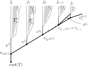
Figure 6. The thick black line represents $L\subset T$.

Possibly, $L$ contains only one vertex, namely $v_{1,d+1}$. This case immediately reduces to the case $d=1$ of a tree with two leaves. We do not discuss it anymore. If $d>1$, by collapsing the edge $e_{1}^{d+1}$ to its root and ignoring this point as a vertex one gets a new tree $\check{T}$ with $d$ leaves. By assumption, its ${\bf g}_{d-1}$-standard decoration fulfills all transversality requirements. The vertices $v_{1,d+1},v_{j_{{}_{1}},d+1},\ldots,v_{j_{r-1},d+1}$ are still there, with a different right label that we are going to neglect; as vertices of $\check{T}$ we denote them $\check{v}_{1},\check{v}_{j_{{}_{1}}},\ldots,\check{v}_{j_{{}_{r-1}}}$. The right branch issued from $\check{v}_{j_{{}_{r-1}}}$ in $\check{T}$ is a new branch whose label is $\check{e}^{j_{r}}$.

We have to understand how the graft of the last branch $e_{1}^{d+1}$ affects the multi-intersections at these vertices, that is, how we derive $I(v_{j_{{}_{\ell}},d+1})$ from $I(\check{v}_{j_{{}_{\ell}}})$ for every $\ell=0,\ldots,r-1$ (with the convention $j_{0}=1$). And what about $I(v_{j_{r},d+1})$—which does not exist in $\check{T}$—and the transversality to $\Sigma^{*}$? The other multi-intersections and stable manifolds coming from $\check{T}$ are kept without any change.

The manifolds $W^{s}(e^{j_{\ell}}),\ \ell=0,\ldots,r-1,$ including $W^{s}(\check{e}^{j_{r}})$, and their source maps $\sigma_{j_{{}_{\ell}}}$ valued in $M$ (noted $\sigma$ for short) are transversely defined by the decoration ${\bf g}_{d-1}$-standard, whatever the decoration of the last branch. This family of maps is transverse. Then the question is to find $g\in G$ so that this family remains transverse when adding one particular more map, namely the inclusion of $g(\Sigma)$.

First, we prove that $I(v_{j_{\ell},d+1})$ is transversely defined for a generic $g\in G$. We consider the diagram $\Delta(j_{\ell})$ whose limit (or iterated fiber product) $\lim\Delta(j_{\ell})$ is exactly the definition of the multi-intersection $I(\check{v}_{j_{\ell}})$.

Figure 7. Diagram $\Delta(j_{\ell})$

Note that the rightmost fiber product just produces $W^{s}(\check{e}^{j_{r}})$. Indeed, the graph of the flow and the stable manifold use the same vector field $X_{j_{r}}$. This is a trick that allows us to graft $W^{s}(e_{1}^{d+1})$ on $W^{s}(\check{e}^{j_{r}})$. The limit of $\Delta(j_{\ell})$ is equipped with a map $f_{\ell}:\lim\Delta(j_{\ell})\to M$ to the rightmost $M$ in the bottom line of the diagram. In this language, the requirement we want is the following.

(4.8) $$\quad\text{The inclusion }g\cdot W^{s}(e_{1}^{d+1},X^{+})\hookrightarrow M\text{ is transverse to }f_{\ell}.$$

By Proposition 3.2 this property is generic in $G$. The same holds if one requires the transversality to the family of all maps $f_{\ell},\ell=0,\ldots,r$. Of course, one has also to add all the requirements of item (2) in Definition 4.8 involving edges which do not meet the line $L$—all of them state transversality of family of source maps. The induction argument holds. $\Box$

Corollary 4.10.

For every admissible sequence ${\bf g}_{d}$, every Fukaya tree $T$ with $d+1$ leaves, and entries $(x_{1},...,x_{d+1})$, then the multi-intersection $I(T,\mathcal{D}_{{\bf g}_{d}},x_{1},...,x_{d+1})\subset M^{\times n(T)}$ is transversely defined. Its compactification has conical singularities. Moreover, this multi-intersection is mapped transversely to $\Sigma^{*}$ through the first projecton $p_{1}:M^{\times n(T)}\to M$. $\Box$

Proposition 4.11.

(Dimension formula) Given a generic Fukaya tree $T$ with $d$ leaves endowed with an admissible decoration and given entries $(x_{1},\ldots,x_{d})$, we have

(4.9) $$\quad\quad\dim I(T,x_{1},\ldots,x_{d})-n=\sum_{1\leq i\leq d}(\dim W^{s}(x_{i})-n)+d-2.$$

Proof. If we consider the Fukaya tree $T_{0}$ where all interior edges are collapsed, formula (4.9) where $d-2$ is erased (as there is no interior edge) reduces to the usual dimension formula for an intersection of $d$ submanifolds: it is additive up to the shift by the ambient dimension. Each time an interior edge is created, the dimension increases by 1 since some flow is needed which generates a stable set. $\Box$

4.12.

Multi-intersection as a chain.

In order to see the above multi-intersection $I(T,x_{1},\ldots,x_{d})$ as a chain in the Morse complex $C_{*}^{+}(f)$ whose degree is $\dim I(T)$, we have to define the coefficient $<I(T,x_{1},\ldots,x_{d}),x_{root}>$ for every test data $x_{root}\in critf\cup crit^{+}f_{\partial}$ of degree equal to $\dim I(T)$.

We recall the edge $e_{root}$ is decorated with the vector field $X^{+}$. Moreover, by Corollary 4.10 the projection $p_{1}:I(T)\to M$ to the first factor of $M^{\times n(T)}$ is transverse to $\Sigma^{*}$, and hence, to $W^{u}(x_{root},X^{+})$. By the choice of the degree of test data, the codimension of the unstable manifold $W^{u}(x_{root},X^{+})$ is equal to $\dim I(T,x_{1},...,x_{d})$. Transversality implies the intersection $I(T,x_{root}):=p_{1}^{-1}\left(W^{u}(x_{root},X^{+})\right)$ is 0-dimensional. Since its compact closure has conic singularities, this intersection is a finite set.

Being transversely defined in an oriented manifold, $I(T)$ is oriented, once an orientation has been chosen for every stable manifold of critical point. In the same time, the unstable manifolds are co-oriented. Therefore, each point in $I(T,x_{root})$ has a sign which allows us to define $<I(T),x_{root}>$ as the algebraic counting of elements in this finite set.

The map $<I(T,x_{1},\ldots,x_{d}),->$ from test data of the right degree to $\mathbb{Z}$ will be called the $T$-evaluation map. It depends on the admissible finite sequence ${\bf g}_{d-1}$ chosen in the group $G$.

5. Coherence

The $A_{\infty}$-structure that we want to reach requires to consider all Fukaya trees, generic or not, and to decorate them in a coherent way. We give the precise definition right below. The present section consists of mixing the skip property from Section 3 and the admissibility condition (Definition 4.8.) More precisely, the issue is to prove an analogue of Proposition 3.9 in the setting of trees with admissible decorations.

We first fix the setup for coherence. Given an infinite sequence ${\bf g}_{\infty}$ in the group $G=Dif\!f_{0}(M)$, a Fukaya tree $T$ and a subtree $T_{0}$ (Definition 4.2), then the ${\bf g}_{\infty}$-standard decoration of $T$ induces on $T_{0}$ a decoration $\mathcal{D}_{T}(T_{0})$ which, in general, differs from its own ${\bf g}_{\infty}$-standard decoration $\mathcal{D}_{{\bf g}_{\infty}}(T_{0})$; the labelling of this latter is consecutive and begins at $1$. Similarly, the quotient $T/T_{0}$ has also a decoration $\mathcal{D}(T/T_{0})$ inherited from $T$ which in general is not ${\bf g}_{\infty}$-standard; the shrinking of $T_{0}$ makes some gap in the decorating sequence.

Definition 5.1.

(provisional) 1) Two admissible decorations of $T$ are said to be isotopic if both lie in the same arcwise connected component of admissible decorations.

2) A sequence ${\bf g}_{d}$ is said to be coherent if it is admissible (that is, ${\bf g}_{d}\in\mathcal{A}_{d}$ in the sense of Definition 4.8) and, for every Fukaya tree $T$ with $d+1$ leaves and every subtree $T_{0}$, the decorations $\mathcal{D}_{T}(T_{0})$ and $\mathcal{D}(T/T_{0})$ inherited from $\mathcal{D}_{{\bf g}_{d}}(T)$ are both isotopic to their respective own ${\bf g}_{d}$-standard decoration.

An infinite sequence ${\bf g}_{\infty}$ is said to be coherent if its finite subsequences ${\bf g}_{d}$ are coherent for every $d$.

These two examples, $\mathcal{D}_{T}(T_{0})$ and $\mathcal{D}(T/T_{0})$, are examples of pruned trees in the sense of the next definition.

Definition 5.2.

A pruned tree is a tree with $k$ leaves and whose rightmost leaf is labelled $\ell>k$; that is, the labelling is not consecutive from $1$ to $k$. It is said to be a pruned tree with $\ell$ leaves.

From this point of view, if $T_{0}$ is a Fukaya subtree of $T$ with no leaf labelled $1$, then $\mathcal{D}_{T}(T_{0})$ looks as a particular case where the pruning reads $[1,r)$. In contrast, if 1 is the label of the leftmost leaf of $T_{0}$ the pruning is entirely made on the right of $T$ and has no effect on the decoration of $T_{0}$; it will be said to be a useless pruning. The notion of admissibility extends to the pruned trees.

Definition 5.3.

A sequence ${\bf g}_{d}$ of diffeomorphisms of $M$ isotopic to $Id_{M}$ is said to be coherent if the following two conditions are fulfilled:

1. for every tree with $d+1$ leaves, pruned or not, the (induced) ${\bf g}_{d}$-standard decoration is admissible;

2. if such a tree is pruned, its induced decoration is isotopic to its own ${\bf g}_{d}$-standard decoration among the admissible decorations.

An infinite sequence ${\bf g}_{\infty}$ is said to be coherent if its finite subsequences ${\bf g}_{d}$, consecutive from $1$, are coherent for every $d$.

Proposition 5.4.

There exists a coherent infinite sequence of diffeomorphisms of $M$ whose restriction to the preferred neighborhood $V(\Sigma)$ of $\Sigma$ in $M$ is made of quasi translations.

Proof. This will be proved by an induction on $d$ starting at $d=1$. It is somehow a combination of Proposition 3.13 about the skip property and Proposition 4.9 about admissibility. For $d=1$, there is no pruning; so, the statement reduces to transverse intersection.

As for Proposition 3.13 we use quasi translation flows which are provided to us by Proposition 3.8. Assume we have a sequence ${\bf g}_{d-1}$ whose elements are quasi translations $g_{1}=v_{0}^{t_{1}},\ldots,g_{d-1}=v_{d-2}^{(t_{d-1}-t_{d-2})}$ which form a coherent sequence of length $d-1$. Since the transversality requirements are open conditions some time $t_{d}>t_{d-1}$ is available.

But increasing by $1$ the number of leaves imposes to satisfy new transversality requirements which make necessary to approximate the flow $v_{d-2}$ by a suitable $v_{d-1}$ (compare to the proof of item (2) from Proposition 3.8.) The new requirements in question are essentially those resulting from diagrams like $\Delta(j_{\ell})$ (see Figure 7). Here, it should be noted that the family of quasi translations is reach enough for providing us with finite dimensional families which are submersive onto the preferred neighborhood $V(\Sigma)$. Therefore, the transversality theorem to a singular map is available among quasi translations.

At this point, we have a new proof of Proposition 3.8). But working with flows provides us with the so-called transversality-to-path (item (3) from Proposition 3.8.) Therefore we get the skip property in the context of Fukaya tree admissibility, which is the same as coherence for pruned trees with gap of length one. As in Corollary 3.12, coherence for general prunings follows. $\Box$

6. Transition

Proving $A_{\infty}$-relations in Section 8 requires to analyse the transition phenomenon from $I(T^{\prime})$ to $I(T^{\prime\prime})$, where $T^{\prime}$ and $T^{\prime\prime}$ are two “generic” Fukaya trees with $d$ leaves on each side of a “codimension-one stratum” in the space $\mathcal{T}_{d}$ of Fukaya trees with $d$ leaves (cf. just after Definition 4.1).

6.1.

Setting of transition. We consider two Fukaya trees $T^{\prime}$ and $T^{\prime\prime}$ which differ only in the star of $v$ (see Figure 8). The intermediate Fukaya tree $T$ has exactly one vertex $v$ whose valency is 4. Up to isotopy, $T^{\prime}$ and $T^{\prime\prime}$ are the only two possible deformations from $T$ to a generic tree. The edge $e^{\prime}$ (resp. $e^{\prime\prime}$) is collapsed in $T^{\prime}\to T$ (resp. $T^{\prime\prime}\to T$). The counting of interior edges gives $n(T^{\prime})=n(T^{\prime\prime})=n(T)+1$.

Since Proposition 5.4 applies to trees, generic or not, if ${\bf g}_{\infty}=g_{1},g_{2},\ldots$ is an infinite coherent sequence in the group $G$ then the sequence of vector fields

$$X^{+},g_{1*}X^{+},\dots,g_{(d-1)*}X^{+}$$

is a sequence of coherent ${\bf g}_{d-1}$-standard decorations common to $T^{\prime}$, $T$ and $T^{\prime\prime}$ where ${\bf g}_{d-1}$ is the beginning subsequence of length $d$ in ${\bf g}_{\infty}$. In the next proposition $I(T^{\prime}),I(T),I(T^{\prime\prime})$ will denote the respective multi-intersections at the vertex $v^{root}$, right above their common root: the above decorations are implicit and the entries are arbitrary critical points in $critf\cup crit^{+}f_{\partial}$ with possible repetition.

Figure 8.

Proposition 6.2.

In this setting, the multi-intersection $I(T)$ has a natural smooth embedding $j^{\prime}:I(T)\to I(T^{\prime})$, respectively $j^{\prime\prime}:I(T)\to I(T^{\prime\prime})$), as a boundary stratum. These embeddings extend to the closure $cl\bigl{(}I(T)\bigr{)}$ in a way compatible with the stratifications. Then, $I(T^{\prime})\mathop{\cup}\limits_{I(T)}I(T^{\prime\prime})$ is a (piecewise smooth) manifold which is equipped with a natural stratified compactification.

Note this amalgamation is not contained in $M^{\times(n(T)+1)}$. It can only be piecewise immersed into that, with a fold along $I(T)$.

Proof. It is sufficient to focus on the subtrees $T(v_{0})$, $T^{\prime}(v_{0})$ and $T^{\prime\prime}(v_{0})$ rooted at $v_{0}$ (Figure 8). Since $T^{\prime}$ and $T^{\prime\prime}$ play the same role with respect to $T$, we look only at $T(v_{0})$ and $T^{\prime}(v_{0})$.

On the one hand, the multi-intersection $I(v,T)$ is contained in $M^{\times n(v,T)}$ where $n(v,T)-1$ is equal to the number of interior edges of $T$ lying above $v$. We have

(6.1) $$I(v,T)=\left(W^{s}(e_{1})\mathop{\times}\limits_{M}W^{s}(e_{2})\right)\mathop{\times}\limits_{M}W^{s}(e_{3})\,,$$

where the fiber product is associative. On the other hand, $I(v,T^{\prime})$ is contained in $M^{\times n(v,T^{\prime})}$ and the graph $G_{e^{\prime}}$ of the semi-flow associated with the decoration of $e^{\prime}$ is contained in the product of the first two factors of $M^{\times n(v,T^{\prime})}$. Thus, there is a—partially—diagonal map

(6.2) $$\left\{\begin{array}[]{ccc}\quad\quad J:M^{\times n(v,T)}&\to&M^{\times n(v,T^{\prime})}\\ (x,y,z,\ldots)&\mapsto&(x,x,y,z,\ldots)\end{array}\right.$$

Observe that $I(v^{\prime},T^{\prime})$ is canonically isomorphic to $W^{s}(e_{1})\mathop{\times}\limits_{M}W^{s}(e_{2})$ the amalgamation being made through the source map $\sigma$ of the respective factors—actually the projection to the first factor. Therefore, we have:

(6.3) $$I(v,T)=J^{-1}\left(\Bigl{(}G_{e^{\prime}}\mathop{\times}\limits_{M}I(v^{\prime},T^{\prime})\Bigr{)}\mathop{\times}\limits_{M}W^{s}(e_{3})\right)\,.$$

As a consequence, $J$ induces the desired embedding $j^{\prime}$, which is a boundary because the diagonal is a boundary of $G_{e^{\prime}}$. $\Box$

7. Orientations

The matter of orientation is a question of Linear Algebra. Some conventions have to be chosen.

7.1.

Orientation, co-orientation and boundary.

1) Let $E$ be a vector subspace of an oriented vector space $V$. Let $\nu(E,V)$ be a complement to $E$ in $V$. Then, the orientation and the co-oriention of $E$ will be related as follows:

(7.1) $$or\bigl{(}\nu(E,V)\bigr{)}\wedge or(E)=or(V).$$

2) Let $E$ be a half-space with boundary $B$. Let $\varepsilon$ be a vector in $\nu(B,E)$ pointing outwards, where $\nu(B,E)$ is a complement to $B$ in $span(E)$. Then, the orientations of $B$ and $E$ will be related as follows:

(7.2) $$\varepsilon\wedge or(B)=or(E).$$

When $E$ is oriented, this orientation of $B$ is called the boundary orientation; it is denoted by $or_{\partial}(B,E)$; one also says that $B$ is the oriented boundary of $E$. Notice that, when $E\subset V$, the choices 1) and 2) are compatible if we choose $\nu(B,V)=\nu(E,V)\oplus\varepsilon\mathbb{R}$.

7.2.

Orientation and fiber product. Let $E_{1},E_{2},V$ be three oriented vector spaces and, for $i=1,2$, let $f_{i}:E_{i}\to V$ be a linear map. Assume that $f_{1}\times f_{2}:E_{1}\times E_{2}\to V\times V$ is transverse to the diagonal $\Delta$. Then the fiber product $E_{12}:=E_{1}\mathop{\times}\limits_{V}E_{2}$ is well-defined as the inverse image of $\Delta$ by $f_{1}\times f_{2}$.

The first factor of $V\times V$ is seen as a complement to $\Delta$ in $V\times V$. So, the orientation of $V$ defines a co-orientation of the diagonal. Transversality to $\Delta$ yields a canonical isomorphism $\nu(E_{12},E_{1}\times E_{2})\cong\nu(\Delta,V\times V)$. Thus, $E_{12}$ is co-oriented in $E_{1}\times E_{2}$. Eventually, it is oriented according to (7.1).

Proposition 7.3.

In the case when a fiber product with three factors is defined, the orientation is associative, that is: $\left(E_{1}\mathop{\times}\limits_{V}E_{2}\right)\mathop{\times}\limits_{V}E_{3}$ and $E_{1}\mathop{\times}\limits_{V}\left(E_{2}\mathop{\times}\limits_{V}E_{3}\right)$ have the same orientation.

Proof. It is sufficient to look at the small diagonal $\delta_{3}$ in $V\times V\times V$. In the first case it is seen as the diagonal of $\Delta\times V$ and in the second case it is seen as the diagonal $V\times\Delta$. In both cases, its co-orientation is induced by the orientation of the first $V\times V$. $\Box$

In the setting of subsection 7.2, we have the following formulas.

Proposition 7.4.

1) Let $E_{1}$ be an oriented linear half-space with oriented boundary $B_{1}$ and let $E_{2}$ be an oriented vector space. Assume that the restriction $f_{1}\times f_{2}|(B_{1}\times E_{2})$ is transverse to $\Delta$. Then, the fiber product $B_{12}:=B_{1}\mathop{\times}\limits_{V}E_{2}$ is the boundary of $E_{12}$ and its orientation coincides with the boundary orientation, that is:

(7.3) $$or_{\partial}\left(B_{12},E_{12}\right)=or\left(B_{1}\mathop{\times}\limits_{V}E_{2}\right)\,.$$

2) Let $E_{2}$ be now an oriented linear half-space with an oriented boundary $B_{2}$ and let $E_{1}$ be an oriented vector space. Assume that the restriction $f_{1}\times f_{2}|(E_{1}\times B_{2})$ is transverse to $\Delta$. Then, the fiber product $B_{12}:=E_{1}\mathop{\times}\limits_{V}B_{2}$ is the boundary of $E_{12}$. The orientations are related as follows:

(7.4) $$or_{\partial}\left(B_{12},E_{12}\right)=(-1)^{\dim E_{1}}or\left(E_{1}\mathop{\times}\limits_{V}B_{2}\right)\,.$$

Proof. In both cases the co-orientation of $B_{12}$ in the boundary $\partial\left(E_{1}\times E_{2}\right)$ is induced by the co-orientation of the diagonal $\Delta$. So, the only difference depends on the boundary orientation of $\partial\left(E_{1}\times E_{2}\right)$. In the first case, the boundary orientation is the product orientation $or_{\partial}(B_{1},E_{1})\wedge or(E_{2})$. In the second case, we have:

$$or_{\partial}\left(\partial(E_{1}\times E_{2}),E_{1}\times E_{2}\right)=(-1)^{\dim E_{1}}or(E_{1})\wedge or_{\partial}(B_{2},E_{2})\,.$$

$\Box$

Of course, all of that was previously said in the linear case applies word to word in the non-linear case to fiber products of manifolds with boundary when they are defined, that is, under some transversality assumptions. The intersection of two transverse submanifolds is a particular case of the previous discussion.

Orientation and graph of a semi-flow. Let $e$ be an edge (interior or not) in a decorated Fukaya tree $(T,\mathcal{D})$ and let $X_{e}$ be the gradient decorating $e$. Let $G_{e}$ be the graph of its positive semi-flow $\bar{X}_{e}$. The source map $\sigma_{e}$ makes $G_{e}$ a $[0,+\infty)$-bundle over $M$. By convention, $G_{e}$ will be oriented like $or([0,\infty))\wedge or(M)$. Recall also the target map $\tau_{e}:G_{e}\to M,\ (t,x)\mapsto\bar{X}_{e}^{t}(x)$.

Proposition 7.5.

Let $z\in critf\cup crit^{+}f_{\partial}$ and let $H$ be the codimension-one stratum in the closure of $G_{e}\subset M\times M$ made of orbits that are broken at $z$. Denote by $\dot{W}^{s}(z)$ the stable manifold punctured at $z$; and similarly for the unstable manifold $\dot{W}^{u}(z)$. Then we have

(7.5) $$H=\dot{W}^{s}(z)\times\dot{W}^{u}(z)$$

as oriented manifolds where $H$ is oriented as a boundary component of $G_{e}$. Moreover, the right handside of (7.5) is a sub-product of $M\times M$.

Proof. First, recall that $W^{u}(z)$ is oriented arbitrarily; it is also co-oriented so that $co$-$or(W^{u}(z))\wedge or(W^{u}(z))=or(M)$. By convention the stable manifold is oriented by the co-orientation of the unstable manifold. Thus, the right hand side of (7.5) has the orientation of $M$.

Now, take a pair $(x,y)\in\dot{W}^{s}(z)\times\dot{W}^{u}(z)$ and a small $\varepsilon>0$. Set $a=x+\varepsilon\vec{zy}$ in the affine structure of the Morse model about $z$. The orbit of $a$ intersects the affine line $y+\mathbb{R}\vec{zx}$ in exactly one point $a^{\prime}$ at some time $t^{\prime}$; we have $\bar{X}^{t^{\prime}}_{e}(a)=a^{\prime}$. So, for some small enough $\delta$ and $0<\varepsilon<\delta$, we have a collar map

$$\begin{array}[]{ccc}C:(0,\delta)\times\dot{W}^{s}(z)\times\dot{W}^{u}(z)&\longrightarrow&G_{e}\\ (\varepsilon,x,y)&\mapsto&(a,a^{\prime})\end{array}$$

which extends to a diffeomorphism $\{0\}\times\dot{W}^{s}(z)\times\dot{W}^{u}(z)\cong H$. By a computation in the Morse model, it is seen that, fixing $\varepsilon$, the map $\tau_{e}\circ C_{\varepsilon}:(x,y)\mapsto a^{\prime}$ is orientation preserving. Moreover, making $\varepsilon$ decrease (which is the outgoing direction along the boundary) makes $t^{\prime}$ increase. Altogether, we have the desired isomorphism of orientations. $\Box$

Orientation and multi-intersection.

Let $T$ be a generic tree with $d$ leaves, an admissible decoration $\mathcal{D}$ and entries $x_{1},...,x_{d}$. Here we consider the case where $e$ is the trunk of $T$ (see right after Definition 4.1). Suppose $z\in crit_{*}f\cup crit_{*-1}^{+}f_{\partial}$ has a degree (that is its value of $*=\dim W^{s}(z)$) which is equal to $\dim I(T,\mathcal{D},x_{1},...,x_{d})$. Let $\sigma_{e}:G_{e}\to M$ be the source map.

Then $z$ determines a codimension-one stratum $H$ (possibly empty), made of orbits broken at $z$, in the closure of $W^{s}(e)\subset M^{\times n(e)}$. This $H$ is mapped by $\sigma_{e}$ transversely to the unstable manifold $W^{u}(z)$ since the decoration is admissible. By the dimension assumption, the intersection $\sigma_{e}^{-1}(W^{u}(z))\cap H$ is made of a finitely many signed points.

Definition 7.6.

The sum $\mu(z)$ of the above signs is named the (algebraic) multiplicity of $H$ as a boundary component of $W^{s}(e)$. It is also the coefficient of $z$ in the chain represented by $I(T,x_{1},...,x_{d})$ (an admissible decoration being implicit—see subsection 4.12).

Finally, let $T_{0}$ be a strict sub-tree of $T$ with $k$ leaves, let $e$ be the trunk of $T_{0}$, an interior edge of $T$. This time, $z$ is assumed to generate a codimension-one stratum $H$ in the closure of $W^{s}(e,x_{j+1},...,x_{j+k})$ where $j$ is the label of the leaf which lies just to the left of the leaves of $T_{0}$.

Proposition 7.7.

Consider the above setting. Then $H$ contributes to a boundary stratum in the closure of the multi-intersection $I(T)$ with the multiplicity $(-1)^{\varepsilon_{j}}\mu(z)$ where

(7.6) $$\varepsilon_{j}=n+j-1+\sum_{i=1}^{j}(\dim W^{s}(x_{i})-n)\,.$$

Note the difference between Definition 7.6 and Proposition 7.7: the breaking of orbits takes place just below (resp. above) the considered multi-intersection in the first (resp. second) case. In the latter, $H$ contributes to the differential $\partial^{+}$ of the chain that $I(T,x_{1},...,x_{d})$ represents in the complex $C^{+}_{*}$.

Proof. It consists of a generalization to fiber products of the sign given in the case of a product by Proposition 7.4. A codimension-one stratum remains so through fiber products of transverse mappings and transverse intersections.

Note that the sign we are interested in is invariant by sliding the edges (see the transition move on Figure 8) as long as the edges to the left of the leftmost complete path (that is, from the root to a leaf) which contains $e$ are not involved.

After a well-chosen sequence of such transitions, $T$ has the following form: $T(v_{1})=T_{\alpha}\mathop{\vee}\limits_{v_{1}}T_{\beta}$. Here, $v_{1}$ is the first interior vertex above the root of $T$ and $T(v_{1})$ stands for the union of edges above $v_{1}$; the $\vee$ means the bouquet; $T_{\alpha}$ is a tree with $j$ leaves and the edge root of $T_{\beta}$ is $e$. In that case, the multi-intersection becomes a usual—not iterated—fiber product and its left factor has a dimension equal to $\dim I(T_{\alpha},x_{1},...,x_{j})+1$. The dimension formula (4.9) and Proposition 7.4 yield the desired sign. $\Box$

Orientation and gluing. Here we go back to the setting of subsection 6.1. We will prove the following statement:

Proposition 7.8.

The two multi-intersections $I(T^{\prime})$ and $I(T^{\prime\prime})$, equipped with their natural orientations, give $I(T)$ two opposite boundary orientations. In other words, the amalgamation $I(T^{\prime})\mathop{\cup}\limits_{I(T)}I(T^{\prime\prime})$ is made in the category of oriented manifolds.

Proof. First we observe that the decoration has no effect on orientation matter. So, without loss of generality, we may assume $X_{e^{\prime}}=X_{e^{\prime\prime}}$ (notation of Figure 8). We are now going to use formulas (6.1) and (6.2) from the proof of Proposition 6.2. Each factors in the iterated fiber product diagram (6.1) is contained in some $M^{\times q}$ and the maps in the diagram of fiber product are induced by the first coordinate in each factor. In coordinates, a point $a\in I(v,T)$ reads:

(7.7) $$\begin{array}[]{lc}&a=\left\{(x_{1},\ldots,x_{k})(y_{1},\ldots,y_{\ell})(z_{1},\ldots,z_{m})\right\}\\ &x_{1}=y_{1}=z_{1}\end{array}$$

where each coordinate $x_{i},y_{i}$ or $z_{i}$ denotes a point in $M$. Any point $a^{\prime}$ in $I(v,T^{\prime})$ reads

(7.8) $$\begin{array}[]{lc}&a^{\prime}=\left\{(s^{\prime},t^{\prime})(x_{1},\ldots,x_{k})(y_{1},\ldots,y_{\ell})(z_{1},\ldots,z_{m})\right\}\\ &t^{\prime}=x_{1}=y_{1},\ s^{\prime}=z_{1},\end{array}$$

where the new coordinates $(s^{\prime},t^{\prime})$ are those of $G_{e^{\prime}}$, source and target. Similarly, any point $a^{\prime\prime}$ in $I(v,T^{\prime\prime})$ reads:

(7.9) $$\begin{array}[]{lc}&a^{\prime\prime}=\left\{(x_{1},\ldots,x_{k})(s^{\prime\prime},t^{\prime\prime})(y_{1},\ldots,y_{\ell})(z_{1},\ldots,z_{m})\right\}\\ &s^{\prime\prime}=x_{1},\ t^{\prime\prime}=y_{1}=z_{1},\end{array}$$

where the coordinates $(s^{\prime\prime},t^{\prime\prime})$ are those of $G_{e^{\prime}}$, source and target. When comparing formulas (7.8) and (7.9) at a point of $I(v,T)$, we get $s^{\prime\prime}=t^{\prime},\ t^{\prime\prime}=s^{\prime}$. This corresponds to reversing the time of the flow of $X_{e^{\prime}}=X_{e^{\prime\prime}}$. Then, the time is the only variable whose orientation is changed. This is the reason why the orientation of $I(T)$ changes depending on $I(T)$ is seen as a boundary of $I(T^{\prime})$ or $I(T^{\prime\prime})$. The change of the place of the couple (source, target) has no effect on the orientation since it is an equidimensional couple. $\Box$

8. $A_{\infty}$-structure

In this section, we exhibit how one can construct an $A_{\infty}$-structure on the Morse complex $A=C_{*}(f,X^{+})$ whose first operation $m_{1}$ coincide with the differential $\partial^{+}$. The grading is now defined by setting $|x|:=n-\dim W^{s}(x)$ for every critical point $x\in critf\cup crit^{+}f_{\partial}$. Note this grading is cohomological, that is, the degree of the differential $m_{1}=\partial^{+}$ is $+1$.

One fixes a coherent sequence ${\bf g}_{\infty}$ in the group $G$. Every Fukaya tree $T$ is endowed with the ${\bf g}_{\infty}$-standard decoration $\mathcal{D}(T)$. So, for any tree $T$ with $d\geq 2$ leaves and any sequence of $(d+1)$ critical points $x_{1},\ldots x_{d},x_{d+1}$ (with possible repetition) we have the multi-intersection $I(T,x_{1},\ldots x_{d};x_{d+1})$ defined by the following fiber product (compare to the $T$-evaluation map defined at the end of subsection 4.12):

(8.1) $$I(T,x_{1},\dots,x_{d};x_{d+1}):=\lim\left(I(v_{root}^{1})\mathop{\longrightarrow}\limits^{{}^{p_{root}}}M\mathop{\longleftarrow}\limits^{j}W^{u}(x_{d+1},X^{+})\right)\$$

We recall that $v^{1}_{root}$ is the terminal vertex of the edge originating at the root and the associated generalized intersection is defined inductively in Section 4. Since $\mathcal{D}(T)$ is admissible, this set is a manifold. Using the dimension formula of Proposition 4.11, we conclude that its dimension is

(8.2) $$\dim I(T,x_{1},\dots,x_{d};x_{d+1})=d-2+|x_{d+1}|-\sum_{i=1}^{k}|x_{i}|.$$

Therefore the dimension of $I(T,x_{1},\cdots x_{d};x_{d+1})$ is zero if and only if

$$|x_{d+1}|=\sum_{i=1}^{k}|x_{i}|+2-d$$

In what follows, we denote by $\mathcal{T}^{0}$ (resp. $\mathcal{T}^{0}_{d}$) the set of generic Fukaya trees (resp. with $d$ leaves). For $d\geq 2$, we define the linear maps $m_{d}:A^{\otimes d}\to A$ by

(8.3) $$\left\{\begin{split}&m_{d}(x_{1},\dots,x_{d}):=\\ &(-1)^{\sum_{s=1}^{d}(d-s)|x_{s}|}\sum_{T\in\mathcal{T}^{0}_{d}}\left[\sum_{|y|=2-d+\sum|x_{i}|}\#I(T,x_{1},\dots,x_{d};y)y\right].\end{split}\right.$$

One should think of $I(T,x_{1},\dots,x_{d};y)$ as an oriented zero-dimensional manifold and $\#I(T,x_{1},\dots,x_{d};y)$ is the algebraic number of signed points in this manifold. It is clear from the definition that the degree of $m_{d}$ is $2-d$.

8.1.

Geometric definition of the first operation. So far, we have not considered trees with just one leaf. Nevertheless, for $x\in critf\cup crit^{+}f_{\partial}$, one can define $m_{1}(x)$ geometrically in the following way. From the compactification of $W^{s}(x,X^{+})$ one extracts the frontier $F^{s}(x)$ which is the complement of $W^{s}(x,X^{+})$ in its closure. As $X^{+}$ is Morse-Smale, $F^{s}(x)$ is transverse to $W^{u}(y,X^{+})$ for every $y\in critf\cup crit^{+}f_{\partial}$. When $|y|=|x|+1$, one defines the 0-dimensional intersection manifold $I(x;y):=F^{s}(x)\cap W^{u}(y,X^{+})$. As it is oriented, it is made of a finite set of signed points. Then one defines

(8.4) $$m_{1}(x)=\sum_{|y|=|x|+1}\#I(x;y)y\,.$$

Theorem 8.2.

$(A,m_{1},m_{2},\dots)$ is an $A_{\infty}$-algebra.

Proof.  The $A_{\infty}$-relations read for every $d>0$:

(8.5) $$\sum_{j,k,l}(-1)^{j+k\ell}m_{j+1+\ell}(1^{\otimes j}\otimes m_{k}\otimes 1^{\otimes l})=0$$

where the sum is taken over all non-negative integers $j,k,l$ such that $j+k+l=d$.

When putting entries $(x_{1},\dots,x_{d})$, new signs appear according to Koszul’s rule:

(8.6) $$\begin{split}&(1^{\otimes j}\otimes m_{k})(x_{1},\ldots,x_{j},x_{j+1},\dots,x_{j+k})=\\ &(-1)^{(|x_{1}|+\dots+|x_{j}|)|m_{k}|}\bigl{(}x_{1},\ldots,x_{j},m_{k}(x_{j+1},\dots,x_{j+k})\bigr{)},\end{split}$$

and Identity (8.5) becomes:

(8.7) $$\sum_{j+k+l=d}(-1)^{\varepsilon}m_{j+1+l}(x_{1},\dots,x_{j},m_{k}(x_{j+1},\dots,x_{j+k}),x_{j+k+1},\dots,x_{d})=0,$$

where $\varepsilon=j+kl+(2-k)(\sum_{i=1}^{j}|x_{i}|)$.

By the very definition of the $m_{k}$’s, the above $A_{\infty}$-relations are equivalent to the following identities

(8.8) $$\sum_{j,k,T_{\alpha},T_{\beta}}\sum_{y}(-1)^{\varepsilon^{\prime}}\#I(T_{\alpha},x_{j+1},\dots,x_{j+k};y)\,\#I(T_{\beta},x_{1},\dots,x_{j},y,x_{j+k+1},\dots x_{d};z)=0$$

for all $d\geq 1$ and all sequence $(x_{1},\dots,x_{d},y,z)$ of critical points with $|y|=2-k+\sum_{i=j+1}^{j+k}|x_{i}|$, $|z|=3-d+\sum_{i=1}^{d}|x_{i}|$ and $\varepsilon^{\prime}=|x_{1}|+\cdots|x_{j}|-j$. In this sum, $T_{\alpha}$ is a generic tree with $k$ leaves and $T_{\beta}$ is a generic tree with $d-k+1$ leaves. By (8.2), the manifold $I(T_{\beta},x_{1},\dots,x_{j},y,x_{j+k+1},\dots x_{d};z)$ is 0-dimensional.

Note that, from $|z|=3-d+\sum_{i=1}^{d}|x_{i}|$, it follows that for every generic tree $T$ the multi-intersection $I(T,x_{1},\dots,x_{j+k+l};z)$ is one-dimensional.

The proof of (8.8) will follow from analysing the frontier of this oriented manifold in its compactification (we know from Appendix A that the multi-intersections are compact manifolds with $C^{1}$ conic singularities.)

We fix a generic tree $T$ with $d$ leaves and consider the compact 1-dimensional submanifold with conic singularities $cl(I(T,x_{1},\dots,x_{d};z))\subset M^{\times(d-1)}$. By blowing up the singular points, such a manifold can be thought of as a manifold with boundary where some boundary points are identified. Such a point $P$ is equipped with a sign which is the sum of the boundary-orientation signs of the inverse images of $P$ in the above blowing up, which is itself oriented. Therefore, we have:

(8.9) $$\sum_{P\,\in\,\partial\bigl{(}cl(I(T,x_{1},\dots,x_{d};z))\bigr{)}}sign(P)=0$$

By iterating Proposition 7.5, the boundary components of the closure $cl(I(T,x_{1},\dots,x_{d};z)\bigr{)}$ are divided into three types:

Type A: The boundary components coming from the broken orbits in the compactification of the generalized stable manifold $W^{s}(e,X_{e})$. Here, $e$ is an interior edge in the tree $T$ and $X_{e}$ is its decoration. Such a codimension-one stratum involves some critical point $y$ and its invariant manifolds with respect to $X_{e}$. Therefore, it is of the form

$$I(T_{\alpha},x_{j+1},\dots,x_{j+k};y)\times I(T_{\beta},x_{1},\dots,x_{j},y,x_{j+k+1},\dots x_{d};z),\ 0\leq k\leq d.$$

The first (resp. second) factor in this product comes from the unstable (resp. stable) manifold of $y$. The tree $T$ is equal to the connected sum

$$T=T_{\alpha}\#_{j+1}T_{\beta}$$

where the root of $T_{\alpha}$ is glued to the $(j+1)$-th leaf of $T_{\beta}$.

Type B: The boundary components of the form $I(T/e,x_{1},\dots,x_{d};z)$ where $e$ is an interior edge of $T$ and $T/e$ denotes the tree obtained from $T$ by collapsing $e$ to a point. They are induced by the diagonal of $M\times M$ except over the zeroes of the vector field $X_{e}$ which decorates $e$.

Type C: The boundary components which are induced by $\partial M$. In general, a stable manifolds has orbits coming from $\partial M$. Actually, the type-C components are empty in the considered multi-intersection $I(T,x_{1},\dots,x_{d};z)$. Indeed, by construction, the unstable manifold $W^{u}(z,X^{+})$ lies in the interior of $M$ except very near $z$ if $z\in crit^{+}f_{\partial}$. Thus, the multi-intersection $I(T,x_{1},\dots,x_{d};z)$, that is the evaluation $<I(T,x_{1},\dots,x_{d}),z>$, has no type-C boundary components.

Therefore the identity (8.9) splits into the sum of two terms

(8.10) $$S_{A}+S_{B}=0$$

where $S_{A}$ (resp. $S_{B}$) is the contribution of the type-A (resp. type-B) components. Note that $S_{A}$ is exactly the left handside of Equation (8.8) since $T$, $j$ and $k$ determine $T_{\alpha}$ and $T_{\beta}$. Therefore, we are reduced to prove the nullity of $S_{B}$.

By Proposition 6.2, a type $B$ boundary component $I({T/e},x_{1},\cdots,x_{d};z)$ appears as a boundary component of exactly one another one-dimensional intersection submanifold $I({T^{\prime}},x_{1},\cdots,x_{d};z)$ where $T^{\prime}$ is the unique generic tree, distinct from $T$, obtained from $T/e$ by an expansion at its unique degree-$4$ vertex (see Figure 8). Moreover, by Proposition 7.8, the induced orientations are opposite. Therefore, in the sum $S_{B}$ these two terms cancel each other out.

Checking of the signs. We apply Proposition 7.7 which gives us the following sum of chains of geometric nature (without evaluating):

(8.11) $$\partial^{+}I(T,x_{1},\dots,x_{d})=\sum_{j,k,y}(-1)^{\varepsilon_{j}}\#I(T_{\alpha},x_{j+1},\dots,x_{j+k};y)\,\partial^{+}I(T_{\beta},x_{1},\dots,y,x_{j+k+1},\dots,x_{d}).$$

Here, $j$ varies from 1 to $d-1$; $k$ from 1 to $d-j$; $y$ is a critical point such that $|y|=2-k+\sum|x_{i}|$ and the geometric sign is the one given by formula 7.6, that is,

$$\varepsilon_{j}=n+j-1+\sum_{i=1}^{j}(\dim W^{s}(x_{i})-n)=n+j-1-\sum_{i=1}^{j}|x_{j}|.$$

$\Box$

9. Morse concordance and homotopy of $A_{d}$ -structures

We have seen that the operations $m_{1},m_{2},\dots$ which define an $A_{\infty}$-structure on the complex $A:=C_{*}(f,X^{+})$ are determined by the choice of a family of coherent decorations for every Fukaya tree $T$. Recall that a decoration of an edge $e$ is a vector field $X_{e}$ approximating $X^{+}$. In particular, it lies in the same connected component of Morse-Smale vector fields.

Assume we have two coherent sequences ${\bf g}_{\infty}$ and ${\bf g}^{\prime}_{\infty}$ in the group $G=Di\!f\!f_{0}(M)$ and their associated standard decorations $\{\mathcal{D}(T)\}_{T}$ and $\{\mathcal{D}^{\prime}(T)\}_{T}$, decorating all Fukaya trees. In general, these two families give rise to two distinct $A_{\infty}$-structures $(m_{1},m_{2},\dots)$ and $(m^{\prime}_{1},m^{\prime}_{2},\dots)$. We are going to show that these two structures can be linked by a homotopy thanks to multi-intersections over the product manifold $\hat{M}:=M\times[0,1]$ which is a manifold with boundary and corners. Note that the complex $C_{*}(f,X^{+})$ is kept unchanged; in particular, $m_{1}=m^{\prime}_{1}$. A multi-intersection $\hat{I}(T)$ over $\hat{M}$ associated with a decoration $\hat{\mathcal{D}}(T)$ will be thought of as a cobordism from its trace over $M\times\{0\}$ to its trace over $M\times\{1\}$. Such a family of cobordisms will be called a geometric homotopy. The expression Morse concordance from the section title emphasizes the fact that the underlying manifold is a product $M\times[0,1]$ equipped with a function without critical points in its interior.

Here, we are inspired by Conley’s continuation map [5] that we have extended to the $A_{\infty}$-case. The case of the Morse complex is discussed in [23] and [11] as a prelude to the (infinite dimensional) case of Floer homology. In fact, Andreas Floer [7] had first evoked the idea for the infinite dimensional Morse Theory. The invariance of the Morse homology was proved earlier using other methods.

9.1.

Construction of a Morse concordance.

For simplicity, we first restrict to the case where $\partial M$ is empty. Then, $\hat{M}:=M\times[0,1]$ is a manifold with boundary. The general case will be sketched in Remark 9.4. When $\partial M=\emptyset$, we consider a Morse-Smale pseudo-gradient $X$ adapted to the Morse function $f$.

We first build a Morse function $\hat{f}$ on $\hat{M}$ with no critical points in the interior of $\hat{M}$ whose restriction to $M_{i}:=M\times\{i\}$, $i=0,1$, reads $\hat{f}|_{M_{i}}=f+c_{i}$ where $c_{i}$ is some constant. More precisely, one requires the critical points of $\hat{f}|_{M_{0}}$ to be of type $+$ and those of $\hat{f}|_{M_{1}}$ to be of type $-$. The pseudo-gradient vector fields adapted to $\hat{f}$ are required to be tangent to the boundary. This needs a slight modification with respect to the Morse theory we have considered so far.

Let $h:\mathbb{R}\to\mathbb{R}$ be the Morse function defined by $h(t)=(2t-1)^{3}-3(2t-1)$; its critical points are $t=0,1$. For $(x,t)\in\hat{M}$, set $\hat{f}(x,t)=f(x)+h(t)$. If $a$ is a critical point in $M_{0}$ (resp. in $M_{1}$), we have:

(9.1) $$Ind(\hat{f},a)=Ind(f,a)+1\quad(\text{resp. }=Ind(f,a))\,.$$

If $\hat{X}$ is a pseudo-gradient on $\hat{M}$ adapted to $\hat{f}$ and tangent to $M_{0}\cup M_{1}$, depending on $a\in M_{0}$ (resp. $a\in M_{1}$), the stable manifold $W^{s}(a,\hat{X})$ (resp. the unstable manifold $W^{u}(a,\hat{X})$) meets the interior of $\hat{M}$; on the contrary, the unstable (resp. stable) manifold lies entirely in $M_{0}$ (resp. in $M_{1}$).

The critical points of $\hat{f}$ in $M_{0}$ will serve as entries; those lying in $M_{1}$ will be used as test data. Consider now an edge $e\subset T$ and its two decorations $X_{e}\in\mathcal{D}(T)$ and $X^{\prime}_{e}\in\mathcal{D}^{\prime}(T)$. Since $X_{e}$ and $X^{\prime}_{e}$ are approximations of the same Morse-Smale vector field $X^{+}$ on $M$ it is possible to join them by a path $\left(X^{t}_{e}\right)_{t\in[0,1]}$ of Morse-Smale vector fields and form the vector field $\hat{X}_{e}$ on $\hat{M}$ defined by

(9.2) $$\hat{X}_{e}(x,t):=X^{t}_{e}(x)+\nabla h(t).$$

This is a baby case of a method initiated by A. Floer. Assume moreover that the path $\left(X^{t}_{e}\right)_{t}$ is stationary for $t$ close to 0 and 1 in order that $X_{e}$ is adapted to $\hat{f}$ near each critical point. Generically on the collection of paths $\left(X_{e}^{t}\right)_{t\in[0,1]},e\subset T$, some transversality conditions may be fulfilled which allow us to construct recursively the following (see Section 4):

• the generalized stable manifolds $\hat{W}^{s}(e)$ associated with the edges $e$ of $T$,

• the multi-intersections $\hat{I}(v)$ of stable manifolds associated with the vertices $v$ of $T$,

both of them being transversely defined. In other words, the decoration $\hat{\mathcal{D}}(T)$ made of the collection $\{\hat{X}_{e}\}_{e\subset T}$ is chosen admissible (Definition 4.8).

Then, for every vertex $v$ in $T$ the manifolds $\hat{I}(v,\hat{\mathcal{D}}(T))$ are transverse to $p_{1}^{-1}(M_{i}),i=0,1$, where $p_{1}$ denotes the first projection $\hat{M}^{\times n(v)}\to\hat{M}$. Thus, we have proved the following:

Proposition 9.2.

For every vertex of $T$, the multi-intersections $\hat{I}(v,\hat{\mathcal{D}}(T))$ is a cobordism from $I(v,\mathcal{D}(T))$ to $I(v,\mathcal{D}^{\prime}(T))$. This cobordism extends to a stratified cobordism between their respective compactifications.

For the definition of the $A_{\infty}$-operations, it is crucial that the family of chosen decorations is coherent in the sense of Section 5.

Proposition 9.3.

The set of decorations $\{\hat{\mathcal{D}}(T)\}_{T}$, where $T$ ranges over the Fukaya trees can be chosen in order to be coherent over $\hat{M}$.

Proof. The problem of coherence can be solved by using the same method as in Section 5 and performing it “over $M\times[0,1]$”, that is, replacing the group $G$ of diffeomorphisms of $M$, isotopic to $Id_{M}$, by the group $\hat{G}$ of diffeomorphisms of $\hat{M}$ isotopic to $Id_{\hat{M}}$; the elements $\hat{g}\in\hat{G}$ are not required to preserve the level sets $\{t=cst\}$.

There are given two coherent sequences in $G$, namely ${\bf g}$ and ${\bf g}^{\prime}$ respectively attached to $M_{0}$ and $M_{1}$. The issue is to extend the pair $({\bf g},{\bf g}^{\prime})$ to $\hat{M}$ so that the extension $\hat{\bf g}$ is coherent in the sense of Definition 5.3. This can be performed by the translation flow method introduced in Proposition 3.8 and applied in Propositon 5.4. This method admits a relative version since it proceeds in successive extensions of disc bundle sections over increasing dimension skeleta. $\Box$

Remark 9.4.

When $M$ has a non-empty boundary and we look (for instance) at the critical points of type $+$, $\hat{M}$ has corners modelled on $\mathbb{R}^{n-1}\times Q$ where $Q$ is a quadrant in the plane and there are critical points of $\hat{f}$ lying in the corners. The only issue is to define what is an adapted pseudo-gradient, in order that the stable manifolds are well defined. One solution consists of demanding the pseudo-gradient to point inwards along $\partial M\times[0,1]$, except near the critical points in the corners where it is tangent to $\partial M\times[0,1]$. The rest of the previous discussion is similar.

We are going to see that the above geometric cobordisms lead to a quasi-morphism of the $A_{\infty}$-structure defined thanks to the set of decorations $\{D(T)\}_{T}$ to the one defined by $\{D^{\prime}(T)\}_{T}$. The required uniqueness up to homotopy will follow.

9.5.

Construction of $A_{\infty}$-quasi-isomorphism.

We now construct a quasi-isomorphism $\{\varphi_{d}\}_{d\geq 1}$ between the $A_{\infty}$-structures $(m_{d})_{d\geq 1}$ and $(m^{\prime}_{d})_{d\geq 1}$ on $A=C_{*}(f,X^{+})$ corresponding to the decorations ${\mathcal{D}}(T)$ and ${\mathcal{D}}^{\prime}(T)$ as they were introduced in Section 8. In fact the construction of $\varphi_{d}:A^{\otimes d}\to A$ is very similar to that of the $m_{i}$’s.

For $d+1$ critical points $x_{1},\dots x_{d},y$ of $f$, we define the multi-intersection submanifold of $\hat{M}^{\times(d-1)}$

(9.3) $$\hat{I}(T,x_{1},\dots,x_{d};y):=\lim\left(I(v_{root}^{1})\mathop{\longrightarrow}\limits^{{}^{p_{root}}}\hat{M}\mathop{\longleftarrow}\limits^{j}W^{u}\bigl{(}(y,1),\hat{X}^{+})\bigr{)}\right)$$

which is defined using the decoration $\{\hat{{\mathcal{D}}}(T)\}_{T\in{\mathcal{T}}_{0}}$. Here, the inputs of $\hat{I}(T)$ are the $(x_{i},0)$’s and the output is $(y,1)$.

For $d\geq 1$, we define $\varphi_{d}:A^{\otimes}\to A$ by

(9.4) $$\left\{\begin{split}&\varphi_{d}(x_{1},\dots,x_{d}):=\\ &(-1)^{\sum_{s=1}^{d}(d-s)|x_{s}|}\sum_{T\in\mathcal{T}^{0}_{d}}\left[\sum_{\|(y,1)\|=2-d+\sum\|(x_{i},0)\|}\#\hat{I}(T,x_{1},\dots,x_{d};y)y\right].\end{split}\right.$$

where degree $\|.\|$ is defined with respect to $\hat{f}$ as a Morse fonction on $\hat{M}$.

Note that condition $\|(y,1)\|=2-d+\sum\|(x_{i},0)\|$ is the necessary and sufficient condition for zero dimensionality of $\hat{I}(T,x_{1},\dots,x_{d};y)$. Moreover, by observing that

(9.5) $$\|(y,1)\|=n+1-Ind(\hat{f},(y,1))=n+1-Ind(f,y)=|y|+1$$

and

(9.6) $$\|(x_{i},0)\|=n+1-Ind(\hat{f},(x_{i},0))=n+1-(Ind(f,x_{i})+1)=|x_{i}|$$

we conclude that the degree of $\varphi_{d}$ is $1-d$, (i.e. one lower than $m_{d}$ and $m^{\prime}_{d}$). Let us also recall that when $\partial M\neq\emptyset$ and $x\in crit^{+}f_{\partial}$, we have $\dim W^{s}(x,X^{+})=Ind(f_{\partial},x)+1$.

Proposition 9.6.

The collection $(\varphi_{1},\dots,\varphi_{d},\dots)$ defines a quasi-isomorphism of $A_{\infty}$-structures.

Proof.  It is easily checked that $\varphi_{1}:A\to A$ is the identity. Then, as soon as the morphism relations are fulfilled, we get a quasi-isomorphism. Let us recall these relations from Appendix C:

(9.7) $$\sum_{j+k+l=d}(-1)^{j+kl}\varphi_{j+l+1}\ (1^{\otimes j}\otimes m_{k}\otimes 1^{\otimes l})=\sum_{k=1}^{d}\sum_{i_{1}+\cdots+i_{k}=d}(-1)^{\epsilon_{i_{1},\cdots i_{k}}}m^{\prime}_{k}(\varphi_{i_{1}}\otimes\cdots\otimes\varphi_{i_{k}})$$

where $\epsilon_{i_{1},\cdots i_{k}}=\sum_{j=1}^{k}(k-j)(r_{j}-1)$. These relations are implied by geometric information given by the decoration family $\{\hat{\mathcal{D}}(T)\}_{T}$, namely, for every $d>0$,

(9.8) $$\left\{\begin{split}&\sum_{j,T_{\alpha},T_{\beta}}\sum_{(y,0)}(-1)^{j-\sum_{i=1}^{j}|x_{j}|}\#I^{0}(T_{\alpha},x_{j+1},\dots,x_{j+k};y)\#\hat{I}(T_{\beta},x_{1},\dots,x_{j},y,x_{j+k+1},\dots,x_{d};z)\\ &=\sum_{k=1}^{d}\sum_{\tiny\begin{array}[]{c}T_{\gamma}\in\mathcal{T}^{0}_{k}\\ 0<i_{1}<\cdots<i_{k}<d\end{array}}\left(\#I^{1}(T_{\gamma},y_{1},\dots,y_{k};z)\prod_{\tiny\begin{array}[]{c}j=1\\ T_{j}\in\mathcal{T}^{0}_{i_{j}-i_{j-1}}\end{array}}^{k+1}\#\hat{I}(T_{j},x_{i_{j-1}+1},\dots,x_{i_{j}};y_{j})\right).\end{split}\right.$$

where $i_{0}=0$, $i_{k+1}=d$ . Here, $I^{0}(T,-)$ (resp. $I^{1}(T,-)$) stands for the multi-intersection computed with the decorations $\{\mathcal{D}(T)\}_{T}$ on $M_{0}$ (resp. $\{\mathcal{D}^{\prime}(T)\}_{T}$ on $M_{1}$); the connected-sum tree $T=T_{\alpha}\#_{j+1}T_{\beta}$ is a generic tree with $d$ leaves. Note that the $i_{k}$’s in the identity (9.7) correspond to the quantities $i_{j}-i_{j-1}$ in (9.8).

The proof of (9.8) is similar to the proof of (8.8) with some new phenomena. By degree arguments, one knows that the multi-intersection $\hat{I}(T,x_{1},\dots,x_{d};z)$ is one-dimensional. So, we have to analyze its compactification. We already know that the collapse of an edge of $T$ contributes to zero because such a boundary component appears twice in the considered sum with opposite orientations. The boundary component $\partial M\times[0,1]$ contributes also to zero as the vector field $\hat{X}$ points inwards except in a very small neighbourhood of $crit^{+}f\times\{0,1\}$.

The first new phenomenon is the following. The breaking of an orbit of $\hat{X}_{e}$ involves in the same time the boundary of $\hat{M}$: if it breaks in $y\in M_{0}$, the unstable manifold $W^{u}(y,\hat{X}_{e})$ coincide with $W^{u}(y,X_{e})$. This explains the factor $\#I^{0}(T_{\alpha},x_{j+1},\dots,x_{j+k};y)$ in the left handside of (9.8).

The second new phenomenon is that, if the breaking happens at $y\in M_{1}$ and $d>1$, then the breaking cannot happen alone. Indeed, $W^{s}(y,\hat{X}_{e})$ is contained in $M_{1}$; therefore, it has an empty intersection with any other stable manifold (or generalized stable manifold) which, by construction, lies in $int(\hat{M})\cup M_{0}$. Assume the root of $e$ is not the root of $T$ and let $e^{\prime}$ be the other edge of $T$ having the same root as $e$. Then, we have proved that the generalized stable manifold $W^{s}(e^{\prime},\hat{X}_{e^{\prime}})$ must also be contained $M_{1}$ or (over $M_{1}$ through $p_{1}$ in the fiber product construction.) By iterating this argument, one proves the following claim.

Claim. If $d>1$, any non-empty connected component $C$ of the frontier of $\hat{I}(T,x_{1},\dots,x_{d})$ which involves the breaking of an orbit at a zero in $M_{1}$ and no breaking in $M_{0}$ gives rise to the following decomposition of $T$: there exist $k>0$, some edges $e_{1},\dots,e_{k}$ in $T$ separating the root of $T$ from all leaves and points $y_{1},\dots,y_{k}$ in $M_{1}$ which are respectively zeroes of $X^{\prime}_{e_{j}}$, $j=1,\dots,k$, such that $C$ is contained in the multi-intersection $I(T^{1},y_{1},\dots,y_{k})$.

In particular, except when some $y_{j}$ is of maximal Morse index (which has a neutral effect), $C$ is of codimension $k$ in the compactification of $\hat{I}(T,x_{1},\dots,x_{d})$. If $k>1$, such a $C$ does not adhere to any smooth boundary component. This phenomenon is compatible with the fact that the singularities of the compactification are conic. This claim gives the geometric signification of the right handside of (9.8) and finishes the proof up to sign. It explains that a one-dimensional intersection of $\hat{I}_{T}(x_{1},\dots,x_{d})$ with $W^{u}(z,X^{+})$ cannot generically avoid to have singular points in such a stratum. All other configurations of orbit breaking are generically avoidable, and hence, do not appear in the counting of (9.8). $\Box$

Appendix A Complements on the submanifolds with $C^{1}$ conic singularities

Definition A.1.

Let $K$ be a compact submanifold of $M$ with $C^{1}$ conic singularities. The $k$-skeleton $K^{[k]}$ of $K$ is the union of the strata of $K$ which are of codimension at least $n-k$ in $M$.

Lemma A.2.

Let $A$ and $B$ two compact submanifolds of $M$ with $C^{1}$ conic singularities. Then, for a generic diffeomorphism $g$ of $M$ the image $g(A)$ is transverse to $B$, meaning that each stratum of $g(A)$ is transverse to every stratum of $B$. Moreover, this transversality is fulfilled in an open set of the $C^{1}$ topology of $Di\!f\!f(M)$.

Proof. Thanks to the group action, it is enough to prove this statement near the Identity of $M$. Assume the skeleton $A^{[k]}$ is already transverse to $B$. So, near any point $x\in A^{[k]}$, each stratum of $A$ is transverse to $B$. This fact directly follows from the conic transverse structure.

Let $S$ be an open $(k+1)$-stratum of $A$; it is transverse to $B$ outside some compact set $C\subset S$. By the very first transversality theorem of Thom [24], an arbitrarily small ambient isotopy supported in a neighborhood of $C$ makes $S$ successively transverse to the 0-skeleton, the 1-skeleton, and so on, until being transverse to $B$. Moreover, these smooth approximations of $Id_{M}$ fulfilling the above requirement form a $C^{1}$ open set. This double induction gives the desired genericity, including the $C^{1}$ openness of transversality. $\Box$

Lemma A.3.

Let $A$ and $B$ be two submanifolds with conic singularities which are mutually transverse. Then their union $A\cup B$ is a submanifold with $C^{1}$ conic singularities. Its strata are of one of the following forms where $S$ is a stratum of $A$ and $\Sigma$ is a stratum of $B$: $S\cap\Sigma$ or $S\smallsetminus\Sigma$ or $\Sigma\smallsetminus S$.

Proof. The only matter is about the structure at points in $A\cap B$. Set $\Lambda=S\cap\Sigma$. For $x\in\Lambda$, let $\Theta_{B,\Sigma,x}$ be the transverse conique structure to $\Sigma$ in $M$ induced by $B$ on the normal fiber $\nu_{x}(\Sigma,M)$. By transversality, we have the equality $\nu_{x}(\Sigma,M)=\nu_{x}(\Lambda,S)$. So, $\nu_{x}(\Lambda,S)$ is equipped with $\Theta_{B,\Sigma,x}$. Similarly we have the transverse conic structure $\Theta_{A,S,x}$ induced on the normal fiber $\nu_{x}(\Lambda,\Sigma)$.

These two transverse structures can be trivialized over a small open neighborhood of $x$ in $\Lambda$. Since the two bundles $\nu(\Lambda,S)$ and $\nu(\Lambda,\Sigma$) are complementary in $\nu(\Lambda,M)$, the two trivializations are independent. Therefore, they can be realized by a same $C^{1}$ diffeomorphism of $M$. Hence, the conic structure induced by $A\cup B$ on the normal fiber $\nu_{x}(\Lambda,M)$ is the join (in the sense of the piecewise linear topology) $\Theta_{A,S,x}*\Theta_{B,\Sigma,x}$. $\Box$

The next lemma and its corollary can be proved in the same way.

Lemma A.4.

Let, for $i=1,2$, $A_{i}\subset M^{\times k_{i}}$ be a compact submanifold with $C^{1}$ conic singularities. Then $A_{1}\times A_{2}\subset M^{\times(k_{1}+k_{2})}$ is so.

Corollary A.5.

In the same product setting as in Lemma A.4, let $p_{i}:M^{\times k_{i}}\to M$ be a projection to one factor of the product. If the restrictions $p_{1}|A_{1}$ and $p_{2}|A_{2}$ are transverse, then the fiber product over $M$ of these two maps is a compact submanifold $M^{\times(k_{1}+k_{2}-1)}$ with $C^{1}$ conic singularities.

Appendix B Some applications of Sard’s theorem to immediate transversality

Let $S_{1}$ and $S_{2}$ be two smooth submanifolds of positive codimension in $\mathbb{R}^{n}$, possibly equal. One defines the space of secants from $S_{1}$ to $S_{2}$ by

(B.1) $$Sec_{S_{1},S_{2}}:=\{(u,x)\in\vec{\mathbb{R}}^{n}\times\mathbb{R}^{n}\mid x\in S_{1}\text{ and }x+u\in S_{2}\}$$

Let $\pi:Sec_{S_{1},S_{2}}\to\vec{\mathbb{R}}^{n}$ denote the projection $(u,x)\mapsto u$.

If $f_{1}(x)=0\ (\text{resp. }f_{2}(x)=0)$ are two local systems of regular equations defining $S_{1}$ (resp. $S_{2}$), the—potential—tangent space to $Sec_{S_{1},S_{2}}$ at $(u,x)$ is defined by the linearized system

(B.2) $$\left\{\begin{array}[]{l}Df_{1}(x)\cdot\delta x=0\\ Df_{2}(x+u)\cdot(\delta x+\delta u)=0.\end{array}\right.$$

This system is of maximal rank and hence $Sec_{S_{1},S_{2}}$ is a smooth submanifold.

Proposition B.1.

For almost every $u\in\vec{\mathbb{R}}^{n}\smallsetminus\{0\}$  and every $x\in\pi^{-1}(u)$, the two tangent vector spaces $T_{x}S_{1}$ and $T_{x+u}S_{2}$ are not coplanar in the sense that there is no hyperplane containing both of them.

Note that when ${\rm codim}\,S_{1}+{\rm codim}\,S_{2}>n$ and $\pi^{-1}(u)\neq\emptyset$ coplanarity is automatic.

Proof. Thanks to the smoothness assumption Sard’s Theorem is available. It tells us that almost every $u$ is a regular value of $\pi$ (possibly with an empty inverse image). But an easy argument shows that $u$ is a critical value of $\pi$ if and only if there exists $x\in\pi^{-1}(u)$ such that the tangent spaces $T_{x}S_{1}$ and $T_{x+u}S_{2}$ are coplanar.

Indeed, in case of coplanarity, there is a non-zero linear form $L$ vanishing on $\ker Df_{1}(x)$ and $\ker Df_{2}(x+u)$. For $(\delta u,\delta x)$ solution of (B.2), we have $L(\delta x)=0\text{ and }L(\delta x+\delta u)=0$. Then $\delta u$ is forced to belong to $\ker L$ and hence $D\pi(u,x)$ is not surjective.

Conversely, if for every $x\in\pi^{-1}(u)$ the tangent spaces $T_{x}S_{1}$ and $T_{x+u}S_{2}$ are not coplanar the matrix of $\left(\begin{array}[]{c}Df_{1}(x)\\ Df_{2}(x+u)\end{array}\right)$ is of maximal rank. Then, for every $\delta u$ one can solve the linear system

(B.3) $$\left\{\begin{array}[]{cl}Df_{1}(x)\cdot\delta x&=0\\ Df_{2}(x+u)\cdot\delta x&=-Df_{2}(x+u)\cdot\delta u,\end{array}\right.$$

and hence, $u$ is a regular value of $\pi$. $\Box$

Here is the corollary we are interested in; non-coplanarity is a criterion for a translation flow to be of immediate tranversality (Definition 3.4).

Corollary B.2.

(Non-coplanarity criterion) Let $S\subset\mathbb{S}^{n-1}$ be a smooth compact submanifold with $C^{1}$ conic singularities  in the unit $(n-1)$-sphere. Let $C$ be the cone based on $S$ with the origin $O$ as a vertex. Then, there exists some residual set $R\subset\vec{\mathbb{R}}^{n}$, actually an open and dense subset, such that $u$ belonging to $R$ is equivalent to each of the following properties:

1. The translated cone $C+u$ is transverse to $C$.

2. The translation flow generated by $u$ is a flow of immediate transversality to $C$.

.

Proof. We first show the two items are equivalent. Let $(S_{1},S_{2})$ be a pair of strata from the cone $C$ (that is, punctured cones based on strata in $S$.) If $S_{1}+u$ is not transverse to $S_{2}$ at $a$ then $S_{1}+tu$ is not transverse to $S_{2}$ at $ta$; indeed, the tangent spaces to $S_{1}$ and $S_{2}$ are constant along each generating line. Therefore, non-transversality is preserved along a positive translation semi-flow.

In Proposition B.1, we have checked that the critical set of $\pi:Sec_{S_{1},S_{2}}\to\vec{\mathbb{R}}^{n}$ is the set of pairs $(u,x)$ displaying coplanarity of $T_{x}S_{1}$ and $T_{x+u}S_{2}$. So, $crit(\pi)$ is a cone; it is closed in $(\vec{\mathbb{R}}^{n}\setminus\{0\})\times S_{1}$ as usual for a critical set. One also controls its closure as we explain below.

It is easy to describe $\{0\}\times S_{1}$ as a part of the closure of $crit(\pi)$ in $\vec{\mathbb{R}}^{n}\times S_{1}$. Indeed, for $(u_{j},x_{j})$ tending to $(0,x_{0})$ with $x_{0}\in S_{1}$, the ray $\mathbb{R}_{+}x_{j}$ goes to the ray $\mathbb{R}_{+}x_{0}$. A pair $(x,y)$ of points staying on the same ray makes $(y-x,x)\in crit(\pi)$. Therefore, the renormalized sequence $(u_{j}/\|u_{j}\|,x_{j}/\|u_{j}\|)$ is asymptotic to this part of $crit(\pi)$ which is isomorphic to $\mathbb{R}_{+}\times S_{1}$.

Let us now consider the case of $(x_{j})$ going to $x_{0}$ in another stratum $S_{0}$ of $C$; this stratum lies in the closure of $S_{1}$. Up to a subsequence, the sequence of tangent spaces $T_{x_{j}}S_{1}$ has a limit which contains $T_{x_{0}}S_{0}$; this is Whitney’s condition A which holds since the singularities are $C^{1}$ conic. Let $\bar{\pi}:\vec{\mathbb{R}}^{n}\times\bar{S}_{1}\to\vec{\mathbb{R}}^{n}$ denote the extension of $\pi$ to the closure of its domain. If $(u_{j},x_{j})\in crit(\pi)$ for every $j$—that is some coplanarity—this condition A implies $\lim_{j}(u_{j},x_{j})$ in $\vec{\mathbb{R}}^{n}\times S_{0}$ is a critical point of $\bar{\pi}$.

The cone $crit(\bar{\pi})$ is a subcone of the cone based on $S\times S$. Since $S$ is compact $crit(\bar{\pi})$ has a compact base. The same holds for the set of critical values in $\vec{\mathbb{R}}^{n}$. Then the set $R_{S_{1},S_{2}}$ of regular values of $\bar{\pi}$ is open; moreover it is dense, as stated in Proposition B.1. The desired $R$ is the finite intersection of $R_{S_{1},S_{2}}$ over all pairs of strata. $\Box$

B.3.

Product family of cones. This consists of the product $V\times(\mathbb{B}^{n-k},Q)$ where $Q$ is a cone in $\mathbb{B}^{n-k}$ as in the previous corollary and $V$ is a compact $k$-dimensional manifold. A translation flow $(u^{t})$ is generated by a smooth section $u:V\to V\times\vec{\mathbb{R}}^{n-k}$, that is a translation vector $u(p)$ in each fiber $\{p\}\times\mathbb{B}^{n-k}$, depending smoothly on $p$. The flow acts on the fiber over $p$ by the formula

(B.4) $$u^{t}(p,x)=\bigl{(}p,x+tu(p)\bigr{)}.$$

The germ of this flow is said to be of immediate transversality to $V\times Q$ if $u^{t}(V\times Q)$ is transverse to $V\times Q$ for every small positive $t$.

Since $Q$ is a cone and only translations are involved, the flow $(u^{t})$ is of immediate transversality if and only if $u^{\theta}(V\times Q)$ is transverse to $V\times Q$ for some $\theta>0$. Explicitely, this reads by saying that for every $p\in V$ one of the two following properties holds:

(B.5) $$\left\{\begin{split}&\text{ -- The translation }u^{\theta}(p)\text{ maps }\{p\}\times Q\text{ transversely to itself in }\{p\}\times\mathbb{B}^{n-k}.\\ &\text{ -- For every hyperplane }H\text{ in }\mathbb{B}^{n-k}\text{ bitangent to }Q\text{ at some points }x\text{ and }x+u^{\theta}(p),\\ &\quad\text{ the operator }\partial_{V}u^{\theta}|_{p}\text{ maps the tangent space }T_{p}V\times\{0\}\text{ transversely to the}\\ &\quad\text{ codimension-one space }T_{p}V\times H.\end{split}\right.$$

Property (B.5) is open in the $C^{1}$ topology of sections (see Corollary B.2). Using the same idea as in Proposition 3.1, namely applying Sard’s theorem to a finite dimensional family of sections of $V\times\vec{\mathbb{R}}^{n-k}$ which is submersive on each fiber, one gets that immediate transversality is generic. More precisely, we have the following.

Proposition B.4.

Regarding the smooth sections $V\to V\times\vec{\mathbb{R}}^{n-k}$ as generators of (germs of) fiberwise translation flows on $V\times\mathbb{B}^{n-k}$, the set of those which generate immediate transversality to $V\times Q$ is open and dense in the $C^{1}$ topology of smooth sections. For short, these sections are said to be generic. Moreover, the following relative version holds: every germ of generic section along boundary $\partial V$ extends to a generic section over $V$.

Proof. For the relative version, the given germ extends arbitrarily to $\tilde{\sigma}:V\to V\times\vec{\mathbb{R}}^{n-k}$. Then, $\tilde{\sigma}$ has a generic approximation $\sigma$ which can be connected to $\tilde{\sigma}|\partial V$ among the generic germs thanks to openness. $\Box$

The only remaining issue is to make coexist Proposition B.4 and Corollary B.2 when a stratum of a manifold with conic singularities enters the $n$-ball about a 0-stratum. Here is the main concept related to this question.

B.5.

The reduced translation flow. In the setting of Corollary B.2, we consider a $k$-dimensional stratum $S_{k}$ of the cone $C$, $k>0$, and a compact subdomain ${\underline{S}}_{\,k}$ (Subsection 3.5 (2).) By definition of conic singularities, $C$ induces a conic bundle over ${\underline{S}}_{\,k}$. Namely, there exists a tube $N_{k}$, which is a trivial $(n-k)$-disc bundle over ${\underline{S}}_{\,k}$ whose fibers $N_{k,x},\ x\in{\underline{S}}_{\,k}$, are planar in the unit ball $\mathbb{B}^{n}$. The fibers $C\cap N_{k,x}$ are conic and form a trivial cone subbundle of $N_{k}$.

Let $u$ be the generator of a (germ of) translation flow in $\mathbb{B}^{n}$. For every $x\in{\underline{S}}_{\,k}$ and every $y\in N_{k,x}$ one uses the splitting of the tangent space

(B.6) $$T_{y}\mathbb{B}^{n}=T_{x}{\underline{S}}_{\,k}\oplus T_{y}N_{k,x}.$$

Here, the tangent space $T_{x}{\underline{S}}_{\,k}$ is carried to $y$ by parallelism with respect to the ambient affine structure of $\mathbb{B}^{n}$ and $N_{k,x}$ is thought of as spanning an $(n-k)$-dimensional affine subspace in $\mathbb{R}^{n}$. The splitting decomposes the vector $u$ into horizontal and vertical components at $x$, that is:

(B.7) $$u=u_{\mathfrak{h}}^{k}(x)\oplus u_{\mathfrak{v}}^{k}(y)$$

with $u_{\mathfrak{h}}^{k}(x)\in T_{x}{\underline{S}}_{\,k}$ and $u_{\mathfrak{v}}^{k}(y)\in T_{y}N_{k,x}$. Note that this splitting is constant along the fiber $N_{k,x}$, that is, independent of $y$. The vertical component $x\mapsto u_{\mathfrak{v}}^{k}(x)$ is a section of $N_{k}$ which is termed the reduction of $u$ to $N_{k}$.

B.6.

Reducing process. Let $\partial\underline{S}_{\,k}$ denote the frontier of $\underline{S}_{\,k}$ in $int(\mathbb{B}^{n})$. Fix also an interior collar neighborhood $W_{k}$ of $\partial\underline{S}_{\,k}$ in $\underline{S}_{\,k}$ and let $E_{k}$ denote the part of $N_{k}$ over $W_{k}$. Without loss of generality we may assume $E_{k}\subset\mathbb{B}^{n}$. Let $\mu:W_{k}\to[0,1]$ be a smooth function equal to 1 near $\partial\underline{S}_{\,k}$ and 0 near the opposite face of $W_{k}$. This $\mu$ is lifted to $E_{k}$ as a constant function in each fiber $N_{k,x}$. The lifted $\mu$ is still noted $\mu$ and called a balancing function.

The balanced reducing process consists of replacing the constant vector field $u$ on $E_{k}$ by the vector field

(B.8) $$u_{\mu}^{k}(x):=\mu(x)u_{\mathfrak{h}}^{k}(x)+u_{\mathfrak{v}}^{k}(x).$$

It is constant in each fiber $E_{k,x}$. Note that $u_{\mu}^{k}$ is equal to $u$ in the part of $N_{k}$ over a small neighborhood of $\partial\underline{S}_{\,k}$. Such a vector field also reads

$$u_{\mu}^{k}=\mu\,u+(1-\mu)u_{\mathfrak{v}}^{k}.$$

This vector field is termed the balanced reduction of $u$.

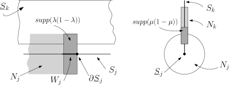
Figure 9. Two sectional views of the tubes $N_{j}$ and $N_{k}$ in $\mathbb{B}^{n}$.

B.7.

Skew associativity formula. For $j<k$, let $S_{j}$ and $\underline{S}_{\,j}$ be a $j$-dimensional stratum of the cone $C\subset\mathbb{B}^{n}$ and its compact subdomain; and let $\lambda:\underline{S}_{\,j}\to[0,1]$ be a balancing function for $S_{j}$. The position of $S_{\,j}$ with respect to $S_{\,k}$ is specified in subsection 3.5 (see Figure 9). If $N_{j,x}$ is a fiber of $N_{j}$, with $x\in\underline{S}_{\,j}$, and $y$ is a point in $N_{j,x}\cap W_{k}$, the fiber $N_{k,y}$ is an affine subspace of $N_{j,x}$. Then, the reducing process with respect to stratum $S_{k}\cap N_{j,x}$ may be applied to the translation vector $u^{j}_{\mathfrak{v}}$ in the $(n-j)$-ball $N_{j,x}$. One gets the next fomula along the fiber $N_{k,y}\subset N_{j,x}$:

(B.9) $$u^{k}_{\mathfrak{v}}=\left(u^{j}_{\mathfrak{v}}\right)^{k}_{\mathfrak{v}}\quad\text{and}\quad u^{k}_{\mathfrak{h}}=u^{j}_{\mathfrak{h}}+\left(u^{j}_{\mathfrak{h}}\right)^{k}_{\mathfrak{h}}\text{ that is,}$$

$$u^{k}_{\mu}=\mu\lambda\,u^{j}_{\mathfrak{h}}+\mu\left(u^{j}_{\mathfrak{h}}\right)^{k}_{\mathfrak{h}}+\left(u^{j}_{\mathfrak{v}}\right)^{k}_{\mathfrak{v}}.$$

Note these formulas hold regardless of the functions $\lambda$ and $\mu$. The subscript $\mathfrak{h}$ has two different meanings: one stands for parallelism to $T_{x}S_{j}$ and the second one for parallelism in $N_{j,x}$ to $T_{y}\bigl{(}S_{k}\cap N_{j,x}\bigr{)}$.

There are analogous formulas associated with a sequence of strata $S_{j_{1}},S_{j_{2}},...,S_{j_{r}}$ when each is in the closure of the next one.

Proposition B.8.

In the setting of Corollary B.2 of a stratified cone $C\in\mathbb{B}^{n}$, it is assumed that the conic transverse structure to each stratum has a global trivialization. If $u$ generates a flow of immediate transversality to $C$ then we have:

1. The reduction $u^{k}_{\mathfrak{v}}$ of $u$ to $N_{k}$ generates a flow of immediate transversality to $C\cap N_{k}$.

2. The flow generated by the balanced reduction of $u$ to $N_{k}$ is of immediate transversality to $C\cap E_{k}$.

Proof. The matter deals with bi-1-jets of $C$ (or pairs of tangent planes to $C$.) This allows one to linearize the considered vector field at any desired point without changing the problem.

On the linear disc bundle $N_{k}$ we have two linear connections $h_{0}$ and $h_{1}$ (seen as plane distributions complementary to the fibers): $h_{0}$ is parallel to $T_{x}S_{k}$ along the fiber $N_{k,x}$ for every $x\in S_{k}$; and $h_{1}$ is given by the assumed global trivialization of $N_{k}$. The difference between them, seen as a vertical deviation, is measured by a 1-form $\omega$ on $S_{k}$ valued in the vector space of linear endomorphisms of the vector bundle spanned by $N_{k}$.

By assumption, the vector $u$ generates a translation flow of immediate transversality to $C$. Let $\alpha$ be the minimum angle between $T_{y}C$ and a hyperplane containing $T_{y+tu}C$ for every $y\in C$ and small positive $t$. The lowest bound of this angle is positive by assumption on $u$; it is independent of $t$ since $C$ is a cone and it is a minimum since $C$ has a compact base.

Claim. If $h_{0}=h_{1}$, then the statement holds.

Indeed, by the above assumption the distribution $h_{0}$ is tangent to $C$. Then, transversality to $C$ translates to the vertical component of the flow of $u$. By an order-one Taylor expansion at $y\in C$, an “infinitesimal contact”, namely coplanarity of $D_{y}(u^{k}_{\mathfrak{v}})(T_{y}C)$ to $T_{y}C$, implies at most transversality to $C$ with an arbitrarily small angle for some small $t>0$, contradicting $\alpha>0$. This proves (1) in this setting. If (2) fails, it should fail infinitesimally which is impossible by (1). $\Box$

Let $y\in N_{k,x}$ and let $y+tu^{k}_{\mathfrak{v}}(x)$ be the vertically displaced point for a small time $t$; suppose both points belong to $C$. The planes $h_{1}(y)$ and $h_{1}(y+tu^{k}_{\mathfrak{v}}(x))$ are both tangent to $C$ but could be not parallel anymore. Nevertheless, thanks to the 1-form $\omega$ which measures the “difference $h_{1}-h_{0}$”, one computes that the angle between $h_{1}(y)$ and $h_{1}(y+tu^{k}_{\mathfrak{v}}(x))$, the latter being translated to $y$, is a $O(t)$. Therefore, if $t>0$ is sufficiently small, this angle is negligible with respect to $\alpha$. So, the reasoning for the claim still holds.

$\Box$

Appendix C Basics on homotopical algebras

In this appendix we review the basic terminology and result of the theory of $A_{\infty}$-algebras. We refer the reader to Kenji Lefèvre-Hasegawa’s thesis [16] for a comprehensive treatment. However, here we use the sign convention introduced [12].

Here, $\bf{k}$ is a unitary ring.

Definition C.1.

An $A_{p}$-algebra is a $\bf{k}$-module equipped with a collection of $\bf{k}$-module maps $m_{i}:A^{\otimes i}\to A$, $1\leq i\leq p$ , of degree $2-i$ satisfying the identities

(C.1) $$\sum_{j+k+l=i}(-1)^{j+kl}m_{j+l+1}(1^{\otimes j}\otimes m_{k}\otimes 1^{\otimes l})=0$$

for all $p\geq i\geq 1$.

Similarly an $A_{\infty}$-algebra is a graded $\bf{k}$-module $A$ together with a collection of $\bf{k}$-module maps $m_{i}:A^{\otimes i}\to A$, $i\geq 1$ , of degree $2-i$ such for all $p$ , $(A,\{m_{i}\}_{1\leq i\leq p})$ is an $A_{p}$-algebra.

Remark C.2.

According to the sign convention in [16] one should put $(-1)^{jk+l}$ instead of $(-1)^{j+kl}$. It turns out that these two definitions are equivalent. Indeed if $(m_{1},m_{2},\cdots)$ is an $A_{\infty}$-structure according to the sign convention of [16], then $(m_{1},(-1)^{2\choose 2}m_{2},\cdots(-1)^{i\choose 2}m_{i},\cdots)$ is an $A_{\infty}$-structure by our sign convention. The sign conventions in [16] is justified by the cobar construction. The signs in [12] correspond to that of the opposite algebra in [16].

Let $(A,\{m_{i}\}_{1\leq i\leq p})$ and $(A^{\prime},\{m^{\prime}_{i}\}_{1\leq i\leq p})$ be two $A_{p}$-algebras. An $A_{p}$-morphism from $(A,\{m_{i}\}_{1\leq i\leq p})$ to $(A^{\prime},\{m^{\prime}_{i}\}_{1\leq i\leq p})$ consists of a collection of maps $f_{i}:A^{\otimes i}\to A^{\prime}$, $1\leq i\leq p$, with the $|f_{i}|=1-i$ satisfying the conditions

(C.2) $$\sum_{j+k+l=i}(-1)^{{j+kl}}f_{j+l+1}\ (1^{\otimes j}\otimes m_{k}\otimes 1^{\otimes l})=\sum_{k=1}^{i}\sum_{i_{1}+\cdots+i_{k}=i}(-1)^{\epsilon_{i_{1},\cdots i_{k}}}m^{\prime}_{k}(f_{i_{1}}\otimes\cdots\otimes f_{i_{k}})\\$$

where $\epsilon_{i_{1},\cdots i_{k}}=\sum_{j=1}^{k}(k-j)(i_{j}-1)$.

Remark C.3.

If we follow the sign convention of [16], then equation of C.2 transforms into

(C.3) $$\sum_{j+k+l=i}(-1)^{l+jk}f_{j+l+1}\ (1^{\otimes j}\otimes m_{k}\otimes 1^{\otimes l})=\sum_{k=1}^{i}\sum_{i_{1}+\cdots+i_{k}=i}(-1)^{\epsilon_{i_{1},\cdots i_{k}}}m^{\prime}_{k}(f_{i_{1}}\otimes\cdots\otimes f_{i_{k}})\\$$

where $\epsilon_{i_{1},\cdots i_{k}}=\sum_{j}((1-i_{j})\sum_{1\leq k\leq j}i_{k})$.

If $(m_{i})$ and $(f_{i})$ satisfy the equation (C.2), then $(m_{1},(-1)^{2\choose 2}m_{2},\cdots(-1)^{i\choose 2}m_{i},\cdots)$ and

$$(f_{1},(-1)^{2\choose 2}f_{2},\cdots(-1)^{i\choose 2}f_{i},\cdots)$$

satisfies (C.3).

A collection of $\bf{k}$-module maps $f=\{f_{i}\}_{i\geq 1}:A^{\otimes i}\to A^{\prime}$ is said to be a morphism of $A_{\infty}$-algebras if for all $p$, $\{f_{i}\}_{1\leq i\leq p}$ is a morphism of $A_{p}$-algebras.

An $A_{\infty}$-morphism $f=\{f_{i}\}_{i\geq 1}$ is said to be a quasi-isomorphism if the cochain complex map $f_{1}$ is a quasi-isomorphism.

Definition C.4.

Let $A$ and $A^{\prime}$ be two $A_{\infty}$-algebras with the corresponding differentials $D$ and $D^{\prime}$ on the bar constructions $BA$ and $BA^{\prime}$. Suppose that $f=\{f_{i}\},g=\{g_{i}\}:A\to A^{\prime}$ are two $A_{\infty}$-morphisms and $F$ and $G$ are the coalgebra morphisms corresponding to $f$ and $g$. Then a homotopy between $f$ and $g$ is a $(F,G)$-coderivation $H:BA\to BA^{\prime}$ such that

(C.4) $$F-G=D^{\prime}H-HD.$$

Theorem C.5.

(Prouté [21], see also [16].) We suppose that $\bf{k}$ is a field. Then we have:

1. For connected $A_{\infty}$-algebras, homotopy is an equivalence relation (Theorem 4.27).

2. A quasi-isomorphism of $A_{\infty}$-algebras is a homotopy equivalence (Theorem 4.24).

References

- [1] Abouzaid M., A topological model for the Fukaya categories of plumbings. J. Differential Geom. 87 (2011), no. 1, 1-80.
- [2] Betz M., Cohen R., Graph Moduli Spaces and Cohomology Operations, Turkish J. Math. 18 (1995), 23-41.
- [3] Chang K.C., Liu J., A cohomology complex for manifolds with boundary, Top. Methods in Non Linear Analysis 5 (1995), 325 - 340.
- [4] Charest F., Woodward C.T., Floer theory and flips, 171 pages, arXiv:1508.01573.
- [5] Conley C., Isolated invariant sets and the Morse index, CBMS Reg. Conf. Series in Math., vol. 38, A.M.S., Providence, R.I., 1978.
- [6] Cornea O., Ranicki A., Rigidity and gluing for Morse and Novikov complexes. J. Eur. Math. Soc. (JEMS) 5 (2003), no. 4, 343-394.
- [7] Floer A., Morse theory for Lagrangian intersections, J. Differential Geom. 28 n∘ 3 (1988), 513-547.
- [8] Fukaya K., Morse homotopy, -categories, and Floer homologies, Proc. of GARC workshop on Geometry and Topology, (H.J. Kim, ed.), Seoul National University (1993), 1-102.
- [9] Harvey F.R., Lawson H.B., Finite volume flows and Morse theory, Annals of Math. 153 (2001), 1-25.
- [10] Helffer B., Nier F., Quantitative analysis of metastability in reversible processes via a Witten complex approach: the case with boundary, Mém. Soc. Math. Fr. 105 (2006).
- [11] Hutchings M., Floer homology of families. I. Algebr. Geom. Topol. 8 (2008), no. 1, 435-492.
- [12] Keller B. , Introduction to -infinity Algebras and modules, Homology Homotopy Appl. 3 (1) (2001), 1 - 35.
- [13] Koldan N., Prokhorenkov I., Shubin M., Semiclassical asymptotics on manifolds with boundary, in: Spectral analysis in geometry and number theory, 239–266, Contemp. Math., 484, Amer. Math. Soc., 2009.
- [14] Laudenbach F., On the Thom-Smale complex, Appendix to: J.-M. Bismut - W. Zang, An extension of a Theorem by Cheeger and Müller, Astérisque 205 (1992), 219-233.
- [15] Laudenbach F., A Morse complex on manifolds with boundary, Geometriae Dedicata, vol. 153 (1) (2011), 47-57.
- [16] Lefevre-Hasegawa K., Sur les -categories, Thèse de doctorat sous la direction de Bernhard Keller, Paris 7, 2003 (available at https://arxiv.org/abs/math/0310337).
- [17] Mazuir T., Higher algebra of and -algebras in Morse theory I, arXiv:2102.06654.
- [18] Mescher S. Perturbed gradient flow trees and -algebra structures in Morse cohomology, Atlantis Studies in Dynamical Systems, 6, Springer, 2018.
- [19] Milnor J., Lectures on the -cobordism Theorem, Princeton University Press, 1965.
- [20] Morse M., Van Schaack G.B., The critical point theory under general boundary conditions, Annals of Math. 35 n∘ 3 (1934), 545-571.
- [21] Prouté A., -structures. Modèles minimaux de Baues-Lemaire et Kadeishvili et homologie des fibrations, Reprint of the 1986 original with a preface to the reprint by Jean-Louis Loday, Repr. Theory Appl. Categ. No. 21 (2011), 1-99.
- [22] Seidel P., Fukaya categories and Picard-Lefschetz theory, Zurich Lectures in Advanced Mathematics. European Mathematical Society (EMS), Zürich, 2008.
- [23] Schwarz M., Equivalences for Morse homology Geometry and topology in dynamics, 197-216, Contemp. Math., 246, Amer. Math. Soc., Providence, RI, 1999.
- [24] Thom R., Quelques propriétés globales des variétés différentiables, Comment. Math. Helv. 28 (1954), 17-86.
- [25] Thom R., Un lemme sur les applications différentiables, Boletin de la Sociedad Matemàtica Mexicana (2) 1 (1956), 59-71.
- [26] Watanabe T., Higher order generalization of Fukaya’s Morse homotopy invariant of 3-manifolds I. Invariants of homology 3-spheres, Asian J. Math. 22 (2018), no. 1, 111-180.