Effective temperature of ionizing stars of extragalactic H ii regions–II: nebular parameter relations based on CALIFA data

Abstract

We calculate the effective temperature ($T_{\rm eff}$) of ionizing star(s), oxygen abundance of the gas phase $(\rm O/H)$, and the ionization parameter $U$ for a sample of H ii regions located in the disks of 59 spiral galaxies in the $0.005\><\>z\><\>0.03$ redshift range. We use spectroscopic data taken from the CALIFA data release 3 (DR3) and theoretical (for $T_{\rm eff}$ and $U$) and empirical (for O/H) calibrations based on strong emission-lines. We consider spatial distribution and radial gradients of those parameters in each galactic disk for the objects in our sample. Most of the galaxies in our sample ($\sim 70$ %) shows positive $T_{\rm eff}$ radial gradients even though some them exhibit negative or flat ones. The median value of the $T_{\rm eff}$ radial gradient is 0.762 kK/$R_{25}$. We find that radial gradients of both $\log U$ and $T_{\rm eff}$ depend on the oxygen abundance gradient, in the sense that the gradient of $\log U$ increases as $\log(\rm O/H)$ gradient increases while there is an anti-correlation between the gradient of $T_{\rm eff}$ and the oxygen abundance gradient. Moreover, galaxies with flat oxygen abundance gradients tend to have flat $\log U$ and $T_{\rm eff}$ gradients as well. Although our results are in agreement with the idea of the existence of positive $T_{\rm eff}$ gradients along the disk of the majority of spiral galaxies, this seems not to be an universal property for these objects.

1 Introduction

The determination of the effective temperature ($T_{\rm eff}$) of the ionizing star(s) belonging to H ii regions is crucial to understand the processes that restrict the formation and evolution of massive stars, the physics of stellar atmosphere, the excitation of the Interstellar Medium (ISM) as well as the galaxy in which they reside.

For ionizing stars of nearby H ii regions, located in the Milky Way and the Magellanic Clouds, the effective temperature can be directly estimated by using their photometric and spectrometric data (e.g. Massey et al. 2005; Massey et al. 2009; Corti et al. 2007; Sota et al. 2011; Morrell et al. 2014; Walborn et al. 2014; Lamb et al. 2016; Evans et al. 2015; Mohr-Smith et al. 2017; Martins & Palacios 2017; Markova et al. 2018). However, for the majority of the distant ionizing massive stars, $T_{\rm eff}$ can only be indirectly estimated, e.g. from the analysis of emission-lines emitted by the nebulae ionized by these stars. By using this methodology, proposed by Zanstra (1929), it is possible to estimate $T_{\rm eff}$ and its behaviour along the disk of spiral galaxies (see e.g. Dors et al. 2017 and references therein).

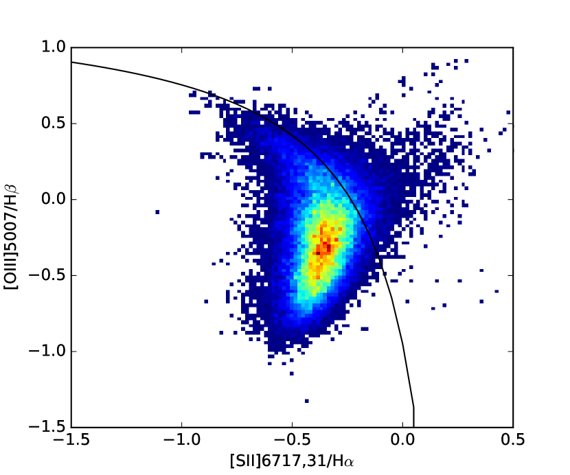
Figure 1: BPT diagnostic diagram (Baldwin et al., 1981) for all the spaxels in our sample. The solid line is the boundary between AGN-like and H ii-like regions defined by Kewley et al. (2001).

Due to effects of opacity and/or line-blanketing in the stellar atmospheres (Abbott & Hummer, 1985; Schaerer & Schmutz, 1994; Martins et al., 2005), stars with higher metallicity ($Z$) trend to present lower values of $T_{\rm eff}$ than their counterparts with the same mass but lower $Z$ (e.g. Mokiem et al. 2004; Martins et al. 2004). It is well known that spiral galaxies exhibit metallicity gradients, in the sense that $Z$ decreases with the increment of the galactocentric radius (e.g. Pilyugin et al. 2004). Therefore, assuming that stars are formed with an universal stellar upper mass limit of the Initial Mass Function (e.g. Bastian et al. 2010), it is expected a positive gradient of $T_{\rm eff}$ in the disks of spiral galaxies. In fact, Shields & Searle (1978) interpreted that the enhancement of the equivalent width of the H$\beta$ emission-line with the galactocentric distance for a sample of H ii regions in M 101 could be due to a positive $T_{\rm eff}$ gradient (see also Vilchez & Pagel 1988; Henry & Howard 1995; Dors & Copetti 2003, 2005). In spite of these gradients should exist in most of the spiral galaxies, they were not found in early studies (e.g. Fierro et al. 1986; Evans 1986). Recently, Dors et al. (2017) studied the $T_{\rm eff}$ variation as a function of the galactocentric distance for H ii regions belonging to 14 spiral galaxies using a new theoretical calibration between the observed emission-line ratio $R$=log([O ii]($\lambda$$\lambda$3726+29)/[O iii]$\lambda$5007) and $T_{\rm eff}$ (relation proposed by Dors & Copetti, 2003). These authors found positive gradients for 11 of these galaxies, null gradients for two and a negative gradient for the other one (see also Pérez-Montero & Vílchez 2009). In particular, the first negative $T_{\rm eff}$ gradient was found for the Milky Way by Morisset (2004). Additional analysis taking into account a larger number of galaxies is necessary to ascertain if the $T_{\rm eff}$ gradient is an universal property of spiral galaxies.

The knowledge of the relation between different physical parameters is essential to comprehend which mechanisms drive the formation and evolution of galaxies. For example, in the seminal paper, Lequeux et al. (1979) calculated the metallicity (traced by the ratio between oxygen and hydrogen abundances) and the total galaxy mass ($M_{\rm T}$; obtained from atomic hydrogen velocity maps) for eight irregular and blue compact galaxies and found a clear relation between these parameters (see also Kinman & Davidson 1981; Peimbert & Serrano 1982; Rubin et al. 1984; Skillman 1992; Tremonti et al. 2004; Pilyugin et al. 2004; Sánchez et al. 2013, among others). Thereafter, Ellison et al. (2008) showed that the $M_{\rm T}$-$Z$ relation is affected by a dependence of the metallicity on the star formation rate (SFR), establishing the $M_{\rm T}$-$Z$-SFR relation. This result was confirmed by Lara-López et al. (2010); Mannucci et al. (2010). However, Sánchez et al. (2017) in their recent study, based on integral field spectroscopy data, did not find any significant dependence of the $M_{\rm T}$-$Z$ relation with the SFR, but they did not exclude the existence of such relation on local scales, e.g. in the central regions of the galaxies. Therefore, the existence of the universality of $T_{\rm eff}$ gradients, together with the $M_{\rm T}$-$Z$-SFR relation, would produce additional and fundamental concepts of the physical processes taking place in galaxies, important insights into how the formation and evolution of massive stars occur as well as their interaction with the ISM.

In this work, we use the methodology presented by (Dors et al., 2017, hereafter Paper I), to estimate $T_{\rm eff}$ of extragalactic H ii regions located in a large sample of spiral galaxies. We have taken advantage of the existence of an homogeneous sample of spectroscopic data of H ii regions obtained as part of the Calar Alto Legacy Integral Field Area Survey (CALIFA, Sánchez et al. 2012), which is ideal to investigate global scaling relations between galaxy properties (see e.g. Ellison et al. 2018). The main goals of the present study are to investigate if $T_{\rm eff}$ gradients are universal properties of spiral galaxies, and the existence of any correlation between $T_{\rm eff}$ and nebular parameters such as the ionization parameter or the oxygen abundance. This paper is organized as follows. The methodology assumed to calculate $T_{\rm eff}$ and the observational data used along this work are described in Sec. 2. In Sect. 3 the results and discussion of the outcome are presented. Finally, conclusions are given in Sect. 4.

2 Methodology

2.1 Sample

We used publicly available spectra from the integral field spectroscopic CALIFA survey data release 3 (DR3; Sánchez et al., 2016, 2012; Walcher et al., 2014) based on observations with the PMAS/PPAK integral field spectrophotometer mounted on the Calar Alto 3.5-meter telescope. CALIFA DR3 provides wide-field IFU data for 667 objects in total. The data for each galaxy consist of two datacubes, which cover the spectral regions of 4300–7000 $\AA$ at a spectral resolution of $R\sim 850$ (setup V500) and of 3700–5000 $\AA$ at $R\sim 1650$ (setup V1200). For the galaxies with both V500 and V1200 datacubes available, there are COMB datacubes for 446 galaxies which are a combination of V500 and V1200 datacubes covering the 3700–7000 $\AA$ spectral range. In this study we used these COMB datacubes.

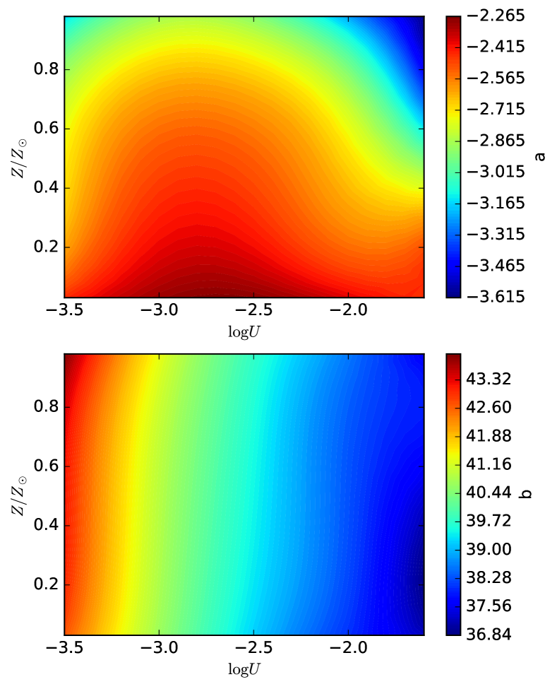
Figure 2: Coefficients $a$ (upper panel) and $b$ (lower panel) of the linear regression $T_{\rm eff}=a\times R+b$ as a function of $\log U$ and $Z/Z_{\odot}$.

The sample of galaxies is described in detail in Zinchenko et al. (2018, in prep.). Briefly, we selected isolated galaxies with inclination less than $60\degree$. Galaxies with insufficient number of spaxels with measured oxygen abundance were excluded from our sample. We also rejected from our sample galaxies with oxygen abundance measurements for less than 50 spaxels and/or galaxies for which spaxels with oxygen abundance measurements cover a range of galactocentric distances lower than $\sim$ 1/3 of the its optical radius. Stellar masses, derived from UV-to-NIR photometry, has been taken from Walcher et al. (2014). Our final sample contains 59 galaxies and 49067 spaxels.

The final spatial resolution of the CALIFA data is set by the fiber size of the PMAS/PPAK integral field spectrophotometer and it is of the order of 3 arcsec (Husemann et al., 2013). Thus, the spectrum of each spaxel corresponds to the spectrum emitted by a region with a diameter varying from $\sim$300 pc to $\sim$1.5 kpc depending on the distance to the galaxy. Therefore, each observed spectrum comprises the flux of a complex of H ii regions and the physical properties derived represent an averaged value (see discussion in Paper I).

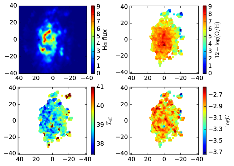
Figure 3: Maps of the H$\alpha$ emission-line flux (top-left panel), oxygen abundance (top-right panel), $T_{\rm eff}$ (bottom-left panel), and $\log U$ (bottom-right panel) for NGC 237.

2.2 The emission line fluxes

The spectrum of each spaxel from the CALIFA DR3 datacubes is processed in the same way as described in Zinchenko et al. (2016). Briefly, the stellar background in all spaxels is fitted using the public version of the STARLIGHT code (Cid Fernandes et al., 2005; Mateus et al., 2006; Asari et al., 2007) adapted for execution in the NorduGrid ARC environment of the Ukrainian National Grid. To fit the stellar spectra we used 45 synthetic simple stellar population (SSP) spectra from the evolutionary synthesis models by Bruzual & Charlot (2003) with ages from 1 Myr up to 13 Gyr and metallicities $Z=0.004$, 0.02, and 0.05. We adopted the reddening law of Cardelli et al. (1989) with $R_{V}=3.1$. The resulting stellar radiation contribution is subtracted from the observed spectrum in order to measure and analyse the line emission from the gaseous component. The line intensities were measured using single Gaussian line profile fittings on the pure emission spectra.

The total [O iii]$\lambda$$\lambda$4959,5007 flux has been estimated as $1.33\>\times$ [O iii]$\lambda$5007 instead of as the sum of the fluxes of both lines. These lines originate from transitions from the same energy level, so their flux ratio can be determined by the transition probability ratio, which is very close to 3 (Storey & Zeippen, 2000). The strongest line, [O iii]$\lambda$5007, can be measured with higher precision than the weakest one. This is particularly important for high-metallicity H ii regions, which have weak high-excitation emission-lines. Similarly, the [N ii]$\lambda$$\lambda$6548,6584 lines also originate from transitions from the same energy level and the transition probability ratio for those lines is again close to 3 (Storey & Zeippen, 2000). Therefore, we estimated its total flux as $1.33$ [N ii]$\lambda$6584. For each spectrum, we measure the fluxes of the [O ii]$\lambda\,\lambda$3727,3729, H$\beta$, [O iii]$\lambda$5007, H$\alpha$, [N ii]$\lambda$6584, and [S ii]$\lambda$6717, 6731. For the further analysis we selected only those spectra, for which the signal-to-noise ratio is larger than $5$ for each emission-line listed above. The measured line fluxes are corrected for interstellar reddening using the theoretical H$\alpha$ to H$\beta$ ratio assuming the standard value of H$\alpha$/H$\beta$ = 2.86, and the analytical approximation of the Whitford interstellar reddening law from Izotov et al. (1994). When the measured value of H$\alpha$/H$\beta$ is lower than 2.86 the reddening is adopted to be zero.

Following Paper I, we apply the $\log$([O iii]$\lambda$5007/H$\beta$) – $\log$([S ii]$\lambda\lambda$6717,6731/H$\alpha$) criterion proposed by Kewley et al. (2001) to separate objects for which the main ionization source are massive stars from those whose main ionization source are shocks of gas and/or active galactic nuclei (AGNs). We consider only the objects located below the separation line defined by Kewley et al. (2001), i.e. 39431 spaxels. In Fig. 1, the BPT diagnostic diagram (Baldwin et al., 1981) for the all the spaxels in our sample is presented.

2.3 Nebular parameter determinations

In order to estimate $T_{\rm eff}$, we adopted the same method proposed in Paper I, where a new calibration between $T_{\rm eff}$ and the $R$ = $\log$([O ii]$\lambda\lambda$3727,3729/[O iii]$\lambda$5007) ratio was proposed. The method consists of three steps: a) to estimate the metallicity $Z$ of star forming regions, b) to estimate $U$ from $Z$ and [S ii]$\lambda\lambda$6717,6731 and H$\alpha$ emission lines, and c) to estimate $T_{\rm eff}$ from $U$, $Z$, and $R$.

Entering into details, the first step consists in calculating the metallicity of the gas traced by the oxygen abundance in relation to the hydrogen one, in units of 12+$\log(\rm O/H)$. It is carried out using the R_3D empirical calibration given by Pilyugin & Grebel (2016). These authors derived oxygen abundances based on direct estimations of the electron temperatures for a large sample of H ii regions and they obtained relations between these abundances and the emission line flux ratios of oxygen and nitrogen in relation to H$\beta$ defined as: $R_{2}=$[O ii]$\lambda\lambda$3727,3729/H$\beta$, $R_{3}=$[O iii]$\lambda\lambda$4959,5007/H$\beta$, $N_{2}=$[N ii]$\lambda\lambda$6548,6584/H$\beta$. To use this calibration it is necessary to define which branch of the curve must be considered, due to the degeneracy in the calibrations. For H ii regions with $\log N_{2}\geq-0.6$ the upper branch is assumed and the relation is the following:

$$\begin{array}[]{lll}{\rm(O/H)}_{R,U}&=&8.589+0.022\,\log(R_{3}/R_{2})+0.399\,\log N_{2}\\ &+&(-0.137+0.164\,\log(R_{3}/R_{2})+0.589\log N_{2})\\ &\times&\log R_{2},\\ \end{array}$$ (4)

where (O/H)_R,U means 12 +log(O/H)_R,U.

For H ii regions with $\log N_{2}<-0.6$, the lower branch is assumed and the relation is

$$\begin{array}[]{lll}{\rm(O/H)}_{R,L}&=&7.932+0.944\,\log(R_{3}/R_{2})+0.695\,\log N_{2}\\ &+&(0.970-0.291\,\log(R_{3}/R_{2})-0.019\log N_{2})\\ &\times&\log R_{2},\\ \end{array}$$ (8)

where (O/H)_R,L means 12 +log(O/H)_R,L. To convert the oxygen abundance to metallicity $Z/Z_{\odot}$, we assumed the solar oxygen abundance 12+$\log(\rm O/H)_{\odot}=8.69$ (Allende Prieto et al., 2001).

Following Paper I, the logarithm of the ionization parameter, $\log U$, is calculated as:

$$\log U=c\times S2+d,$$ (9)

where $S2$ = $\log$([S ii]$\lambda\lambda$6717,6731/H$\alpha$), $c=-0.26\times(Z/Z_{\odot})-1.54$, and $d=-3.69\times(Z/Z_{\odot})^{2}+5.11\times(Z/Z_{\odot})-5.26$.

The $T_{\rm eff}$-$R$ relation derived in Paper I is

$$T_{\rm eff}=a\times R+b,$$ (10)

where $R$ = $\log$([O ii]$\lambda\lambda$3727,3729/[O iii]$\lambda$5007). Fig. 2 shows the values of the $a$ and $b$ coefficients as a function of $Z/Z_{\odot}$ and $\log U$. In this figure, the values of the coefficients are calculated interpolating the relations given in Table 2 of Paper I.

It is worth to mention that the expected maximum effective temperature of a young stellar cluster is $\sim$ 50 kK (e.g., Martins et al., 2005; Simón-Díaz et al., 2014; Tramper et al., 2014; Walborn et al., 2014; Wright et al., 2015; Crowther et al., 2016; Martins & Palacios, 2017; Holgado et al., 2018) Meanwhile, the $T_{\rm eff}-R$ relation can be applied only for $T_{\rm eff}\lid 40$ kK because, for higher $T_{\rm eff}$ values, small variations of $R$ produce extremely large uncertainties in $T_{\rm eff}$ estimations (Dors et al., 2017). Kennicutt et al. (2000) derived a calibration between $T_{\rm eff}$ and the He ii$\lambda$5876/H$\beta$ and He ii$\lambda$6678/H$\beta$ emission-line ratios, and they also pointed out a similar difficulty in deriving effective temperature values higher than $\sim$40kK. Thus, in this study we consider only objects for which we derive a $T_{\rm eff}$ value lower or equal to 40 kK. It should also be noted that $T_{\rm eff}$ values higher than 40 kK were derived only for about 15% of the H ii regions in our sample. Fig. 3 shows an example of the obtained maps for the H$\alpha$ emission line flux, oxygen abundance, $T_{\rm eff}$, and $\log U$ for one of the galaxies in our sample (NGC 237).

2.4 Radial gradients

Using the methodology and the observational data presented above, we calculate radial gradients for $T_{\rm eff}$, $\log U$ and $12+\log({\rm O/H})$ along the disk of the galaxies in our sample. For each galaxy, we fitted the radial distributions of these parameters by the use of the following relation:

$$Y=Y_{0}+grad\,Y\times R/R_{25},$$ (11)

where $Y$ is a given parameter, $Y_{0}$ is the extrapolated value of this parameter to the galactic center, $grad\,Y$ is the slope of the distribution expressed in Y units per optical radius $R_{25}$. The radial gradients were estimated using the data in galactocentric distances $0.2\>R_{25}\><\>R\><\>R_{25}$.

In Fig. 4, an example of the radial gradients of $T_{\rm eff}$, $\log U$, and $12+\log({\rm O/H})$ is presented for the spiral galaxy NGC 2730. This galaxy has a clear positive radial gradient of $T_{\rm eff}$ and negative radial gradients of $\log U$ and $12+\log({\rm O/H})$. Same plots for the radial gradients together with the $12+\log({\rm O/H})$ vs. $\log U$, $12+\log({\rm O/H})$ vs. $T_{\rm eff}$ diagrams for each galaxy in our sample are available in a supplementary material.

Table 1 presents our sample of galaxies and the best fit of the radial distribution of $T_{\rm eff}$, $\log U$ and $12+\log({\rm O/H})$ for each galaxy.

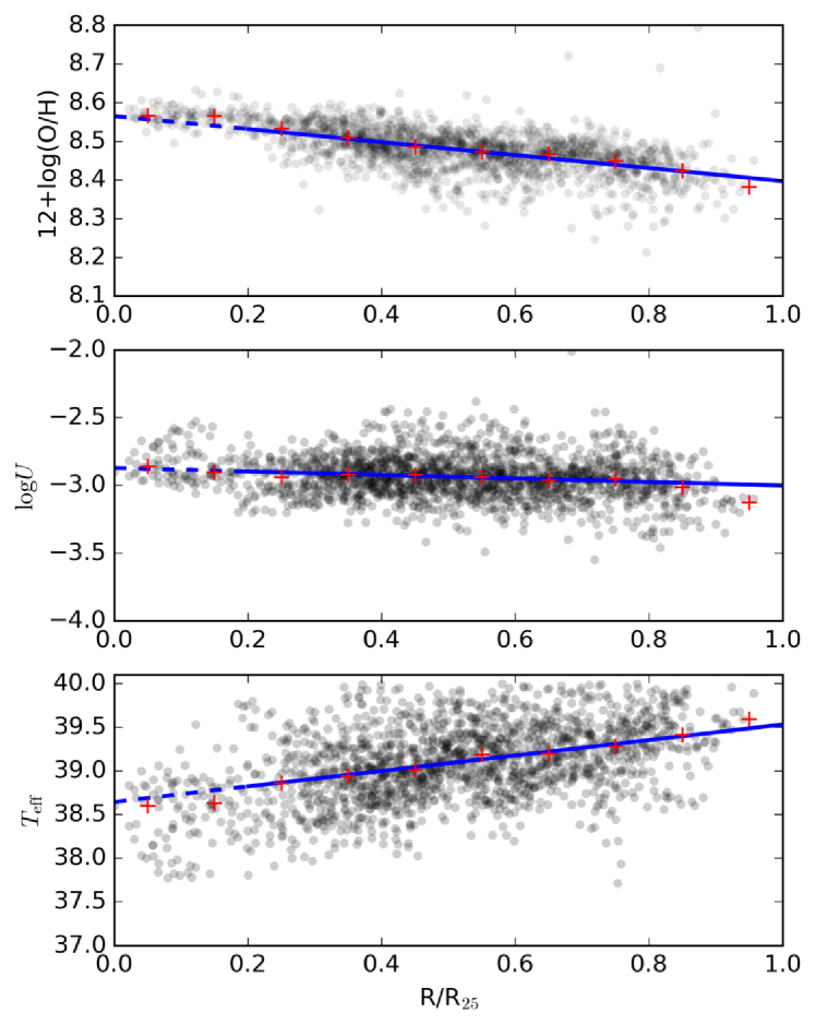
Figure 4: Radial gradients of effective temperature ($T_{\rm eff}$), logarithm of the ionization parameter ($\log U$) and of oxygen abundance (12+log(O/H) for NGC 2730, one galaxy of the CALIFA sample. The gray filled circles represent the observational data. The blue solid line is the best fit for the data, the blue dashed line is the extrapolation to the center. The red plus signs are median values in bins of 0.1 $R_{25}$.

Table 1: List of the selected galaxies from the CALIFA survey

Name	$12+\log({\rm O/H})_{0}$	grad $\log({\rm O/H})$	$\log U$	grad $\log U$	$T_{\rm eff}$	grad $T_{\rm eff}$
	dex	dex/$R_{25}$	dex	dex/$R_{25}$	kK	kK/$R_{25}$
NGC 1	8.615 $\pm$ 0.006	-0.029 $\pm$ 0.012	-2.865 $\pm$ 0.026	0.073 $\pm$ 0.052	38.802 $\pm$ 0.120	-0.317 $\pm$ 0.234
NGC 23	8.730 $\pm$ 0.010	-0.209 $\pm$ 0.024	-3.400 $\pm$ 0.058	0.751 $\pm$ 0.146	39.393 $\pm$ 0.160	-0.734 $\pm$ 0.369
NGC 180	8.705 $\pm$ 0.034	-0.217 $\pm$ 0.049	-2.629 $\pm$ 0.083	-0.038 $\pm$ 0.120	38.088 $\pm$ 0.337	0.380 $\pm$ 0.484
NGC 234	8.617 $\pm$ 0.004	-0.062 $\pm$ 0.009	-2.696 $\pm$ 0.014	-0.382 $\pm$ 0.032	37.938 $\pm$ 0.071	1.205 $\pm$ 0.161
NGC 237	8.680 $\pm$ 0.003	-0.317 $\pm$ 0.007	-2.835 $\pm$ 0.011	-0.165 $\pm$ 0.023	38.139 $\pm$ 0.038	1.405 $\pm$ 0.077
NGC 257	8.696 $\pm$ 0.014	-0.255 $\pm$ 0.021	-2.806 $\pm$ 0.044	0.020 $\pm$ 0.068	38.152 $\pm$ 0.160	0.585 $\pm$ 0.248
NGC 309	8.781 $\pm$ 0.015	-0.432 $\pm$ 0.030	-2.503 $\pm$ 0.066	-0.435 $\pm$ 0.133	36.933 $\pm$ 0.218	2.893 $\pm$ 0.439
NGC 477	8.543 $\pm$ 0.010	-0.058 $\pm$ 0.014	-2.717 $\pm$ 0.025	-0.201 $\pm$ 0.034	38.193 $\pm$ 0.085	0.830 $\pm$ 0.116
NGC 776	8.647 $\pm$ 0.007	0.002 $\pm$ 0.014	-2.826 $\pm$ 0.048	0.198 $\pm$ 0.101	38.149 $\pm$ 0.210	0.516 $\pm$ 0.440
NGC 941	8.561 $\pm$ 0.006	-0.394 $\pm$ 0.015	-2.816 $\pm$ 0.018	-0.410 $\pm$ 0.047	38.698 $\pm$ 0.050	1.328 $\pm$ 0.134
NGC 991	8.532 $\pm$ 0.008	-0.269 $\pm$ 0.019	-2.951 $\pm$ 0.028	-0.034 $\pm$ 0.067	38.945 $\pm$ 0.067	0.515 $\pm$ 0.163
NGC 1070	8.626 $\pm$ 0.032	-0.035 $\pm$ 0.111	-2.673 $\pm$ 0.103	-0.150 $\pm$ 0.349	38.754 $\pm$ 0.492	-1.394 $\pm$ 1.669
NGC 1094	8.656 $\pm$ 0.004	-0.117 $\pm$ 0.010	-3.127 $\pm$ 0.021	0.291 $\pm$ 0.052	38.955 $\pm$ 0.070	0.570 $\pm$ 0.170
NGC 1659	8.621 $\pm$ 0.006	-0.184 $\pm$ 0.012	-2.777 $\pm$ 0.017	-0.113 $\pm$ 0.034	38.233 $\pm$ 0.053	0.978 $\pm$ 0.105
NGC 1667	8.657 $\pm$ 0.002	-0.067 $\pm$ 0.005	-2.847 $\pm$ 0.013	-0.084 $\pm$ 0.030	38.702 $\pm$ 0.049	0.059 $\pm$ 0.108
NGC 2347	8.689 $\pm$ 0.007	-0.279 $\pm$ 0.011	-2.860 $\pm$ 0.023	0.013 $\pm$ 0.036	37.968 $\pm$ 0.069	1.601 $\pm$ 0.108
NGC 2487	8.639 $\pm$ 0.064	-0.054 $\pm$ 0.123	-2.706 $\pm$ 0.166	-0.041 $\pm$ 0.318	39.319 $\pm$ 0.992	-1.832 $\pm$ 1.900
NGC 2530	8.557 $\pm$ 0.006	-0.251 $\pm$ 0.010	-2.754 $\pm$ 0.018	-0.259 $\pm$ 0.030	38.098 $\pm$ 0.046	1.788 $\pm$ 0.078
NGC 2540	8.626 $\pm$ 0.004	-0.154 $\pm$ 0.006	-2.904 $\pm$ 0.015	0.003 $\pm$ 0.026	38.434 $\pm$ 0.054	0.715 $\pm$ 0.091
NGC 2604	8.524 $\pm$ 0.008	-0.401 $\pm$ 0.020	-2.834 $\pm$ 0.020	-0.488 $\pm$ 0.048	39.348 $\pm$ 0.042	0.586 $\pm$ 0.112
NGC 2730	8.565 $\pm$ 0.003	-0.167 $\pm$ 0.006	-2.870 $\pm$ 0.012	-0.129 $\pm$ 0.021	38.646 $\pm$ 0.030	0.886 $\pm$ 0.054
NGC 2906	8.643 $\pm$ 0.005	0.001 $\pm$ 0.011	-2.911 $\pm$ 0.031	0.025 $\pm$ 0.063	38.494 $\pm$ 0.132	0.328 $\pm$ 0.265
NGC 2916	8.609 $\pm$ 0.015	-0.108 $\pm$ 0.028	-2.728 $\pm$ 0.043	-0.085 $\pm$ 0.076	37.681 $\pm$ 0.125	1.895 $\pm$ 0.223
NGC 3057	8.318 $\pm$ 0.007	-0.194 $\pm$ 0.014	-3.132 $\pm$ 0.020	-0.110 $\pm$ 0.039	39.899 $\pm$ 0.060	-0.324 $\pm$ 0.126
NGC 3381	8.592 $\pm$ 0.004	-0.226 $\pm$ 0.009	-2.927 $\pm$ 0.012	-0.029 $\pm$ 0.027	38.495 $\pm$ 0.040	1.064 $\pm$ 0.092
NGC 3614	8.651 $\pm$ 0.014	-0.358 $\pm$ 0.032	-2.764 $\pm$ 0.038	-0.272 $\pm$ 0.087	37.984 $\pm$ 0.156	1.789 $\pm$ 0.354
NGC 3687	8.697 $\pm$ 0.003	-0.251 $\pm$ 0.007	-3.040 $\pm$ 0.015	0.368 $\pm$ 0.037	38.918 $\pm$ 0.049	0.052 $\pm$ 0.123
NGC 3811	8.649 $\pm$ 0.003	-0.126 $\pm$ 0.006	-2.861 $\pm$ 0.015	0.040 $\pm$ 0.026	37.983 $\pm$ 0.057	1.382 $\pm$ 0.098
NGC 4961	8.533 $\pm$ 0.005	-0.297 $\pm$ 0.009	-2.887 $\pm$ 0.012	-0.338 $\pm$ 0.022	38.814 $\pm$ 0.033	1.221 $\pm$ 0.070
NGC 5000	8.617 $\pm$ 0.012	-0.075 $\pm$ 0.015	-2.638 $\pm$ 0.087	-0.220 $\pm$ 0.102	37.199 $\pm$ 0.215	1.764 $\pm$ 0.251
NGC 5016	8.711 $\pm$ 0.016	-0.254 $\pm$ 0.029	-2.620 $\pm$ 0.089	-0.281 $\pm$ 0.161	38.128 $\pm$ 0.223	1.188 $\pm$ 0.402
NGC 5205	8.559 $\pm$ 0.033	0.001 $\pm$ 0.065	-2.723 $\pm$ 0.084	0.146 $\pm$ 0.168	37.566 $\pm$ 0.435	0.688 $\pm$ 0.863
NGC 5320	8.637 $\pm$ 0.003	-0.210 $\pm$ 0.006	-2.817 $\pm$ 0.010	-0.121 $\pm$ 0.018	38.334 $\pm$ 0.037	0.762 $\pm$ 0.067
NGC 5406	8.650 $\pm$ 0.009	-0.074 $\pm$ 0.017	-2.516 $\pm$ 0.046	-0.458 $\pm$ 0.084	37.698 $\pm$ 0.166	1.248 $\pm$ 0.305
NGC 5480	8.601 $\pm$ 0.003	-0.089 $\pm$ 0.009	-2.842 $\pm$ 0.015	-0.172 $\pm$ 0.039	38.262 $\pm$ 0.053	1.161 $\pm$ 0.135
NGC 5520	8.620 $\pm$ 0.002	-0.097 $\pm$ 0.004	-2.979 $\pm$ 0.009	0.126 $\pm$ 0.015	38.825 $\pm$ 0.029	0.203 $\pm$ 0.044
NGC 5633	8.675 $\pm$ 0.003	-0.166 $\pm$ 0.006	-2.795 $\pm$ 0.013	-0.235 $\pm$ 0.028	38.295 $\pm$ 0.048	0.972 $\pm$ 0.101
NGC 5720	8.531 $\pm$ 0.030	0.021 $\pm$ 0.041	-2.856 $\pm$ 0.089	-0.105 $\pm$ 0.119	39.715 $\pm$ 0.313	-0.353 $\pm$ 0.420
NGC 5732	8.605 $\pm$ 0.005	-0.180 $\pm$ 0.008	-2.840 $\pm$ 0.012	-0.017 $\pm$ 0.018	38.287 $\pm$ 0.048	0.944 $\pm$ 0.072
NGC 5957	8.688 $\pm$ 0.009	-0.180 $\pm$ 0.019	-2.830 $\pm$ 0.046	0.006 $\pm$ 0.099	38.816 $\pm$ 0.164	-0.403 $\pm$ 0.353
NGC 6004	8.639 $\pm$ 0.007	-0.039 $\pm$ 0.022	-2.647 $\pm$ 0.043	-0.237 $\pm$ 0.120	38.085 $\pm$ 0.173	1.160 $\pm$ 0.487
NGC 6063	8.561 $\pm$ 0.008	-0.065 $\pm$ 0.010	-2.940 $\pm$ 0.019	0.054 $\pm$ 0.025	39.200 $\pm$ 0.063	-0.175 $\pm$ 0.082
NGC 6154	8.619 $\pm$ 0.019	-0.019 $\pm$ 0.025	-2.806 $\pm$ 0.093	-0.153 $\pm$ 0.119	39.245 $\pm$ 0.322	-0.314 $\pm$ 0.410
NGC 6155	8.592 $\pm$ 0.005	-0.088 $\pm$ 0.011	-2.917 $\pm$ 0.014	0.043 $\pm$ 0.031	38.520 $\pm$ 0.056	0.265 $\pm$ 0.120
NGC 6301	8.622 $\pm$ 0.016	-0.086 $\pm$ 0.021	-3.102 $\pm$ 0.057	0.320 $\pm$ 0.074	40.178 $\pm$ 0.355	-1.421 $\pm$ 0.431
NGC 6497	8.652 $\pm$ 0.006	-0.008 $\pm$ 0.009	-2.785 $\pm$ 0.039	-0.162 $\pm$ 0.059	38.926 $\pm$ 0.144	-0.102 $\pm$ 0.220
NGC 6941	8.581 $\pm$ 0.019	0.035 $\pm$ 0.022	-3.135 $\pm$ 0.082	0.485 $\pm$ 0.098	37.614 $\pm$ 0.459	0.973 $\pm$ 0.551
NGC 7321	8.633 $\pm$ 0.003	-0.077 $\pm$ 0.005	-3.016 $\pm$ 0.014	0.090 $\pm$ 0.023	38.660 $\pm$ 0.043	0.820 $\pm$ 0.071
NGC 7489	8.626 $\pm$ 0.007	-0.396 $\pm$ 0.012	-2.878 $\pm$ 0.016	-0.156 $\pm$ 0.026	38.525 $\pm$ 0.060	1.287 $\pm$ 0.115
NGC 7653	8.673 $\pm$ 0.003	-0.230 $\pm$ 0.006	-2.903 $\pm$ 0.012	0.118 $\pm$ 0.026	38.444 $\pm$ 0.043	0.400 $\pm$ 0.091
NGC 7716	8.613 $\pm$ 0.005	-0.109 $\pm$ 0.010	-2.890 $\pm$ 0.019	0.064 $\pm$ 0.039	38.621 $\pm$ 0.056	0.615 $\pm$ 0.112
NGC 7738	8.689 $\pm$ 0.031	-0.125 $\pm$ 0.041	-3.318 $\pm$ 0.110	0.316 $\pm$ 0.144	40.199 $\pm$ 0.524	-1.097 $\pm$ 0.684
NGC 7819	8.650 $\pm$ 0.009	-0.272 $\pm$ 0.012	-2.882 $\pm$ 0.031	-0.112 $\pm$ 0.044	38.088 $\pm$ 0.087	1.484 $\pm$ 0.123
IC 776	8.217 $\pm$ 0.008	-0.074 $\pm$ 0.015	-3.193 $\pm$ 0.026	-0.116 $\pm$ 0.045	39.860 $\pm$ 0.167	-0.179 $\pm$ 0.300
IC 1256	8.707 $\pm$ 0.012	-0.316 $\pm$ 0.019	-2.871 $\pm$ 0.044	-0.013 $\pm$ 0.068	37.536 $\pm$ 0.157	1.745 $\pm$ 0.246
IC 5309	8.495 $\pm$ 0.030	-0.044 $\pm$ 0.043	-3.015 $\pm$ 0.066	0.220 $\pm$ 0.095	38.759 $\pm$ 0.223	-0.355 $\pm$ 0.322
UGC 8733	8.428 $\pm$ 0.005	-0.199 $\pm$ 0.009	-2.974 $\pm$ 0.017	-0.172 $\pm$ 0.028	39.262 $\pm$ 0.052	0.896 $\pm$ 0.131
UGC 12224	8.587 $\pm$ 0.032	-0.226 $\pm$ 0.054	-2.680 $\pm$ 0.103	-0.256 $\pm$ 0.172	37.458 $\pm$ 0.256	2.164 $\pm$ 0.427
UGC 12816	8.478 $\pm$ 0.010	-0.187 $\pm$ 0.016	-2.942 $\pm$ 0.026	-0.057 $\pm$ 0.042	38.799 $\pm$ 0.067	0.845 $\pm$ 0.123

3 Results and Discussion

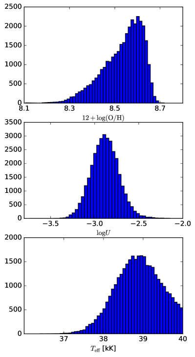
Figure 5: Histograms containing the oxygen abundances (left panel), logarithm of the ionization parameter (middle panel) and effective temperature values (rigth panel) for the sample of objects presented in Section 2.2.

In Fig. 5, we present three histograms containing the oxygen abundances, logarithm of the ionization parameter and $T_{\rm eff}$ values obtained for the objects in our sample applying the methodology described above. We can see that the oxygen abundance values (left panel) are in the range $\rm 8.2\>\la\>12+\log(O/H)\>\la\>8.8$ [equivalent to $0.3\>\la\>(Z/Z_{\odot})\>\la\>1.3$], with most objects presenting 12+log(O/H) around of 8.6 [$(Z/Z_{\odot})\approx 0.8$].

Regarding the distribution of the ionization parameter (Fig. 5, middle panel), it is in the $-3.4\>\la\>\log U\>\la\>-2.5$ range, with an average value of about $-2.8$. Higher values for the ionization parameter than the ones derived by us seem to be most frequently found in objects with low metallicity, such as the $U$ values ($\approx-1.3$ dex) derived by Lagos et al. (2018) for the central parts of the star-forming dwarf galaxies UM 461 and Mrk 600.

Concerning the effective temperature, it can be seen in Fig. 5 (rigth panel) that most of the estimated $T_{\rm eff}$ values are around of 39 kK, with an average value of $38.5\pm 1.0$ kK, being the scatter in the order of the uncertainty of our method, i.e. 2.5 kK (see Paper I). It should be noted that this estimation for the uncertainty is an upper limit of the uncertainty for a single star-forming region, while in this work we use many data points to estimate the distribution of $T_{\rm eff}$. As described above, there is an artificial cut in $T_{\rm eff}$ at 40 kK due to the applied method (see Paper I). Nevertheless, star-forming regions can be ionized by stars with $T_{\rm eff}$ higher than 40 kK. For example, Morisset et al. (2016) and Stasińska & Leitherer (1996) compared results of a grid of photonization models with observational data of star-forming regions. They estimated the slopes of the SEDs of the ionizing sources, defined as the ratio between the number of neutral hydrogen ($\rm H^{0}$) and helium ($\rm He^{0}$) ionizing photons: $Q_{o/1}=Q({\rm H^{0}})/Q(\rm He^{0})$ (a kind of softness parameter). These estimated slopes are in the 0.1-1.0 range, which translates into $T_{\rm eff}$ close to or above 40 kK. It is worth mention that only for few objects the $T_{\rm eff}$ estimated values were higher than 40 kK, i.e. most of the objects present $T_{\rm eff}$ values in the 30-40 kK range. This result is in agreement with recent $T_{\rm eff}$ estimations by Ramírez-Agudelo et al. (2017), who used ground-based optical spectroscopy obtained in the framework of the VLT-FLAMES Tarantula Survey (VFTS) to determine parameters of 72 single O-type stars.

Estimations of $T_{\rm eff}$ and consequently the $T_{\rm eff}$ gradients are dependent on the stellar atmosphere model assumed in the photoionization models (e.g. Stasińska & Schaerer 1997; Dors & Copetti 2003; Morisset et al. 2004; Morisset 2004) and on the match between the metallicity of the atmosphere models and the gas (Morisset, 2004). In our case, the $T_{\rm eff}$-$R$ relation was derived assuming the WM-basic stellar atmosphere models (Pauldrach et al., 2001), which are available only for two metallicities: solar and half solar. Therefore, there is an inconsistent match between the stellar and gas metallicities for the photoionization models with $(Z/Z_{\odot})$=0.03 and 0.2, which does overpredict the $T_{\rm eff}$ value for low metallicity objects, reducing the effective gradient generally found in spiral galaxies (Morisset, 2004; Dors et al., 2011). However, as can be seen in Fig. 5 (middle panel), most of the objects ($\approx 82\%$) present $\rm 12+log(O/H)\>\ga\>8.4$ $[\mathrm{i.e.\ }(Z/Z_{\odot})\>\ga\>0.5]$. Therefore, the missmatch between the stellar and gas metallicities in low metallicity models has little effect on our $T_{\rm eff}$ estimations.

In Fig. 6 we present histograms containing the estimated values for gradients of: $T_{\rm eff}$, $\log U$, and oxygen abundance for our sample of galaxies. We can see that for most of the galaxies ($\sim 70$ %) positive values of $T_{\rm eff}$ gradient are derived, despite of a number of flat and negative gradients. The median value of the $T_{\rm eff}$ radial gradients is 0.762 kK/R₂₅, the minimum and the maximum values are -1.8 and 2.9, respectively. The prevalence of positive $T_{\rm eff}$ gradients is compatible with what is expected under the hypothesis that stars are formed following an Initial Mass Function (IMF) with an universal upper mass limit ($M_{\rm up}$) and the variation of the $T_{\rm eff}$ with the galactocentric distance is due to line blanketing effects taking place in the stellar atmospheres. Alternatively, this prevalence could be due to an increment in the $M_{\rm up}$ of the IMF (and then its $T_{\rm eff}$) as the metallicity decreases.

Dors et al. (2017) analyzed $T_{\rm eff}$ in a small sample of 14 spiral galaxies and also found that most of the galaxies ($\sim 80$ %) presents positive gradients while others show flat ($\sim 15$ %) or negative ($\sim 5$ %) slopes. Similar results were found by Pérez-Montero & Vílchez (2009), who studied the behaviour of the $\eta^{\prime}$ parameter (sensitive to $T_{\rm eff}$) along the disk of 12 galaxies. Therefore, in consonance with Dors et al. (2017) and Pérez-Montero & Vílchez (2009), we found that although positive $T_{\rm eff}$ gradients are present in the disk of most of spiral galaxies, this is not an universal property.

In the middle panel of Fig. 6 we can note that both negative and positive gradients of $\log U$ are derived for our sample of galaxies, with a tendency to derive negative gradients more frequently presenting a median value of -0.1 dex/R₂₅ and being in the range from -0.5 to 0.8  dex/R₂₅. The overwhelming majority of galaxies in our sample have negative oxygen abundance gradients being in the range from -0.43 to 0.04 dex/R₂₅ (see lower panel of the same figure). The median value of the oxygen abundance gradient is -0.15 dex/R₂₅.

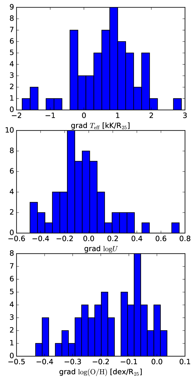
Figure 6: Histograms containing estimated values for the gradients of: $T_{\rm eff}$ (upper panel), $\log U$ middle panel), and $\log(\rm O/H)$ (lower panel) for our sample of galaxies.

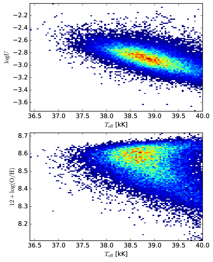
Figure 7: Density maps for the individual spaxels of our sample of CALIFA galaxies. Top panel. $\log U$ as a function of $T_{\rm eff}$. Bottom panel. Oxygen abundance as a function of $T_{\rm eff}$.

To investigate the correlation between $T_{\rm eff}$ and the other studied nebular parameters: $\log U$ and 12+$\log(\rm O/H)$, we plot in Fig. 7 these parameters as a function of $T_{\rm eff}$ for the individual spaxels of our sample. Top panel of this figure shows that $\log U$ decreases as $T_{\rm eff}$ increases. This result is in agreement with the one derived by Morisset et al. (2016), who found that $Q_{0/1}$ (wich is inversely proportional to $T_{\rm eff}$) is increasing with $\log U$. This result indicates that cooler stars lead to higher $U$, in contradiction with the assumption that H ii regions ionized by hotter stars would have higher $U$ because these stars are emitting more ionizing photons. Sanders et al. (2016) showed that the ionization parameter has a weak dependence on both the rate of ionizing photon production and the gas density, and is somewhat more sensitive to the volume filling factor ($\epsilon$):

$$U\>\propto Q({\rm H})^{1/3}\>N_{\rm e}^{1/3}\>\epsilon^{2/3}.$$ (12)

Therefore, it is possibly that nebulae ionized by cooler stars present higher $\epsilon$ (and consequentely higher $U$) than those ionized by hotter stars.

Despite of the conclusions by Shields & Searle (1978); Vilchez & Pagel (1988); Henry & Howard (1995); Dors & Copetti (2003, 2005), who claimed that high metallicity H ii regions have lower $T_{\rm eff}$ compared to those with low metallicity, we do not find any clear correlation between $T_{\rm eff}$ and 12+$\log(\rm O/H)$ for the spaxels of all galaxies in our sample (see also Morisset 2004; Dors et al. 2017). Contradiction between previous and current results can be caused by the fact that the $T_{\rm eff}$ – metallicity relation is not unique, i.e. this relation is different for the different galaxies. This suggestion will be discussed below.

In Fig. 8 we plotted 12+$\log(\rm O/H)$ versus $\log U$ where a large scatter is noted and not apparent correlation can be seen between both parameters. This result is in consonance with, for example, the one found by Dors et al. (2011), who derived oxygen abundances and ionization parameters from diagnostic diagrams containing photoionization model results and observational data of H ii regions. Kaplan et al. (2016) presented a study of the excitation conditions and metallicities in eight nearby spiral galaxies from the VIRUS-P Exploration of Nearby Galaxies (VENGA) survey. These authors calculated the ionization parameter by using an iterative determination proposed by Kewley & Ellison (2008), and they did not notice any clear trends between $U$ and $Z$ (see also Lara-López et al. 2013). In other hand, a trend for H ii regions showing that those with higher values of $\log U$ present lower metallicities was derived, for example, by Morisset et al. (2016), who used a large grid of photoionzation models in order to reproduce emission line intensities also taken from the CALIFA database (see also Pérez-Montero & Amorín 2017 and references therein). The relation between ionization paremeter and oxygen abundance seems to be dependent on the methodology employed to calculate these parameters (e.g. Krühler et al. 2017) or on the geometry assumed in the photoionization models (see, for example, Fig. 13 of Morisset et al. 2016.)

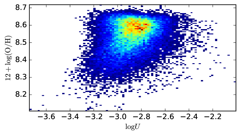
Figure 8: Same as Fig. 7 for 12+$\log(\rm O/H)$ as a function of $\log U$.

Fig. 9 shows the central $T_{\rm eff}$, gradients of $T_{\rm eff}$ and $\log U$, and 12+$\log(\rm O/H)_{0}$ as a function of the stellar mass of the galaxies. Central $T_{\rm eff}$ was calculated as the average values for the spaxels with $R<0.2R_{25}$. We found no correlation between central $T_{\rm eff}$, $T_{\rm eff}$ and $\log U$ gradients and the stellar mass of the galaxies.

The radial gradients of $\log U$ and $T_{\rm eff}$ as a function of oxygen abundance gradient are shown in Fig. 10, finding a correlation in both cases. The former presents a positive correlation, the gradient of $\log U$ increases as the $\log(\rm O/H)$ gradient increases. As the p-value is 0.0001, null hypothesis that there is no correlation between $\log U$ and ${\rm O/H}$ should be rejected. On the other hand, an anti-correlation between the gradient of $T_{\rm eff}$ and the oxygen abundance gradient is clearly seen for our sample with a p-value of $10^{-5}$. Moreover, galaxies with flat oxygen abundance gradients tend to have flat $\log U$ and $T_{\rm eff}$ gradients too. Therefore, one can expect an anti-correlation between the $T_{\rm eff}$ and the oxygen abundance. Indeed, such anti-correlation can be seen in the low metallicity zone on the bottom panel of Fig. 7. However, at the high metallicity regime there is no correlation between $T_{\rm eff}$ and $\log(\rm O/H)$ for individual spaxels. Using the softness parameter defined by Vilchez & Pagel (1988) as

$$\eta^{\prime}\,=\,\frac{([\textrm{O\,{\sc ii}}]\lambda\lambda 3727,3729/[\textrm{O\,{\sc iii}}]\lambda\lambda 4959,5007)}{([\textrm{S\,{\sc ii}}]\lambda\lambda 6717,6731/[\textrm{S\,{\sc iii}}]\lambda\lambda 9069,9532)},$$

which works as a diagnostic for the nature and the efective temperature of the ionizing radiation field (see Díaz et al., 1985), Díaz et al. (2007) and Hägele (2008) compared the ionization structure for star-forming regions in different environments. They found that high metallicity Circumnuclear Star Forming Regions (CNSFRs) segregates from high metallicity disk H ii regions, with the former showing $T_{\rm eff}$ values of about 40 kK and the last ones of about 35 kK, a temperature range similar to those found by us for the objects in the high metallicity regime. On the other hand, these authors also found that the low metallicity H ii galaxies belonging to their sample (see also the H ii galaxies studies by Hägele et al., 2006, 2008, 2011, 2012; Pérez-Montero et al., 2010) present a similar behaviour and $T_{\rm eff}$ values (40 kK) than those shown by the CNSFRs. In all the cases the low metallicity H ii galaxies show high $T_{\rm eff}$ values, in agreement with the results derived from Fig. 7. A possible explanation of this fact could be that, for an individual galaxy, the $T_{\rm eff}$ increases as the oxygen abundance decreases but there is not a unique $T_{\rm eff}$ – $\log(\rm O/H)$ relation for all galaxies.

Finally, the averaged $T_{\rm eff}$ for the spaxels with $R\><\>0.2R_{25}$ ($T_{\rm eff,0}$) as a function of the $T_{\rm eff}$ value extrapolated to $R=0.1R_{25}$ ($T_{\rm eff,center}$) is plotted in the upper panel of Fig. 11. It shows that for the galaxies in our sample the $T_{\rm eff,0}$ can be significantly lower than the $T_{\rm eff,center}$. This fact could be considered as an indication that the star formation processes at the central parts of galaxies, which determine the $T_{\rm eff}$, are not similar to those along the disks. This could be due to metallicity effects, in the sense that metallicities at the center could be higher than the ones expected extrapolating the radial O/H gradient, which leads to the cooling of the atmospheres of massive stars. However, the behaviour of the $\rm(O/H)_{0}$ versus $\rm(O/H)_{center}$ for the galaxies in our sample (bottom panel of Fig. 11) does not show significant bias between $\rm(O/H)_{0}$ and $\rm(O/H)_{center}$. Thus, another effect rather than metallicity seems to be responsible for producing the discrepancy between $T_{\rm eff,0}$ and $T_{\rm eff,center}$, since not only the metallicity controls the $T_{\rm eff}$. Star formation processes in nuclear regions of galaxies can be altered by, for example, supernova explosions and/or the presence of Wolf Rayet stars (most common in high metallicity environments). Moreover, the gas outflows found in nuclear starbursts and in Active Galaxy Nuclei, that extends on kiloparsec scales, could potentially suppress star formation in their host galaxies (Gallagher et al., 2018) modifying the $T_{\rm eff}$ expected from the radial gradient and producing the discrepancy seen in Fig. 11. Also, gas flux from outskirts parts of the disks (e.g. Rosa et al. 2014) could be falling into the nucleus modifying the star formation processes.

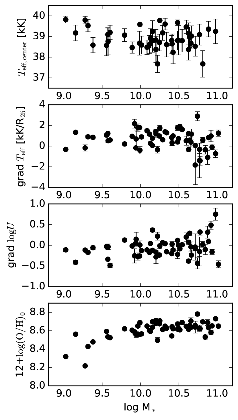
Figure 9: Panels from top to bottom: central $T_{\rm eff}$ (average values), radial gradients of $T_{\rm eff}$, radial gradients of $\log U$, and 12+$\log(O/H)_{0}$ as a function of the stellar mass of the galaxy.

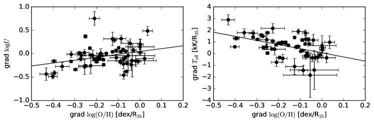
Figure 10: Left panel: Radial gradient of $\log U$ as a function of the oxygen abundance radial gradient. Right panel: Radial gradient of $T_{\rm eff}$ as a function of the oxygen abundance radial gradient. Solid lines are the best fit linear regression to the data.

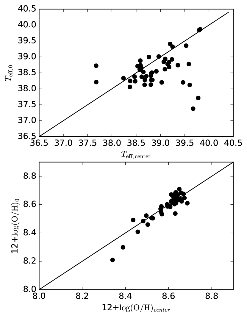
Figure 11: Upper panel: Comparison of $T_{\rm eff,0}$ and $T_{\rm eff,center}$. Bottom panel: Relation between 12+log(O/H)₀ and 12+log(O/H)_center. In both panels the one-to-one relation is shown.

4 Conclusion

We used homogeneous spectroscopic data of H ii regions taken from the CALIFA survey and a theoretical calibration between the effective temperature of ionizing star(s) ($T_{\rm eff}$) and the ratio $R$ = $\log$([O ii]$\lambda\lambda$3727,3729/[O iii]$\lambda$5007) to investigate the universality of $T_{\rm eff}$ gradients in spiral galaxies as well as correlation between $T_{\rm eff}$, the ionization parameter ($U$) and the oxygen abundance of H ii regions. We found that most of the galaxies in our sample ($\sim 70$ %) presents positive $T_{\rm eff}$ radial gradients, with a median value of 0.762 kK/$R_{25}$, even though some galaxies exhibit negative or flat $T_{\rm eff}$ radial gradients. Therefore, we conclude that $T_{\rm eff}$ gradients are not an universal property of spiral galaxies. We also found that radial gradients of both $\log U$ and $T_{\rm eff}$ depend on the oxygen abundance gradient, in the sense that the gradient of $\log U$ increases as the $\log({\rm O/H})$ gradient increases while the $T_{\rm eff}$ gradient decreases as the $\log({rmO/H})$ increases. Moreover, galaxies with flat oxygen abundance gradient tend to have flat $\log U$ and $T_{\rm eff}$ gradients.

References

- Abbott & Hummer (1985) Abbott D. C., Hummer D. G., 1985, ApJ, 294, 286
- Allende Prieto et al. (2001) Allende Prieto C., Lambert D. L., Asplund M., 2001, ApJ, 556, L63
- Asari et al. (2007) Asari N. V., Cid Fernandes R., Stasińska G., Torres-Papaqui J. P., Mateus A., Sodré L., Schoenell W., Gomes J. M., 2007, MNRAS, 381, 263
- Baldwin et al. (1981) Baldwin J. A., Phillips M. M., Terlevich R., 1981, PASP, 93, 5
- Bastian et al. (2010) Bastian N., Covey K. R., Meyer M. R., 2010, ARA&A, 48, 339
- Bruzual & Charlot (2003) Bruzual G., Charlot S., 2003, MNRAS, 344, 1000
- Cardelli et al. (1989) Cardelli J. A., Clayton G. C., Mathis J. S., 1989, ApJ, 345, 245
- Cid Fernandes et al. (2005) Cid Fernandes R., Mateus A., Sodré L., Stasińska G., Gomes J. M., 2005, MNRAS, 358, 363
- Corti et al. (2007) Corti M., Bosch G., Niemela V., 2007, A&A, 467, 137
- Crowther et al. (2016) Crowther P. A., et al., 2016, MNRAS, 458, 624
- Díaz et al. (1985) Díaz A. I., Pagel B. E. J., Wilson I. R. G., 1985, MNRAS, 212, 737
- Díaz et al. (2007) Díaz A. I., Terlevich E., Castellanos M., et al. 2007, MNRAS, 382, 251
- Dors & Copetti (2003) Dors Jr. O. L., Copetti M. V. F., 2003, A&A, 404, 969
- Dors & Copetti (2005) Dors Jr. O. L., Copetti M. V. F., 2005, A&A, 437, 837
- Dors et al. (2011) Dors Jr. O. L., Krabbe A., Hägele G. F., Pérez-Montero E., 2011, MNRAS, 415, 3616
- Dors et al. (2017) Dors O. L., Hägele G. F., Cardaci M. V., Krabbe A. C., 2017, MNRAS, 466, 726
- Ellison et al. (2008) Ellison S. L., Patton D. R., Simard L., McConnachie A. W., 2008, ApJ, 672, L107
- Ellison et al. (2018) Ellison S. L., Sánchez S. F., Ibarra-Medel H., Antonio B., Mendel J. T., Barrera-Ballesteros J., 2018, MNRAS, 474, 2039
- Evans (1986) Evans I. N., 1986, ApJ, 309, 544
- Evans et al. (2015) Evans C. J., et al., 2015, A&A, 574, A13
- Fierro et al. (1986) Fierro J., Torres-Peimbert S., Peimbert M., 1986, PASP, 98, 1032
- Gallagher et al. (2018) Gallagher R., Maiolino R., Belfiore F., Drory N., Riffel R., Riffel R. A., 2018, preprint, (arXiv:1806.03311)
- Hägele (2008) Hägele G. F., 2008, PhD thesis, Universidad Autónoma de Madrid
- Hägele et al. (2006) Hägele G. F., Pérez-Montero E., Díaz A. I., et al. 2006, MNRAS, 372, 293
- Hägele et al. (2008) Hägele G. F., Díaz A. I., Terlevich E., et al. 2008, MNRAS, 383, 209
- Hägele et al. (2011) Hägele G. F., García-Benito R., Pérez-Montero E., et al. 2011, MNRAS, 414, 272
- Hägele et al. (2012) Hägele G. F., Firpo V., Bosch G., et al. 2012, MNRAS, 422, 3475
- Henry & Howard (1995) Henry R. B. C., Howard J. W., 1995, ApJ, 438, 170
- Holgado et al. (2018) Holgado G., et al., 2018, A&A, 613, A65
- Husemann et al. (2013) Husemann B., Wisotzki L., Sánchez S. F., Jahnke K., 2013, A&A, 549, A43
- Izotov et al. (1994) Izotov Y. I., Thuan T. X., Lipovetsky V. A., 1994, ApJ, 435, 647
- Kaplan et al. (2016) Kaplan K. F., et al., 2016, MNRAS, 462, 1642
- Kennicutt et al. (2000) Kennicutt Jr. R. C., Bresolin F., French H., Martin P., 2000, ApJ, 537, 589
- Kewley & Ellison (2008) Kewley L. J., Ellison S. L., 2008, ApJ, 681, 1183
- Kewley et al. (2001) Kewley L. J., Dopita M. A., Sutherland R. S., Heisler C. A., Trevena J., 2001, ApJ, 556, 121
- Kinman & Davidson (1981) Kinman T. D., Davidson K., 1981, ApJ, 243, 127
- Krühler et al. (2017) Krühler T., Kuncarayakti H., Schady P., Anderson J. P., Galbany L., Gensior J., 2017, A&A, 602, A85
- Lagos et al. (2018) Lagos P., Scott T. C., Nigoche-Netro A., Demarco R., Humphrey A., Papaderos P., 2018, MNRAS, 477, 392
- Lamb et al. (2016) Lamb J. B., Oey M. S., Segura-Cox D. M., Graus A. S., Kiminki D. C., Golden-Marx J. B., Parker J. W., 2016, ApJ, 817, 113
- Lara-López et al. (2010) Lara-López M. A., et al., 2010, A&A, 521, L53
- Lara-López et al. (2013) Lara-López M. A., López-Sánchez Á. R., Hopkins A. M., 2013, ApJ, 764, 178
- Lequeux et al. (1979) Lequeux J., Peimbert M., Rayo J. F., Serrano A., Torres-Peimbert S., 1979, A&A, 80, 155
- Mannucci et al. (2010) Mannucci F., Cresci G., Maiolino R., Marconi A., Gnerucci A., 2010, MNRAS, 408, 2115
- Markova et al. (2018) Markova N., Puls J., Langer N., 2018, A&A, 613, A12
- Martins & Palacios (2017) Martins F., Palacios A., 2017, A&A, 598, A56
- Martins et al. (2004) Martins F., Schaerer D., Hillier D. J., Heydari-Malayeri M., 2004, A&A, 420, 1087
- Martins et al. (2005) Martins F., Schaerer D., Hillier D. J., 2005, A&A, 436, 1049
- Massey et al. (2005) Massey P., Puls J., Pauldrach A. W. A., Bresolin F., Kudritzki R. P., Simon T., 2005, ApJ, 627, 477
- Massey et al. (2009) Massey P., Zangari A. M., Morrell N. I., Puls J., DeGioia-Eastwood K., Bresolin F., Kudritzki R.-P., 2009, ApJ, 692, 618
- Mateus et al. (2006) Mateus A., Sodré L., Cid Fernandes R., Stasińska G., Schoenell W., Gomes J. M., 2006, MNRAS, 370, 721
- Mohr-Smith et al. (2017) Mohr-Smith M., et al., 2017, MNRAS, 465, 1807
- Mokiem et al. (2004) Mokiem M. R., Martín-Hernández N. L., Lenorzer A., de Koter A., Tielens A. G. G. M., 2004, A&A, 419, 319
- Morisset (2004) Morisset C., 2004, ApJ, 601, 858
- Morisset et al. (2004) Morisset C., Schaerer D., Bouret J.-C., Martins F., 2004, A&A, 415, 577
- Morisset et al. (2016) Morisset C., et al., 2016, A&A, 594, A37
- Morrell et al. (2014) Morrell N. I., Massey P., Neugent K. F., Penny L. R., Gies D. R., 2014, ApJ, 789, 139
- Pauldrach et al. (2001) Pauldrach A. W. A., Hoffmann T. L., Lennon M., 2001, A&A, 375, 161
- Peimbert & Serrano (1982) Peimbert M., Serrano A., 1982, MNRAS, 198, 563
- Pérez-Montero & Amorín (2017) Pérez-Montero E., Amorín R., 2017, MNRAS, 467, 1287
- Pérez-Montero & Vílchez (2009) Pérez-Montero E., Vílchez J. M., 2009, MNRAS, 400, 1721
- Pérez-Montero et al. (2010) Pérez-Montero E., García-Benito R., Hägele G. F., Díaz Á. I., 2010, MNRAS, 404, 2037
- Pilyugin & Grebel (2016) Pilyugin L. S., Grebel E. K., 2016, MNRAS, 457, 3678
- Pilyugin et al. (2004) Pilyugin L. S., Vílchez J. M., Contini T., 2004, A&A, 425, 849
- Ramírez-Agudelo et al. (2017) Ramírez-Agudelo O. H., et al., 2017, A&A, 600, A81
- Rosa et al. (2014) Rosa D. A., Dors O. L., Krabbe A. C., Hägele G. F., Cardaci M. V., Pastoriza M. G., Rodrigues I., Winge C., 2014, MNRAS, 444, 2005
- Rubin et al. (1984) Rubin V. C., Ford Jr. W. K., Whitmore B. C., 1984, ApJ, 281, L21
- Sánchez et al. (2012) Sánchez S. F., et al., 2012, A&A, 538, A8
- Sánchez et al. (2013) Sánchez S. F., et al., 2013, A&A, 554, A58
- Sánchez et al. (2016) Sánchez S. F., et al., 2016, A&A, 594, A36
- Sánchez et al. (2017) Sánchez S. F., et al., 2017, MNRAS, 469, 2121
- Sanders et al. (2016) Sanders R. L., et al., 2016, ApJ, 816, 23
- Schaerer & Schmutz (1994) Schaerer D., Schmutz W., 1994, A&A, 288, 231
- Shields & Searle (1978) Shields G. A., Searle L., 1978, ApJ, 222, 821
- Simón-Díaz et al. (2014) Simón-Díaz S., Herrero A., Sabín-Sanjulián C., Najarro F., Garcia M., Puls J., Castro N., Evans C. J., 2014, A&A, 570, L6
- Skillman (1992) Skillman E. D., 1992, in Edmunds M. G., Terlevich R., eds, Elements and the Cosmos. p. 246
- Sota et al. (2011) Sota A., Maíz Apellániz J., Walborn N. R., Alfaro E. J., Barbá R. H., Morrell N. I., Gamen R. C., Arias J. I., 2011, ApJS, 193, 24
- Stasińska & Leitherer (1996) Stasińska G., Leitherer C., 1996, ApJS, 107, 661
- Stasińska & Schaerer (1997) Stasińska G., Schaerer D., 1997, A&A, 322, 615
- Storey & Zeippen (2000) Storey P. J., Zeippen C. J., 2000, MNRAS, 312, 813
- Tramper et al. (2014) Tramper F., Sana H., de Koter A., Kaper L., Ramírez-Agudelo O. H., 2014, A&A, 572, A36
- Tremonti et al. (2004) Tremonti C. A., et al., 2004, ApJ, 613, 898
- Vilchez & Pagel (1988) Vilchez J. M., Pagel B. E. J., 1988, MNRAS, 231, 257
- Walborn et al. (2014) Walborn N. R., et al., 2014, A&A, 564, A40
- Walcher et al. (2014) Walcher C. J., et al., 2014, A&A, 569, A1
- Wright (2006) Wright E. L., 2006, PASP, 118, 1711
- Wright et al. (2015) Wright N. J., Drew J. E., Mohr-Smith M., 2015, MNRAS, 449, 741
- Zanstra (1929) Zanstra H., 1929, Publications of the Dominion Astrophysical Observatory Victoria, 4
- Zinchenko et al. (2016) Zinchenko I. A., Pilyugin L. S., Grebel E. K., Sánchez S. F., Vílchez J. M., 2016, MNRAS, 462, 2715
- Zinchenko et al. (2018) Zinchenko I. A., Just A., Pilyugin L. S., Lara-Lopez M. A., 2018, preprint, (arXiv:1810.08006)