A new class of curves generalizing helix and rectifying curves

Abstract

In this paper, we introduce a new class of curves $\alpha$ called a $f$-rectifying curves, which its $f$-position vector defined by $\alpha_{f}(s)=\int f(s)T(s)ds$ always lie in the rectifying plane of $\alpha$, where $f$ is an integrable function and $T$ is the speed curve of $\alpha$. In particular case, when the function $f\equiv 0$ or constant, the class of $f$-rectifying curves are helix or rectifying curves, respectively. The classification and the characterization of such curves in terms of their curvature and the torsion functions are given with a physical interpretation. We close this study with some examples.

Key words: $f$-rectifying; $f$-position vector; helix; rectifying.

AMS Subject Classification: 53A04, 53A17

1 Introduction

Let $\mathbb{E}^{3}$ be an Euclidean 3-space, we denote by $<x,y>$ the standard inner product for any arbitrary vectors $x$ and $y$ in $\mathbb{E}^{3}$. The norm of $x$ is denoted by $\left|x\right|=\sqrt{<x,x>}$.

Let $\alpha:I\subset\mathbb{R}\rightarrow\mathbb{E}^{3}$ be a non null speed curve. The arc-length parameter $s$ of a curve $\alpha$ is determined such that $\left|\alpha^{\prime}(s)\right|=\left|T(s)\right|=1$. We define the curvature function of $\alpha$ by $\kappa(s)=\left|T^{\prime}(s)\right|.$ If $\kappa(s)\neq 0,$ then the unit principal normal vector $N(s)$ of the curve $\alpha$ at $s$ is given by $\alpha^{\prime\prime}(s)=T^{\prime}(s)=\kappa(s)N(s).$ The binormal vector is $B(s)=T(s)\times N(s)$ (the symbol $\times$ is vector product).

The Frenet-Serret formulas are

$$T^{\prime}=\kappa N;\ \ N^{\prime}=-\kappa T+\tau B;\ \ B^{\prime}=-\tau N$$ (1)

where the function $\tau(s)$ is the torsion function of $\alpha$ at $s$. A curve is called a twisted curve if has non zero curvature and torsion. The planes spanned by $\{T,N\}$, $\{T,B\}$, and $\{N,B\}$ are called the osculating plane, the rectifying plane, and the normal plane, respectively.

We keep the name helix for a curve $\alpha$ in $\mathbb{E}^{3}$ if its tangent vector $T$ makes a constant angle with a fixed direction $X$ called also the axis. The vector $X$ along helix curve lies in the rectifying plane, it can be given by

$$X=\cos\theta\ T+\sin\theta\ B$$ (2)

here $\theta$ is a constant angle different from $\frac{\pi}{2}$ (see [3]).
In [4], the author introduce a rectifying curves, as space curves $\alpha$ whose position vector always lie in its rectifying plane. The position vector $\alpha(s)$ of a rectifying curve satisfies

$$\alpha(s)=(s+a)T+bB$$ (3)

where $a$ and $b$ are some real constants.
In the terms of curvature and torsion, a curve $\alpha$ is a general helix and congruent to a rectifying curve if and only if the ratio of torsion to curvature is

$$\frac{\tau}{\kappa}=c_{1}\text{ (constant)}$$ (4)

and

$$\frac{\tau}{\kappa}=c_{2}s+c_{3}\text{ (linear function)},$$ (5)

respectively, where $c_{1,2}$ is non null constants and $c_{3}$ is a constant.
Therefore, the rectifying plane of a curve $\alpha$ play an important role to this two classes of curves (i.e. helix and rectifying).

Motivated by above definitions of helix and rectifying curves given in Eq.(2 and 3), and their characterizations in the terms of curvature and torsion given in Eq.(4 and 5), it is natural to ask the following geometric question: Is there a class of curves generalizing the classes of helix and rectifying curves?

Firstly, let’s define a new vector $\alpha_{f}$ that we call’it $f$-position vector of the curve $\alpha$ by

$$\alpha_{f}(s)=\int f(s)T(s)ds$$

where $f$ is an integrable function. By a simple calculate, for $f\equiv 0$ we find the right side of Eq.(2) and for non null constant function $f,$ we get, up to parametrization, right side of the Eq.(3).
When the $f$-position vector $\alpha_{f}$ lie in the rectifying plane of $\alpha$ i.e.

$$\alpha_{f}(s)=\int f(s)T(s)ds=\lambda(s)T+\mu(s)B$$ (6)

for $f(s)\equiv 0$ and $f(s)\equiv f$ (constant), we find helix and rectifying definitions, respectively, where $\lambda$ and $\mu$ are some functions. The generalization in the terms of curvature and the torsion functions of the Eqs(4 and 5) will be presented in the Theorem 3.

Now, we are able to introduce the following definition about such curves.

Definition 1

Let $\alpha:I\subset\mathbb{R}\rightarrow\mathbb{E}^{3}$ be a curve with Frenet apparatus $\{T,N,B,\kappa,\tau\}$ and $f$ be an integrable function in parameter $s.$ We call the curve $\alpha$ a $f$-rectifying curve if its $f$-position vector $\alpha_{f}$ lie always in the rectifying plane of $\alpha$ i.e.

$$\alpha_{f}(s)=\lambda(s)T+\mu(s)B$$

where $\lambda(s)$ and $\mu(s)$ are some real functions.

Consequently, the Definition 1 coincides with helix curve or rectifying curve definitions when the function $f$ is a null or a constant, respectively.
Hence, when the function $f$ varies in the set of all integrable functions, the $f$-position vector $\alpha_{f}$ give an enlarged determination of $\alpha$ and the class of $f$-rectifying curves present a generalization of helix and rectifying space curves.

The paper is organized as follow;
In the section 2, we give characterizations of $f$-rectifying curves by the Theorem 2. In section 3, we prove that a twisted curve is congruent to a $f$-rectifying curve if and only if the ratio $\tau/\kappa$ is the primitive function $F$ of $f.$ We also give a physical signification of $f$-rectifying curves in mechanics terms. The end section is devoted to the determination explicitly of all $f$-rectifying curves and we close this study with some examples.

2 Characterization of $f$-rectifying curves

For the characterizations of $f$-rectifying curves, we have the following theorem

Theorem 2

Let $\alpha:I\subset\mathbb{R}\rightarrow\mathbb{E}^{3}$ be a $f$-rectifying ($f$ is nonzero function) curve with strictly positive curvature function and $s$ be its arclength. Then
1. The norm function $\rho(s)=\left|\alpha_{f}(s)\right|$ satisfies

$$\rho(s)=\sqrt{F^{2}(s)+c^{2}}$$

where $F$ is the primitive function of $f$ and $c$ is a non null constant.
2. The tangential component of the $f$-position vector $\alpha_{f}$ is

$$\left\langle\alpha_{f},T\right\rangle=F(s)$$

3. The normal component of the $f$-position vector $\alpha_{f}$ has constant length.
4. The torsion $\tau$ is nonzero, and the binormal component of the $f$-position vector $<\alpha_{f},B>$ is constant.
Conversely, if $\alpha:I\subset\mathbb{R}\rightarrow\mathbb{E}^{3}$ is a curve with a positive curvature $\kappa$ and if one of the assertions 1, 2, 3 or 4 holds, then $\alpha$ is a $f$-rectifying curve.

Proof. Let $\alpha:I\subset\mathbb{R}\rightarrow\mathbb{E}^{3}$ be a $f$-rectifying curve parameterized by arclength $s,$ we suppose that $\alpha$ is non helix curve (i.e. $f$ nonzero function). From the Definition 1, we have

$$\alpha_{f}(s)=\int f(s)d\alpha=\lambda(s)\ T+\mu(s)\ B$$

Differentiating the Eq.(6) with respect to $s$ and using the Frenet formulas Eq.(1), we get

$$f(s)T=\lambda^{\prime}(s)\ T+\left(\lambda(s)\kappa-\mu(s)\tau\right)N+\mu^{\prime}(s)\ B$$

by comparing, we have

$$\left\{\begin{array}[]{l}\lambda(s)=\int f(s)ds=F(s)\\ \dfrac{\tau}{\kappa}=\dfrac{\lambda(s)}{\mu(s)},\\ \mu(s)=\mu\text{ non null constant}\end{array}\right.$$ (7)

1. We have for the norm function

$$\rho^{2\prime}(s) = 2\left\langle\alpha_{f}(s),f(s)T\right\rangle=2\left\langle F(s)T+\mu B,f(s)T\right\rangle$$

$$= 2F(s)f(s)=F^{2^{\prime}}(s)\ \text{and}$$

$$\rho^{2}(s) = F^{2}(s)+\bar{c}$$ (9)

Because $0$ is in $I$, we must have $\bar{c}>0$, then

$$\rho(s)=\sqrt{F^{2}(s)+c^{2}}$$

where $\bar{c}=c^{2}$.
2. It’s a direct consequence from the equations Eq.(6) and Eq.(7)₍₁₎.
3. Let us put $\alpha_{f}(s)=m(s)T(s)+\alpha_{f}^{N}(s)$, where $m(s)$ is arbitrary differentiable function. Comparing with the Eq. (6), we conclude that $\alpha_{f}^{N}(s)=\mu B,$ and $\left\langle\alpha_{f}^{N}(s),B\right\rangle=\mu$ is a constant from Eq.(7)₍₃₎ then this yields assertion (3).
4. We can easily get (4) from Eq.(7)_(1,2) and the fact that $\kappa>0$.
Conversely,
Suppose that the assertions (1) or (2) holds. Then we have $\left\langle\alpha_{f}(s),T\right\rangle=F(s)$ and by taking the derivative of the last equation with respect to $s$, we get $\kappa\left\langle\alpha_{f}(s),N\right\rangle=0$. Taking account that $\kappa>0$, we have $\left\langle\alpha_{f},N\right\rangle=0,$ i.e $\alpha$ is $f$-rectifying curve.
If the assertion (3) holds, from the Eq.(2), we have

$$\left\langle\alpha_{f}(s),\alpha_{f}(s)\right\rangle=\left\langle\alpha_{f},T\right\rangle^{2}+c^{2}$$

by differentiating the last equation with respect to $s$ gives

$$2\left\langle\alpha_{f}(s),f(s)T\right\rangle = 2\left\langle\alpha_{f},T\right\rangle\left(\left\langle f(s)T,T\right\rangle+\kappa\left\langle\alpha_{f}(s),N\right\rangle\right)$$

$$\left\langle\alpha_{f}(s),f(s)T\right\rangle = \left\langle\alpha_{f}(s),f(s)T\right\rangle\left(1+\frac{\kappa}{f(s)}\left\langle\alpha_{f}(s),N\right\rangle\right)$$

Since $\kappa>0,$ $f(s)\neq 0$ and the norm function $\left|\alpha_{f}(s)\right|$ is non constant function then $\left\langle\alpha_{f}(s),N\right\rangle=0$ i.e $\alpha$ is $f$-rectifying curve.
For assertion $(4)$, using the Eq.(1), we can easily get the result.    

3 Helix, rectifying curves compared to the $f$-rectifying curves

From [3] and [4], any twisted curve $\alpha$ is helix if and only if the ratio $\frac{\tau}{\kappa}$ is a nonzero constant, and it is congruent to a rectifying curve if and only if the ratio $\left(\frac{\tau}{\kappa}\right)^{\prime}$ is a non null constant. How about the $f$-rectifying curve case?

The characterization in the terms of the ratio $\frac{\tau}{\kappa}$ is given in the following theorem.

Theorem 3

Let $\alpha:I\subset\mathbb{R}\rightarrow\mathbb{E}^{3}$ be a curve with strictly positive curvature $\kappa$. The curve $\alpha$ is congruent to a $f$-rectifying curve if and only if the ratio of torsion and curvature of the curve is

$$\frac{\tau}{\kappa}=\overline{\mu}F(s)$$

where $F$ is the primitive of $f$ and $\overline{\mu}$ is non null constant.
Moreover, if
i. $f\equiv 0,$ we have the helix condition for $\alpha$, i.e. $\frac{\tau}{\kappa}$ is non null constant,
ii. $f$ is a non null constant function, $\alpha$ is congruent to a rectifying curve, i.e. $\left(\frac{\tau}{\kappa}\right)^{\prime}$ is non null constant,
iii. $f$ is a $n$-degree polynomial, then $\alpha$ has a characterization $\left(\frac{\tau}{\kappa}\right)^{(n+1)}$ is non null constant.

Proof. Let $\alpha:I\subset\mathbb{R}\rightarrow\mathbb{E}^{3}$ be a curve with strictly positive curvature $\kappa.$
If $\alpha$ is $f$-rectifying curve and using The Eq.(7) then

$$\frac{\tau}{\kappa}=\frac{\lambda(s)}{\mu}=\frac{1}{\mu}F(s)=\overline{\mu}F(s)$$

Hence, the ratio of torsion and curvature of the curve $\alpha$ satisfied the assertions $(i)$, $(ii)$ and $(iii)$ according to the values of the function $f$.
Conversely, $\alpha:I\subset\mathbb{R}\rightarrow\mathbb{E}^{3}$ be a curve with positive curvature $\kappa$ such that

$$\frac{\tau}{\kappa}=\overline{\mu}F(s)$$

by using the Frenet-Serret equations given in Eq.(1), we get

$$\frac{d}{ds}(\int f(s)d\alpha-F(s)\ T-\frac{1}{\overline{\mu}}\ B)=0$$

which conclude that $\alpha$ is congruent to a $f$-rectifying curve.    

3.1 Physical interpretation

In mechanics terms and from [4], up to rigid motions, the general helix and the rectifying curves are characterized as those curves that are in equilibrium under the action of the force field

$$\mathbf{F}=f(s)T-\tau N$$

for $f(s)=0$ and nonzero constant $f(s)=f,$ respectively.
If $f(s)$ is non constant function and using the Theorem 3, the curve is not rectifying curve.

In the case when $f$ is non constant function, the $f$-rectifying curves are characterized as those curves that are in equilibrium under the action of the force field $\mathbf{F}$ for non rigid motions.

Now, up to rigid motions, for the action of the force field $\mathbf{\bar{F}}=-\frac{\tau}{F}N$ where $F$ is the primitive function of $f$, here the curve is in equilibrium when it is $f$-rectifying curve. ( For more detail for equilibrium curves definition, see [2] and [1])

4 Classification of $f$-rectifying curves

We determine in the following theorem explicitly all $f$-rectifying curves where $f$ is non null function by dilating a vector $Y$ in $\mathbb{S}^{2}$, with a distance function $\rho.$

Theorem 4

Let $\alpha:I\subset\mathbb{R}\rightarrow\mathbb{E}^{3}$ be a curve with $\kappa>0$ and $f$ be an integrable non null function. Then $\alpha$ is a $f$-rectifying curve if and only if, up to parametrization, it is given by

$$\alpha(t)=\tfrac{c\sec(t+t_{0})}{f(F^{-1}(c\tan(t+t_{0})))}Y(t)-c^{2}\int f^{{}^{\prime}}(F^{-1}(c\tan(t+t_{0})))\left(\tfrac{\sec(t+t_{0})}{f(F^{-1}(c\tan(t+t_{0})))}\right)^{3}Y(t)dt$$ (10)

where $c$ is a strictly positive number, $F$ a primitive function of $f$ with $F(0)=c\tan t_{0},$ and $Y(t)$ is a curve in $\mathbb{S}^{2}$ and not an arc of the great circle.

Proof. Let $\alpha:I\subset\mathbb{R}\rightarrow\mathbb{E}^{3}$ be a $f$-rectifying, without loss of generality, we suppose that $\alpha$ is a unit speed curve with $\kappa>0$ and let us define a unit vector by

$$Y(s)=\frac{\alpha_{f}(s)}{\rho(s)}$$ (11)

Using the Theorem 2 (1), we have

$$\alpha_{f}(s)=\int f(s)d\alpha=\int f(s)T(s)ds=\sqrt{F^{2}(s)+c^{2}}Y(s)$$ (12)

by derivating the Eq.(12) with respect to $s$ and taking account that $Y(s)$ is orthogonal to $Y^{\prime}(s)$, we get

$$f(s)T(s)=\frac{f(s)F(s)}{\sqrt{F^{2}(s)+c^{2}}}Y(s)+\sqrt{F^{2}(s)+c^{2}}Y^{\prime}(s)$$

and

$$f^{2}(s)=\frac{f^{2}(s)F^{2}(s)}{F^{2}(s)+c^{2}}+\left(F^{2}(s)+c^{2}\right)r^{2}$$ (13)

where $r$ denote the norm of $Y^{\prime}$, we suppose that $c$ and $f(s)$ have a similar sign, then the Eq.(13) turns to

$$r=\frac{cf(s)}{F^{2}(s)+c^{2}}$$ (14)

Let us put

$$t=\int_{0}^{s}\frac{cf(u)}{F^{2}(u)+c^{2}}du=\arctan\left(\frac{F(s)}{c}\right)-\arctan\left(\frac{F(0)}{c}\right)$$

then

$$s=F^{-1}(c\tan(t+t_{0}))$$ (15)

where $t_{0}=\arctan\left(\frac{F(0)}{c}\right).$
Substituting the Eq.(15) in the Eq.(12), we have

$$\alpha_{f}(t)=c\sec(t+t_{0})Y(t)$$ (16)

and

$$f(F^{-1}\left(c\tan(t+t_{0})\right))T(t)=c\left(\sec(t+t_{0})\ Y(t)\right)_{t}^{\prime}$$ (17)

by integration by parts, we get finally

$$\alpha(t) = c\int\tfrac{\left(\sec(t+t_{0})\ Y(t)\right)^{\prime}}{f(F^{-1}(c\tan(t+t_{0})))}dt$$

$$= \tfrac{c\sec(t+t_{0})}{f(F^{-1}(c\tan(t+t_{0})))}Y(t)-c\int\left(\left[f(F^{-1}(c\tan(t+t_{0})))\right]^{-1}\right)^{\prime}\sec(t+t_{0})\ Y(t)dt$$

$$= \tfrac{c\sec(t+t_{0})}{f(F^{-1}(c\tan(t+t_{0})))}Y(t)-c^{2}\int f^{{}^{\prime}}(F^{-1}(c\tan(t+t_{0})))\left(\tfrac{\sec(t+t_{0})}{f(F^{-1}(c\tan(t+t_{0})))}\right)^{3}Y(t)dt$$

Now, let calculate the curvature function $\kappa$ of $\alpha.$
The frame $\left\{Y,Y^{\prime},Y\times Y^{\prime}\right\}$ are an orthonormal frame in $\mathbb{E}^{3}$ of unit speed curve $Y(t)$. We have Frenet formulas

$$\left\{\begin{array}[]{ccccc}Y^{\prime}&=&&Y^{\prime}&\\ Y^{\prime\prime}&=&-Y&+&g(t)\ Y\times Y^{\prime}\\ \left(Y\times Y^{\prime}\right)^{\prime}&=&&-g(t)Y^{\prime}&\end{array}\right.$$ (19)

then the unit speed vector and the normal vector of $Y$ are

$$t_{Y}=Y^{\prime};\ \ n_{Y}=\frac{-1}{\kappa_{Y}}Y+\frac{g(t)}{\kappa_{Y}}Y\times Y^{\prime}$$

where $\kappa_{Y}$ is the curvature function of $Y,\$wich give

$$\kappa_{y}(t)=\sqrt{1+g^{2}(t)}$$ (20)

The speed curve of $\alpha$ is given by

$$\alpha^{\prime}(t)=\frac{c\sec^{2}(t+t_{0})}{f(F^{-1}(c\tan(t+t_{0})))}\left(\sin(t+t_{0})\ Y(t)+\cos(t+t_{0})\ Y^{\prime}(t)\right)$$

then the speed $r_{\alpha}$ and the tangent vector $T$ are

$$r_{\alpha}=\frac{c\sec^{2}(t+t_{0})}{f(F^{-1}(c\tan(t+t_{0})))};\ \ T=\sin(t+t_{0})\ Y(t)+\cos(t+t_{0})\ Y^{\prime}(t)$$ (21)

From the the arc-length parameter $s$ of $\alpha$

$$\frac{ds}{dt}=\frac{c\sec^{2}(t+t_{0})}{f(F^{-1}(c\tan(t+t_{0})))}$$

we have by differentiating $T$ given in Eq.(21) and Eq.(19)

$$\kappa\frac{c\sec^{2}(t+t_{0})}{f(F^{-1}(c\tan(t+t_{0})))}N=\cos(t+t_{0})g\left(t\right)y\times y^{\prime}$$

using Eq.(20), we get

$$\kappa=\frac{1}{c}\cos^{3}(t+t_{0})\ f(F^{-1}(c\tan(t+t_{0})))\sqrt{\kappa_{y}^{2}-1}$$

for $\kappa>0,$ it is necessary that $\kappa_{y}>1$ which impose that $Y$ is not an arc of the great circle in $\mathbb{S}^{2}.$
Conversely, Let $\alpha$ be a curve defined by Eq.(10). The derivative of $f$-position vector is

$$\alpha_{f}^{\prime}=c\sec(t+t_{0})\ (\tan(t+t_{0})\ Y(t)+Y^{\prime}(t))$$

from the orthogonality of $Y$ and $Y^{\prime}$, we have

$$\left|\alpha_{f}^{\prime}\right|=c\sec^{2}(t+t_{0})$$

and

$$\left\langle\alpha_{f}^{N},\alpha_{f}^{N}\right\rangle=\rho^{2}\left(t\right)-\frac{\left\langle\alpha_{f},\alpha_{f}{}^{\prime}\right\rangle}{\left|\alpha_{f}{}^{\prime}\right|^{2}}=c^{2}$$

where the norm of the vector $\alpha_{f}$, $\rho$ is given by $\rho\left(t\right)=c\sec(t+t_{0})$. Then the normal component $\alpha_{f}^{N}$ of the $f$-position vector has constant length and using the Theorem 2, $\alpha$ is a $f$-rectifying curve.    

Corollary 5

From the Eq.(16), if $\alpha$ is $f$-rectifying curve then the curve $\alpha_{f}$ is rectifying curve (see [4]).

We close this section with the following examples.

Example 6

If we put $f$ as a non null constant function in Eq.(10), we find the expression of the rectifying curve given in [4].

Example 7

Let’s take $Y(t)=\frac{1}{\sqrt{2}}\left(\sin\sqrt{2}t,\cos\sqrt{2}t,1\right)$ a unit speed curve in $\mathbb{S}^{2}.$
Let $f$ be an integrable function given by $f(t)=\sec^{2}t$, its primitive function is$\ F(t)=\tan t$ (here we take $t_{0}=0$ and $c=1$), with the inverse $F^{-1}(t)=\arctan t.$
Substituting the values of $f$ and $F$ in Eq.(10) and by an integration calculation, the curve $\alpha$ defined by

$$\alpha(t)=\left(2\sin t\cos\sqrt{2}t-\tfrac{1}{\sqrt{2}}\sin\sqrt{2}t\cos t,-2\sin t\sin\sqrt{2}t-\tfrac{1}{\sqrt{2}}\cos t\cos\sqrt{2}t,\tfrac{3}{\sqrt{2}}\cos t\right)$$

is a $f$-rectifying curve for $f(t)=\sec^{2}t$.

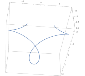
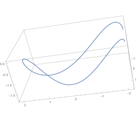
Figure 1: The $f$-rectifying curve $\alpha$ with $f(t)=\sec^{2}t$.

Example 8

Let’s take $Y(t)=\frac{1}{\sqrt{2}}\left(\sin t,\sin t,\sqrt{2}\cos t\right)\in\mathbb{S}^{2}$ and let $f(t)=2t$ where its primitive function is$\ F(t)=t^{2}$ (here we take $t_{0}=0$ and $c=1$), with the inverse $F^{-1}(t)=\sqrt{\left|t\right|}.$
Substituting the values of $f$ and $F$ in Eq.(10)

$$\alpha(t) = \tfrac{\sec t}{2\sqrt{\tan t}}Y(t)-\int\left(\frac{1}{2\sqrt{\tan t}}\right)^{\prime}\sec(t)Y(t)dt$$

$$= \left(\begin{array}[]{c}\sqrt{2}\sqrt{\tan t}+\sqrt{\frac{2}{\cot 2t+\sec 2t}}\\ \sqrt{2}\sqrt{\tan t}+\sqrt{\frac{2}{\cot 2t+\sec 2t}}\\ \frac{1}{2}\sqrt{\cot t}-\frac{1}{2}\sqrt{\cot 2t+\sec 2t}\end{array}\right)$$

is a $f$-rectifying curve for $f(t)=2t$.

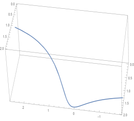
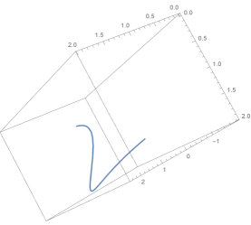
Figure 2: The $f$-rectifying curve $\alpha$ with $f(t)=2t$.

Example 9

For vector $Y(t)=\frac{1}{\sqrt{2}}\left(\sin t,\sin t,\sqrt{2}\cos t\right)$ in $\mathbb{S}^{2}.$ Let $f$ be an integrable function given by $f(t)=e^{t}$, its primitive function is$\ F(t)=e^{t}$ (here we take $c_{1}=0$ and $c=1$), with the inverse $F^{-1}(t)=\ln\left|t\right|.$
Substituting the values of $f$ and $F$ in Eq.(10), the curve $\alpha$

$$\alpha(t) = \tfrac{\sec t}{\tan t}Y(t)-\int\left(\cot t\right)^{\prime}\sec(t)\ Y(t)dt$$

$$= \left(\begin{array}[]{c}\frac{1}{\sqrt{2}}+\frac{1}{2\sqrt{2}}\left(\ln\left(\frac{1-\cos t}{1+\cos t}\right)+2\csc t\right)\\ \frac{1}{\sqrt{2}}+\frac{1}{2\sqrt{2}}\left(\ln\left(\frac{1-\cos t}{1+\cos t}\right)+2\csc t\right)\\ \cot t-\frac{1}{2}\left(\ln\left(\frac{1-\sin t}{1+\sin t}\right)+2\sec t\right)\end{array}\right)$$

is a $f$-rectifying curve for $f(t)=e^{t}$.

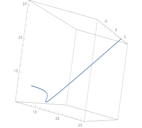
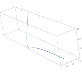
Figure 3: The $f$-rectifying curve $\alpha$ with $f(t)=e^{t}$.

References

- [1] Y. Aminov, Differential Geometry and Topology of Curves, CRC Press, Boca Raton, (2000).
- [2] P. Appell, Traité de Mécanique Rationnelle, vol. 1, 6th ed., Gauthier-Villars,Paris, (1941).
- [3] M. Barros, General helices and a theorem Lancert, Proc Am Math Soc., 125(1997), 1503-1509.
- [4] B. Y. Chen, When does the position vector of a space curve always lie in its rectifying plane?, Amer. Math. Monthly, 110(2003), 147-152 .
- [5] B. Y. Chen and F. Dillen, Rectifying curves as centrodes and extremal curves, Bull. Inst. Math. Academia Sinica, 33(2)(2005), 77-90.
- [6] S. Deshmukhb, Y. Chen and S. H. Alshammari, On rectifying curves in Euclidean 3-space, Turk J. Math., 42(2018), 609-620.
- [7] T. Ikawa, On Some Curves in Riemannian Geometry, Soochow J. Math., 7(1980), 37-44.
- [8] D. A. Singer, Curves whose curvature depends on distance from the origin, this Monthly, 106(1999), 835-841.
- [9] D.J. Struik, Lectures on Classical Differential Geometry, Dover, New-York, (1988).
- [10] J. L. Weiner, How helical can a closed, twisted space curve be?, this Monthly, 107(2000), 327-333.
- [11] H. Yeh and J.I. Abrams, Principles of Mechanics of Solids and Fluids, McGraw-Hall, New York, 1(1960).