Prospects of searching for composite resonances at the LHC and beyond

Abstract

Composite Higgs models predict the existence of resonances. We study in detail the collider phenomenology of both the vector and fermionic resonances, including the possibility of both of them being light and within the reach of the LHC. We present current constraints from di-boson, di-lepton resonance searches and top partner pair searches on a set of simplified benchmark models based on the minimal coset $SO(5)/SO(4)$, and make projections for the reach of the HL-LHC. We find that the cascade decay channels for the vector resonances into top partners, or vice versa, can play an important role in the phenomenology of the models. We present a conservative estimate for their reach by using the same-sign di-lepton final states. As a simple extrapolation of our work, we also present the projected reach at the 27 TeV HE-LHC and a 100 TeV $pp$ collider.

I Introduction

A promising way of addressing the naturalness problem is to consider the existence of strong dynamics around several to 10 TeV scale. The Higgs boson is a pseudo-Nambu-Goldstone boson, much like the pions in the QCD. This so-called composite Higgs scenario Kaplan (1991); Kaplan and Georgi (1984); Contino et al. (2003) has become a main target for the search of new physics at the Large Hadron Collider (LHC).

A generic prediction of the composite Higgs scenario is the presence of composite resonances. Frequently considered resonances are either spin 1, analogous to $\rho$-meson in QCD, or spin $1/2$ resonances with quantum numbers similar to those of the top quark, called “top partners”. In this paper, we study in detail the collider phenomenology of both kinds of resonances. We focus on the minimal coset $SO(5)/SO(4)$, denoted as the Minimal Composite Higgs Model (MCHM) Agashe et al. (2005); Contino et al. (2007). We included several benchmark choices of both the spin 1 resonance and the top partner: $\rho_{L}(\textbf{3},\textbf{1})$, $\rho_{R}(\textbf{1},\textbf{3})$, $\rho_{X}(\textbf{1},\textbf{1})$, $\Psi_{\textbf{4}}(\textbf{2},\textbf{2})$ and $\Psi_{\textbf{1}}(\textbf{1},\textbf{1})$. We derive the current constraints, and make projections for the reach of HL-LHC. We also make a simple extrapolation to estimate the prospectives at the 27 TeV HE-LHC Zimmermann (2017) and the 100 TeV $pp$ collider Arkani-Hamed et al. (2016); CEP (2015); Golling et al. (2017); Contino et al. (2017). Search channels in which the composite resonances are produced via Drell-Yan process and then decay into the Standard Model (SM) final states, such as di-lepton, di-jet, $t\bar{t}$ and di-boson, are well known. We update the limits by including the newest results at the 13 TeV LHC, such as the boosted di-boson jet resonance searches performed by ATLAS with integrated luminosity $L=$ 79.8 fb^-1 ATL (2018a), the di-lepton resonance search at CMS with integrated luminosity $L=77.3~{}{\rm fb}^{-1}$ for the electron channel and $L=36.3~{}{\rm fb}^{-1}$ for the muon channel CMS (2018a), and the search for the pair production of top quark partners with charge-$5/3$ at CMS with integrated luminosity $L=35.9$ fb^-1 Sirunyan et al. (2018a). In addition, we paid close attention to scenarios in which the spin-1 resonances and top partners can be comparable in mass. In this case, cascade decays in which one composite resonance decays into another, can play an important role Greco and Liu (2014); Niehoff et al. (2016); Yepes and Zerwekh (2018a); Barducci et al. (2013); Barducci (2014); Yepes and Zerwekh (2018b). In particular, the channels $\rho^{+}_{L}\rightarrow t\bar{B}/X_{5/3}\bar{t}$ or $\rho^{+}_{L}\rightarrow X_{5/3}\bar{X}_{2/3}$ and $\rho^{0}_{L}\rightarrow X_{5/3}\bar{X}_{5/3}$ can have significant branching ratios for models with quartet top partner, if $\rho_{L}$ is in the intermediate mass region $M_{\Psi}<M_{\rho}<2M_{\Psi}$ or the high mass region $M_{\rho}>2M_{\Psi}$, respectively. Such cascade decays can lead to the same-sign di-lepton (SSDL) signals. Since these are relative clean signals, which have already been used for LHC searches, we use them in our recast and estimate the prospective reach on the $M_{\rho}-M_{\Psi}$ plane. They are comparable in some regions of the parameter space to the di-boson searches for the spin-1 resonances and the pair-produced top partner searches at the LHC. For the models with a singlet top partner, the cascade decay channel $\widetilde{T}\rightarrow t\rho_{X}\rightarrow t\bar{t}t$ in the single production channel can play an important role in the mass region $M_{\widetilde{T}}>M_{\rho_{X}}$. The reach at the LHC is also estimated in the SSDL channels. The projections made based on only the SSDL channel are of course conservative. Other decay modes of the cascade decay channels mentioned above can further enhance the reach, such as the ones including more complicated final states like $1\ell+{\rm jets}$ channels. We leave a detailed exploration of such additional channels for a future work.

The paper is organized as follows. In Section II, we summarize the main phenomenological features of the models, including the couplings of the particles in the mass eigenstates, and the production and the decay of the resonances. The details of the models are presented in Appendix A and Appendix B. In Section III, we show the present bounds from the LHC searches and extrapolate the results to the HL-LHC with an integrated luminosity of $L=3$ ab^-1. An estimate of the reach at the 27 TeV HE-LHC and 100 TeV $pp$ collider is also included. We conclude in Section IV.

II Phenomenology of the models

We begin with a brief review of the composite Higgs models under consideration. We will describe the particle content, and give a qualitative discussion of the sizes of various couplings. The details of the models are presented in Appendix A and  B.

We will consider models similar to those presented in Ref. Greco and Liu (2014). The strong dynamics is assumed to have a global symmetry $SO(5)$, which is broken spontaneously to $SO(4)\simeq SU(2)_{L}\times SU(2)_{R}$. The resulting Goldstone bosons, parameterizing the coset $SO(5)/SO(4)$, contain the Higgs doublet. This is the minimal setup with a custodial $SU(2)$ symmetry. The composite resonances furnish complete representations of $SO(4)$.

Particle content
$\rho_{L}$ $\rho_{R}$ $\rho_{X}$ $\Psi_{\textbf{4}}$ $\Psi_{\textbf{1}}$ $q_{L}^{\textbf{5}}$ $t_{R}^{\textbf{5}}$ $t_{R}^{\rm(F)}$ $SO(4)\simeq SU(2)_{L}\times SU(2)_{R}$ (3,1) (1,3) (1,1) (2,2) (1,1) (2,2) (1,1) (1,1)
Models considered
Interaction $\rho_{L},\Psi_{\mathbb{4}}$ $\rho_{R},\Psi_{\mathbb{4}}$ $\rho_{X},\Psi_{\mathbb{4}}$ $\rho_{X},\Psi_{\textbf{1}}$ Model LP(F)${}_{\textbf{4}}$ RP(F)${}_{\textbf{4}}$ XP(F)${}_{\textbf{4}}$ XP(F)${}_{\textbf{1}}$

Table 1: Upper table: the particle content considered in this paper and their representations under the unbroken $SO(4)\simeq SU(2)_{L}\times SU(2)_{R}$. The SM left-handed quarks $q_{L}=(t_{L},b_{L})^{T}$ are embedded into an incomplete representation, 5, of $SO(5)$. We consider two possible origins of the right-handed top quark. It can be partially composite, denoted as $t_{R}^{\rm(P)}$, and it is embedded in an incomplete representation, 5, of $SO(5)$. It can also be a fully composite resonance, denoted as $t_{R}^{\rm(F)}$, and it is assumed to be an $SO(4)$ singlet massless bound state. Their representations under the unbroken $SO(4)$ are also presented in the table. Lower table: the models with different combinations of the composite spin-1 resonances $\rho$ and the fermionic resonances $\Psi$ considered in our paper. P (F) denotes the partially (fully) composite right-handed top quark.

We summarize the particle content and the models considered in our paper in Table 1. For the spin-1 resonances $\rho$, we consider three representations under the unbroken $SO(4)\simeq SU(2)_{L}\times SU(2)_{R}$: $\rho_{L}(\textbf{3},\textbf{1})$, $\rho_{R}(\textbf{1},\textbf{3})$, $\rho_{X}(\textbf{1},\textbf{1})$, while for the fermionic resonances $\Psi$, we study the quartet $\Psi_{\textbf{4}}(\textbf{2},\textbf{2})$ and the singlet $\Psi_{\textbf{1}}(\textbf{1},\textbf{1})$. The left handed SM fermions, $q_{L}=(t_{L},b_{L})^{T}$, are assumed to be embedded into (incomplete) 5 representations of $SO(5)$ (see Eq. (47)) Contino et al. (2007). There are two well-studied ways of dealing with the right handed top quark. First, it can be treated as an elementary field, and embedded into a 5 representation of $SO(5)$ (see Eq. (48)) Contino et al. (2007). We call this the partially composite right-handed top quark scenario, and denote right-handed top as $t^{\rm(P)}_{R}$. It is also possible that it is a massless bound state of the strong sector and a $SO(4)$ singlet, denoted as $t_{R}^{\rm(F)}$ De Simone et al. (2013). We call this the fully composite right-handed top quark scenario. We will consider both of these cases. In principle, many of the composite resonances can be comparable in their masses in a given model. Rather than getting in the numerous combinations, we consider a set of simplified models in which only one kind of spin-1 resonance(s) and one kind of top partner(s) are light and relevant for collider searches. For example, model LP${}_{\textbf{4}}$ involves the strong interactions between the $\rho_{L}$ and the quartet top partner $\Psi_{\textbf{4}}$ and the partially composite right-handed top quark. In comparison, model LF${}_{\textbf{4}}$ is different only in the treatment of the right handed top quark which is assumed to be fully composite.

In the following, we will first discuss all the most relevant interactions and their coupling strengths in Section II.1. The production and decay of the resonances at the LHC are presented in Section II.2. The mass matrices of different models and their diagonalizations are discussed in Appendix C, where we also list the expressions all the mass eigenvalues.

II.1 The couplings

Scale $f$, similar to the pion decay constant in QCD, parameterizes the size of global symmetry breaking. The parameter $\xi=v^{2}/f^{2}$ measures the hierarchy between the weak scale and the global symmetry breaking scale in the strong sector. It has been well constrained from LEP electroweak precision test (EWPT) and the LHC Higgs coupling measurements to be $\xi\lesssim 0.13$ Sanz and Setford (2018); de Blas et al. (2018). In the expressions for the couplings, we will keep only terms to the leading order in $\xi$.

The interactions of the spin-1 resonances in the strong sector are characterized by several couplings, $(g_{\rho_{L}},g_{\rho_{R}},g_{\rho_{X}})$, sometimes collectively denoted as $g_{\rho}$. Typically, they are assumed to be much larger than the SM gauge couplings, i.e. $g_{\rho}\gg g^{\prime}$, $g$. We will keep only terms to the leading order in $g/g_{\rho}$ in the expressions of the couplings . Similar to Ref. Contino et al. (2011), we will also introduce an $\mathcal{O}(1)$ parameter for each representation of the spin-1 resonances, defined as

$$a_{\rho_{L,R,X}}=\frac{m_{\rho_{L,R,X}}}{g_{\rho_{L,R,X}}f}.$$ (1)

In most of the cases, we will fix $a_{\rho}$.

The sector of fermionic composite resonances involve another strong coupling, $g_{\Psi}$, defined as:

$$g_{\Psi}=\frac{M_{\Psi}}{f},\quad M_{\Psi}=M_{\textbf{4}},~{}M_{\textbf{1}}.$$ (2)

For partially composite SM fermions, there are mixings between the SM fermions and the top partners before electroweak symmetry breaking (EWSB). For example, the mixing angles between the elementary left (right) handed top and the quartet (singlet) top partners (defined in Eq. (59) and Eq. (86)) in models within the partially composite right-handed top quark scenario are:

$$s_{\theta_{L}}\equiv\sin\theta_{L}=\frac{y_{L}f}{\sqrt{M_{\textbf{4}}^{2}+y_{L}^{2}f^{2}}},\quad s_{\theta_{R}}\equiv\sin\theta_{R}=\frac{y_{R}f}{\sqrt{M_{\textbf{1}}^{2}+y_{R}^{2}f^{2}}}.$$ (3)

and the same definition applies to $c_{\theta_{L}}$, $c_{\theta_{R}}$, $t_{\theta_{L}}$, $t_{\theta_{R}}$. The interactions of the spin-1 resonances and the fermions are summarized in Table 2 (for the charged sector) and Table 3, Table 4 (for the neutral sector).

Vertices	$\rho_{L}^{+}$	$\rho_{R}^{+}$	$W^{+}$
Between heavy resonances:
$\begin{array}[]{cccc}\bar{T}_{R}B_{R},\bar{X}_{5/3R}X_{2/3R}\\ \bar{X}_{5/3L}X_{2/3L}\end{array}$	$\begin{array}[]{cc}\frac{c_{1}}{\sqrt{2}}g_{\rho_{L}}\end{array}$	$\mathcal{O}(g_{\rho_{R}}\xi)$	$\frac{g}{\sqrt{2}}$
$\bar{T}_{L}B_{L}$	$\begin{array}[]{cc}\frac{c_{1}}{\sqrt{2}}g_{\rho_{L}}c_{\theta_{L}}^{2}\end{array}$	$\mathcal{O}(g_{\rho_{R}}\xi)$	$\frac{g}{\sqrt{2}}$
$\bar{X}_{2/3R}B_{R},\bar{X}_{5/3R}T_{R}$	$\mathcal{O}(g_{\rho_{L}}\xi)$	$c_{1}\frac{g_{\rho_{R}}}{\sqrt{2}}\,$	$\mathcal{O}(g\xi)$
$\bar{X}_{2/3L}B_{L},\bar{X}_{5/3L}T_{L}$	$\mathcal{O}(g_{\rho_{L}}\xi)$	$c_{1}\frac{g_{\rho_{R}}}{\sqrt{2}}\,c_{\theta_{L}}$	$\mathcal{O}(g\xi)$
Between heavy resonances and SM fermions:
$\bar{T}_{L}b_{L},\bar{t}_{L}B_{L}$	$\frac{c_{1}}{\sqrt{2}}g_{\rho_{L}}c_{\theta_{L}}s_{\theta_{L}}$	$\mathcal{O}(g_{\rho_{R}}\xi)$	$\mathcal{O}(g\xi)$
$\bar{X}_{2/3L}b_{L},\bar{X}_{5/3L}t_{L}$	$\mathcal{O}(g_{\rho_{L}}\xi)$	$c_{1}\frac{g_{\rho_{R}}}{\sqrt{2}}\,s_{\theta_{L}}$	$\mathcal{O}(g\xi)$
$\bar{t}_{R}B_{R}$	$\frac{y_{R}s_{\theta_{L}}c_{\theta_{L}}}{2y_{L}}c_{1}g_{\rho_{L}}\sqrt{\xi}$ (P)	$-\frac{y_{R}t_{\theta_{L}}}{2y_{L}}c_{1}g_{\rho_{R}}\sqrt{\xi}$ (P)	$\frac{y_{R}s_{\theta_{L}}c_{\theta_{L}}}{2y_{L}}g\sqrt{\xi}$ (P)
	$\frac{y_{2L}s_{\theta_{L}}^{2}}{2y_{L}}c_{1}g_{\rho_{L}}\sqrt{\xi}$ (F)	$\mathcal{O}(\xi^{3/2})$ (F)	$\frac{y_{2L}s_{\theta_{L}}^{2}}{2y_{L}}g\sqrt{\xi}$ (F)
$\bar{X}_{5/3R}t_{R}$	$-\frac{y_{R}t_{\theta_{L}}}{2y_{L}}c_{1}g_{\rho_{L}}\sqrt{\xi}$ (P)	$\frac{y_{R}s_{\theta_{L}}c_{\theta_{L}}}{2y_{L}}c_{1}g_{\rho_{R}}\sqrt{\xi}$ (P)	$-\frac{y_{R}t_{\theta_{L}}}{2y_{L}}g\sqrt{\xi}$ (P)
	$c_{2}\frac{g^{2}}{\sqrt{2}g_{\rho_{L}}}\sqrt{\xi}$ (F)	$\frac{y_{2L}s_{\theta_{L}}^{2}}{2y_{L}}c_{1}g_{\rho_{R}}\sqrt{\xi}$ (F)	$-c_{2}\frac{g^{2}}{\sqrt{2}}\sqrt{\xi}$(F)
Between SM particles:
$i\phi^{-}\mathord{\buildrel\lower 3.0pt\hbox{$\scriptscriptstyle\leftrightarrow$}\over{\partial}_{\mu}}\phi^{0}$ a	$\frac{1}{\sqrt{2}}a_{\rho_{L}}^{2}g_{\rho_{L}}$	$-\frac{a_{\rho_{R}}^{2}g_{\rho_{R}}}{\sqrt{2}}$	$\frac{g}{\sqrt{2}}$
$\bar{t}_{L}b_{L}$	$\begin{array}[]{cc}\frac{1}{\sqrt{2}}\left(c_{1}g_{\rho_{L}}s_{\theta_{L}}^{2}-\frac{g^{2}}{g_{\rho_{L}}}\right)\end{array}$	$\mathcal{O}(g_{\rho_{R}}\xi)$	$\frac{g}{\sqrt{2}}$
$\bar{f}_{\text{el},L}f^{\prime}_{\text{el},L}$	$-\frac{1}{\sqrt{2}}\frac{g^{2}}{g_{\rho_{L}}}$	$\mathcal{O}\left(\frac{g^{2}}{g_{\rho_{R}}}\xi\right)$	$\frac{g}{\sqrt{2}}$

• For $\rho_{R}^{+}$, it should be $i\phi^{-}\mathord{\buildrel\lower 3.0pt\hbox{$\scriptscriptstyle\leftrightarrow$}\over{\partial}_{\mu}}\phi^{0*}.$

Table 2: The LO coupling strengths between the charged spin-1 bosons $\rho^{\pm}_{L,R}$, $W^{\pm}$ and the fermions in models LP(F)${}_{\textbf{4}}$, RP(F)${}_{\textbf{4}}$. Note that $f_{\text{el}}$ denotes all the SM light fermions, including the first two generation quarks, $b_{R}$ and all the leptons. Here (P) and (F) mean the partially and fully composite right-handed top quark scenario, respectively.

Vertices	$\rho_{L}^{0}$	$\rho_{R}^{0}$	$\rho_{X}^{0}$	$Z$
Between heavy resonances:
$\begin{array}[]{cccccccccc}\bar{X}_{5/3}X_{5/3},\bar{T}_{R}T_{R}\\ \bar{X}_{2/3}X_{2/3},\bar{B}_{R}B_{R}\end{array}$	$\begin{array}[]{cc}T^{3_{L}}c_{1}g_{\rho_{L}}\end{array}$	$\begin{array}[]{cccccccccc}T^{3_{R}}c_{1}g_{\rho_{R}}\end{array}$	$\begin{array}[]{cc}c_{1}g_{\rho_{X}}\end{array}$	$\begin{array}[]{ccc}\frac{g}{c_{W}}\left(T^{3_{L}}-Qs_{W}^{2}\right)\end{array}$
$\begin{array}[]{cccccccccc}\bar{X}_{2/3L}T_{L},\bar{T}_{L}X_{2/3L}\end{array}$	$\begin{array}[]{cc}\mathcal{O}(g_{\rho_{L}}\xi)\end{array}$	$\begin{array}[]{cccccccccc}\mathcal{O}(g_{\rho_{R}}\xi)\end{array}$	$\begin{array}[]{cc}\mathcal{O}(g_{\rho_{X}}\xi)\end{array}$	$\begin{array}[]{ccc}\mathcal{O}(g\xi)\end{array}$
$\begin{array}[]{cccccccccc}\bar{X}_{2/3R}T_{R},\bar{T}_{R}X_{2/3R}\end{array}$	$\begin{array}[]{cc}\mathcal{O}(g_{\rho_{L}}\xi)\end{array}$	$\begin{array}[]{cccccccccc}\mathcal{O}(g_{\rho_{R}}\xi)\end{array}$	$\begin{array}[]{cc}\mathcal{O}(g_{\rho_{X}}\xi)\end{array}$	$\begin{array}[]{ccc}\mathcal{O}(g\xi)\end{array}$
$\bar{T}_{L}T_{L},\bar{B}_{L}B_{L}$	$\begin{array}[]{cc}T^{3_{L}}c_{1}g_{\rho_{L}}c_{\theta_{L}}^{2}\end{array}$	$\begin{array}[]{cccccccccc}-\frac{1}{2}c_{1}g_{\rho_{R}}c_{\theta_{L}}^{2}\end{array}$	$\begin{array}[]{cc}c_{1}g_{\rho_{X}}c_{\theta_{L}}^{2}\end{array}$	$\begin{array}[]{ccc}\frac{g}{c_{W}}\left(T^{3_{L}}-Qs_{W}^{2}\right)\end{array}$
Between heavy resonances and SM fermions:
$\begin{array}[]{cccccccccc}\bar{T}_{L}t_{L},\bar{B}_{L}b_{L}\\ \bar{t}_{L}T_{L},\bar{b}_{L}B_{L}\end{array}$	$\begin{array}[]{cc}T^{3_{L}}c_{1}g_{\rho_{L}}s_{\theta_{L}}c_{\theta_{L}}\end{array}$	$-\frac{1}{2}c_{1}g_{\rho_{R}}s_{\theta_{L}}c_{\theta_{L}}$	$\begin{array}[]{cc}c_{1}g_{\rho_{X}}s_{\theta_{L}}c_{\theta_{L}}\end{array}$	$\begin{array}[]{cccccccccc}\mathcal{O}(g\xi)\end{array}$
$\bar{T}_{R}t_{R},\bar{t}_{R}T_{R}$	$\frac{y_{R}s_{\theta_{L}}c_{\theta_{L}}}{2\sqrt{2}y_{L}}c_{1}g_{\rho_{L}}\sqrt{\xi}$ (P)	$-\frac{y_{R}s_{\theta_{L}}c_{\theta_{L}}}{2\sqrt{2}y_{L}}c_{1}g_{\rho_{R}}\sqrt{\xi}$ (P)	$\frac{y_{R}s_{\theta_{L}}c_{\theta_{L}}}{\sqrt{2}y_{L}}c_{1}g_{\rho_{X}}\sqrt{\xi}$ (P)	$\frac{y_{R}s_{\theta_{L}}c_{\theta_{L}}}{2\sqrt{2}y_{L}}\frac{g}{s_{w}}\sqrt{\xi}$ (P)
	$\frac{y_{2L}s_{\theta_{L}}^{2}}{2\sqrt{2}y_{L}}c_{1}g_{\rho_{L}}\sqrt{\xi}$ (F)	$-\frac{y_{2L}s_{\theta_{L}}^{2}}{2\sqrt{2}y_{L}}c_{1}g_{\rho_{R}}\sqrt{\xi}$ (F)	$\frac{y_{2L}s_{\theta_{L}}^{2}}{\sqrt{2}y_{L}}(c_{1}-c_{1}^{\prime})g_{\rho_{X}}\sqrt{\xi}$ (F)	$\frac{y_{2L}s_{\theta_{L}}^{2}}{2\sqrt{2}y_{L}}\frac{g}{c_{w}}\sqrt{\xi}$ (F)
$\begin{array}[]{cccccccccc}\bar{X}_{2/3L}t_{L},\bar{t}_{L}X_{2/3L}\end{array}$	$\begin{array}[]{cc}\mathcal{O}(g_{\rho_{L}}\xi)\end{array}$	$\begin{array}[]{cccccccccc}\mathcal{O}(g_{\rho_{R}}\xi)\end{array}$	$\begin{array}[]{cc}\mathcal{O}(g_{\rho_{X}}\xi)\end{array}$	$\begin{array}[]{ccc}\mathcal{O}(g\xi)\end{array}$
$\bar{X}_{2/3R}t_{R},\bar{t}_{R}X_{2/3R}$	$\frac{y_{R}t_{\theta_{L}}}{2\sqrt{2}y_{L}}c_{1}g_{\rho_{L}}\sqrt{\xi}$ (P)	$-\frac{y_{R}t_{\theta_{L}}}{2\sqrt{2}y_{L}}c_{1}g_{\rho_{R}}\sqrt{\xi}$ (P)	$-\frac{y_{R}t_{\theta_{L}}}{\sqrt{2}y_{L}}c_{1}g_{\rho_{X}}\sqrt{\xi}$ (P)	$\frac{y_{R}t_{\theta_{L}}}{2\sqrt{2}y_{L}}\frac{g}{c_{w}}\sqrt{\xi}$ (P)
	$c_{2}\frac{g^{2}}{2g_{\rho_{L}}}\sqrt{\xi}$ (F)	$c_{2}\frac{g^{\prime 2}}{2g_{\rho_{L}}}\sqrt{\xi}$ (F)	$\frac{c_{2}}{2}\frac{g}{c_{W}}\sqrt{\xi}$ (F)	$\mathcal{O}(\xi^{3/2})$ (F)
Between SM particles:
$i\phi^{-}\mathord{\buildrel\lower 3.0pt\hbox{$\scriptscriptstyle\leftrightarrow$}\over{\partial}_{\mu}}\phi^{+}$	$\begin{array}[]{cccccccccc}\frac{1}{2}a_{\rho_{L}}^{2}g_{\rho_{L}}\end{array}$	$\begin{array}[]{cccccccccc}\frac{1}{2}a_{\rho_{R}}^{2}g_{\rho_{R}}\end{array}$	$-\frac{1}{2}\frac{g^{\prime 2}}{g_{\rho_{X}}}$	$\frac{g}{c_{W}}\left(\frac{1}{2}-s_{W}^{2}\right)$
$i\phi^{0*}\mathord{\buildrel\lower 3.0pt\hbox{$\scriptscriptstyle\leftrightarrow$}\over{\partial}_{\mu}}\phi^{0}$	$\begin{array}[]{cccccccccc}-\frac{1}{2}a_{\rho_{L}}^{2}g_{\rho_{L}}\end{array}$	$\begin{array}[]{cccccccccc}\frac{1}{2}a_{\rho_{R}}^{2}g_{\rho_{R}}\end{array}$	$-\frac{1}{2}\frac{g^{\prime 2}}{g_{\rho_{X}}}$	$-\frac{g}{2c_{W}}$
$\bar{t}_{L}t_{L},\bar{b}_{L}b_{L}$	$\begin{array}[]{cc}T^{3_{L}}\left(c_{1}g_{\rho_{L}}s_{\theta_{L}}^{2}-\frac{g^{2}}{g_{\rho_{L}}}\right)\end{array}$	$-\frac{1}{2}c_{1}g_{\rho_{R}}s_{\theta_{L}}^{2}-\frac{1}{6}\frac{g^{\prime 2}}{g_{\rho_{R}}}$	$\begin{array}[]{cc}c_{1}g_{\rho_{X}}s_{\theta_{L}}^{2}-\frac{1}{6}\frac{g^{\prime 2}}{g_{\rho_{X}}}\end{array}$	$\begin{array}[]{cccccccccc}\frac{g}{c_{W}}\left(T^{3_{L}}-Qs_{W}^{2}\right)\\ +\mathcal{O}(g\xi){\textsuperscript{\emph{a}}}\end{array}$
$\bar{t}_{R}t_{R}$	$\mathcal{O}(g_{\rho_{L}}\xi)$	$-\frac{2}{3}\frac{g^{\prime 2}}{g_{\rho_{R}}}+\mathcal{O}(g_{\rho_{R}}\xi)$	$\begin{array}[]{cccccccccc}c_{1}^{\prime}g_{\rho_{X}}(\text{F})\\ -\frac{2}{3}\frac{g^{\prime 2}}{g_{\rho_{X}}}+\mathcal{O}(g_{\rho_{X}}\xi)(\text{P})\end{array}$	$-\frac{2gs_{W}^{2}}{3c_{W}}+\mathcal{O}(g\xi)$
$\bar{f}_{\text{el}}f_{\text{el}}$	$-T^{3_{L}}\frac{g^{2}}{g_{\rho_{L}}}$	$-Y\frac{g^{\prime 2}}{g_{\rho_{R}}}$	$-Y\frac{g^{\prime 2}}{g_{\rho_{X}}}$	$\frac{g}{c_{W}}\left(T^{3_{L}}-Qs_{W}^{2}\right)$

• For model LP(F)${}_{\textbf{4}}$ and RP(F)${}_{\textbf{4}}$, it reads $\frac{g}{4c_{W}}\left[-T^{3_{L}}-\frac{1}{2}\right]s_{\theta_{L}}^{2}\xi$.

Table 3: The LO coupling strengths between the neutral spin-1 bosons, $\rho^{0}_{L,R,X}$ and $Z$, and the fermions in models LP(F)${}_{\textbf{4}}$, RP(F)${}_{\textbf{4}}$, and XP(F)${}_{\textbf{4}}$. $f_{\text{el}}$ denotes all the SM elementary fermions including the first two generation quarks, $b_{R}$ and all the leptons. Here (P) and (F) in the couplings refer to the partially and fully composite right-handed top quark scenario, respectively. $c_{W}$ denotes $\cos\theta_{W}$ with $\theta_{W}$ being the weak mixing angle.

Vertices	$\overline{\widetilde{T}}_{L}\widetilde{T}_{L}$	$\overline{\widetilde{T}}_{L}t_{L},\bar{t}_{L}\widetilde{T}_{L}$	$\bar{t}_{L}t_{L}$	$\overline{\widetilde{T}}_{R}\widetilde{T}_{R}$	$\overline{\widetilde{T}}_{R}t_{R},\bar{t}_{R}\widetilde{T}_{R}$	$\bar{t}_{R}t_{R}$	$\bar{b}_{L}b_{L}$
$\rho_{X}^{0}$ (XP${}_{\textbf{1}}$)	$\begin{array}[]{ccc}c_{1}g_{\rho_{X}}\end{array}$	$-\frac{y_{L}c_{\theta_{R}}s_{\theta_{R}}}{\sqrt{2}y_{R}}c_{1}g_{\rho_{X}}\sqrt{\xi}$	$-\frac{1}{6}\frac{g^{\prime 2}}{g_{\rho_{X}}}$	$c_{1}g_{\rho_{X}}c_{\theta_{R}}^{2}$	$\begin{array}[]{ccc}c_{1}g_{\rho_{X}}\,s_{\theta_{R}}c_{\theta_{R}}\end{array}$	$\begin{array}[]{cccccccccc}c_{1}g_{\rho_{X}}s_{\theta_{R}}^{2}\\ -\frac{2}{3}\frac{g^{\prime 2}}{g_{\rho_{X}}}\end{array}$	$-\frac{1}{6}\frac{g^{\prime 2}}{g_{\rho_{X}}}$
$\rho_{X}^{0}$ (XF${}_{\textbf{1}}$)	$\begin{array}[]{ccc}c_{1}g_{\rho_{X}}\end{array}$	$-\frac{y_{L}f}{\sqrt{2}M_{1}}c_{1}g_{\rho_{X}}\sqrt{\xi}$	$-\frac{1}{6}\frac{g^{\prime 2}}{g_{\rho_{X}}}$	$\begin{array}[]{ccc}c_{1}g_{\rho_{X}}\end{array}$	$\begin{array}[]{ccc}c_{1}^{\prime\prime}g_{\rho_{X}}\end{array}$	$\begin{array}[]{cccccccccc}c_{1}^{\prime}g_{\rho_{X}}\end{array}$	$-\frac{1}{6}\frac{g^{\prime 2}}{g_{\rho_{X}}}$
$Z$	$-\frac{2gs_{W}^{2}}{3c_{W}}$	$\begin{array}[]{cccccccccc}\frac{y_{L}c_{\theta_{R}}s_{\theta_{R}}}{\sqrt{2}y_{R}}\frac{g}{2c_{W}}\sqrt{\xi}~{}(\text{XP}_{\textbf{1}})\\ \frac{y_{L}f}{\sqrt{2}M_{1}}\frac{g}{2c_{W}}\sqrt{\xi}~{}(\text{XF}_{\textbf{1}})\end{array}$	$\frac{g}{c_{W}}\left(\frac{1}{2}-\frac{2s_{W}^{2}}{3}\right)$	$-\frac{2gs_{W}^{2}}{3c_{W}}$	0	$-\frac{2gs_{W}^{2}}{3c_{W}}$	$\frac{g}{c_{W}}\left(-\frac{1}{2}+\frac{s_{W}^{2}}{3}\right)$

Table 4: The LO coupling strengths between the neutral spin-1 gauge bosons, $\rho^{0}_{X}$ and $Z$, and the fermions in models XP(F)${}_{\textbf{1}}$.

The couplings can be organized into four classes by their typical sizes. The first class includes the interactions generated directly from the strong dynamics and preserve the non-linearly realized $SO(5)$ symmetry. They only involve the strong sector resonances $\rho$, $\Psi$, the pseudo-Goldstone bosons $\vec{h}$ and the fully composite right-handed top quark $t_{R}^{\rm(F)}$. The interaction strengths are of $\mathcal{O}(g_{\rho})$ or $\mathcal{O}(g_{\Psi})$. Since these interactions preserve the unbroken $SO(4)$ symmetry, the interactions between $\rho$ and $\Psi$ are determined by the quantum number of the fermionic resonances under the $SU(2)_{L}\times SU(2)_{R}$. The symmetry selection rules permit the following interactions of $\mathcal{O}(g_{\rho})$:

$$\rho_{L}^{+}\bar{T}B,\quad\rho_{L}^{+}\bar{X}_{5/3}X_{2/3},\quad\rho_{R}^{+}\bar{X}_{2/3}B,\quad\rho_{R}^{+}\bar{X}_{5/3}T,\quad\rho_{L,R,X}^{0}\bar{\mathcal{T}}\mathcal{T},\quad\rho_{X}^{0}\overline{\widetilde{T}}\widetilde{T},\quad\rho_{X}^{0}\bar{t}_{R}^{\rm(F)}t_{R}^{\rm(F)},$$ (4)

where $\mathcal{T}=T$, $B$, $X_{5/3}$, $X_{2/3}$ denotes the fermionic resonances in the quartet. The last term is for the case of a fully composite right-handed top quark. As will be discussed in the next subsection, these interactions dominate the decay of $\rho$ resonances if the channels are kinematically open. For the interactions involving the $\rho$ and the Higgs doublet $H$, we have (see Appendex B for detail):

$$\frac{a_{\rho_{L}}^{2}}{2}g_{\rho_{L}}\rho^{a_{L}\mu}iH^{\dagger}\sigma^{a_{L}}\mathord{\buildrel\lower 3.0pt\hbox{$\scriptscriptstyle\leftrightarrow$}\over{D}_{\mu}}H,\quad\frac{a_{\rho_{R}}^{2}}{2}g_{\rho_{R}}\rho^{a_{R}\mu}J_{\mu}^{a_{R}}(H),$$ (5)

where we have defined the $SU(2)_{R}$ current

$$J_{\mu}^{a_{R}}(H)=\left(-i\left(\widetilde{H}^{\dagger}D_{\mu}H-D_{\mu}H^{\dagger}\widetilde{H}\right),-\left(H^{\dagger}D_{\mu}\widetilde{H}+D_{\mu}\widetilde{H}^{\dagger}H\right),iH^{\dagger}\mathord{\buildrel\lower 3.0pt\hbox{$\scriptscriptstyle\leftrightarrow$}\over{D}_{\mu}}H\right).$$ (6)

The Higgs doublet can be parameterized as

$$H=\begin{pmatrix}\phi^{+}\\ \phi^{0}\end{pmatrix}=\begin{pmatrix}\phi^{+}\\ \frac{h+i\chi}{\sqrt{2}}\end{pmatrix},$$ (7)

with $\phi^{\pm}$, $\chi$ eaten by the SM $W^{\pm}$, $Z$ bosons after EWSB. By the Goldstone equivalence theorem, the interactions involve $\phi^{\pm}$, $\chi$ will determine the couplings of longitudinal modes of $W^{\pm}$ and $Z$ gauge bosons at high energy, leading to the following interactions with $\mathcal{O}(g_{\rho})$:

$$\begin{split}&\frac{a_{\rho_{L}}^{2}}{2}g_{\rho_{L}}\Big{[}\rho_{L}^{3}(\phi^{-}i\mathord{\buildrel\lower 3.0pt\hbox{$\scriptscriptstyle\leftrightarrow$}\over{\partial}_{\mu}}\phi^{+}-\phi^{0*}i\mathord{\buildrel\lower 3.0pt\hbox{$\scriptscriptstyle\leftrightarrow$}\over{\partial}_{\mu}}\phi^{0})+\sqrt{2}\rho_{L}^{+}\phi^{-}i\mathord{\buildrel\lower 3.0pt\hbox{$\scriptscriptstyle\leftrightarrow$}\over{\partial}_{\mu}}\phi^{0}+\sqrt{2}\rho_{L}^{-}\phi^{0*}i\mathord{\buildrel\lower 3.0pt\hbox{$\scriptscriptstyle\leftrightarrow$}\over{\partial}_{\mu}}\phi^{+}\Big{]},\\ &\frac{a_{\rho_{R}}^{2}}{2}g_{\rho_{R}}\Big{[}\rho_{R}^{3}(\phi^{-}i\mathord{\buildrel\lower 3.0pt\hbox{$\scriptscriptstyle\leftrightarrow$}\over{\partial}_{\mu}}\phi^{+}+\phi^{0*}i\mathord{\buildrel\lower 3.0pt\hbox{$\scriptscriptstyle\leftrightarrow$}\over{\partial}_{\mu}}\phi^{0})+\sqrt{2}\rho_{R}^{+}\phi^{0*}i\mathord{\buildrel\lower 3.0pt\hbox{$\scriptscriptstyle\leftrightarrow$}\over{\partial}_{\mu}}\phi^{-}+\sqrt{2}\rho_{R}^{-}\phi^{+}i\mathord{\buildrel\lower 3.0pt\hbox{$\scriptscriptstyle\leftrightarrow$}\over{\partial}_{\mu}}\phi^{0}\Big{]}.\end{split}$$ (8)

Hence, $\rho_{L,R}$ will primarily decay into the longitudinal gauge bosons and the Higgs bosons if the other strongly interacting decay channels ($\Psi\Psi$ or $\Psi q$) are not kinematically open. The other type in the first class is the interactions between the resonances $\Psi_{\textbf{4}}$ and $t_{R}^{\rm(F)}$ in Eq. (51):

$$c_{2}\bar{\Psi}_{\textbf{4}}^{i}\gamma^{\mu}id^{i}_{\mu}t_{R}^{\rm(F)}=\frac{\sqrt{2}c_{2}}{f}\left(M_{Q_{X}}\bar{Q}_{XL}Ht_{R}^{\rm(F)}-M_{Q}\bar{Q}_{L}\widetilde{H}t_{R}^{\rm(F)}+\text{h.c.}\right)+\cdots,$$ (9)

where we have integrated by parts before turning on the Higgs vacuum expectation value (VEV) and focused only on the trilinear couplings (see Ref. De Simone et al. (2013) for detail). $M_{Q_{X}}$, $M_{Q}$ are defined in Eq. (60). In the limit $M_{\textbf{4}}/f\gg y_{L},y_{2L}$, these are the dominant interactions between the top partners and the SM fields. By using Goldstone equivalence theorem, we can easily derive the well-known approximate decay branching ratios for the top parnters:

$$\begin{split}&\text{Br}(T\rightarrow th)\simeq\text{Br}(T\rightarrow tZ)\simeq 50\%,\quad\text{Br}(X_{2/3}\rightarrow th)\simeq\text{Br}(X_{2/3}\rightarrow tZ)\simeq 50\%,\\ &\text{Br}(X_{5/3}\rightarrow tW)\simeq 100\%,\quad\text{Br}(B\rightarrow tW)\simeq 100\%.\end{split}$$ (10)

Taking into account the mixing effects, shown in Eq. (3), will not modify the conclusions significantly.

The second class of interactions are suppressed either by the left-handed top quark mixing $s_{\theta_{L}}$ or the right-handed top quark mixing $s_{\theta_{R}}$ defined in Eq. (3). These are the couplings of $\rho$ to one top partner and one SM quark. These interactions preserve SM $SU(2)_{L}\times U(1)_{Y}$ gauge symmetries. Symmetry considerations select the following interactions:

$$\rho_{L}^{+}\bar{T}_{L}b_{L},\quad\rho_{L}^{+}\bar{t}_{L}B_{L},\quad\rho_{L,R,X}^{0}\bar{T}_{L}t_{L},\quad\rho_{L,R,X}^{0}\bar{B}_{L}b_{L},\quad\rho_{X}^{0}\overline{\widetilde{T}}_{R}t_{R}^{\rm(P)},$$ (11)

where the last term is only present for the partially composite right-handed top quark scenario. The interactions will play an important role in the kinematical region $M_{\Psi}+M_{t,b}<M_{\rho}<2M_{\Psi}$, if the mixings $s_{\theta_{L,R}}$ are not too small.

The third class of interactions contains the SM gauge interactions with couplings $g$, $g^{\prime}$ or SM Yukawa couplings. These include the $W$ and $Z$ interactions with SM elementary fermions (quarks and the leptons) and the fermionic resonances; and the mixed couplings, proportional to $y_{L,R}$, between the top partners $\Psi_{\textbf{4},\textbf{1}}$ and the elementary SM quarks $q_{L}$, $t_{R}^{\rm(P)}$. The gauge interactions are determined by the SM quantum numbers of the fermions. The Yukawa type interactions in Eq. (65) and Eq. (85) control the decays of the top partners

$$y_{R}\left(\bar{Q}_{L}\widetilde{H}t_{R}^{\rm(P)}-\bar{Q}_{XL}Ht_{R}^{\rm(P)}\right),\quad-y_{L}\bar{q}_{L}\widetilde{H}\widetilde{T}_{R}.$$ (12)

which leads to the same decay branching ratios as Eq. (10) for the quartet. For the singlet top partner, this gives

$$\begin{split}\text{Br}(\widetilde{T}\rightarrow bW^{+})\simeq 2\text{Br}(\widetilde{T}\rightarrow th)\simeq 2\text{Br}(\widetilde{T}\rightarrow tZ)\simeq 50\%.\end{split}$$ (13)

The fourth class contains the interactions with coupling strengths suppressed by $g/g_{\rho}$, $g^{\prime}/g_{\rho}$. These are the universal couplings between the $\rho$ and the SM fermions, due to the mixings of $\rho$ and SM gauge bosons which are present before the EWSB. These interactions include

$$\rho_{L,R}^{+}\bar{f}_{\text{el}}f^{\prime}_{\text{el}},\quad\rho_{L,R,X}^{0}\bar{f}_{\text{el}}f_{\text{el}},$$ (14)

where $f_{\text{el}}$ denotes all the SM elementary fermions including the first two generation quarks, $b_{R}$, and all of the leptons. For the $\rho_{L}$, the couplings are of $\mathcal{O}(g^{2}/g_{\rho_{L}})$, while for $\rho_{R,X}^{0}$, they are of $\mathcal{O}(g^{\prime 2}/g_{\rho_{R,X}})$. For the couplings between $\rho$ and the third generation quarks, there are additional contributions of $\mathcal{O}(g_{\rho}s_{\theta_{L,R}}^{2})$:

$$\rho_{L}^{+}\bar{t}_{L}b_{L},\quad\rho_{L,R,X}^{0}\bar{t}_{L}t_{L},\quad\rho_{L,R,X}^{0}\bar{b}_{L}b_{L},\quad\rho_{X}^{0}\bar{t}_{R}^{\rm(P)}t_{R}^{\rm(P)},$$ (15)

with the final term only arises for the partially composite right-handed top quark. All the remaining coupling vertices can only be present after EWSB. Therefore, they are suppressed further by $\xi$ and irrelevant for the phenomenology of the composite resonances.

II.2 The production and the decay of the resonances at the LHC

In this subsection, we discuss the production and decay of the composite resonances. The cross sections are calculated by first implementing the benchmark models into an UFO model file through the FeynRules Alloul et al. (2014) package and then using MadGraph5_aMC@NLO Alwall et al. (2014) to simulate the processes. Most of the calculations are carried out at the LO. The only exception is the QCD pair production of top partners, for which we use the Top++2.0 package Czakon and Mitov (2014); Czakon et al. (2013); Czakon and Mitov (2013, 2012); Bärnreuther et al. (2012); Cacciari et al. (2012) to obtain the next-to-next-to-leading-order (NNLO) cross sections. See Appendix D for the cross sections at different proton-proton center-of-mass energies. For the decay widths, we have used the analytical formulae calculated by the FeynRules.

II.2.1 Production at the LHC

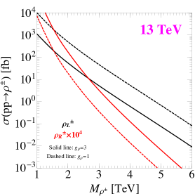
(a)  Charged vector resonances.

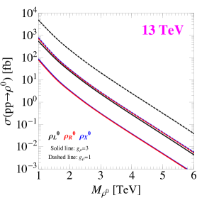
(b)  Neutral vector resonances.

Figure 1: The Drell-Yan cross sections for the vector resonances at the 13 TeV LHC, in the unit of fb. The cross section of $\rho_{R}^{\pm}$ is shown as $\sigma(pp\to\rho_{R}^{\pm})\times 10^{4}$. We have fixed the parameters $a_{\rho_{L,R,X}}^{2}$ (see Eq. (62), Eq. (73) and Eq. (80) for the definitions) equal to $1/2$. The rates are calculated within 4-flavor proton scheme, i.e. the $b$ quark is not involved.

We start from the production of the vector resonances at the LHC. The vector resonances $\rho$ will be dominantly produced via the Drell-Yan processes inspite of their suppressed couplings $\sim g_{\rm SM}^{2}/g_{\rho}$ to the valence quarks Pappadopulo et al. (2014); Greco and Liu (2014). Although the $\rho$ resonances are strongly interacting with the longitudinal SM gauge bosons, as shown in Eq. (8), the electroweak Vector-Boson-Fusion (VBF) production can barely play an useful role in the phenomenology of the $\rho$ at the LHC Pappadopulo et al. (2014); Greco and Liu (2014). For example, for $g_{\rho_{L}}=3$ and $M_{\rho_{L}}=3$ TeV, the $W^{+}W^{-}\to\rho_{L}^{0}$ fusion cross section is two orders of magnitude smaller than that of the Drell Yan process. In Fig. 1, we have shown the $M_{\rho}$ dependence of the Drell-Yan production cross section for the charged resonances $\rho^{\pm}_{L,R}$ and neutral resonances $\rho_{L,R,X}^{0}$, fixing $a_{\rho}^{2}=1/2$. For the production of the charged resonances, we have summed over the $\rho^{+}$ and $\rho^{-}$ contributions. The cross sections are decreasing functions of the strong coupling $g_{\rho}$, as expected from the coupling scaling in Tables 2 and 3. The only exception is the production rare of the charged $\rho_{R}^{\pm}$, whose couplings to the valence quarks arise after EWSB and are of order $g_{\rho_{R}}a_{\rho_{R}}^{2}M_{W}^{2}/M_{\rho_{R}}^{2}$. As we are fixing $a_{\rho}$ in the plot, the cross section is larger for larger $g_{\rho_{R}}$, as shown Fig. 1. We also notice that generally, $\rho_{L}^{0}$ has one order of magnitude larger production rate than the $\rho_{R,X}^{0}$ case because of the smallness of $U(1)_{Y}$ hyper-gauge coupling $g^{\prime}$ in comparison with $SU(2)_{L}$ gauge coupling $g$.

In Fig 1, we have calculated the cross sections using the 4-flavor scheme. The inclusion of bottom parton distribution function (PDF) will increase the cross sections of $\rho_{L,R,X}^{0}$. As shown in Table 3, the $\rho_{L,R,X}^{0}b_{L}\bar{b}_{L}$ couplings in models with quartet top partners have contributions of $\mathcal{O}(g_{\rho}s_{\theta_{L}}^{2})$ due to the mixing of $b_{L}$ and $B_{L}$, which can considerably enhance the cross section in some parameter space. For example, in LP${}_{\textbf{4}}$, for $y_{L}=1$ and $M_{\textbf{4}}=1$ TeV, $g_{\rho_{L}}=3$, and $M_{\rho_{L}}=3$ TeV, the $b\bar{b}$ fusion can increase $\sigma(pp\to\rho_{L}^{0})$ by $34\%$. In the following section, when we will study the bounds from the searches at the LHC, we also include the $b\bar{b}$ fusion production.

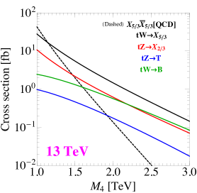
(a)  Partially composite $t_{R}^{\rm(P)}$ scenario.

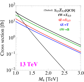
(b)  Fully composite $t_{R}^{\rm(F)}$ scenario.

Figure 2: The production cross sections of quartet top partners at the 13 TeV LHC. The parameters are chosen as $f=1$ TeV, $y_{L}=1$ and $c_{2}=1$ (for fully composite $t_{R}^{\rm(F)}$ only), while $y_{R}$ in partially composite $t_{R}^{\rm(P)}$ models and $y_{2L}$ in fully composite $t_{R}^{\rm(F)}$ models are determined by the top quark mass $M_{t}=150$ GeV (see Eq. (66) and Eq. (69)).

The production of fermion resonances can be categorized into QCD pair production and electroweak single production processes (see Ref. De Simone et al. (2013) for detail). The QCD production rate depends only on the mass of top partners. Since two heavy fermions are produced, the rate drops rapidly when the resonance’s mass increases because of the PDF suppression. In contrast, the single production channels typically have larger rates in the high mass region, thus it can play an important role in the search for heavier resonance Willenbrock and Dicus (1986); De Simone et al. (2013); Li et al. (2013); Aguilar-Saavedra et al. (2013); Mrazek and Wulzer (2010); Azatov et al. (2014); Backović et al. (2015a); Matsedonskyi et al. (2014); Backovic et al. (2016); Gripaios et al. (2014). This effect can be clearly seen from the Fig. 2, where we have plotted the cross sections for the resonances in the quartet at the 13 TeV LHC as functions of the Lagrangian parameter $M_{\textbf{4}}$. For these plots, we have chosen the following parameters:

$$f=1\,\text{TeV},\quad y_{L}=1,\quad c_{2}=1~{}(\text{for $t_{R}^{\rm(F)}$ only}),$$ (16)

where the parameter $y_{R}$ or $y_{2L}$ is determined by the top mass requirement for the partially composite $t_{R}^{\rm(P)}$ in Eq. (66) (the “P${}_{\textbf{4}}$ scenario”) or for the fully composite $t_{R}^{\rm(F)}$ in Eq. (69) (the “F${}_{\textbf{4}}$ scenario”), respectively. For the single production, we have combined the contribution of the top parters and their anti-particles. For example, for the charge-$5/3$ resonance $X_{5/3}$ in the quartet case, the $tW$ fusion process is defined as

$$\sigma(tW\to X_{5/3})\equiv\sigma(pp\to X_{5/3}\bar{t}q+\bar{X}_{5/3}tq).$$ (17)

The $tW\to B$ and $tZ\to T,~{}X_{2/3}$ processes are defined in a similar way. Figure 2 shows that, for both P${}_{\textbf{4}}$ and F${}_{\textbf{4}}$ scenarios, $tW\to X_{5/3}$ has the largest production rate among the 4 single production channels of the quartet fermionic resonances, and it dominates over the QCD pair production channel for $M_{\textbf{4}}\gtrsim 1$ TeV. Although the $tW\to X_{5/3}$ rates of those two scenarios are similar under our parameter choice, the rate of $tW\to B$ channel in P${}_{\textbf{4}}$ scenario is less than that in F${}_{\textbf{4}}$ scenario. This is because the former is from the composite-elementary Yukawa interaction $-y_{R}\bar{B}_{L}\phi^{-}t_{R}^{\rm(P)}$ (see Eq. (65)) and proportional to $c_{\theta_{L}}^{2}$, while the latter is mainly controlled by the strong dynamics term $-(\sqrt{2}c_{2}/f)\bar{B}_{R}\gamma^{\mu}t_{R}^{\rm(F)}i\partial_{\mu}\phi^{-}$ (see Eq. (68)) without such suppression. As $c_{\theta_{L}}$ will increase with $M_{\textbf{4}}$, we see the values of the two green lines in Fig. 2(a) and Fig. 2(b) become similar at large $M_{\textbf{4}}$. By naively using the Goldstone equivalence theorem, we expect

$$\sigma(tW\to X_{5/3})\approx\sigma(tW\to B)>\sigma(tZ\to T)\approx\sigma(tZ\to X_{2/3}),$$ (18)

if $y_{L}f/M_{\textbf{4}}\ll 1$ and the mass splittings of the top partners become negligible. From the figures we find that in the F${}_{\textbf{4}}$ scenario it is indeed the case, but in the P${}_{\textbf{4}}$ scenario it is not. The reasons is that in the P${}_{\textbf{4}}$ scenario, large $M_{\textbf{4}}$ requires large $y_{R}$ to correctly reproduce the mass of the top quark (see Eq. (66)), which results in a large mixing between the $T$ and $X_{2/3}$ resonances as shown in Eq. (67). Hence the naive estimate in Eq. (18) does not hold. We emphasize that the single production rates are more model-dependent. For example, the $tZ/W$ fusion rates in P${}_{\textbf{4}}$ scenario increase when $y_{L}$ decreases. This is because the constraint from observed top quark mass requires a larger $y_{R}$ as $y_{L}$ decreases, while the fusion rates are proportional to $(y_{R})^{2}$. But in the F${}_{\textbf{4}}$ scenario, the cross sections are rather insensitive to $y_{L}$, since they are mainly determined by the $c_{2}$ term.

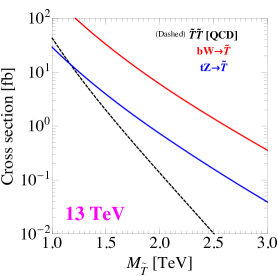
(a)  Partially composite $t_{R}^{\rm(P)}$ scenario.

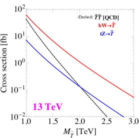
(b)  Fully composite $t_{R}^{\rm(F)}$ scenario.

Figure 3: The production cross sections of singlet top partners at the 13 TeV LHC. The parameters used in making these plots are $f=1$ TeV, $y_{L}=1.5~{}(1)$ for LP(F)${}_{\textbf{1}}$, while $y_{R}$, $y_{2L}$ are determined by the top quark mass $M_{t}=150$ GeV (see Eq. (66) and Eq. (69)). Note that $bW\rightarrow\widetilde{T}$ process is calculated using bottom PDF.

Similar to the quartet case, the single production mechanism of the singlet top partner $\widetilde{T}$ dominates over the QCD pair production if it is heavier than $\mathcal{O}(1)$ TeV, as shown in Fig. 3. Besides the $tZ\to\widetilde{T}$ fusion, the singlet can also be produced by $bW$ fusion:

$$\sigma(bW\to\widetilde{T})\equiv\sigma(pp\to\widetilde{T}q+\overline{\widetilde{T}}q).$$ (19)

In fact, the cross section of this channel is about an order of magnitude larger than the $tZ$ fusion due to the large bottom PDF, as can be seen from the red solid lines in Fig. 3. Note that for the partially composite $t_{R}^{\rm(P)}$ scenario, we have chosen a somewhat larger value $y_{L}=1.5$ in order to correctly reproduce the mass of the top quark in Eq. (87).

II.2.2 Decay of the composite resonances

Let’s now turn to the decay of the vector resonances . The decay branching ratios into different final states are determined by both the kinematics and the sizes of the couplings between the vector resonances and the final state particles.

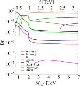
(a)  The branching ratios of $\rho_{L}^{+}$ in LP${}_{\textbf{4}}$.

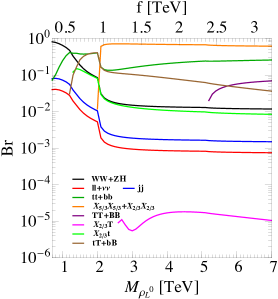
(b)  The branching ratios of $\rho_{L}^{0}$ in LP${}_{\textbf{4}}$.

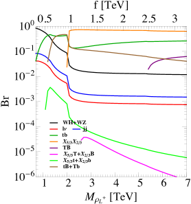
(c)  The branching ratios of $\rho_{L}^{+}$ in LF${}_{\textbf{4}}$.

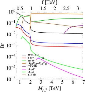
(d)  The branching ratios of $\rho_{L}^{0}$ in LF${}_{\textbf{4}}$.

Figure 4: The decay branching ratios of the $\rho_{L}^{\pm,0}$ resonances. The parameters are $g_{\rho_{L}}=3$, $a_{\rho_{L}}^{2}=1/2$, $M_{\textbf{4}}=1$ TeV, $y_{L}=1$ and $c_{1}=1$. For LF${}_{\textbf{4}}$ there is an additional parameter $c_{2}=1$.

Let’s start from the $\rho_{L}(\textbf{3},\textbf{1})$ resonances in models LP${}_{\textbf{4}}$ and LF${}_{\textbf{4}}$. In Fig. 4, we have plotted the decay branching ratios of $\rho_{L}^{\pm,0}$ as functions of $M_{\rho_{L}^{\pm,0}}$, choosing the following parameters:

$$g_{\rho_{L}}=3,\quad a_{\rho_{L}}^{2}=\frac{1}{2},\quad M_{\textbf{4}}=1~{}{\rm TeV},\quad y_{L}=1,\quad c_{1}=1,\quad c_{2}=1~{}\text{(for LF${}_{\textbf{4}}$ only).}$$ (20)

The parameter $f$ is determined by Eq. (62) and the parameters $y_{R}$ (LP${}_{\textbf{4}}$), $y_{2L}$ (LF${}_{\textbf{4}}$) are fixed by reproducing the observed top quark running mass $M_{t}=150~{}\text{GeV}$ at the TeV scale. Several comments are in order. In the low mass region $M_{\rho_{L}}<M_{\textbf{4}}$, $\rho_{L}$ can only decay into SM final states. Since we are interested in the mass region $M_{\rho}\gg M_{W,Z,h}$, we can neglect all the SM masses. Hence, the decaying branching ratios are completely determined by the couplings among $\rho_{L}$ and SM particles. As discussed above, only $\rho_{L}V_{L}V_{L}(h)$ $(V=W,Z)$ couplings belong to the first class and are enhanced by the strong coupling $g_{\rho_{L}}$. Besides this, there are $\rho_{L}\bar{q}_{L}q_{L}$ couplings, where $q_{L}$ are third generation left-handed quarks. They are of $\mathcal{O}(g_{\rho_{L}}s_{\theta_{L}}^{2})$ and can be relevant for the moderate size of $s_{\theta_{L}}$. Therefore, the dominant decay channels for this mass region are

$$\rho_{L}^{+}\rightarrow W^{+}Z,~{}W^{+}h,~{}t\bar{b};\quad\rho_{L}^{0}\rightarrow W^{+}W^{-},~{}Zh,~{}t\bar{t},~{}b\bar{b},$$ (21)

as shown in Fig. 4. There are no significant differences between the two models in this kinematical region. From the Goldstone equivalence theorem, the decay branching ratio of $\rho_{L}^{+}$ into $W^{+}Z$ is the same as $W^{+}h$ in the limit of $M_{\rho_{L}}\gg M_{W,Z,h}$ (see Eq. (8)). We only plot the sum of the two channels in Fig. 4. The same argument applied to the $W^{+}W^{-}$, $Zh$ decay channels of $\rho_{L}^{0}$. We also notice that for the SM light fermion channels, we have the accidental relations $\text{Br}(\rho_{L}^{+}\rightarrow jj)=2\times\text{Br}(\rho_{L}^{+}\rightarrow\ell^{+}\nu_{\ell})$ and $\text{Br}(\rho_{L}^{0}\rightarrow jj)=2\times\text{Br}(\rho_{L}^{0}\rightarrow\ell^{+}\ell^{-}+\nu_{\ell}\bar{\nu}_{\ell})$ as illustrated by LABEL:Brooijmans:2014eja,Greco:2014aza.

For the intermediate mass region, i.e. $M_{\textbf{4}}<M_{\rho_{L}}<2M_{\textbf{4}}$, the decay channels with one third generation quark and one top partner (the “heavy-light” channels) are open kinematically. For the charged resonance $\rho_{L}^{+}$, we have plotted the sum of branching ratios of the decay channels $t\bar{B}$ and $T\bar{b}$ and the sum of the decay channels $X_{5/3}\bar{t}$ and $X_{2/3}\bar{b}$. For the neutral resonances $\rho_{L}^{0}$, we have combined the channels $t\bar{T}$ and $b\bar{B}$ and their charge conjugate processes. Let’s start the discussion from the model LP${}_{\textbf{4}}$. The branching ratios of such channels grow quickly once they are kinematically open. This rapid increase is due to the strong coupling enhancement. At the same time, there is also a difference between the $t\bar{B}+T\bar{b}$ channels and the $X_{5/3}\bar{t}+X_{2/3}\bar{b}$ channels. The branching ratio for the former increases as $M_{\rho_{L}^{+}}$ becomes larger, while the branching ratio of the latter increases at the beginning then decreases as the mass of $\rho_{L}^{+}$ increase. We first note that the couplings $\rho_{L}^{+}X_{5/3}\bar{t}$, $\rho_{L}^{+}X_{2/3}\bar{b}$ are suppressed by the fine-tuning parameter $\xi=v^{2}/f^{2}$ (see Table 2). Since $g_{\rho_{L}}$ and $a_{\rho_{L}}$ are fixed, increasing mass $M_{\rho_{L}^{+}}$ will result in an increasing of the decay constant $f$ and a smaller $\xi$ parameter. The same behavior is also observed in the neutral resonance $\rho_{L}^{0}$ decay channels of $t\bar{T}+b\bar{B}$ and $X_{2/3}\bar{t}$ and their charge conjugates due to similar reasons. There is a difference here between the two models LP(F)${}_{\textbf{4}}$. For the partially composite $t_{R}^{\rm(P)}$ scenario, the decay channels $\rho_{L}^{+}\rightarrow X_{5/3}\bar{t}+X_{2/3}\bar{b}$ and $\rho_{L}^{0}\rightarrow X_{2/3}\bar{t}+\bar{X}_{2/3}t$ can become sizable $\sim 10\%$. However, for the fully composite $t_{R}^{\rm(F)}$, their branching ratios are below $1\%$. This is due to the fact that the couplings $\rho_{L}^{+}\bar{X}_{5/3R}t_{R}$, $\rho_{L}^{0}\bar{X}_{2/3R}t_{R}$ arise from $\mathcal{O}(\sqrt{\xi})$ in model LP${}_{\textbf{4}}$ and $\mathcal{O}(\xi)$ in model LF${}_{\textbf{4}}$, as can be seen clearly from Table 2 and Table 3. We also notice that $\rho_{L}^{+}\rightarrow t\bar{b}$, $\rho_{L}^{0}\rightarrow t\bar{t}+b\bar{b}$ decay channels are always sizable even in the intermediate mass region and the high mass region $M_{\rho_{L}}>2M_{\textbf{4}}$. This is due to the fact that we are fixing $y_{L}$ and $M_{\textbf{4}}$. Hence, increasing $M_{\rho_{L}}$ will also increase $f$. As a result, the left-handed mixing angle $s_{\theta_{L}}$ becomes larger. The branching ratio ranges from $20\%$ to $40\%$ in the intermediate mass region and above $10\%$ in the high mass region.

For the mass region of $M_{\rho_{L}}>2M_{\textbf{4}}$, the pure strong dynamics channels are kinematically allowed. Since their couplings are of $\mathcal{O}(g_{\rho})$ and we expect that they will dominate. Among those channels, the $\rho_{L}^{+}\to X_{5/3}\bar{X}_{2/3}$ channel has the largest branching ratios (above $60\%$), because they are the first and second lightest top partners. Note that the decaying channel into $T\bar{B}$ opens very slowly. In the parameter space under consideration, its branching ratio is always below $10\%$ and smaller than those of the decay channels $t\bar{b}$ and $t\bar{B}+T\bar{b}$. This behavior is due to the particular choice of our parameters in Eq. (20). In particular, the masses of $T,B$ are roughly given by

$$M_{T,B}\sim\sqrt{M_{\textbf{4}}^{2}+y_{L}^{2}M_{\rho_{L}}^{2}/(a_{\rho_{L}}^{2}g_{\rho_{L}}^{2})}\sim\sqrt{M_{\textbf{4}}^{2}+2M_{\rho_{L}}^{2}/9}.$$ (22)

Even for large $M_{\rho_{L}}$, the masses of $T,B$ are $\sim 0.47\times M_{\rho_{L}}$ and the decay into $T\bar{B}$ suffers from phase space suppression. We also expect that other choices of the parameters (for example smaller value of $y_{L}$) will make this channel more relevant. Things are similar in the case of $\rho_{L}^{0}$, where the decay channels into $\bar{X}_{5/3}X_{5/3}$, $\bar{X}_{2/3}X_{2/3}$ are dominant ($>60\%$) and $\bar{T}T+\bar{B}B$ decaying channels are below 10$\%$.

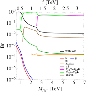
(a)  The branching ratios of $\rho_{R}^{+}$ in RP${}_{\textbf{4}}$.

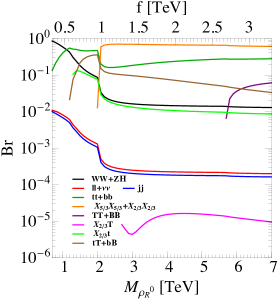
(b)  The branching ratios of $\rho_{R}^{0}$ in RP${}_{\textbf{4}}$.

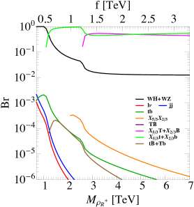
(c)  The branching ratios of $\rho_{R}^{+}$ in RF${}_{\textbf{4}}$.

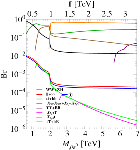
(d)  The branching ratios of $\rho_{R}^{0}$ in RF${}_{\textbf{4}}$.

Figure 5: The decay branching ratios of the $\rho_{R}^{\pm,0}$ resonances. The parameters are $g_{\rho_{R}}=3$, $a_{\rho_{R}}^{2}=1/2$, $M_{\textbf{4}}=1$ TeV, $y_{L}=1$ and $c_{1}=1$. For RF${}_{\textbf{4}}$ there is an additional parameter $c_{2}=1$. The $\text{Br}(T\bar{B})$ in subfigures (a) and (c) are less than $10^{-7}$, thus not shown in the figures.

Next we turn to the $(\textbf{1},\textbf{3})$ resonances $\rho_{R}^{\pm,0}$. The benchmark point is the same as that in the $\rho_{L}^{\pm,0}$ case, with the replacement $\rho_{L}\to\rho_{R}$. Unlike $\rho_{L}^{+}$, the $\rho_{R}^{+}$ does not mix with SM gauge bosons before EWSB because of its quantum number. Consequently, its decay branching ratios to SM light fermions are tiny. For example, it is less than $10^{-3}$ for the parameter space shown in Fig. 5(a) and 5(c). The decaying branching ratio into $t\bar{b}$ is also suppressed because the corresponding coupling arises after EWSB and is of order $\mathcal{O}(g_{\rho_{R}}\xi)$. As a consequence, the $\rho_{R}^{+}$ mainly decays into di-boson channels $W^{+}h+W^{+}Z$. In the intermediate mass region, the decaying into $X_{5/3}\bar{t}+X_{2/3}\bar{b}$ channels dominate over all the other channels with branching ratio larger than $90\%$ in both model LP${}_{\textbf{4}}$ and LF${}_{\textbf{4}}$, as their left-handed couplings arise before EWSB. The decay channels into $t\bar{B}+T\bar{b}$ are very small ($2\%-4\%$) for model LP${}_{\textbf{4}}$ and below $10^{-3}$ for model LF${}_{\textbf{4}}$. In the high-mass region, the dominant decaying channels are $X_{5/3}\bar{T}+X_{2/3}\bar{B}$ and $X_{5/3}\bar{t}+X_{2/3}\bar{b}$ with similar branching ratios. It is interesting to see that the heavy-light decay channel is still sizable in the high-mass region, as the mixing angle $s_{\theta_{L}}$ becomes larger for larger $\rho_{R}^{+}$ mass and the mass of $T$, $B$ increase with $M_{\rho_{R}}$ as discussed before. The neutral resonance $\rho_{R}^{0}$ mixes with the SM Hypercharge gauge boson before EWSB, resulting in the relation $\text{Br}(jj)=22/27\times\text{Br}(\ell^{+}\ell^{-}+\nu_{\ell}\bar{\nu}_{\ell})$ Brooijmans et al. (2014), as shown in Fig. 5(b) and 5(d). The branching ratios of the other decay channels of $\rho_{R}^{0}$ are very similar to those of $\rho_{L}^{0}$, and we will not discuss them further.

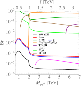
(a)  The branching ratios of $\rho_{X}^{0}$ in XP${}_{\textbf{4}}$.

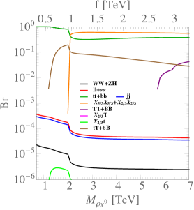
(b)  The branching ratios of $\rho_{X}^{0}$ in XF${}_{\textbf{4}}$.

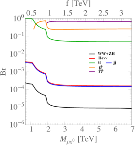
(c)  The branching ratios of $\rho_{X}^{0}$ in XP${}_{\textbf{1}}$.

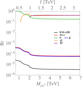
(d)  The branching ratios of $\rho_{X}^{0}$ in XF${}_{\textbf{1}}$.

Figure 6: The decay branching ratios of the $\rho_{X}^{0}$ resonances. The parameters are chosen as $g_{\rho_{X}}=3$, $a_{\rho_{X}}^{2}=1/2$, $M_{\textbf{4},\textbf{1}}=1$ TeV and $c_{1}=1$. For the XP${}_{\textbf{1}}$ model we have chosen $y_{L}=1.5$, while for other three models we set $y_{L}=1$. For the XF${}_{\textbf{4}}$ model, we set $c^{\prime}_{1}=1$, and for XF${}_{\textbf{1}}$, we set $c^{\prime}_{1}=c^{\prime\prime}_{1}=1$.

Finally, we study the $(\textbf{1},\textbf{1})$ resonance $\rho_{X}^{0}$. As an $SO(4)$ singlet, the $\rho_{X}^{0}$ can couple either to quartet $\Psi_{\textbf{4}}$ or to the singlet $\Psi_{\textbf{1}}$, and the corresponding models are XP(F)${}_{\textbf{4}}$ and XP(F)${}_{\textbf{1}}$, respectively. In our plots, the parameters chosen are very similar to the benchmark point of $\rho_{L}^{\pm,0}$, except for XP${}_{\textbf{4}}$ where we choose $y_{L}=1.5$. For the XF${}_{\textbf{4},\textbf{1}}$ model, there is another parameter $c_{1}^{\prime}$ describing the direct interaction between the fully composite $t_{R}^{\rm(F)}$ and the $\rho_{X}^{0}$ resonance, and it is set to be 1. For the XF${}_{\textbf{1}}$ model, we further set $c^{\prime\prime}_{1}$ (the parameter describing the interaction between $t_{R}^{\rm(F)}$ and the $\rho_{X}^{0}$, $\Psi_{\textbf{1}}$ resonances) to be 1. Since the $U(1)_{X}$ has no direct connection to the dynamical symmetry breaking $SO(5)\to SO(4)$, its corresponding spin-1 resonance $\rho_{X}^{0}$ does not couple to the Goldstone boson $H$ before EWSB. Consequently, the decaying branching ratios into SM di-bosons $W^{+}W^{-}+Zh$ are very small ($<10^{-4}$). The di-fermion decay channels of XP(F)${}_{\textbf{4}}$ are very analogous to those of $\rho_{R}^{0}$ in RP(F)${}_{\textbf{4}}$. The most relevant channels are $\rho_{X}^{0}\rightarrow t\bar{t}+b\bar{b}$ in the low-mass region, $\rho_{X}^{0}\rightarrow t\bar{T}+\bar{t}T+b\bar{B}+\bar{b}B$ in the intermediate mass region, and $\rho_{X}^{0}\rightarrow\bar{X}_{5/3}X_{5/3}+\bar{X}_{2/3}X_{2/3}$ in the high-mass region . In models with singlet top partner XP(F)${}_{\textbf{1}}$, since the $b$ quark does not mix with the resonance, we classify as one of the “SM light fermions”. Therefore, we have $\text{Br}(jj)=\text{Br}(\ell^{+}\ell^{-}+\nu_{\ell}\bar{\nu}_{\ell})$, as shown in the bottom panel of Fig. 6. In model XP${}_{\textbf{1}}$, the dominant decaying channels are $\rho_{X}^{0}\rightarrow t\bar{t}$ in the low-mass region, $\rho_{X}^{0}\rightarrow\bar{t}\widetilde{T}+\overline{\widetilde{T}}t$ ($\sim$ 70%) in the intermediate mass region and $\rho_{X}^{0}\rightarrow\overline{\widetilde{T}}\widetilde{T}(\sim 70\%)$ in the high mass region. The situation is similar in the model XF${}_{\textbf{1}}$ except that in the high-mass region, the $\rho_{X}^{0}\rightarrow t\bar{t}$ and $\rho_{X}^{0}\rightarrow\bar{t}\widetilde{T}+\overline{\widetilde{T}}t$ decaying channels are also relevant. Their branching ratios are around $20\%$ and $40\%$, respectively.

III The present limits and prospective reaches at the LHC

In this section, we present the current limits and prospective reaches for the simplified models at the LHC.

III.1 Making projections

For the projections at the high luminosity or high energy LHC, we extrapolate from the current LHC searches using a similar method as in LABEL:Thamm:2015zwa. We described the method in detail in Appendix E.

There have been a number of searches for beyond the SM (BSM) resonances at the LHC, providing constraints to the composite Higgs models. To use a more generic and uniform notation in describing the searches, we denote the spin-1 resonances as $\rho$ and the spin-$1/2$ resonances as $F_{Q}$, where $Q$ is the electric charge. The results at the 13 TeV LHC can be classified into two main groups. The first group is the Drell-Yan production and two-body decay of $\rho$, its various final states can be summarized as follows,

1. SM di-fermion final states, including di-lepton, di-jet, and the third generation quark-involved channels. We list the relevant measurements in Table 5.

   Channel	Collaboration and corresponding integrated luminosity
   $q\bar{q}\to\rho^{0}\to\ell^{+}\ell^{-}$	ATLAS at 36 fb-1 Aaboud et al. (2017a); CMS at 77.3 fb-1 (for $e$ channel) and 36.3 fb-1 (for $\mu$ channel) CMS (2018a).
   $q\bar{q}^{\prime}\to\rho^{\pm}\to\ell^{+}\nu/\ell^{-}\bar{\nu}$	ATLAS at 79.8 fb-1 ATL (2018b); CMS at 35.9 fb-1 Sirunyan et al. (2018b); CMS (2018b).
   $q\bar{q}^{(\prime)}\to\rho^{\pm,0}\to jj$	ATLAS at 37 fb-1 Aaboud et al. (2017b); CMS at 77.8 fb-1 CMS (2018c).
   $q\bar{q}^{(\prime)}\to\rho^{\pm,0}\to jj$ (with $b$-tagging)	ATLAS at 36.1 fb-1 Aaboud et al. (2018a).
   $q\bar{q}\to\rho^{0}\to t\bar{t}$	ATLAS at 36.1 fb-1 Aaboud et al. (2018b); CMS at 35.9 fb-1 Sirunyan et al. (2018c).
   $q\bar{q}^{\prime}\to\rho^{\pm}\to t\bar{b}/\bar{t}b$	ATLAS at 36.1 fb-1 Aaboud et al. (2018c, 2019); CMS at 35.9 fb-1 Sirunyan et al. (2018d).

   Table 5: The present searches for BSM spin-1 resonances in di-fermion final states at the 13 TeV LHC.

2. SM di-boson final states. The topology is $q\bar{q}^{(\prime)}\to\rho^{\pm,0}\to W^{\pm}Z/W^{+}W^{-}/W^{\pm}h/Zh$, and different final states are summarized in Table 6. Note that we have no $hh$ or $ZZ$ final states from the decay of spin-1 resonances in composite Higgs models .

   	$V\to qq$	$W\to\ell\nu$ or $Z\to\ell\ell/\nu\bar{\nu}$
   $V\to qq$	ATLAS at 79.8 fb-1 ATL (2018a); CMS at 35.9 fb-1 Sirunyan et al. (2018e).	$-$
   $W\to\ell\nu$	ATLAS at 36.1 fb-1 Aaboud et al. (2018d); CMS at 35.9 fb-1 Sirunyan et al. (2018f);	ATLAS at 36.1 fb-1 Aaboud et al. (2018e).
   $Z\to\ell\ell$	ATLAS at 36.1 fb-1 Aaboud et al. (2018f); CMS at 35.9 fb-1 Sirunyan et al. (2018g);	ATLAS at 36.1 fb-1 Aaboud et al. (2018g).
   $Z\to\nu\nu$	ATLAS at 36.1 fb-1 Aaboud et al. (2018f); CMS at 35.9 fb-1 Sirunyan et al. (2018h).	$-$
   $h\to bb$	ATLAS at 36.1 fb-1 Aaboud et al. (2017c); CMS at 35.9 fb-1 Sirunyan et al. (2017a);	ATLAS at 36.1 fb-1 Aaboud et al. (2018h); CMS at 35.9 fb-1 Sirunyan et al. (2018i).
   $h\to\tau\tau$	CMS at 35.9 fb-1 Sirunyan et al. (2018j).	$-$

   Table 6: The searches for BSM spin-1 resonances in di-boson final states at the 13 TeV LHC, where $V$ denotes $W^{\pm}$, $Z$. The search in Ref. Aaboud et al. (2018g) is also sensitive to the VBF production of $\rho^{\pm}$, but the constraint is quite weak ($\lesssim 1$ TeV). For a summary of the di-boson results from ATLAS at $\sim 36~{}{\rm fb}^{-1}$, we refer the readers to Ref. Aaboud et al. (2018i).

3. The $tF_{Q}$ final state, i.e. the heavy resonance-SM fermion channel with one top quark and one top partner. The newest result is $q\bar{q}\to\rho^{0}\to t\bar{F}_{2/3}\to t\bar{t}Z$, measured by CMS at 35.9 fb^-1 Sirunyan et al. (2018k); CMS (2018d). Hereafter, for simplicity the charge conjugate of the particle decay final state is always implied; for example, $t\bar{F}_{2/3}$ denotes both $t\bar{F}_{2/3}$ and $\bar{t}F_{2/3}$.

The second group of limits are from the search of the fermionic resonances $F_{Q}$. Their production mechanisms can be categorized into QCD pair production and single production processes. For the QCD pair production, $pp\to F_{Q}\bar{F}_{Q}$, the experimental collaborations have searched for resonances with different charges in various decay channels. The results relevant to our models are the searches for $F_{2/3}\to tZ/th/bW$, $F_{-1/3}\to tW^{-}$ and $F_{5/3}\to tW^{+}$ in various final states by the ATLAS and CMS collaborations at an integrated luminosities around 36 fb^-1 Aaboud et al. (2017d, 2018j, e); Sirunyan et al. (2018l); Aaboud et al. (2018k); CMS (2017); Sirunyan et al. (2018a); ATL (2018c); Aaboud et al. (2018l); Sirunyan et al. (2018m); Aaboud et al. (2018m, n). A summary of the QCD pair produced top partner searches by the ATLAS Collaboration can be found in Ref. Aaboud et al. (2018o).

In addition, there have been searches for singly produced top partners. Such channels typically have larger rates than the QCD pair production. However, they are also more model-dependent. Currently, the $bW\to F_{2/3}\to bW$ channel is explored by ATLAS at 3.2 fb^-1 ATL (2016) and CMS at 2.3 fb^-1 Sirunyan et al. (2017b); while the singly produced $F_{2/3}\to tZ$ channel has been searched with 36 fb^-1 by CMS Sirunyan et al. (2018k) ($tZ$ fusion) and ATLAS Aaboud et al. (2018l) ($bW$ fusion). The $tW$ fusion production of $F_{5/3}$ (or $F_{-1/3}$) has been searched by CMS at 35.9 fb^-1 Sirunyan et al. (2018n) and by ATLAS at 36.1 fb^-1 Aaboud et al. (2018m).

For the new channels we propose in this paper, especially the cascade decays of the $\rho$ resonances to the heavy fermionic resonances, there have been no dedicated searches. We estimate their exclusion by recasting existing searches using the SSDL final states $\ell^{\pm}\ell^{\pm}{\rm+jets}$. In Table 7, we have listed the existing searches for the resonances at the LHC using $\ell^{\pm}\ell^{\pm}{\rm+jets}$ final state. The upper limit on the cross section of the highest mass points considered in the searches and the corresponding number of events before any kinematic cuts are reported in the table. Motivated by these results, we assume that a limit can be set for $N(\ell^{\pm}\ell^{\pm}+{\rm jets})=20$ before any kinematical cuts.

Experimental searches	Cross section upper limit of the tail	Event number before cut
CMS at 35.9 fb-1 CMS (2017)	$\sigma(pp\to X_{5/3}\bar{X}_{5/3}\to tW\bar{t}W)=16$ fb at 1.5 TeV	$N(\ell^{\pm}\ell^{\pm}+{\rm jets})=23$
CMS at 35.9 fb-1 Sirunyan et al. (2017c)	$\sigma(pp\to t\bar{t},tW,tq+X){\rm Br}(X\to t\bar{t})=30$ fb at 0.55 TeV X denotes a new scalar or pseudo-scalaer	$N(\ell^{\pm}\ell^{\pm}+{\rm jets})=42$
ATLAS at 36.1 fb-1 Aaboud et al. (2017f)	$\sigma(pp\to\widetilde{b}_{R}\widetilde{b}_{R}\to\bar{t}\bar{s}\bar{t}\bar{s})=14$ fb at 1.6 TeV $\widetilde{b}_{R}^{\dagger}\widetilde{b}_{R}^{\dagger}$ is not included because PDF $f_{\bar{d}}\ll f_{d}$.	$N(\ell^{-}\ell^{-}+{\rm jets})=20$

Table 7: The experimental results of the SSDL final states at the 13 TeV LHC.

Next, we present the results for models LP(F)${}_{\textbf{4}}$, RP(F)${}_{\textbf{4}}$, XP(F)${}_{\textbf{4}}$ and XP(F)${}_{\textbf{1}}$ in subsequent subsections.

III.2 The results of LP${}_{\textbf{4}}$ and LF${}_{\textbf{4}}$

In this subsection, we investigate the current limits and prospective reaches on the models LP(F)${}_{\textbf{4}}$ at the 13 TeV LHC. In the Lagrangian of LP${}_{\textbf{4}}$ in Eq. (52), there are 10 parameters:

$$\{g_{2},\;g_{1},\;v,\;g_{\rho_{L}},\;a_{\rho_{L}},\;f,\;M_{\textbf{4}},\;y_{L},\;y_{R},\;c_{1}\}.$$

The electroweak input parameters $\{\alpha,M_{Z},G_{F},M_{t}\}$ provide 4 constraints, leaving us 6 free parameters, which we have chosen to be $\{g_{\rho_{L}},a_{\rho_{L}},M_{\rho_{L}^{0}},M_{\textbf{4}},y_{L},c_{1}\}$. Because $M_{\rho_{L}^{0}}$ is nearly degenerate with $M_{\rho_{L}^{\pm}}$, we denote them with the same variable $M_{\rho_{L}}$. Note that the Lagrangian mass $M_{\textbf{4}}$ is also the exact physical mass of $X_{5/3}$ after EWSB, since none of the SM particles can mix with it. For LF${}_{\textbf{4}}$, the situation is almost the same, expect there is an additional $\mathcal{O}(1)$ strong dynamics parameter $c_{2}$. To better demonstrate the interplay of the spin-1 and spin-$1/2$ resonances, we scan $(M_{\rho_{L}},M_{X_{5/3}})$ while fixing the other parameters to a benchmark point

$$g_{\rho_{L}}=3,\quad a_{\rho_{L}}^{2}=\frac{1}{2},\quad y_{L}=1,\quad c_{1}=1,\quad c_{2}=1~{}(\text{for LF${}_{\textbf{4}}$ only}).$$ (23)

The results of LP${}_{\textbf{4}}$ and LF${}_{\textbf{4}}$ are shown in Fig. 7(a) and 7(b), respectively. Since $g_{\rho_{L}}$ is fixed, $f$ is determined by $M_{\rho_{L}}$, and we use its value to label the top horizontal axis.

We plot the existing bounds from LHC searches and their extrapolations at 300 (3000) fb^-1 in colored shaded regions. Besides the direct searches for resonances, the measurement of and $\xi$ parameter can provide an indirect constraint. Currently LHC results imply $\xi\lesssim 0.13$ Sanz and Setford (2018); de Blas et al. (2018), while the further constraints are expected to be as good as $0.066$ ($0.04$) with 300 (3000) fb^-1 of data CMS (2012); ATL (2013); Dawson et al. (2013). We also plot the constraints on $\xi$ in the figures as vertical black thin lines.

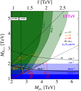
(a)  The results of LP${}_{\textbf{4}}$.

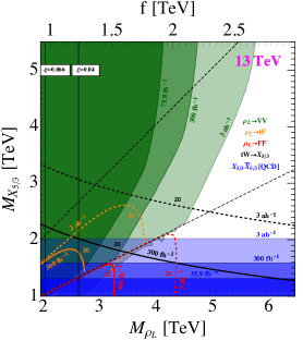
(b)  The results of LF${}_{\textbf{4}}$.

Figure 7: The current limits and prospective reaches on model LP${}_{\textbf{4}}$ (left plot) and model LF${}_{\textbf{4}}$ (right plot). The parameters are chosen as Eq. (23). The existing limits are shown as the darkest shaded regions, while the projections for 300 (3000) fb^-1 are plotted the lighter shaded regions. The production channels include Drell-Yan $\rho_{L}^{\pm,0}\to W^{\pm}Z/W^{+}W^{-}$ ATL (2018a) (denoted as $\rho_{L}\to VV$) and QCD pair production of $X_{5/3}\bar{X}_{5/3}$ Sirunyan et al. (2018a). The event number contours for $N(\ell^{\pm}\ell^{\pm}+\text{jets})=20$ are plotted in solid (dashed) lines for 300 (3000) fb^-1, to set a prospective limit for the proposed channels, including $\rho_{L}^{\pm}\to t\bar{B}/X_{5/3}\bar{t}$ (denoted as $\rho_{L}\to tF$), $\rho_{L}^{\pm,0}\to X_{5/3}\bar{X}_{2/3}/X_{5/3}\bar{X}_{5/3}$ (denoted as $\rho_{L}\to FF$) and $tW\to X_{5/3}$. See the main text for more details.

Putting all the constraints and projections together, we see that the future data at the LHC will explore the parameter space of LP(F)${}_{\textbf{4}}$ extensively . The constraints are similar in the two models LP(F)${}_{\textbf{4}}$ . For a relatively large value of $g_{\rho_{L}}$ (for example, $g_{\rho_{L}}=3$ in our benchmark point), the most sensitive channel in the $M_{\rho_{L}}<2M_{X_{5/3}}$ region is the $W^{\pm}Z/W^{+}W^{-}$ search with boosted di-jet channel performed by the ATLAS Collaboration with integrated luminosity $L=$ 79.8 fb^-1 in Ref. ATL (2018a). In such a mass region, the $\Gamma_{\rho_{L}}/M_{\rho_{L}}$ ratio is $\sim 0.8\%$ for our chosen parameters, thus the narrow width approximation works very well. If $g_{\rho_{L}}\lesssim 2$, the di-lepton $\ell^{+}\ell^{-}$ channel by CMS with $L=77.3~{}{\rm fb}^{-1}(e^{+}e^{-})+36.3~{}{\rm fb}^{-1}(\mu^{+}\mu^{-})$ CMS (2018a) gives the strongest limit. Because of the large experimental uncertainty, the $\rho\to t\bar{t}$, $b\bar{b}$ and $t\bar{b}$ channels are not able to give competitive limits, although they have significant branching ratios. In Fig. 7, we only show the present limits and prospective reaches from ATLAS di-boson boosted jet channels in Ref. ATL (2018a). It is clear from the figure that the interactions with light top-partner has affected the phenomenology of $\rho_{L}$ significantly. In particular, the present bound is relaxed from 4.2 TeV to 2.6 TeV for our benchmark parameters in Eq. (23) as the mass of top partner changes from $M_{X_{5/3}}\gg M_{\rho_{L}}$ to $M_{\rho_{L}}\gtrsim 2M_{X_{5/3}}$. Once the decays into pair of top partners are kinematically open, the bound becomes very weak. At the same time, very light top partners have been excluded by the direct searches for the top partner.

In the mass region of $M_{X_{5/3}}<M_{\rho_{L}}\leqslant 2M_{X_{5/3}}$, the decays of $\rho_{L}$ into one top partner and one SM particles are kinematically allowed. The width of the $\rho_{L}$ resonance is enhanced by the existence of those new channels, but still within the narrow width range. For example, in our benchmark Eq. (23), $\Gamma_{\rho_{L}}/M_{\rho_{L}}$ is $4.8\%-1.2\%$ for $M_{X_{5/3}}=0.6\times M_{\rho_{L}}-0.9\times M_{\rho_{L}}$. The $t\bar{t}Z$ final state from the decay channel $\rho_{L}^{0}\to t\bar{T}$ has been studied both experimentally Sirunyan et al. (2018k); CMS (2016) and theoretically Backović et al. (2017), but current experimental results are still too weak to be visible in Fig. 7. The $\rho_{L}^{\pm}\to T\bar{b}\to t\bar{b}Z$ channel is studied phenomenologically in Ref. Vignaroli (2014). In this work, we propose that the $t\bar{t}W^{\pm}\to\ell^{\pm}\ell^{\pm}+{\rm jets}$ final state from $\rho_{L}^{\pm}\to t\bar{B}/t\bar{X}_{5/3}$ can also be a good channel to probe such a heavy-light decay. In Fig. 7, we have plotted the contours for the constant number ($=20$) of SSDL events summing all these decay channels at 300 fb^-1 and 3 ab^-1 LHC. These channels have sensitivity to the parameter space up to $M_{\rho_{L}}=3.8$ TeV at 3 ab^-1 LHC, but it still can’t compete with the di-boson jet searches. This is due to the fact that the branching ratios into the heavy-light channels are not significantly larger than the di-boson channel and the decaying branching ratios to the SSDL are very small. It is interesting to explore other more complicated final states like $1\ell+{\rm jets}$ and we leave this for future possible work.

In the mass region of $M_{\rho_{L}}>2M_{X_{5/3}}$, the spin-1 resonances will decay dominantly into pairs of top partners, as discussed in detail in Sec. II.2.2. We focus here on the decay channels resulting in the SSDL final states: $\rho_{L}^{\pm,0}\to X_{5/3}\bar{X}_{2/3}/X_{5/3}\bar{X}_{5/3}$ (see also Refs. Barducci and Delaunay (2016); Vignaroli (2014) for the study of these channels). We plot the contours with 20 SSDL events, summing over all the above decay channels for 300 fb^-1 and 3 ab^-1 LHC. The prospective for the cascade decay channels are very promising and comparable with direct searches for the pair produced $X_{5/3}$. If the top partner is around 1 TeV, these channels can be promising to discover the heavy spin-1 resonance . Note that in such region the $\Gamma_{\rho_{L}}/M_{\rho_{L}}$ can be large. For example, for our benchmark point Eq. (23), $\Gamma_{\rho_{L}}/M_{\rho_{L}}$ varies from 56% to 37% when $M_{X_{5/3}}$ varies from $0.1\times M_{\rho_{L}}$ to $0.4\times M_{\rho_{L}}$. It is interesting to study the effects of large decay width on the resonance searches and we leave this for a future work. Here we just estimate the bounds by an event-counting method based on the SSDL final state, which does not require the reconstruction of a resonance peak. We expect such an estimate has less dependence on the width of $\rho_{L}$.

We have shown the present bounds and the prospectives of the searches for QCD pair produced $X_{5/3}\bar{X}_{5/3}$ in the $1\ell+{\rm jets}$ final state by CMS Sirunyan et al. (2018a) . The single top partner production may play an important role in the relatively high top parter mass region as discussed in Sec. II.2.1. Currently, the $tZ\to T/X_{2/3}$ channel has been searched by CMS at 35.9 fb^-1 Sirunyan et al. (2018k), and the $tW\to X_{5/3}$ channel has been searched by CMS at 35.9 fb^-1 Sirunyan et al. (2018n) in $1\ell+{\rm jets}$ final state and by ATLAS at 36.1 fb^-1 Aaboud et al. (2018m) in SSDL final state. However, the mass reaches of all those searches are still too low to be visible in our figures. Instead, in Fig. 7 we present the contours with constant number of events (= 20) in the $tW\rightarrow X_{5/3}\rightarrow\ell^{\pm}\ell^{\pm}+{\rm jets}$ final states as a projection for the future run of the LHC. The reach in model LP${}_{\textbf{4}}$ range from 1.5 TeV to 2 TeV at the 300 fb^-1 LHC and from 2.3 TeV to 3.1 TeV at the 3 ab^-1 HL-LHC which is better than the QCD pair searches (1.3 TeV at 300 fb^-1 and 2.0 TeV at 3 ab^-1).

III.3 The results of RP${}_{\textbf{4}}$ and RF${}_{\textbf{4}}$

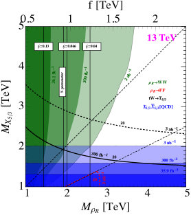
(a)  The results of RP${}_{\textbf{4}}$.

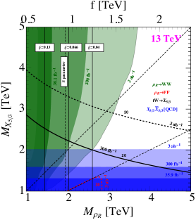
(b)  The results of RF${}_{\textbf{4}}$.

Figure 8: The current limits and prospective reach on model RP${}_{\textbf{4}}$ (left plot) and model RF${}_{\textbf{4}}$ (right plot). The parameters are chosen as Eq. (24). The existing limits from Drell-Yan $\rho_{R}^{0}\to W^{+}W^{-}$ Aaboud et al. (2018d) and $X_{5/3}\bar{X}_{5/3}$ [QCD] Sirunyan et al. (2018a) are shown as the darkest shaded regions, while the projections for 300 (3000) fb^-1 are shown as lighter shaded regions. The event number contours for $N(\ell^{\pm}\ell^{\pm}+\text{jets})=20$ are drawn in solid (dashed) lines for 300 (3000) fb^-1, as a prospective limit for the $\rho_{R}^{0}\to X_{5/3}\bar{X}_{5/3}$ (denoted as $\rho_{R}\to FF$) and the $tW\to X_{5/3}$ channels.

We now turn to discuss the models RP(F)${}_{\textbf{4}}$. Similar to the cases of LP(F)${}_{\textbf{4}}$, we have set the following parameters as

$$g_{\rho_{R}}=3,\quad a_{\rho_{R}}^{2}=\frac{1}{2},\quad y_{L}=1,\quad c_{1}=1,\quad c_{2}=1~{}\text{(for RF${}_{\textbf{4}}$ only)},$$ (24)

and scanned over $(M_{\rho_{R}},M_{X_{5/3}})$. The results are plotted in Fig. 8. The meanings of the shaded regions and contour lines are similar to those in Fig. 7. Note that we have started from $M_{\rho_{R}}$ from 1 TeV. Because the production cross sections of charged $\rho_{R}^{\pm}$ resonances are very small, we only use the searches for the Drell-Yan production of $\rho_{R}^{0}$ at the LHC. Similar to the search for the $\rho_{L}$ resonances, the di-boson channel provides the strongest constraints in the region of $M_{\rho_{R}}<2M_{\textbf{4}}$. Among the existing limits, we found that the diboson resonance searches by ATLAS in the semi-leptonic channel Aaboud et al. (2018d) and in the fully hadronic channel in ATL (2018a) give the strongest constraints, and their results are similar. Here we show the limits from results of LABEL:Aaboud:2017fgj. As expected, due to the smallness of hypercharge gauge coupling, the bound is weaker than the $\rho_{L}$ resonances. The present bound is around 1.6 TeV and will reach 3.8 TeV at the HL-LHC. In the mass region of $M_{X_{5/3}}<M_{\rho_{R}}\leqslant 2M_{X_{5/3}}$, the $\rho_{R}^{0}\to t\bar{X}_{2/3}\to t\bar{t}Z$ may be relevant, but the current search in Ref. Sirunyan et al. (2018k) is still not possible to put any relevant constraint in our parameter space. Thus, it is not shown in the figure. In the mass region of $M_{\rho_{R}}>2M_{X_{5/3}}$, the cascade decay channel $\rho_{R}^{0}\to X_{5/3}\bar{X}_{5/3}$ in the SSDL final state is not comparable with the searches for the QCD pair $X_{5/3}$ production, due to the smallness of the production cross section. We can also read from the figure that the electroweak precision $\hat{S}$-parameter measured by LEP Tanabashi et al. (2018) sets a strong constraint on the models with $\rho_{R}$, requiring $M_{\rho_{R}}\gtrsim 1.95$ TeV, which is heavier than current experimental reach. However, the reach of LHC with an integrated luminosity of 300 fb^-1 could surpass this constraint. The bounds for the top parters are the same as models LP(F)${}_{\textbf{4}}$ and not discussed here anymore.

III.4 The results of XP${}_{\textbf{4}}$ and XF${}_{\textbf{4}}$

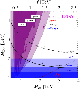
(a)  The results of XP${}_{\textbf{4}}$.

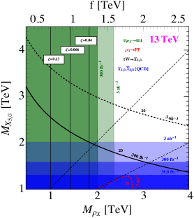
(b)  The results of XF${}_{\textbf{4}}$.

Figure 9: The current limits and prospective reach on model XP${}_{\textbf{4}}$ (left plot) and model XF${}_{\textbf{4}}$ (right plot). The parameters are chosen as Eq. (25). The existing limits and projections from $X_{5/3}\bar{X}_{5/3}$ [QCD] Sirunyan et al. (2018a) are plotted as shaded regions. The green regions come from $t\bar{t}\rho_{X}^{0}$ associated production, by the phenomenological study of Ref. Liu and Mahbubani (2016). The purple regions represent the limit from the $\ell^{+}\ell^{-}$ search CMS (2018a) and its extrapolations. The contours for $N(\ell^{\pm}\ell^{\pm}+\text{jets})=20$ are drawn with solid (dashed) lines for 300 (3000) fb^-1, as a prospective reach for the $\rho_{X}^{0}\to X_{5/3}\bar{X}_{5/3}$ (denoted as $\rho_{X}\to FF$) and the $tW\to X_{5/3}$ channels. See the text for more details.

We now turn to the models with a singlet vector resonance $\rho_{X}^{0}$. In this subsection we will discuss its interactions with the quartet top partner in models XP(F)${}_{\textbf{4}}$, while in the next subsection we will investigate its interactions with the singlet top partner XP(F)${}_{\textbf{1}}$. As discussed in LABEL:Greco:2014aza, $\rho_{X}$ only contributes to the $Y$-parameter of the electroweak precision test (see also Eq. (81)). Due to the $(g^{\prime}/g_{\rho_{X}})^{2}$ suppression, the indirect constraint on the $\rho_{X}$ is weak. As a result, $\rho_{X}$ could be very light especially in the case of large $g_{\rho_{X}}$. We choose the benchmark values for the parameters as

$$g_{\rho_{X}}=3,\quad a_{\rho_{X}}^{2}=\frac{1}{4},\quad y_{L}=1,\quad c_{1}=1,\quad c_{1}^{\prime}=c_{2}=1~{}\text{(for XF${}_{\textbf{4}}$ only)},$$ (25)

and scan over $(M_{\rho_{X}},M_{X_{5/3}})$ in Fig. 9. Note that we have chosen a slightly smaller value of $a_{\rho_{X}}$ in order to relax the bound from $\xi$ measurement. Here we can see a difference between the partially composite $t_{R}^{\rm(P)}$ and the fully composite $t_{R}^{\rm(F)}$ scenario. While the di-lepton channel CMS (2018a) can play an important role in model XP${}_{\textbf{4}}$ in the large $M_{X_{5/3}}$ region (i.e. $M_{X_{5/3}}>M_{\rho_{X}}$), it won’t put any significant constraint on the model XF${}_{\textbf{4}}$. This is due to the fact that the branching ratio of di-lepton in the model XP${}_{\textbf{4}}$ scales like $\left[g^{\prime}/(g_{\rho_{X}}s_{\theta_{L}})\right]^{4}$, while in model XF${}_{\textbf{4}}$, it scales like $(g^{\prime}/g_{\rho_{X}})^{4}$. As we fix $y_{L}$, larger value of $M_{X_{5/3}}$ will induce smaller value of $s_{\theta_{L}}$ and an enhancement of the di-lepton branching ratio in model XP${}_{\textbf{4}}$. Note that in the region $M_{\rho_{X}}\leqslant M_{X_{5/3}}$ where $\rho_{X}^{0}$ only decays to SM particles, the $t\bar{t}$ and $b\bar{b}$ channels dominate. The sensitivity in these channels at the 13 TeV LHC is roughly three order of magnitude worse than the di-lepton channel, assuming the same branching ratios. Thus they can only play a role in the large $g_{\rho_{X}}$ region. However, large $g_{\rho_{X}}$ will lead to small Drell-Yan production cross section and make $t\bar{t}$, $b\bar{b}$ channels not relevant in our parameter space. In contrast, the authors of Ref. Liu and Mahbubani (2016) have pointed out that the $pp\to t\bar{t}\rho_{X}^{0}\to t\bar{t}t\bar{t}$ channel with the SSDL final states can probe the fully composite $t_{R}^{\rm(F)}$ scenario very well, as the production cross section scales like $g^{2}_{\rho_{X}}$. In Fig. 9, we have reinterpreted the results of Ref. Liu and Mahbubani (2016) in our parameter space in model XF${}_{\textbf{4}}$. We see that $\rho_{X}^{0}$ with mass below 2 (2.4) TeV can be probed at 300 (3000) fb^-1 LHC with our choice of $g_{\rho_{X}}=3$ in model XF${}_{\textbf{4}}$. While for model XP${}_{\textbf{4}}$, the bound (not shown in the figure) is weaker ($\sim 1.0$ TeV at 3 ab^-1) due to the suppression of $\rho_{X}t\bar{t}$ couplings either by the $t_{L}-T_{L}$ mixing or the $B_{\mu}-\rho_{X\mu}$ mixing. We can also see that the limits from $t\bar{t}\rho_{X}$ channel become stronger in the low $M_{X_{5/3}}$ region in model XP${}_{\textbf{4}}$, as the left-handed top quark mixing angle $s_{\theta_{L}}$ becomes large. We also noticed that the cascade decays to top partner can barely play an important role, as the cross section of $\rho_{X}^{0}$ is small. The bounds on the quartet top partners are the same as models LP(F)${}_{\textbf{4}}$.

III.5 The results of XP${}_{\textbf{1}}$ and XF${}_{\textbf{1}}$

Finally we come to the models containing a singlet top partner, XP${}_{\textbf{1}}$ and XF${}_{\textbf{1}}$. While the scanning over $(M_{\rho_{X}},M_{\widetilde{T}})$, the other parameters are chosen as

$$g_{\rho_{X}}=3,\quad a_{\rho_{X}}^{2}=\frac{1}{4},\quad c_{1}=1,\quad y_{L}=1.5~{}(1.0)~{}\text{for XP${}_{\textbf{1}}$ (XF${}_{\textbf{1}}$)},\quad c_{1}^{\prime}=c_{1}^{\prime\prime}=1~{}(\text{XF${}_{\textbf{1}}$)}.$$ (26)

where we have chosen a slightly larger value of $y_{L}$ in model XP${}_{\textbf{1}}$ in order to reproduce the observed value of top quark mass. Note that in model XP${}_{\textbf{1}}$, the top quark mass is approximately given by Eq. (87)

$$M_{t}=\frac{y_{L}vs_{\theta_{R}}}{\sqrt{2}},$$

and the choice for $y_{L}$ in Eq. (26) has fixed $s_{\theta_{R}}\sim 0.6$. This means that the couplings of the interactions $\rho_{X}\bar{t}_{R}t_{R}$, $\rho_{X}\bar{t}_{R}\widetilde{T}_{R}$ are roughly constants with varying mass of the top partner (see Table 4). In both models, the Drell-Yan production of the $\rho_{X}$ can’t play an important role in our interested parameter space, because of the lack of the sensitivity to the dominant decay channel $t\bar{t}$ and the suppression of the decay branching ratio into the di-lepton final state.

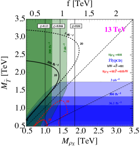
(a)  The results of XP${}_{\textbf{1}}$.

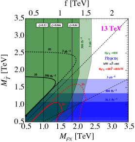
(b)  The results of XF${}_{\textbf{1}}$.

Figure 10: The current limits and prospective reach on model XP${}_{\textbf{1}}$ (left plot) and model XF${}_{\textbf{1}}$ (right plot). The parameters are chosen as Eq. (26). The existing bound and the projections are shown as shaded regions, using $\widetilde{T}\overline{\widetilde{T}}$ [QCD] in $bW^{+}\bar{b}W^{-}$ channel Aaboud et al. (2017e). The dark green regions come from $t\bar{t}\rho_{X}^{0}$ associated production, based on the phenomenological study of Ref. Liu and Mahbubani (2016). The contours for $N(\ell^{\pm}\ell^{\pm}+\text{jets})=20$ are drawn in solid (dashed) lines for 300 (3000) fb^-1, as a prospective limit for the $bW\to\widetilde{T}\to t\rho_{X}^{0}(t\bar{t})$ channel (in black) and $t\bar{t}\rho_{X}\rightarrow t\bar{t}t\widetilde{T}(bW)$ channel (in red). See the main text for more details.

In Fig. 10, we have shown the reach from the $t\bar{t}\rho_{X}$ production with the SSDL channel, including the analysis of LABEL:Liu:2015hxi in the four top final state and the cascade decay of $\rho_{X}$ into $\bar{t}\widetilde{T}(bW)$. We see that the SSDL in the four top final state at the 3 ab^-1 HL-LHC can probe the $\rho_{X}$ up to 1.6 TeV in model XP${}_{\textbf{1}}$ and up to 2.4 TeV in model XF${}_{\textbf{1}}$. The cascade decay channel of $\rho_{X}\rightarrow t\widetilde{T}$ plays a more important role in model XF${}_{\textbf{1}}$ than in model XP${}_{\textbf{1}}$, due to the strong interaction in the fully composite $t_{R}^{\rm(F)}$ scenario ($c_{1}^{\prime\prime}$ term in Eq. (84)). For the top partner, we present the current limits and prospective reaches coming from the ATLAS searches for the QCD pair production of the top partner with the $bW^{+}\bar{b}W^{-}(1\ell+{\rm jets})$ final states Aaboud et al. (2017e). Note that the single top partner searche performed by ATLAS in LABEL:ATLAS-CONF-2016-072 with integrated luminosity $L=3.2$ fb^-1 using the $bW(\to\ell\nu)$ decay channel is not sensitive to our parameter space yet . Instead, we find that the cascade decay of the top partner $\widetilde{T}$ into $\rho_{X}t$ with $\rho_{X}$ decaying into top pair in the single production channel can become relevant in the mass region of $M_{\widetilde{T}}>M_{\rho_{X}}$. For example, for $M_{\widetilde{T}}=2$ TeV and $M_{\rho_{X}}=1$ TeV, the branching ratio can reach 65.8% (93.8%) for XP(F)${}_{\textbf{1}}$ in our parameter choice, due to the large coupling of $\rho_{X}t_{R}\widetilde{T}_{R}$ in both models. Moreover, it will lead to the SSDL signature. In Fig. 10, we have estimated the reach of this channel with SSDL searches at the LHC with integrated luminosities $300~{}{\rm fb}^{-1}$ and $3~{}{\rm ab}^{-1}$. This channel is very promising, and can become comparable with the four top final states in both models, especially in XP${}_{\textbf{1}}$. This is due to the fact that in model XP${}_{\textbf{1}}$, the branching ratio of this cascade decay channel is further enhanced by the $s^{2}_{\theta_{R}}$ suppression of $\bar{t}_{R}^{\rm(P)}t_{R}^{\rm(P)}\rho_{X}^{0}$ coupling, as can be seen from Table 4.

III.6 Summary

In summary, focusing on the coupling regime $g_{\rho}\sim 3$, we have investigated the present limits and prospective reaches in the $M_{\rho}-M_{X_{5/3}}$ space for models LP(F)${}_{\textbf{4}}$, RP(F)${}_{\textbf{4}}$, XP(F)${}_{\textbf{4}}$, and in the $M_{\rho}-M_{\widetilde{T}}$ space in models XP(F)${}_{\textbf{1}}$. For the spin-1 resonances in non-trivial representation of $SO(4)$, such as the $\rho_{L}(\textbf{3},\textbf{1})$ of LP(F)${}_{\textbf{4}}$ and the $\rho_{R}(\textbf{1},\textbf{3})$ of RP(F)${}_{\textbf{4}}$, the Drell-Yan production followed by decaying into the di-boson final state in the fully hadronic channel provide the best probe in the $M_{\rho}\leqslant M_{\textbf{4}}$ region, where the spin-1 resonances can only decay to pure SM final states. For LP(F)${}_{\textbf{4}}$, the mass region of $M_{\rho}>M_{\textbf{4}}$ can also be explored by Drell-Yan production followed by decaying into the heavy-light final state $t\bar{B}/X_{5/3}\bar{t}$ and the pure strong dynamics final state $X_{5/3}\bar{X}_{2/3}/X_{5/3}\bar{X}_{5/3}$ in the SSDL channel. For the $SO(4)$ singlet resonance $\rho_{X}(\textbf{1},\textbf{1})$, the sensitivity to the dominant $t\bar{t}$ final state from Drell-Yan production is still limited by the experimental uncertainty. Instead, the $\ell^{+}\ell^{-}$ channel is useful for XP${}_{\textbf{4}}$, while the $t\bar{t}\rho_{X}^{0}$ associated production is useful for XF${}_{\textbf{4}}$ and XF(P)${}_{\textbf{1}}$, as the cross section scales like $g_{\rho_{X}}^{2}(g_{\rho_{X}}^{2}s_{\theta_{R}}^{4})$ and it can lead to four top final states with SSDL signature. We have recasted the analysis of LABEL:Liu:2015hxi in this SSDL channels in our parameter space. The cascade decaying channels (heavy-light and heavy-heavy) in models XP(F)${}_{\textbf{4}}$ can rarely play an important role because the cross section is small in the high mass region, and the very light top partners have already been excluded by the present experiments. In models XP(F)${}_{\textbf{1}}$, we find that the SSDL final states from the $bW\to\widetilde{T}\to t\rho_{X}^{0}$ process can be very important in the $M_{\rho_{X}}<M_{\widetilde{T}}$ region, while the SSDL channel of $t\bar{t}\rho_{X}\to t\bar{t}\bar{t}\widetilde{T}$ can be relevant in intermediate mass region. Finally, the QCD pair production of top partners offers a robust probe for the models. At the same time, the singly produced channels have a much higher mass reach. For example, for the models with quartet top partners, the QCD pair channel and $tW\to X_{5/3}$ channel could probe the parameter $M_{X_{5/3}}$ up to $\sim 2$ TeV and $\sim 2.5-4$ TeV (depends on the $f$ parameter) at the HL-LHC, respectively. The limits and reaches of the mass scale from present and future searches at he LHC are summarized in Fig. 12 (for models LP(F)${}_{\textbf{4}}$ and RP(F)${}_{\textbf{4}}$) and in Fig. 13 (for models XP(F)${}_{\textbf{4}}$ and XP(F)${}_{\textbf{1}}$).

III.7 Future colliders

(a)  The results of LF${}_{\textbf{4}}$.

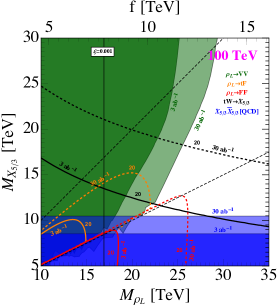
(b)  The results of LF${}_{\textbf{4}}$.

Figure 11: Left: the prospective reaches at the 27 TeV HE-LHC with integrated luminosities 3 ab^-1 and 15 ab^-1; Right: the prospective reaches at the 100 TeV $pp$ collider with integrated luminosities 3 ab^-1 and 30 ab^-1. The parameters and conventions are the same as Fig. 7.

Before we conclude our study, we make some estimates of the prospective reaches on the mass scales in our models at the 27 TeV HE-LHC and 100 TeV $pp$ collider. In Fig. 11, we have used the method described in Appendix E to extrapolate, based one the di-boson boosted-jet resonance searches at ATLAS ATL (2018a) and the pair top partner searches in the $1\ell+{\rm jets}$ channel at CMS Sirunyan et al. (2018a) in model LF${}_{\textbf{4}}$. We present the results with the integrated luminosities of 3 ab^-1 and 15 ab^-1 for the HE-LHC. For the 100 TeV collider, we show the results with 3 ab^-1 and 30 ab^-1 integrated luminosities. Compared with HL-LHC, we approximately gain a factor of 2 for the reach of the mass scales at the 15 ab^-1 HE-LHC and a factor of 5 at the 30 ab^-1 100 TeV collider. The SSDL channels (including $tW\rightarrow X_{5/3}$, $\rho\rightarrow tF$ and $\rho\rightarrow FF$) have slightly better reach at the 100 TeV collider with a factor of 5.5 gained with an integrated luminosity of 30 ab^-1.

IV Conclusion

In this paper, we have studied the phenomenology of the vector resonances and the fermionic resonances in several classes of benchmark simplified models in the minimal coset $SO(5)/SO(4)$, with some emphasis on the importance of the interplay of the phenomenology of the composite resonances. We have considered three irreducible representations under the unbroken $SO(4)$ for the spin-1 resonances: $\rho_{L}(\textbf{3},\textbf{1})$, $\rho_{R}(\textbf{1},\textbf{3})$, $\rho_{X}(\textbf{1},\textbf{1})$ and two irreducible representations for the spin-1/2 resonances: $\Psi_{\textbf{4}}(\textbf{2},\textbf{2})$, $\Psi_{\textbf{1}}(\textbf{1},\textbf{1})$. In addition, we have also studied the two scenarios depending on whether the right-handed top quark is elementary or fully composite.

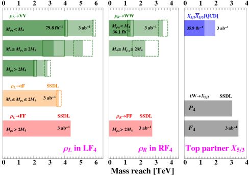
Figure 12: Summary of the present limits and prospective reach on the mass scales in models LF${}_{\textbf{4}}$ and RF${}_{\textbf{4}}$ for the benchmark parameters in Eq. (23) and Eq. (24). The bounds in models with partially composite $t_{R}$ are similar and not shown here except that for the single production of $X_{5/3}$, we have shown the bounds in both P${}_{\textbf{4}}$ and F${}_{\textbf{4}}$ scenarios. The bounds on $M_{\rho}$ are shown in three kinematical region ($M_{\rho}<M_{\textbf{4}}$, $M_{\textbf{4}}<M_{\rho}<2M_{\textbf{4}}$, $M_{\rho}>2M_{\textbf{4}}$). The rectangles for the existing searches $\rho_{L}\rightarrow VV$, $\rho_{R}\rightarrow WW$ indicate the ranges of the bound when varying the parameter $M_{\textbf{4}}$. The bounds from single production of $X_{5/3}$ are obtained by choosing $\xi=0.1$.

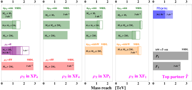
Figure 13: Summary of the present limits and prospective reach on the mass scales in models involving the singlet spin-1 resonance XP(F)${}_{\textbf{4},\textbf{1}}$ for the benchmark parameters in Eq. (25) and Eq. (26). The bounds on $M_{\rho}$ are shown in three kinematical region ($M_{\rho}<M_{\textbf{4}}$, $M_{\textbf{4}}<M_{\rho}<2M_{\textbf{4}}$, $M_{\rho}>2M_{\textbf{4}}$). The rectangles indicate the ranges of the bound when varying the parameter $M_{\textbf{4},\textbf{1}}$. The bounds from single production of $\tilde{T}$ are obtained by choosing $\xi=0.1$.

We have categorized the couplings of the composite resonances into four classes according to their expected sizes, $\mathcal{O}(g_{\rho})$, $\mathcal{O}(g_{\rho}s_{\theta_{L}}$, $g_{\rho}s_{\theta_{R}})$, $\mathcal{O}(g_{\rm SM})$, and $\mathcal{O}(g_{\rm SM}^{2}/g_{\rho})$, where $s_{\theta_{L,R}}$ are the elementary-composite mixing angles $s_{\theta_{L}},s_{\theta_{R}}$, and $g_{\rm SM}$ is of the size of the Standard Model gauge and Yukawa couplings. The results are summarized in Table 2, Table 3 and Table 4. Based on the discussion of the couplings, we have studied different production and decay channels for the composite resonances, paying special attention to the relevance of the cascade decay channels between the composite resonances. We have shown the present and future prospective bounds on our parameter space in the $M_{\rho}-M_{\Psi}$ plane in different models, focusing on the moderate large coupling $g_{\rho}=3$. We found that the cascade decay channels into one top partner and one top quark $t\Psi$ or two top partners $\Psi\Psi$ strongly affect the phenomenology of the $\rho$ if they are kinematically open. Their presence significantly weakens the reach of the channels with only SM particles, such as the di-boson channel. In addition, the decay channels $\rho^{+}_{L}\rightarrow t\bar{B}/X_{5/3}\bar{t}$ and $\rho^{+}_{L}\rightarrow X_{5/3}\bar{X}_{2/3}$, $\rho^{0}_{L,R,X}\rightarrow X_{5/3}\bar{X}_{5/3}$ can lead to the SSDL final states, which are used as an estimate of the reach on the $M_{\rho}-M_{\Psi}$ plane. We found that they are comparable in some regions of the parameter space to the di-boson searches or the top partner searches at the HL-LHC, especially for the $\rho_{L}$ models LP(F)${}_{\textbf{4}}$. For the $\rho_{R,X}$ models RP(F)${}_{\textbf{4}}$, XP(F)${}_{\textbf{4}}$, because the Drell-Yan production is suppressed by the smallness of the hypercharge gauge coupling, the cascade decay channels play less important roles. We also find that the SSDL channels in the single production of the charge-$5/3$ top partner $X_{5/3}$ can always play an important role in our parameter spaces. In the models involving the singlet spin-1 resonance XP(F)${}_{\textbf{4}}$ and XP(F)${}_{\textbf{1}}$, the associated production of top pair and the $\rho_{X}$ with the four top final states can play an important role, as the coupling between $\rho_{X}$ and $\bar{t}t$ is of $\mathcal{O}(g_{\rho})$ for the fully composite $t_{R}^{\rm(F)}$ models and $\mathcal{O}(g_{\rho}s^{2}_{\theta_{L}})$ or $\mathcal{O}(g_{\rho}s^{2}_{\theta_{R}})$ for the partially composite $t_{R}^{\rm(P)}$ models. We have recast the analysis in the SSDL channel by Ref. Liu and Mahbubani (2016) in our parameter space. In models XP(F)${}_{\textbf{1}}$, the single production of the top partner $\widetilde{T}$, followed by cascade decaying into $t\rho_{X}(t\bar{t})$ can be important in the region $M_{\widetilde{T}}>M_{\rho_{X}}$, and we have explored its sensitivity in the SSDL channel. It can be better than the $t\bar{t}\rho_{X}(t\bar{t})$ SSDL channel in model XP${}_{\textbf{1}}$. In the mass region $M_{\widetilde{T}}<M_{\rho_{X}}<2M_{\widetilde{T}}$, the $t\bar{t}$ fusion production of $\rho_{X}$, which decays into $t\overline{\widetilde{T}}$, can lead to the $t\bar{t}tbW^{+}$ final state with SSDL signature. We have used this to explore its sensitivity. In Fig. 12 and Fig. 13, we have summarized the prospective reach on the mass scale $M_{\rho}$ and $M_{\Psi}$ by the different existing searches at the LHC and by various SSDL channels from the cascade decays.

Several directions should be explored further. Among the various cascade decay channels, we have only considered the SSDL final state. The reach obtained this way is conservative. Other decay final states, such as $1\ell{\rm+jets}$, should also be studied in detail. The final kinematical variables are usually very complicated, and new techniques such as machine learning may be useful to enhance the sensitiy. We hope to address the issues in a future work.

V Acknowledgement

We would like to thank Andrea Tesi for the collaboration in the early stage of this work. KPX thanks Andrea Wulzer for useful discussions. KPX would like to thank the hospitality of the University of Chicago where part of this work was performed. LTW is supported by the DOE grant DE-SC0013642. DL is supported in part by the U.S. Department of Energy under Contract No. DE-AC02-06CH11357. KPX is supported in part by the National Science Foundation of China under Grant Nos. 11275009, 11675002, 11635001 and 11725520, and the National Research Foundation of Korea under grant 2017R1D1A1B03030820.

Appendix A CCWZ for SO(5)/SO(4) and its matching to BSM EFT

A.1 The CCWZ operators

We first present the $SO(5)$ generators as follows Panico and Wulzer (2016):

$$\begin{split}T^{\hat{i}}_{IJ}=&-\frac{i}{\sqrt{2}}\left(\delta^{\hat{i}I}\delta^{5J}-\delta^{\hat{i}J}\delta^{5I}\right),\\ T^{a_{L/R}}_{IJ}=&-\frac{i}{2}\left(\frac{1}{2}\epsilon^{abc}(\delta^{bI}\delta^{cJ}-\delta^{bJ}\delta^{cI})\pm(\delta^{aI}\delta^{4J}-\delta^{aJ}\delta^{4I})\right),\end{split}$$ (27)

where $\hat{i}=1,\cdots,4$, while $a,b,c=1,2,3$ and $I,J=1,\cdots,5$. Here $T^{a_{L}}$ and $T^{a_{R}}$ correspond to the unbroken $SO(4)\simeq SU(2)_{L}\times SU(2)_{R}$ generators and they are in the form of

$$T^{a_{L/R}}=\begin{pmatrix}t^{a_{L/R}}&0\\ 0&0\end{pmatrix},$$ (28)

with $t^{a_{L/R}}$ is the $4\times 4$ matrix, which will be useful in the following discussion.

The standard Callan-Coleman-Wess-Zumino (CCWZ) framwork Coleman et al. (1969); Callan et al. (1969) is used to describe the general interactions in our models. The Goldstone quartet $\vec{h}=(h_{1},h_{2},h_{3},h_{4})^{T}$ lives in the coset space $SO(5)/SO(4)$. The Goldstone matrix is defined as

$$U[\vec{h}]=e^{i\frac{\sqrt{2}}{f}h_{i}T^{\hat{i}}}=\begin{pmatrix}\delta_{ij}-(1-\cos\frac{h}{f})\frac{h_{i}h_{j}}{h^{2}}&\frac{h_{i}}{f}\sin\frac{h}{f}\\ -\frac{h_{j}}{f}\sin\frac{h}{f}&\cos\frac{h}{f}\end{pmatrix}.$$ (29)

Under the non-linearized $\mathcal{G}\in SO(5)$, it transforms as $U[\vec{h}]\to\mathcal{G}U[\vec{h}]\mathcal{H}^{-1}[\vec{h};\mathcal{G}]$, where $\mathcal{H}\in SO(4)$ is a function of the Goldstone fields and the global group element $\mathcal{G}$. We use the Maurer-Cartan form to define the covariant objects $d_{\mu}$ and $e_{\mu}$ as follows:

$$U^{\dagger}(A_{\mu}+i\partial_{\mu})U=d_{\mu}^{i}T^{\hat{i}}+e_{\mu}^{a}T^{a},$$ (30)

where $A_{\mu}\equiv A_{\mu}^{a}T^{a}$ are the gauge fields corresponding to the unbroken generators. The $d_{\mu}$ and $e_{\mu}$ objects will transform under the non-linearized $SO(5)$ group as:

$$d_{\mu}\to\mathcal{H}d_{\mu}\mathcal{H}^{-1},\quad e_{\mu}\to\mathcal{H}(e_{\mu}+i\partial_{\mu})\mathcal{H}^{-1}.$$ (31)

In MCHMs, only the subgroup $SU(2)_{L}\times U(1)_{Y}\in SO(4)\times U(1)_{X}$ is gauged, i.e.

$$A_{\mu}^{a_{L}}=g_{2}W_{\mu}^{a_{L}},\quad A_{\mu}^{1_{R},2_{R}}=0,\quad A_{\mu}^{3_{R}}=g_{1}B_{\mu},\quad X_{\mu}=g_{1}B_{\mu}.$$ (32)

The last gauge field $X_{\mu}$, corresponding to the $U(1)_{X}$ group, is introduced to give correct hypercharge for the fermions, and the Goldstone bosons are neutral under this symmetry.

The full formulae of $d_{\mu}$ and $e_{\mu}$ symbols can be obtained as follows Panico and Wulzer (2016)

$$\begin{split}d_{\mu}^{i}=&\sqrt{2}\left(\frac{1}{|\vec{h}|}\sin\frac{|\vec{h}|}{f}-\frac{1}{f}\right)\frac{\vec{h}^{T}D_{\mu}\vec{h}}{|\vec{h}|^{2}}\vec{h}_{i}-\frac{\sqrt{2}}{|\vec{h}|}\sin\frac{|\vec{h}|}{f}D_{\mu}\vec{h}_{i},\\ e_{\mu}^{a_{L}}=&g_{2}W^{a_{L}}_{\mu}-\frac{4}{|\vec{h}|^{2}}\sin^{2}\frac{|\vec{h}|}{2f}\vec{h}^{T}it^{a_{L}}D_{\mu}\vec{h},\\ e_{\mu}^{a_{R}}=&\delta^{a3}g_{1}B_{\mu}-\frac{4}{|\vec{h}|^{2}}\sin^{2}\frac{|\vec{h}|}{2f}\vec{h}^{T}it^{a_{R}}D_{\mu}\vec{h},\end{split}$$ (33)

where the covariant derivative is given by:

$$D_{\mu}\vec{h}=(\partial_{\mu}-ig_{2}t^{a_{L}}W_{\mu}^{a_{L}}-ig_{1}t^{3_{R}}B_{\mu})\vec{h},$$ (34)

and the matrices $t^{a_{L/R}}$ are defined in Eq. (28). Because of Eq. (31), the leading Lagrangian of the Goldstone fields is simply

$$\mathcal{L}^{d_{2}}=\frac{f^{2}}{4}d_{\mu}^{i}d^{i\mu}.$$ (35)

For the fermionic heavy resonances, they fall into the irreducible representations of the unbroken group $SO(4)\times U(1)_{X}\simeq SU(2)_{L}\times SU(2)_{R}\times U(1)_{X}$. We will consider two irreducible representations: the quartet $\textbf{4}_{2/3}$ and the singlet $\textbf{1}_{2/3}$ as the lightest top partners. They are parametrized as follows:

$$\Psi_{\textbf{4}}=\frac{1}{\sqrt{2}}\left(\begin{array}[]{c}iB-iX_{5/3}\\ B+X_{5/3}\\ iT+iX_{2/3}\\ -T+X_{2/3}\end{array}\right)_{2/3},\quad\Psi_{\textbf{1}}=\begin{pmatrix}\widetilde{T}\end{pmatrix}_{2/3},$$ (36)

and transform as $\Psi\to\mathcal{H}_{\textbf{r}_{\Psi}}\otimes\mathcal{G}_{X}\Psi$, where $\textbf{r}_{\Psi}$ is the $SO(4)$ representation of $\Psi$, and $\mathcal{G}_{X}$ denotes the group element of $U(1)_{X}$. From the transformation rules in Eq. (31), we can construct a covariant derivative acting on the composite fermionic fields $\Psi$:

$$\nabla_{\mu}=\partial_{\mu}-ie_{\mu}^{a}T^{a}_{\textbf{r}_{\Psi}}.$$ (37)

Taking into account of the $U(1)_{X}$ group, the covariant derivative becomes $(\nabla_{\mu}-ig_{1}XB_{\mu})$. For the spin-1 resonances, we consider three irreducible representations under the unbroken $SO(4)$: $\rho_{L}(\textbf{3},\textbf{1})$, $\rho_{R}(\textbf{1},\textbf{3})$ and $\rho_{X}(\textbf{1},\textbf{1})$.

A.2 The matching to the Higgs doublet notation

The CCWZ operators and the effective Lagrangians for the composite resonances can be written in terms of the fields that have the definite quantum number under the SM gauge group $SU(2)_{L}\times U(1)_{Y}$ . To see this, we first notice that the SM Higgs doublet with hypercharge $Y=1/2$ can be written as follows:

$$H=\begin{pmatrix}\frac{h_{2}+ih_{1}}{\sqrt{2}}\\ \frac{h_{4}-ih_{3}}{\sqrt{2}}\end{pmatrix},\quad\widetilde{H}=i\sigma^{2}H^{*}.$$ (38)

It is related with the quartet notation $\vec{h}$ by an unitary matrix $P$ with determinant -1:

$$\vec{h}=P\begin{pmatrix}H\\ -\widetilde{H}\end{pmatrix},\quad P=\begin{pmatrix}-\frac{i}{\sqrt{2}}&0&0&\frac{i}{\sqrt{2}}\\ \frac{1}{\sqrt{2}}&0&0&\frac{1}{\sqrt{2}}\\ 0&\frac{i}{\sqrt{2}}&\frac{i}{\sqrt{2}}&0\\ 0&\frac{1}{\sqrt{2}}&-\frac{1}{\sqrt{2}}&0\end{pmatrix},\quad P^{\dagger}P=\mathbb{I}_{4},\quad\text{Det}\,P=-1.$$ (39)

The $SO(4)$ generators can be converted to the doublet notation by using $P$:

$$\begin{split}P^{\dagger}t^{a_{L}}P&=\begin{pmatrix}\frac{1}{2}\sigma^{a_{L}}&\\ &\frac{1}{2}\sigma^{a_{L}}\end{pmatrix},\quad P^{\dagger}t^{3_{R}}P=\begin{pmatrix}\frac{1}{2}\mathbb{I}_{2\times 2}&\\ &-\frac{1}{2}\mathbb{I}_{2\times 2}\end{pmatrix},\\ P^{\dagger}t^{1_{R}}P&=\begin{pmatrix}&\frac{1}{2}\mathbb{I}_{2\times 2}\\ \frac{1}{2}\mathbb{I}_{2\times 2}&\end{pmatrix},\quad P^{\dagger}t^{2_{R}}P=\begin{pmatrix}&-\frac{i}{2}\mathbb{I}_{2\times 2}\\ \frac{i}{2}\mathbb{I}_{2\times 2}&\end{pmatrix}.\end{split}$$ (40)

Consequently, the $\vec{h}$ covariant derivative term can be rewritten as:

$$D_{\mu}\vec{h}=P\begin{pmatrix}D_{\mu}H\\ -D_{\mu}\widetilde{H}\end{pmatrix},$$ (41)

where the $D_{\mu}$ in the right-hand side of the equation is the normal SM covariant derivative:

$$D_{\mu}=\partial_{\mu}-ig_{2}\frac{\sigma^{a_{L}}}{2}W_{\mu}^{a_{L}}-ig_{1}YB_{\mu}.$$ (42)

where hypercharge $Y$ is given by $Y=T^{3_{R}}+X$. Using above results, we can easily rewrite the leading Lagrangian in Eq. (35) in the doublet notation:

$$\frac{f^{2}}{4}d_{\mu}^{i}d^{i\mu}=\frac{f^{2}}{2|H|^{2}}\sin^{2}\frac{\sqrt{2}|H|}{f}D_{\mu}H^{\dagger}D^{\mu}H+\frac{f^{2}}{8|H|^{4}}\left(\frac{2|H|^{2}}{f^{2}}-\sin^{2}\frac{\sqrt{2}|H|}{f}\right)(\partial_{\mu}|H|^{2})^{2},$$ (43)

with $|H|=\sqrt{H^{\dagger}H}$. For further convenience, we list the following useful identities:

$$\begin{split}&\vec{h}^{T}D_{\mu}\vec{h}=\partial_{\mu}(H^{\dagger}H),\quad\vec{h}^{T}t^{a_{L}}D_{\mu}\vec{h}=\frac{1}{2}H^{\dagger}\sigma^{a_{L}}\mathord{\buildrel\lower 3.0pt\hbox{$\scriptscriptstyle\leftrightarrow$}\over{D}_{\mu}}H,\quad\vec{h}^{T}t^{3_{R}}D_{\mu}\vec{h}=\frac{1}{2}H^{\dagger}\mathord{\buildrel\lower 3.0pt\hbox{$\scriptscriptstyle\leftrightarrow$}\over{D}_{\mu}}H,\\ &\vec{h}^{T}t^{1_{R}}D_{\mu}\vec{h}=-\frac{1}{2}(\widetilde{H}^{\dagger}D_{\mu}H-D_{\mu}H^{\dagger}\widetilde{H}),\quad\vec{h}^{T}t^{2_{R}}D_{\mu}\vec{h}=\frac{i}{2}(H^{\dagger}D_{\mu}\widetilde{H}+D_{\mu}\widetilde{H}^{\dagger}H).\end{split}$$ (44)

where the $\mathord{\buildrel\lower 3.0pt\hbox{$\scriptscriptstyle\leftrightarrow$}\over{D}_{\mu}}$ is defined as:

$$H^{\dagger}\mathord{\buildrel\lower 3.0pt\hbox{$\scriptscriptstyle\leftrightarrow$}\over{D}_{\mu}}H\equiv H^{\dagger}(D_{\mu}H)-(D_{\mu}H^{\dagger})H;\quad H^{\dagger}\sigma^{a_{L}}\mathord{\buildrel\lower 3.0pt\hbox{$\scriptscriptstyle\leftrightarrow$}\over{D}_{\mu}}H\equiv H^{\dagger}\sigma^{a_{L}}(D_{\mu}H)-(D_{\mu}H^{\dagger})\sigma^{a_{L}}H.$$ (45)

The quartet top partner fields, $\Psi_{\textbf{4}}$ can be decomposed as two $SU(2)_{L}$ doublets with hypercharge $Y=1/6$, $7/6$ as follows:

$$\Psi_{\textbf{4}}=P\begin{pmatrix}Q_{X}\\ Q\end{pmatrix},\qquad Q=\begin{pmatrix}T\\ B\end{pmatrix}_{1/6},\quad Q_{X}=\begin{pmatrix}X_{5/3}\\ X_{2/3}\end{pmatrix}_{7/6},$$ (46)

with the same $P$ matrix as defined in Eq. (39). The SM fermions are assumed to be embedded in the $\textbf{5}_{X}$ representation of $SO(5)\times U(1)_{X}$ with hypercharge given by $Y=T^{3_{R}}+X$. We only consider the top sector in our paper. For the SM $SU(2)$ doublet $q_{L}=(t_{L},b_{L})^{T}$, we have the embedding:

$$q_{L}^{\textbf{5}}=\frac{1}{\sqrt{2}}\begin{pmatrix}ib_{L}&b_{L}&it_{L}&-t_{L}&0\end{pmatrix}^{T}_{2/3}=P_{\textbf{5}}\begin{pmatrix}0,0,t_{L},b_{L},0\end{pmatrix}^{T},\quad P_{\textbf{5}}=\begin{pmatrix}P&0_{4\times 1}\\ 0_{1\times 4}&1\end{pmatrix}.$$ (47)

The $q_{L}^{\textbf{5}}$ formally transforms under the $\mathcal{G}\in SO(5)$ and $\mathcal{G}_{X}\in U(1)_{X}$ as $q_{L}^{\textbf{5}}\rightarrow\mathcal{G}\otimes\mathcal{G}_{X}q_{L}^{\textbf{5}}$. For the right-handed top quark, we will consider two possibilities: $t_{R}$ as an elementary filed or as a massless bound state of the strong sector. In the first case, we also embed it in the representation of $\textbf{5}_{2/3}$:

$$t_{R}^{\textbf{5}}=\begin{pmatrix}0&0&0&0&t_{R}^{\rm(P)}\end{pmatrix}^{T}_{2/3}.$$ (48)

For the fully composite right-handed top quark, we assume that it is a singlet of $SO(4)$, denoted as $t_{R}^{\rm(F)}$ and its interactions preserve the non-linearized $SO(5)$. We denote those two treatments as partially and fully composite $t_{R}$ scenario, respectively.

All the effective Lagrangian in MCHMs can be rewritten in terms of the doublet notation easily using Eq. (33), Eq. (44), Eq. (46), Eq. (47) and Eq. (48). The full results are tedious, thus we will not list them here; however, their LO expansions in $H^{\dagger}H/f^{2}$ order will be listed and discussed in Appendix B.

Appendix B The models

In this section, we briefly describe the models considered in our paper (see Refs. Greco and Liu (2014); De Simone et al. (2013); Contino et al. (2011)). We focus on the minimal coset $SO(5)\times U(1)_{X}/SO(4)\times U(1)_{X}$ of the strong sector, where the Higgs bosons are the pseudo-Nambu-Goldstone bosons associated with this global symmetry breaking.

B.1 The models involving $\rho_{L}(3,1)$ and quartet top partners $\Psi_{\textbf{4}}(2,2)$: LP(F)₄

We start from the models involving the $\rho_{L}$ and the quartet top partners $\Psi_{\textbf{4}}$. The Lagrangian of the strong sector reads:

$$\begin{split}\mathcal{L}^{\text{L}_{\textbf{4}}}=&-\frac{1}{4}\rho_{\mu\nu}^{a_{L}}\rho^{a_{L}\mu\nu}+\frac{m_{\rho_{L}}^{2}}{2g_{\rho_{L}}^{2}}(g_{\rho_{L}}\rho_{\mu}^{a_{L}}-e_{\mu}^{a_{L}})^{2}+\bar{\Psi}_{\textbf{4}}\gamma^{\mu}i\left(\nabla_{\mu}-ig_{1}\frac{2}{3}B_{\mu}\right)\Psi_{\textbf{4}}-M_{\textbf{4}}\bar{\Psi}_{\textbf{4}}\Psi_{\textbf{4}}\\ &+c_{1}\bar{\Psi}_{\textbf{4}}\gamma^{\mu}t^{a_{L}}\Psi_{\textbf{4}}(g_{\rho_{L}}\rho^{a_{L}}_{\mu}-e^{a_{L}}_{\mu}),\end{split}$$ (49)

where the field strength of the spin-1 resonance is defined as

$$\rho_{\mu\nu}^{a_{L}}=\partial_{\mu}\rho^{a_{L}}_{\nu}-\partial_{\nu}\rho^{a_{L}}_{\mu}+g_{\rho_{L}}\epsilon^{a_{L}b_{L}c_{L}}\rho_{\mu}^{b_{L}}\rho_{\nu}^{c_{L}}.$$ (50)

The Yukawa interactions between strong and elementary sector are:

$$\begin{split}\mathcal{L}^{\text{P}_{\textbf{4}}}=&y_{L}f\bar{q}_{L}^{\textbf{5}I}U_{Ij}\Psi_{\textbf{4}}^{j}+y_{R}f\bar{t}_{R}^{\textbf{5}I}U_{Ij}\Psi_{\textbf{4}}^{j}+\text{h.c.},\\ \mathcal{L}^{\text{F}_{\textbf{4}}}=&(c_{2}\bar{\Psi}_{\textbf{4}}^{i}\gamma^{\mu}id^{i}_{\mu}t_{R}^{\rm(F)}+\text{h.c.})+(y_{L}f\bar{q}_{L}^{\textbf{5}I}U_{Ij}\Psi_{\textbf{4}}^{j}+y_{2L}f\bar{q}_{L}^{\textbf{5}I}U_{I5}t_{R}^{\rm(F)}+\text{h.c.}).\end{split}$$ (51)

The fully Lagrangian is then written as Greco and Liu (2014); De Simone et al. (2013); Contino et al. (2011)

$$\mathcal{L}^{\text{LP}_{\textbf{4}}}=\mathcal{L}^{\text{L}_{\textbf{4}}}+\mathcal{L}^{\text{P}_{\textbf{4}}};\quad\mathcal{L}^{\text{LF}_{\textbf{4}}}=\mathcal{L}^{\text{L}_{\textbf{4}}}+\mathcal{L}^{\text{F}_{\textbf{4}}},$$ (52)

where we omitted the SM Lagrangians for the quark fields $q_{L}$ and $t_{R}$. Note that the CCWZ covariant objects $e_{\mu}^{a}$ include the SM gauge fields:

$$\begin{split}e_{\mu}^{a_{L}}&=g_{2}W_{\mu}^{a_{L}}-\frac{i}{f^{2}}H^{\dagger}\frac{\sigma^{a_{L}}}{2}\mathord{\buildrel\lower 3.0pt\hbox{$\scriptscriptstyle\leftrightarrow$}\over{D}_{\mu}}H+\cdots,\\ e_{\mu}^{3_{R}}&=g_{1}B_{\mu}-\frac{i}{2f^{2}}H^{\dagger}\mathord{\buildrel\lower 3.0pt\hbox{$\scriptscriptstyle\leftrightarrow$}\over{D}_{\mu}}H+\cdots\end{split}$$ (53)

and we have written the formulae in terms of SM Higgs doublet $H$ (see Appendix A for the definition and derivation). Note that the SM gauge interactions don’t preserve the non-linearly realized $SO(5)$ symmetry and provide the explicit breaking, thus will contribute to the Higgs potential at one-loop level. The term with coefficient $c_{1}$ involves the direct coupling between the $\rho_{L}$ and the quartet top partners at the order of $g_{\rho_{L}}$. As discussed in Ref. Greco and Liu (2014), this interaction will have an important impact on the phenomenology of $\rho_{L}$ especially when $m_{\rho_{L}}>2M_{\textbf{4}}$ and decaying into two top partners are allowed. In most of the case, we will choose $c_{1}=1$ as our benchmark point.

Note that the mass term for the $\rho_{L}$ in Eq. (49) will induce a linear mixing between them and the SM $W_{\mu}$ gauge bosons before EWSB. Diagonalizing the mass matrix will lead to the partial compositeness of $\mathcal{O}(g_{2}/g_{\rho_{L}})$ for the $W$ bosons. As a result, the SM $SU(2)_{L}$ gauge coupling will be redefined as follows:

$$\frac{1}{g^{2}}=\frac{1}{g_{2}^{2}}+\frac{1}{g_{\rho_{L}}^{2}},$$ (54)

and the $W$-mass at the LO is given by (see Appendix C for detail):

$$M_{W}^{2}=\frac{1}{4}g^{2}v^{2},\quad v=f\sin\frac{\left<h\right>}{f}=246~{}\text{GeV}.$$ (55)

Due to the linear mixing, the mass of the $\rho_{L}$ will also be modified as follows:

$$M_{\rho_{L}}^{2}=m_{\rho_{L}}^{2}\left(1+\frac{g_{2}^{2}}{g_{\rho_{L}}^{2}}\right).$$ (56)

Note that this direct mixing mass term will also lead to contribution to $\hat{S}$-parameter in the low energy observable. Actually, integrating out the $\rho_{L}$ at the LO, we will obtain the $\mathcal{O}_{W}$ operator (see Ref. Greco and Liu (2014)), which leads to the contribution to the $\hat{S}$ parameter Barbieri et al. (2004):

$$\hat{S}=\frac{M_{W}^{2}}{g_{\rho_{L}}^{2}f^{2}}.$$ (57)

The $\rho_{L}$ resonance will be coupled to SM fermions universally with strength of $\mathcal{O}(g^{2}/g_{\rho_{L}})$ due to the linear mixing. The non-universality comes from the linear mixing between the SM fermions and corresponding composite partners. Since the mixing is the source of the SM fermion masses after EWSB, it is roughly the order of the fermion Yukawa couplings. Thus we expect that only the third generation mixings (especially the top quark) have the important impact on phenomenology of the $\rho_{L}$, which is the reason we only focus on the top sector.

For the partially composite right-handed top quark scenario, we have two parameters $y_{L}$, $y_{R}$ controlling the mixing between $q_{L}$, $t_{R}^{\rm(P)}$ and the top partner $\Psi_{\textbf{4}}$. Similar to the SM gauge bosons, there will be direct mixing between $q_{L}$ and the composite $SU(2)_{L}$ doublet $Q$ before EWSB proportional to $y_{L}$:

$$y_{L}f\bar{q}_{L}Q_{R}+{\rm h.c.},$$ (58)

where the doublet $Q=(T,B)^{T}$ is defined in Eq. (46). This motives us to define a left-handed mixing angle $\theta_{L}$ as follows:

$$\tan\theta_{L}=\frac{y_{L}f}{M_{\textbf{4}}},$$ (59)

which measures the partial compositeness of the SM fermions $q_{L}$. Due to the linear mixing, the mass formulae for the fermionic resonances before EWSB are given by:

$$M_{Q}=\sqrt{M_{\textbf{4}}^{2}+y_{L}^{2}f^{2}},\quad M_{Q_{X}}=M_{\textbf{4}}.$$ (60)

Note that $y_{L}$ breaks the $SO(4)$ explicitly and will contribute to the $\hat{T}$ parameter at the loop level, thus can’t be too large. In contrast, $t_{R}^{\rm(P)}$ is an $SO(4)$ singlet so that $y_{R}$ term preserves the custodial symmetry can in principle can be large Ghosh et al. (2017). For the fully composite $t_{R}^{\rm(F)}$, besides the mixing between $q_{L}$ and $\Psi_{\textbf{4}}$ (denoted also as $y_{L}$), we can write a direct coupling $y_{2L}$ between $q_{L}$ and $t_{R}^{\rm(F)}$. This term provides the main source of top quark mass. Since $t_{R}^{\rm(F)}$ belongs to the strong sector, there are also direct interactions between it and the composite resonances, which are written as the $c_{2}$ term in the $\mathcal{L}^{\text{F}_{\textbf{4}}}$. As discussed in LABEL:DeSimone:2012fs, this strong interaction term provides the dominant contribution to decay of the top partners, especially when the mixing parameters are small.

Note that it will be very useful to rewrite the Lagrangian in terms of SM $SU(2)_{L}\times U(1)_{Y}$ notation, where the SM gauge symmetries are manifest. By using the formulae of the Goldstone matrix $U$ and the $d_{\mu},e_{\mu}$ in the Appendix A, we can write the Lagrangian $\mathcal{L}^{\text{L}_{\textbf{4}}}$ using the doublet notation as follows:

$$\begin{split}\mathcal{L}^{\text{L}_{\textbf{4}}}=&-\frac{1}{4}\rho_{\mu\nu}^{a_{L}}\rho^{a_{L}\mu\nu}+\frac{a_{\rho_{L}}^{2}}{2}f^{2}\left(g_{\rho_{L}}\rho_{\mu}^{a_{L}}-g_{2}W_{\mu}^{a_{L}}+\frac{i}{f^{2}}H^{\dagger}\frac{\sigma^{a_{L}}}{2}\mathord{\buildrel\lower 3.0pt\hbox{$\scriptscriptstyle\leftrightarrow$}\over{D}_{\mu}}H\right)^{2}\\ &+\bar{Q}(\gamma^{\mu}iD_{\mu}-M_{\textbf{4}})Q+\bar{Q}_{X}(\gamma^{\mu}iD_{\mu}-M_{\textbf{4}})Q_{X}\\ &-\frac{i}{4f^{2}}\left(\bar{Q}_{X}\gamma^{\mu}\sigma^{a_{L}}Q_{X}+\bar{Q}\gamma^{\mu}\sigma^{a_{L}}Q\right)H^{\dagger}\sigma^{a_{L}}\mathord{\buildrel\lower 3.0pt\hbox{$\scriptscriptstyle\leftrightarrow$}\over{D}_{\mu}}H\\ &-\frac{i}{4f^{2}}\left(\bar{Q}_{X}\gamma^{\mu}Q_{X}-\bar{Q}\gamma^{\mu}Q\right)H^{\dagger}\mathord{\buildrel\lower 3.0pt\hbox{$\scriptscriptstyle\leftrightarrow$}\over{D}_{\mu}}H+\left(\frac{i}{4f^{2}}\bar{Q}\gamma^{\mu}Q_{X}H^{\dagger}\mathord{\buildrel\lower 3.0pt\hbox{$\scriptscriptstyle\leftrightarrow$}\over{D}_{\mu}}\widetilde{H}+\text{h.c.}\right)\\ &+c_{1}\left(\bar{Q}\gamma^{\mu}\frac{\sigma^{a_{L}}}{2}Q+\bar{Q}_{X}\gamma^{\mu}\frac{\sigma^{a_{L}}}{2}Q_{X}\right)\left(g_{\rho_{L}}\rho_{\mu}^{a_{L}}-g_{2}W_{\mu}^{a_{L}}+\frac{i}{f^{2}}H^{\dagger}\frac{\sigma^{a_{L}}}{2}\mathord{\buildrel\lower 3.0pt\hbox{$\scriptscriptstyle\leftrightarrow$}\over{D}_{\mu}}H\right)+\cdots,\end{split}$$ (61)

where the $\cdots$ denotes the higher order terms in $H^{\dagger}H/f^{2}$ and we have defined the $\mathcal{O}(1)$ parameter $a_{\rho_{L}}$ as in LABEL:Contino:2011np:

$$a_{\rho_{L}}=\frac{m_{\rho_{L}}}{g_{\rho_{L}}f}.$$ (62)

From the dimension-six operators involving the top partners and the Higgs fields, we can see that generally the gauge couplings of the top partners are modified at the $\mathcal{O}(\xi)$ after EWSB. Note that there is an accidental parity symmetry $P_{LR}$ in the kinetic Lagrangian for the quartet top partner defined as Agashe et al. (2006):

$$P_{LR}^{(4)}=\text{diag}(-1,-1,-1,1),$$ (63)

and the couplings between eigenstates of this parity ($X_{5/3},B$) and the SM $Z$ gauge bosons will not obtain any modification after EWSB. This can be easily seen by using the formulae for the currents in the vacuum:

$$\begin{split}iH^{\dagger}\mathord{\buildrel\lower 3.0pt\hbox{$\scriptscriptstyle\leftrightarrow$}\over{D}_{\mu}}H&\to-\frac{\left<h\right>^{2}}{2}\left(g_{2}W_{\mu}^{3}-g_{1}B_{\mu}\right),\\ iH^{\dagger}\sigma^{a_{L}}\mathord{\buildrel\lower 3.0pt\hbox{$\scriptscriptstyle\leftrightarrow$}\over{D}_{\mu}}H&\to\frac{\left<h\right>^{2}}{2}\left(g_{2}W_{\mu}^{a_{L}}-g_{1}\delta^{a3}B_{\mu}\right),\\ \end{split}$$ (64)

remembering that $T^{3_{L}}(X_{5/3})=T^{3_{R}}(X_{5/3})=1/2$ and $T^{3_{L}}(B)=T^{3_{R}}(B)=-1/2$. This is important because $ZB_{L}\bar{B}_{L}$ are not modified by the Higgs VEV means that after the mixing between $b_{L}$ and $B_{L}$, the $Zb_{L}\bar{b}_{L}$ remains the same as the SM canonical couplings .

Similarly, we can write the elementary-composite mixing Lagrangian $\mathcal{L}^{P_{4}}$ in the doublet notation:

$$\mathcal{L}^{\text{P}_{\textbf{4}}}=y_{L}f\left(\bar{q}_{L}Q_{R}+\frac{1}{2f^{2}}\bar{q}_{L}\widetilde{H}\,(H^{\dagger}Q_{XR}-\tilde{H}^{\dagger}Q_{R})\right)+y_{R}\left(\bar{Q}_{L}\widetilde{H}t_{R}^{\rm(P)}-\bar{Q}_{L}^{X}Ht_{R}^{\rm(P)}\right)+\text{h.c.}$$ (65)

where we only keep the leading terms in the expansion of $H^{\dagger}H/f^{2}$. We can see clearly that after EWSB only the mass matrix in the top sector obtains corrections of $\mathcal{O}(y_{L}f\xi,y_{R}v)$, while for the charge $-1/3$ and charge-$5/3$ resonances, their mass formulae are not modified . After EWSB, the top mass is given by:

$$M_{t}=\frac{y_{R}vs_{\theta_{L}}}{\sqrt{2}}+\cdots,$$ (66)

where $s_{\theta_{L}}$ denotes $\sin\theta_{L}$ defined in Eq. (59). The EWPT at the LEP prefers $y_{L}\lesssim y_{R}$, thus $y_{R}$ mixing term is dominant. In the unitary gauge, this term becomes:

$$\frac{y_{R}}{\sqrt{2}}(\left<h\right>+h)\left(\bar{T}_{L}-\bar{X}_{2/3L}\right)t_{R}^{\rm(P)}.$$ (67)

So in the large $y_{R}$ limit, there will be a top partner (the heavier one) in the mass eigenstate, which will primarily decay into $th$ and the other one will primarily decay into $tZ$. See Appendix C for detail, where we summarize the mass matrices and mass formulae. As we will discuss below, in our consideration, we will focus on the region $y_{R}\gtrsim 1$, this effect will not be manifest. For the fully composite $t_{R}^{\rm(F)}$ case, we have:

$$\begin{split}\mathcal{L}^{\text{F}_{\textbf{4}}}=&-c_{2}\frac{\sqrt{2}}{f}(\bar{Q}_{XR}\gamma^{\mu}t_{R}iD_{\mu}H-\bar{Q}_{R}\gamma^{\mu}t_{R}iD_{\mu}\widetilde{H}+\text{h.c.}).\\ &+y_{L}f\left(\bar{q}_{L}Q_{R}+\frac{1}{2f^{2}}\bar{q}_{L}\widetilde{H}\,(H^{\dagger}Q_{XR}-\tilde{H}^{\dagger}Q_{R})\right)-y_{2L}\bar{q}_{L}\widetilde{H}t_{R}^{\rm(F)}+\text{h.c.},\\ \end{split}$$ (68)

The top mass to the leading order is given by:

$$M_{t}=\frac{y_{2L}c_{\theta_{L}}v}{\sqrt{2}}+\cdots,$$ (69)

where $c_{\theta_{L}}$ denotes $\cos\theta_{L}$ defined in Eq. (59). So that the top Yukawa coupling is mainly determined by $y_{2L}$, which is different with partially composite $t_{R}^{\rm(P)}$ case.

B.2 The models involving $\rho_{R}(1,3)$ and quartet top partners $\Psi_{\textbf{4}}(2,2)$: RP(F)${}_{\textbf{4}}$

For the $\rho_{R}$ models, the effective Lagrangians read:

$$\begin{split}\mathcal{L}^{\text{R}_{\textbf{4}}}=&-\frac{1}{4}\rho_{\mu\nu}^{a_{R}}\rho^{a_{R}\mu\nu}+\frac{m_{\rho_{R}}^{2}}{2g_{\rho_{R}}^{2}}(g_{\rho_{R}}\rho_{\mu}^{a_{R}}-e_{\mu}^{a_{R}})^{2}+\bar{\Psi}_{\textbf{4}}\gamma^{\mu}i\left(\nabla_{\mu}-ig_{1}\frac{2}{3}B_{\mu}\right)\Psi_{\textbf{4}}-M_{\textbf{4}}\bar{\Psi}_{\textbf{4}}\Psi_{\textbf{4}}\\ &+c_{1}\bar{\Psi}_{\textbf{4}}\gamma^{\mu}t^{a_{R}}\Psi_{\textbf{4}}(g_{\rho_{R}}\rho^{a_{R}}_{\mu}-e^{a_{R}}_{\mu});\end{split}$$ (70)

where the definition of $\rho_{\mu\nu}^{a_{R}}$ is the same as in Eq. (50) with $(L\to R)$. The effective Lagrangians in models RP(F)${}_{\textbf{4}}$ are given by:

$$\mathcal{L}^{\text{RP}_{\textbf{4}}}=\mathcal{L}^{\text{R}_{\textbf{4}}}+\mathcal{L}^{\text{P}_{\textbf{4}}};\quad\mathcal{L}^{\text{RF}_{\textbf{4}}}=\mathcal{L}^{\text{R}_{\textbf{4}}}+\mathcal{L}^{\text{F}_{\textbf{4}}},$$ (71)

where the Lagrangians $\mathcal{L}^{{\rm P(F)}_{\textbf{4}}}$ are the same as in Eq. (49). In terms of doublet notation, we have:

$$\begin{split}\mathcal{L}^{\rm R_{\textbf{4}}}=&-\frac{1}{4}\rho_{\mu\nu}^{a_{R}}\rho^{a_{R}\mu\nu}+\frac{a_{\rho_{R}}^{2}}{2}f^{2}\left(g_{\rho_{R}}\rho_{\mu}^{3_{R}}-g_{1}B_{\mu}+\frac{1}{2f^{2}}H^{\dagger}i\mathord{\buildrel\lower 3.0pt\hbox{$\scriptscriptstyle\leftrightarrow$}\over{D}_{\mu}}H\right)^{2}\\ &+\frac{a_{\rho_{R}}^{2}}{2}f^{2}\left(\sqrt{2}g_{\rho_{R}}\rho_{\mu}^{-_{R}}-\frac{1}{2f^{2}}H^{\dagger}i\mathord{\buildrel\lower 3.0pt\hbox{$\scriptscriptstyle\leftrightarrow$}\over{D}_{\mu}}\widetilde{H}\right)\left(\sqrt{2}g_{\rho_{R}}\rho_{\mu}^{+_{R}}-\frac{1}{2f^{2}}\widetilde{H}^{\dagger}i\mathord{\buildrel\lower 3.0pt\hbox{$\scriptscriptstyle\leftrightarrow$}\over{D}_{\mu}}H\right)\\ &+c_{1}\left(\frac{1}{2}\bar{Q}_{X}\gamma^{\mu}Q_{X}-\frac{1}{2}\bar{Q}\gamma^{\mu}Q\right)\left(g_{\rho_{R}}\rho_{\mu}^{3_{R}}-g_{1}B_{\mu}+\frac{1}{2f^{2}}H^{\dagger}i\mathord{\buildrel\lower 3.0pt\hbox{$\scriptscriptstyle\leftrightarrow$}\over{D}_{\mu}}H\right)\\ &+c_{1}\frac{1}{2}\bar{Q}\gamma^{\mu}Q_{X}\left(\sqrt{2}g_{\rho_{R}}\rho_{\mu}^{-_{R}}-\frac{1}{2f^{2}}H^{\dagger}i\mathord{\buildrel\lower 3.0pt\hbox{$\scriptscriptstyle\leftrightarrow$}\over{D}_{\mu}}\widetilde{H}\right)+\text{h.c.}+\cdots,\end{split}$$ (72)

where we only show the terms involving the $\rho_{R}$ and defined:

$$a_{\rho_{R}}=\frac{m_{\rho_{R}}}{g_{\rho_{R}}f}.$$ (73)

Note that similar with $\rho_{L}$, there is a direct mixing between $\rho^{3R}_{\mu}$ and the hypercharge field $B_{\mu}$. So the $U(1)_{Y}$ gauge coupling is redefined as follows:

$$\frac{1}{g^{\prime 2}}=\frac{1}{g_{1}^{2}}+\frac{1}{g_{\rho_{R}}^{2}},$$ (74)

and the $Z$-mass to the LO is given by:

$$M_{Z}^{2}=\frac{g^{2}+g^{\prime 2}}{4}v^{2},\quad g=g_{2},$$ (75)

Note that this direct mixing mass term will also lead to contribution to $\hat{S}$-parameter in the low energy observable: integrating out the $\rho_{R}$ will result in the $\mathcal{O}_{B}$ operator and

$$\hat{S}=\frac{M_{W}^{2}}{g_{\rho_{R}}^{2}f^{2}}.$$ (76)

As can been seen from Eq. (72), for the neutral resonance $\rho^{3_{R}}$, it has the universal coupling of $\mathcal{O}(g^{\prime 2}/g_{\rho_{R}})$ to the SM fermions, while for the charged $\rho_{R}$, its coupling arise from $\mathcal{O}(\xi)$. This makes $\rho_{R}^{0}$ more produced at the LHC than the charged one and thus the most stringent constraint on the $\rho_{R}$ models comes from the neutral spin-1 resonance searches. Because of the smallness of $U(1)_{Y}$ gauge coupling $g^{\prime}$ compared with $SU(2)_{L}$ gauge coupling $g$, its constraints are weaker than $\rho_{L}$. For the direct interactions with the fermionic resonances (the $c_{1}$ term), they are similar to the $\rho_{L}$ interactions except that the charged currents are between $Q$ and $Q_{X}$.

B.3 The models involving $\rho_{X}(1,1):$ XP(F)${}_{\textbf{4}}$ and XP(F)${}_{\textbf{1}}$

For the models involving the $\rho_{X}$ and the quartet $\Psi_{\textbf{4}}$, the Lagrangian containing the $\rho_{X}$ are given by:

$$\begin{split}\mathcal{L}^{\rm X_{\textbf{4}}}=&-\frac{1}{4}\rho_{X\mu\nu}\rho_{X}^{\mu\nu}+\frac{m_{\rho_{X}}^{2}}{2g_{\rho_{X}}^{2}}(g_{\rho_{X}}\rho_{X\mu}-g_{1}B_{\mu})^{2}+\bar{\Psi}_{\textbf{4}}\gamma^{\mu}i\left(\nabla_{\mu}-ig_{1}\frac{2}{3}B_{\mu}\right)\Psi_{\textbf{4}}-M_{\textbf{4}}\bar{\Psi}_{\textbf{4}}\Psi_{\textbf{4}}\\ &+c_{1}\bar{\Psi}_{\textbf{4}}\gamma^{\mu}\Psi_{\textbf{4}}(g_{\rho_{X}}\rho_{X\mu}-g_{1}B_{\mu}),\end{split}$$ (77)

where $\rho_{X\mu\nu}=\partial_{\mu}\rho_{X\nu}-\partial_{\nu}\rho_{X\mu}$, and

$$\begin{split}\mathcal{L}^{\rm XP_{\textbf{4}}}=&\mathcal{L}^{\rm X_{\textbf{4}}}+\mathcal{L}^{\rm P_{\textbf{4}}},\\ \mathcal{L}^{\rm XF_{\textbf{4}}}=&\mathcal{L}^{\rm X_{\textbf{4}}}+\mathcal{L}^{\rm F_{\textbf{4}}}+c_{1}^{\prime}\bar{t}_{R}^{\rm(F)}\gamma^{\mu}t_{R}^{\rm(F)}(g_{\rho_{X}}\rho_{X\mu}-g_{1}B_{\mu}).\end{split}$$ (78)

where the Lagrangians $\mathcal{L}^{{\rm P(F)}_{\textbf{4}}}$ are the same as in Eq. (49). Similar to $\rho^{3_{R}}_{\mu}$, $\rho_{X\mu}$ is mixing with the hypercharge gauge field $B_{\mu}$, thus will have a universal coupling of $\mathcal{O}(g^{\prime 2}/g_{\rho_{X}})$ to the SM elementary fermions. The $U(1)_{Y}$ gauge coupling $g^{\prime}$ is redefined as:

$$\frac{1}{g^{\prime 2}}=\frac{1}{g_{1}^{2}}+\frac{1}{g_{\rho_{X}}^{2}}.$$ (79)

Similar to the case of $\rho_{L,R}$, we will also define the $\mathcal{O}(1)$ parameter $a_{\rho_{X}}$ as follows:

$$a_{\rho_{X}}=\frac{m_{\rho_{X}}}{g_{\rho_{X}}f}.$$ (80)

$\rho_{X}$ will not contribute to $\hat{S}$-parameter because of its singlet nature, but will contribute to the $Y$-parameter (defined in Ref. Barbieri et al. (2004)) as follows:

$$Y=\frac{2g^{\prime 2}M_{W}^{2}}{g^{2}_{\rho_{X}}m_{\rho_{X}}^{2}}.$$ (81)

The extra suppression factor $(g^{\prime}/g_{\rho_{X}})^{2}$ will make the constraint on the mass of the $\rho_{X}$ from EWPT much weaker than $\rho_{L,R}$. For the case of fully composite right-handed top quark, a direct interaction term between $\rho_{X}$ and $t_{R}^{\rm(F)}$ can be written down. The coefficient is denoted as $c_{1}^{\prime}$ in Eq. (78). This term is special in the sense that it can affect the decay of $\rho_{X}$ and also can lead to a new production mechanism of $\rho_{X}$: $t\bar{t}$ fusion. The decay of $\rho_{X}$ into a pair of top quark will result in four top final states, which can be probed using the SSDL final state Liu and Mahbubani (2016).

Finally, we consider the models involving $\rho_{X}$ and the singlet $\Psi_{\textbf{1}}$. The Lagrangian involving the heavy resoances read:

$$\begin{split}\mathcal{L}^{\rm X_{\textbf{1}}}=&-\frac{1}{4}\rho_{X\mu\nu}\rho_{X}^{\mu\nu}+\frac{m_{\rho_{X}}^{2}}{2g_{\rho_{X}}^{2}}(g_{\rho_{X}}\rho_{X\mu}-g_{1}B_{\mu})^{2}+\bar{\Psi}_{\textbf{1}}i\not{D}\Psi_{\textbf{1}}-M_{\textbf{1}}\bar{\Psi}_{\textbf{1}}\Psi_{\textbf{1}}\\ &+c_{1}\bar{\Psi}_{\textbf{1}}\gamma^{\mu}\Psi_{\textbf{1}}(g_{\rho_{X}}\rho_{X\mu}-g_{1}B_{\mu}),\end{split}$$ (82)

The mixing term is given by:

$$\begin{split}\mathcal{L}^{\rm P_{\textbf{1}}}=&y_{L}f(\bar{q}_{L}^{\textbf{5}})^{I}U_{I5}\Psi_{\textbf{1}R}+y_{R}f(\bar{t}_{R}^{\textbf{5}})^{I}U_{I5}\Psi_{\textbf{1}L}+\text{h.c.},\\ \mathcal{L}^{\rm F_{\textbf{1}}}=&y_{L}f(\bar{q}_{L}^{\textbf{5}})^{I}U_{I5}\Psi_{\textbf{1}R}+y_{2L}f(\bar{q}_{L}^{\textbf{5}})^{I}U_{I5}t_{R}^{\rm(F)}+\text{h.c.},\end{split}$$ (83)

and the effective Lagrangians in models XP(F)${}_{\textbf{1}}$ are:

$$\begin{split}\mathcal{L}^{\rm XP_{\textbf{1}}}=&\mathcal{L}^{\rm X_{\textbf{1}}}+\mathcal{L}^{\rm P_{\textbf{1}}},\\ \mathcal{L}^{\rm XF_{\textbf{1}}}=&\mathcal{L}^{\rm X_{\textbf{1}}}+\mathcal{L}^{\rm F_{\textbf{1}}}+\left(c_{1}^{\prime}\bar{t}_{R}^{\rm(F)}\gamma^{\mu}t_{R}^{\rm(F)}+c_{1}^{\prime\prime}(\bar{t}_{R}^{\rm(F)}\gamma^{\mu}\Psi_{\textbf{1}R}+\text{h.c.})\right)(g_{\rho_{X}}\rho_{X\mu}-g_{1}B_{\mu}).\end{split}$$ (84)

Note that here besides the $c^{\prime}_{1}$ term, we also have the non-diagonalized interaction, i.e. the $c^{\prime\prime}_{1}$ term. The mixing term between the elementary SM quarks and the composite fields can be rewritten in terms of doublet notation. The results read:

$$\begin{split}\mathcal{L}^{\rm P_{\textbf{1}}}&=-y_{L}\bar{q}_{L}\widetilde{H}\widetilde{T}_{R}+y_{R}f\bar{t}_{R}^{\rm(P)}\widetilde{T}_{L}+\text{h.c.},\\ \mathcal{L}^{\rm F_{\textbf{1}}}&=-y_{L}\bar{q}_{L}\widetilde{H}\widetilde{T}_{R}+y_{2L}\bar{q}_{L}\widetilde{H}t_{R}^{\rm(F)}+\text{h.c.}.\end{split}$$ (85)

For the model XP${}_{\textbf{1}}$, the linear mixing term between $t_{R}^{\rm(P)}$ and the singlet $\widetilde{T}$ will lead to the partial compositeness of the right-handed top quark with mixing angle $\theta_{R}$:

$$\tan\theta_{R}=\frac{y_{R}f}{M_{\textbf{1}}}.$$ (86)

The top partner mass and the top mass will become:

$$M_{t}=\frac{y_{L}vs_{\theta_{R}}}{\sqrt{2}}+\cdots,\quad M_{\widetilde{T}}=\sqrt{M_{\textbf{1}}^{2}+y_{R}^{2}f^{2}}.$$ (87)

For the fully composite $t_{R}^{\rm(F)}$, the top mass is simply:

$$M_{t}=\frac{y_{2L}v}{\sqrt{2}}+\cdots,$$ (88)

In both $\text{XP}_{\textbf{1}}$ and $\text{XF}_{\textbf{1}}$ models, the $y_{L}$ mixing term controls the top partner $\widetilde{T}$ decay, as this is the leading term with trilinear interactions violating the top partner fermion number. By using the Goldstone equivalence theorem, we can easily see the following branching ratios for the decay of the singlet $\widetilde{T}$:

$$\text{Br}(\widetilde{T}\rightarrow bW)\simeq 2\text{Br}(\widetilde{T}\rightarrow th)\simeq 2\text{Br}(\widetilde{T}\rightarrow tZ)\simeq 50\%,$$ (89)

where the factor $2$ in the branching ratios comes from the $\sqrt{2}$ suppression of the real scalar fields compared with complex scalar fields.

Appendix C The mass matrices and the mass eigenstates

Before EWSB, the mixing between the composite resonances and SM particles can be easily and exactly solved, as stated in Appendix B of this paper. However, after EWSB, i.e. $\langle\vec{h}\rangle=(0,0,0,\langle h\rangle)^{T}$, all particles with the same electric charge and spin will be generally mixed, and it is impossible to analytically resolve the mixing matrices exactly. In this section, we list all mass matrices after EWSB, and use perturbation method to derive the mass eigenvalues up to $\xi=v^{2}/f^{2}$ level.

C.1 The spin-1 resonances

Due to the SM gauge quantum number, $\rho_{L}^{a_{L}}$ mixes with $W^{a_{L}}$, while $\rho_{R}^{3_{R}}$ and $\rho_{X}^{0}$ mix with $B$ before EWSB, and the mixing angles are determined by $\tan\theta_{\rho}=g_{\rm SM}/g_{\rho}$. The VEV of Higgs will provide $\mathcal{O}(\xi)$ modifications to such pictures. Below, we will give the mass eigenvalues up to $\xi$ level for the vector bosons.

C.1.1 The $\rho_{L}(\textbf{3},\textbf{1})$ resonance

After EWSB, the mass terms of vector bosons are

$$\mathcal{L}^{\rm L_{\textbf{4}}}\supset\begin{pmatrix}W_{\mu}^{-}&\rho^{-}_{L\mu}\end{pmatrix}M_{L\pm}^{2}\begin{pmatrix}W^{+\mu}\\ \rho_{L}^{+\mu}\end{pmatrix}+\frac{1}{2}\begin{pmatrix}B_{\mu}&W_{\mu}^{3}&\rho^{3}_{L\mu}\end{pmatrix}M_{L0}^{2}\begin{pmatrix}B^{\mu}\\ W^{3\mu}\\ \rho_{L}^{3\mu}\end{pmatrix},$$ (90)

where

$$M_{L\pm}^{2}=\left(\begin{array}[]{cc}\frac{1}{4}f^{2}g_{2}^{2}\left(a_{\rho_{L}}^{2}\left(-\xi+2\sqrt{1-\xi}+2\right)+\xi\right)&-\frac{1}{2}a_{\rho_{L}}^{2}f^{2}g_{2}g_{\rho_{L}}\left(\sqrt{1-\xi}+1\right)\\ -\frac{1}{2}a_{\rho_{L}}^{2}f^{2}g_{2}g_{\rho_{L}}\left(\sqrt{1-\xi}+1\right)&a_{\rho_{L}}^{2}f^{2}g_{\rho_{L}}^{2}\\ \end{array}\right),$$ (91)

and

$$\begin{split}&M_{L0}^{2}=\\ &{\footnotesize\left(\begin{array}[]{ccc}\frac{1}{4}f^{2}g_{1}^{2}\left(\xi-a_{\rho_{L}}^{2}\left(\xi+2\sqrt{1-\xi}-2\right)\right)&\frac{1}{4}(a_{\rho_{L}}^{2}-1)f^{2}g_{1}g_{2}\xi&\frac{1}{2}a_{\rho_{L}}^{2}f^{2}g_{1}g_{\rho_{L}}\left(\sqrt{1-\xi}-1\right)\\ \frac{1}{4}(a_{\rho_{L}}^{2}-1)f^{2}g_{1}g_{2}\xi&\frac{1}{4}f^{2}g_{2}^{2}\left(a_{\rho_{L}}^{2}\left(-\xi+2\sqrt{1-\xi}+2\right)+\xi\right)&-\frac{1}{2}a_{\rho_{L}}^{2}f^{2}g_{2}g_{\rho_{L}}\left(\sqrt{1-\xi}+1\right)\\ \frac{1}{2}a_{\rho_{L}}^{2}f^{2}g_{1}g_{\rho_{L}}\left(\sqrt{1-\xi}-1\right)&-\frac{1}{2}a_{\rho_{L}}^{2}f^{2}g_{2}g_{\rho_{L}}\left(\sqrt{1-\xi}+1\right)&a_{\rho_{L}}^{2}f^{2}g_{\rho_{L}}^{2}\\ \end{array}\right)}.\end{split}$$ (92)

By using $\xi$ as the expanding parameter, we can diagonalize above matrices perturbatively. Up to $\xi$ order, the mass eigenvalues of the SM gauge bosons are

$$M_{W}^{2}=\frac{g_{2}^{2}g_{\rho_{L}}^{2}}{4(g_{2}^{2}+g_{\rho_{L}}^{2})}f^{2}\xi=\frac{g^{2}}{4}f^{2}\xi,\quad M_{Z}^{2}=\frac{1}{4}\left(g_{1}^{2}+\frac{g_{2}^{2}g_{\rho_{L}}^{2}}{g_{2}^{2}+g_{\rho_{L}}^{2}}\right)f^{2}\xi=\frac{g^{2}+g^{\prime 2}}{4}f^{2}\xi,$$ (93)

and the photon is massless, due to the residual electromagnetic gauge invariance. Note that the $\hat{T}$-parameter is 0, as expected. For the spin-1 resonances, the mass eigenvalues are

$$\begin{split}M_{\rho_{L}^{\pm}}^{2}=M_{\rho_{L}^{0}}^{2}=&a_{\rho_{L}}^{2}f^{2}(g_{2}^{2}+g_{\rho_{L}}^{2})+\frac{[(1-2a_{\rho_{L}}^{2})g_{2}^{4}-2a_{\rho_{L}}^{2}g_{\rho_{L}}^{2}g_{2}^{2}]f^{2}\xi}{4(g_{2}^{2}+g_{\rho_{L}}^{2})}\\ =&\frac{g_{\rho_{L}}^{2}}{g_{\rho_{L}}^{2}-g^{2}}m_{\rho_{L}}^{2}-\frac{g^{2}\xi}{4}\left(\frac{2m_{\rho_{L}}^{2}-g^{2}f^{2}}{g_{\rho_{L}}^{2}-g^{2}}\right).\end{split}$$ (94)

C.1.2 The $\rho_{R}(\textbf{1},\textbf{3})$ resonance

We can obtain the mass terms from the Lagrangian as follows:

$$\mathcal{L}^{\rm R_{\textbf{4}}}\supset\begin{pmatrix}W_{\mu}^{-}&\rho^{-}_{R\mu}\end{pmatrix}M_{R\pm}^{2}\begin{pmatrix}W^{+\mu}\\ \rho_{R}^{+\mu}\end{pmatrix}+\frac{1}{2}\begin{pmatrix}B_{\mu}&W_{\mu}^{3}&\rho^{3}_{R\mu}\end{pmatrix}M_{R0}^{2}\begin{pmatrix}B^{\mu}\\ W^{3\mu}\\ \rho_{R}^{3\mu}\end{pmatrix},$$ (95)

where

$$M_{R\pm}^{2}=\left(\begin{array}[]{cc}\frac{1}{4}f^{2}g_{2}^{2}\left(\xi-a_{\rho_{R}}^{2}\left(\xi+2\sqrt{1-\xi}-2\right)\right)&\frac{1}{2}a_{\rho_{R}}^{2}f^{2}g_{2}g_{\rho_{R}}\left(\sqrt{1-\xi}-1\right)\\ \frac{1}{2}a_{\rho_{R}}^{2}f^{2}g_{2}g_{\rho_{R}}\left(\sqrt{1-\xi}-1\right)&a_{\rho_{R}}^{2}f^{2}g_{\rho_{R}}^{2}\\ \end{array}\right),$$ (96)

and

$$\begin{split}&M_{R0}^{2}=\\ &{\footnotesize\left(\begin{array}[]{ccc}\frac{1}{4}f^{2}g_{1}^{2}\left(a_{\rho_{R}}^{2}\left(-\xi+2\sqrt{1-\xi}+2\right)+\xi\right)&\frac{1}{4}(a_{\rho_{R}}^{2}-1)f^{2}g_{1}g_{2}\xi&-\frac{1}{2}a_{\rho_{R}}^{2}f^{2}g_{1}g_{\rho_{R}}\left(\sqrt{1-\xi}+1\right)\\ \frac{1}{4}(a_{\rho_{R}}^{2}-1)f^{2}g_{1}g_{2}\xi&\frac{1}{4}f^{2}g_{2}^{2}\left(\xi-a_{\rho_{R}}^{2}\left(\xi+2\sqrt{1-\xi}-2\right)\right)&\frac{1}{2}a_{\rho_{R}}^{2}f^{2}g_{2}g_{\rho_{R}}\left(\sqrt{1-\xi}-1\right)\\ -\frac{1}{2}a_{\rho_{R}}^{2}f^{2}g_{1}g_{\rho_{R}}\left(\sqrt{1-\xi}+1\right)&\frac{1}{2}a_{\rho_{R}}^{2}f^{2}g_{2}g_{\rho_{R}}\left(\sqrt{1-\xi}-1\right)&a_{\rho_{R}}^{2}f^{2}g_{\rho_{R}}^{2}\\ \end{array}\right)}.\end{split}$$ (97)

The masses eigenvalues can be derived as the series of $\xi$, and we list the terms up to $\xi$ order here. For SM gauge bosons, the results are

$$M_{W}^{2}=\frac{g_{2}^{2}}{4}f^{2}\xi=\frac{g^{2}}{4}f^{2}\xi,\quad M_{Z}^{2}=\frac{1}{4}\left(g_{2}^{2}+\frac{g_{1}^{2}g_{\rho_{R}}^{2}}{g_{1}^{2}+g_{\rho_{R}}^{2}}\right)f^{2}\xi=\frac{g^{2}+g^{\prime 2}}{4}f^{2}\xi,$$ (98)

and the photon is massless. For the composite vector resonances, the results are $M_{\rho_{R}^{\pm}}^{2}=m_{\rho_{R}}^{2}$, and

$$\begin{split}M_{\rho_{R}^{0}}^{2}=&a_{\rho_{R}}^{2}f^{2}(g_{1}^{2}+g_{\rho_{R}}^{2})+\frac{[(1-2a_{\rho_{R}}^{2})g_{1}^{4}-2a_{\rho_{R}}^{2}g_{\rho_{R}}^{2}g_{1}^{2}]f^{2}\xi}{4(g_{1}^{2}+g_{\rho_{R}}^{2})}\\ =&\frac{g_{\rho_{R}}^{2}}{g_{\rho_{R}}^{2}-g^{\prime 2}}m_{\rho_{R}}^{2}-\frac{g^{\prime 2}\xi}{4}\left(\frac{2m_{\rho_{R}}^{2}-g^{\prime 2}f^{2}}{g_{\rho_{R}}^{2}-g^{\prime 2}}\right).\end{split}$$ (99)

C.1.3 The $\rho_{X}(\textbf{1},\textbf{1})$ resonance

For the $\rho_{X}$, the mass matrices read:

$$\mathcal{L}^{\rm X_{\textbf{4}}},\mathcal{L}^{\rm X_{\textbf{1}}}\supset W_{\mu}^{-}M_{X\pm}^{2}W^{+\mu}+\frac{1}{2}\begin{pmatrix}B_{\mu}&W_{\mu}^{3}&\rho_{X\mu}\end{pmatrix}M_{X0}^{2}\begin{pmatrix}B^{\mu}\\ W^{3\mu}\\ \rho_{X}^{\mu}\end{pmatrix},$$ (100)

where

$$M_{X\pm}^{2}=\frac{g_{2}^{2}f^{2}\xi}{4},\quad M_{X0}^{2}=\left(\begin{array}[]{ccc}\frac{1}{4}f^{2}g_{1}^{2}(4a_{\rho_{X}}^{2}+\xi)&-\frac{1}{4}f^{2}g_{1}g_{2}\xi&-a_{\rho_{X}}^{2}f^{2}g_{1}g_{\rho_{X}}\\ -\frac{1}{4}f^{2}g_{1}g_{2}\xi&\frac{1}{4}f^{2}g_{2}^{2}\xi&0\\ -a_{\rho_{X}}^{2}f^{2}g_{1}g_{\rho_{X}}&0&a_{\rho_{X}}^{2}f^{2}g_{\rho_{X}}^{2}\\ \end{array}\right).$$ (101)

The $W^{\pm}$’s are already mass eigenstates because there are no charged vector bosons mixing with them. Up to $\xi$ order, the SM gauge bosons have the same mass eigenvalues as Eq. (98), while the $\rho_{X}^{0}$ has mass

$$M_{\rho_{X}^{0}}^{2}=a_{\rho_{X}}^{2}f^{2}(g_{1}^{2}+g_{\rho_{X}}^{2})+\frac{g_{1}^{4}f^{2}\xi}{4(g_{1}^{2}+g_{\rho_{X}}^{2})}=\frac{g_{\rho_{X}}^{2}}{g_{\rho_{X}}^{2}-g^{\prime 2}}m_{\rho_{X}}^{2}+\frac{g^{\prime 2}\xi}{4}\frac{g^{\prime 2}f^{2}}{g_{\rho_{X}}^{2}-g^{\prime 2}}.$$ (102)

C.2 The fermionic resonances

In this section, we consider the $SO(4)$ quartet and singlet spin-$1/2$ resonances, and for each case we discuss both the partially and fully composite $t_{R}$ scenarios. The $X_{5/3}$ does not mix with any particles in SM, because of its exotic charge. In the quartet case, the mixing between $b_{L}$ and $B_{L}$ is not affected by the EWSB and has been exactly solved in Appendix B; while in the singlet case, $b_{L}$ quark has no mixing in the unitary gauge (in our massless $b$ approximation). Below we just discuss the mass matrices of charge-$2/3$ fermions.

C.2.1 The $\Psi_{\textbf{4}}(\textbf{2},\textbf{2})$ resonance

In the quartet case, the charge-$2/3$ mass term of top sector is

$$\mathcal{L}^{\rm P(F)_{\textbf{4}}}\supset-\begin{pmatrix}\bar{t}&\bar{T}&\bar{X}_{2/3}\end{pmatrix}_{L}M_{2/3}^{\rm P(F)_{\textbf{4}}}\begin{pmatrix}t^{\rm(P,F)}\\ T\\ X_{2/3}\end{pmatrix}_{R}+\text{h.c.},$$ (103)

where the mass matrices are

$$\begin{split}M_{2/3}^{\rm P_{\textbf{4}}}=&\begin{pmatrix}0&-\frac{y_{L}f}{2}(1+\sqrt{1-\xi})&-\frac{y_{L}f}{2}(1-\sqrt{1-\xi})\\ -\frac{y_{R}f\sqrt{\xi}}{\sqrt{2}}&M_{\textbf{4}}&0\\ \frac{y_{R}f\sqrt{\xi}}{\sqrt{2}}&0&M_{\textbf{4}}\end{pmatrix},\\ M_{2/3}^{\rm F_{\textbf{4}}}=&\begin{pmatrix}\frac{y_{2L}f\sqrt{\xi}}{\sqrt{2}}&-\frac{y_{L}f}{2}(1+\sqrt{1-\xi})&-\frac{y_{L}f}{2}(1-\sqrt{1-\xi})\\ 0&M_{\textbf{4}}&0\\ 0&0&M_{\textbf{4}}\end{pmatrix}.\end{split}$$ (104)

Those $M_{2/3}^{\rm P(F)_{\textbf{4}}}$’s are not symmetric. Thus, instead of diagonalization, we should do the singular value decomposition, i.e. finding unitary matrices $U_{t}$ and $V_{t}$ such that $U_{t}^{\dagger}M_{2/3}^{\rm P(F)_{\textbf{4}}}V_{t}$ is diagonal. Up to $\xi$ level, for partially composite $t_{R}^{\rm(P)}$ scenario we have

$$\begin{split}&M_{t}=\frac{y_{L}y_{R}f^{2}\sqrt{\xi}}{\sqrt{2}\sqrt{M_{\textbf{4}}^{2}+y_{L}^{2}f^{2}}},\\ &M_{T}=\sqrt{f^{2}y_{L}^{2}+M_{\textbf{4}}^{2}}+\frac{M_{\textbf{4}}^{2}y_{R}^{2}f^{2}\xi}{4\left(f^{2}y_{L}^{2}+M_{\textbf{4}}^{2}\right)^{3/2}},\quad M_{X_{2/3}}=M_{\textbf{4}}+\frac{y_{R}^{2}f^{2}\xi}{4M_{\textbf{4}}},\end{split}$$ (105)

while for fully composite $t_{R}^{\rm(F)}$ scenario we have

$$\begin{split}&M_{t}=\frac{M_{\textbf{4}}y_{2L}f\sqrt{\xi}}{\sqrt{2}\sqrt{f^{2}y_{L}^{2}+M_{\textbf{4}}^{2}}},\\ &M_{T}=\sqrt{f^{2}y_{L}^{2}+M_{\textbf{4}}^{2}}-\frac{\left(M_{\textbf{4}}^{2}-\left(y_{2L}^{2}-y_{L}^{2}\right)f^{2}\right)y_{L}^{2}f^{2}\xi}{4\left(f^{2}y_{L}^{2}+M_{\textbf{4}}^{2}\right)^{3/2}},\quad M_{X_{2/3}}=M_{\textbf{4}}.\end{split}$$ (106)

In this scenario, the lightest charge-$2/3$ top partner $X_{2/3}$ has degenerate mass with $X_{5/3}$ up to $\xi$ order.

C.2.2 The $\Psi_{\textbf{1}}(\textbf{1},\textbf{1})$ resonance

The fermion mass term is

$$\mathcal{L}^{\rm P(F)_{\textbf{1}}}\supset-\begin{pmatrix}\bar{t}&\overline{\widetilde{T}}\end{pmatrix}_{L}M_{2/3}^{\rm P(F)_{\textbf{1}}}\begin{pmatrix}t^{\rm(P,F)}\\ \widetilde{T}\end{pmatrix}_{R}+\text{h.c.},$$ (107)

where

$$M_{2/3}^{\rm P_{\textbf{1}}}=\begin{pmatrix}0&\frac{y_{L}f\sqrt{\xi}}{\sqrt{2}}\\ -y_{R}f\sqrt{1-\xi}&M_{\textbf{1}}\end{pmatrix},\quad M_{2/3}^{\rm F_{\textbf{1}}}=\begin{pmatrix}\frac{y_{2L}f\sqrt{\xi}}{\sqrt{2}}&\frac{y_{L}f\sqrt{\xi}}{\sqrt{2}}\\ 0&M_{\textbf{1}}\end{pmatrix}.$$ (108)

Singular value decomposition is used to find the mass eigenvalue, and up to $\xi$ order for P${}_{\textbf{1}}$,

$$M_{t}=\frac{y_{L}y_{R}f^{2}\sqrt{\xi}}{\sqrt{2}\sqrt{M_{\textbf{1}}^{2}+y_{R}^{2}f^{2}}},\quad M_{\widetilde{T}}=\sqrt{f^{2}y_{R}^{2}+M_{\textbf{1}}^{2}}+\frac{M_{\textbf{1}}^{2}y_{L}^{2}f^{2}\xi}{4\left(f^{2}y_{R}^{2}+M_{\textbf{1}}^{2}\right)^{3/2}};$$ (109)

and for F${}_{\textbf{1}}$,

$$M_{t}=\frac{y_{2L}f\sqrt{\xi}}{\sqrt{2}},\quad M_{\widetilde{T}}=M_{\textbf{1}}+\frac{y_{L}^{2}f^{2}\xi}{4M_{\textbf{1}}}.$$ (110)

Appendix D The NNLO cross sections for QCD pair production of the top partners

In this appendix, we list the cross section for the QCD pair production of the top parters. They are calculated using Top++2.0 package, at NNLO level with next-to-next-to-leading logarithmic soft-gluon resummation Czakon and Mitov (2014); Czakon et al. (2013); Czakon and Mitov (2013, 2012); Bärnreuther et al. (2012); Cacciari et al. (2012). The results are shown in Table 8.

Mass [TeV]	1.0	1.2	1.4	1.6	1.8	2.0	2.2	2.4
XS $@$ 13 TeV [fb]	42.9	11.5	3.48	1.13	$0.386$	$0.135$	$0.0482$	$0.0172$

Mass [TeV]	1.5	2.0	2.5	3.0	3.5	4.0	4.5
XS $@$ 27 TeV [fb]	61.9	9.43	1.91	$0.455$	$0.120$	$0.0332$	$0.00947$

Mass [TeV]	2	4	6	8	10	12
XS $@$ 100 TeV [fb]	858	19.8	1.68	$0.244$	$0.0467$	$0.0107$

Table 8: The NNLO cross sections for QCD pair production of the top partners at various collision energies of $pp$ collider.

Appendix E The extrapolating method

In this appendix, we sketch the method we used to extrapolate the existing searches to the future high luminosity or high energy LHC. We refer the reader to LABEL:Thamm:2015zwa for the detailed description of the method. The basic assumption of the method is that the same number of background events in the signal region of two searches with different luminosity and collider energy will result in the same upper limit on the number of signal events. To be specific, from an existing resonance search at collider energy $\sqrt{s_{0}}$ with integrated luminosity $L_{0}$, we can obtain the 95% CL upper limit on the $\sigma\times\text{Br}$ for a given channel for the mass $m_{\rho}^{0}$, which is denoted as $[\sigma\times\text{Br}]^{95\%}(s_{0},L_{0};m_{\rho}^{0})$. Note that the range of $m_{\rho}^{0}$ maybe different from different measurements. For each possible $m_{\rho}^{0}$ at collider energy $\sqrt{s_{0}}$ and luminosity $L_{0}$, we obtain the corresponding $m_{\rho}$ at collider energy $\sqrt{s}$ and luminosity $L$ with the same number of background in the small mass window around the resonance masses by solving the following equation:

$$B(s,L;m_{\rho})=B(s_{0},L_{0};m_{\rho}^{0}).$$ (111)

Then the 95% CL upper limit on the $\sigma\times\text{Br}$ for the resonance mass $m_{\rho}$ at collider energy $\sqrt{s}$ with luminosity $L$ can be obtained as follows:

$$[\sigma\times\text{Br}]^{95\%}(s,L;m_{\rho})=\frac{L_{0}}{L}[\sigma\times\text{Br}]^{95\%}(s_{0},L_{0};m^{0}_{\rho}).$$ (112)

For an explicit model, the $\sigma\times\text{Br}$ can be calculated and are functions of some model parameters $X$. We can obtain the exclusion region in the parameter space $X$ as follows:

$$[\sigma\times\text{Br}](s,m_{\rho},X)>[\sigma\times\text{Br}]^{95\%}(s,L;m_{\rho}).$$ (113)

Note that Eq. (111) can be further expressed as an identity involving the parton luminosities associated with the background Thamm et al. (2015):

$$\sum_{\{i,j\}}c_{ij}\frac{d\mathcal{L}_{ij}}{d\hat{s}}(m_{\rho};\sqrt{s})=\frac{L_{0}}{L}\sum_{\{i,j\}}c_{ij}\frac{d\mathcal{L}_{ij}}{d\hat{s}}(m_{\rho}^{0};\sqrt{s_{0}}),\quad c_{ij}\simeq\hat{s}\hat{\sigma}_{ij};$$ (114)

where $d\mathcal{L}_{ij}/d\hat{s}$ is the parton luminosity defined as Thamm et al. (2015); Quigg (2009):

$$\frac{d\mathcal{L}_{ij}}{d\hat{s}}(\sqrt{\hat{s}},\sqrt{s})=\frac{1}{s}\int_{\hat{s}/s}^{1}\frac{dx}{x}f_{i}(x,\sqrt{\hat{s}})f_{j}(\frac{\hat{s}}{xs},\sqrt{\hat{s}}).$$ (115)

We have chosen the factorization scale to be the partonic center-of-mass energy $\sqrt{\hat{s}}$. Note that if the signal and the main background come from the same parton initial states, the method is the same as in Ref. Hinchliffe et al. (2015).

For the QCD pair production of top partners, we have chosen an invariance mass square window around $(2M_{F})^{2}$, where $M_{F}$ is the mass of the top partner under consideration. This adjustment makes use of the fact that the heavy fermion pair is mainly produced at threshold. For single production (e.g. $tW$ or $tZ$ fusion) of fermion resonance, although there is no invariance mass peak in such channels, we still use extrapolation method in the invariance mass square at $(M_{F}+M_{t})^{2}$ to set an estimate limit.

References

- Kaplan (1991) D. B. Kaplan, Nucl. Phys. B365, 259 (1991).
- Kaplan and Georgi (1984) D. B. Kaplan and H. Georgi, Phys. Lett. 136B, 183 (1984).
- Contino et al. (2003) R. Contino, Y. Nomura, and A. Pomarol, Nucl. Phys. B671, 148 (2003), eprint hep-ph/0306259.
- Agashe et al. (2005) K. Agashe, R. Contino, and A. Pomarol, Nucl. Phys. B719, 165 (2005), eprint hep-ph/0412089.
- Contino et al. (2007) R. Contino, L. Da Rold, and A. Pomarol, Phys. Rev. D75, 055014 (2007), eprint hep-ph/0612048.
- Zimmermann (2017) F. Zimmermann, ICFA Beam Dyn. Newslett. 72, 138 (2017).
- Arkani-Hamed et al. (2016) N. Arkani-Hamed, T. Han, M. Mangano, and L.-T. Wang, Phys. Rept. 652, 1 (2016), eprint 1511.06495.
- CEP (2015) Tech. Rep. IHEP-CEPC-DR-2015-01, CEPC-SPPC Study Group (2015).
- Golling et al. (2017) T. Golling et al., CERN Yellow Report pp. 441–634 (2017), eprint 1606.00947.
- Contino et al. (2017) R. Contino et al., CERN Yellow Report pp. 255–440 (2017), eprint 1606.09408.
- ATL (2018a) Tech. Rep. ATLAS-CONF-2018-016, CERN, Geneva (2018a).
- CMS (2018a) Tech. Rep. CMS-PAS-EXO-18-006, CERN, Geneva (2018a).
- Sirunyan et al. (2018a) A. M. Sirunyan et al. (CMS) (2018a), eprint 1810.03188.
- Greco and Liu (2014) D. Greco and D. Liu, JHEP 12, 126 (2014), eprint 1410.2883.
- Niehoff et al. (2016) C. Niehoff, P. Stangl, and D. M. Straub, JHEP 01, 119 (2016), eprint 1508.00569.
- Yepes and Zerwekh (2018a) J. Yepes and A. Zerwekh (2018a), eprint 1806.06694.
- Barducci et al. (2013) D. Barducci, A. Belyaev, S. De Curtis, S. Moretti, and G. M. Pruna, JHEP 04, 152 (2013), eprint 1210.2927.
- Barducci (2014) D. Barducci, Ph.D. thesis, Southampton U. (2014), eprint 1411.5800.
- Yepes and Zerwekh (2018b) J. Yepes and A. Zerwekh, Int. J. Mod. Phys. A33, 1841008 (2018b), eprint 1711.10523.
- De Simone et al. (2013) A. De Simone, O. Matsedonskyi, R. Rattazzi, and A. Wulzer, JHEP 04, 004 (2013), eprint 1211.5663.
- Sanz and Setford (2018) V. Sanz and J. Setford, Adv. High Energy Phys. 2018, 7168480 (2018), eprint 1703.10190.
- de Blas et al. (2018) J. de Blas, O. Eberhardt, and C. Krause, JHEP 07, 048 (2018), eprint 1803.00939.
- Contino et al. (2011) R. Contino, D. Marzocca, D. Pappadopulo, and R. Rattazzi, JHEP 10, 081 (2011), eprint 1109.1570.
- Alloul et al. (2014) A. Alloul, N. D. Christensen, C. Degrande, C. Duhr, and B. Fuks, Comput. Phys. Commun. 185, 2250 (2014), eprint 1310.1921.
- Alwall et al. (2014) J. Alwall, R. Frederix, S. Frixione, V. Hirschi, F. Maltoni, O. Mattelaer, H. S. Shao, T. Stelzer, P. Torrielli, and M. Zaro, JHEP 07, 079 (2014), eprint 1405.0301.
- Czakon and Mitov (2014) M. Czakon and A. Mitov, Comput. Phys. Commun. 185, 2930 (2014), eprint 1112.5675.
- Czakon et al. (2013) M. Czakon, P. Fiedler, and A. Mitov, Phys. Rev. Lett. 110, 252004 (2013), eprint 1303.6254.
- Czakon and Mitov (2013) M. Czakon and A. Mitov, JHEP 01, 080 (2013), eprint 1210.6832.
- Czakon and Mitov (2012) M. Czakon and A. Mitov, JHEP 12, 054 (2012), eprint 1207.0236.
- Bärnreuther et al. (2012) P. Bärnreuther, M. Czakon, and A. Mitov, Phys. Rev. Lett. 109, 132001 (2012), eprint 1204.5201.
- Cacciari et al. (2012) M. Cacciari, M. Czakon, M. Mangano, A. Mitov, and P. Nason, Phys. Lett. B710, 612 (2012), eprint 1111.5869.
- Pappadopulo et al. (2014) D. Pappadopulo, A. Thamm, R. Torre, and A. Wulzer, JHEP 09, 060 (2014), eprint 1402.4431.
- Willenbrock and Dicus (1986) S. S. D. Willenbrock and D. A. Dicus, Phys. Rev. D34, 155 (1986).
- Li et al. (2013) J. Li, D. Liu, and J. Shu, JHEP 11, 047 (2013), eprint 1306.5841.
- Aguilar-Saavedra et al. (2013) J. A. Aguilar-Saavedra, R. Benbrik, S. Heinemeyer, and M. Pérez-Victoria, Phys. Rev. D88, 094010 (2013), eprint 1306.0572.
- Mrazek and Wulzer (2010) J. Mrazek and A. Wulzer, Phys. Rev. D81, 075006 (2010), eprint 0909.3977.
- Azatov et al. (2014) A. Azatov, M. Salvarezza, M. Son, and M. Spannowsky, Phys. Rev. D89, 075001 (2014), eprint 1308.6601.
- Backović et al. (2015a) M. Backović, T. Flacke, S. J. Lee, and G. Perez, JHEP 09, 022 (2015a), eprint 1409.0409.
- Matsedonskyi et al. (2014) O. Matsedonskyi, G. Panico, and A. Wulzer, JHEP 12, 097 (2014), eprint 1409.0100.
- Backovic et al. (2016) M. Backovic, T. Flacke, J. H. Kim, and S. J. Lee, JHEP 04, 014 (2016), eprint 1507.06568.
- Gripaios et al. (2014) B. Gripaios, T. Müller, M. A. Parker, and D. Sutherland, JHEP 08, 171 (2014), eprint 1406.5957.
- Brooijmans et al. (2014) G. Brooijmans et al. (2014), eprint 1405.1617.
- Thamm et al. (2015) A. Thamm, R. Torre, and A. Wulzer, JHEP 07, 100 (2015), eprint 1502.01701.
- Aaboud et al. (2017a) M. Aaboud et al. (ATLAS), JHEP 10, 182 (2017a), eprint 1707.02424.
- ATL (2018b) Tech. Rep. ATLAS-CONF-2018-017, CERN, Geneva (2018b).
- Sirunyan et al. (2018b) A. M. Sirunyan et al. (CMS), JHEP 06, 128 (2018b), eprint 1803.11133.
- CMS (2018b) Tech. Rep. CMS-PAS-EXO-17-008, CERN, Geneva (2018b).
- Aaboud et al. (2017b) M. Aaboud et al. (ATLAS), Phys. Rev. D96, 052004 (2017b), eprint 1703.09127.
- CMS (2018c) Tech. Rep. CMS-PAS-EXO-17-026, CERN, Geneva (2018c), URL http://cds.cern.ch/record/2637847.
- Aaboud et al. (2018a) M. Aaboud et al. (ATLAS), Phys. Rev. D98, 032016 (2018a), eprint 1805.09299.
- Aaboud et al. (2018b) M. Aaboud et al. (ATLAS), Eur. Phys. J. C78, 565 (2018b), eprint 1804.10823.
- Sirunyan et al. (2018c) A. M. Sirunyan et al. (CMS) (2018c), eprint 1810.05905.
- Aaboud et al. (2018c) M. Aaboud et al. (ATLAS), Phys. Lett. B781, 327 (2018c), eprint 1801.07893.
- Aaboud et al. (2019) M. Aaboud et al. (ATLAS), Phys. Lett. B788, 347 (2019), eprint 1807.10473.
- Sirunyan et al. (2018d) A. M. Sirunyan et al. (CMS), Phys. Lett. B777, 39 (2018d), eprint 1708.08539.
- Sirunyan et al. (2018e) A. M. Sirunyan et al. (CMS), Phys. Rev. D97, 072006 (2018e), eprint 1708.05379.
- Aaboud et al. (2018d) M. Aaboud et al. (ATLAS), JHEP 03, 042 (2018d), eprint 1710.07235.
- Sirunyan et al. (2018f) A. M. Sirunyan et al. (CMS), JHEP 05, 088 (2018f), eprint 1802.09407.
- Aaboud et al. (2018e) M. Aaboud et al. (ATLAS), Eur. Phys. J. C78, 24 (2018e), eprint 1710.01123.
- Aaboud et al. (2018f) M. Aaboud et al. (ATLAS), JHEP 03, 009 (2018f), eprint 1708.09638.
- Sirunyan et al. (2018g) A. M. Sirunyan et al. (CMS), JHEP 09, 101 (2018g), eprint 1803.10093.
- Aaboud et al. (2018g) M. Aaboud et al. (ATLAS) (2018g), eprint 1806.01532.
- Sirunyan et al. (2018h) A. M. Sirunyan et al. (CMS), JHEP 07, 075 (2018h), eprint 1803.03838.
- Aaboud et al. (2017c) M. Aaboud et al. (ATLAS), Phys. Lett. B774, 494 (2017c), eprint 1707.06958.
- Sirunyan et al. (2017a) A. M. Sirunyan et al. (CMS), Eur. Phys. J. C77, 636 (2017a), eprint 1707.01303.
- Aaboud et al. (2018h) M. Aaboud et al. (ATLAS), JHEP 03, 174 (2018h), eprint 1712.06518.
- Sirunyan et al. (2018i) A. M. Sirunyan et al. (CMS) (2018i), eprint 1807.02826.
- Sirunyan et al. (2018j) A. M. Sirunyan et al. (CMS) (2018j), eprint 1808.01365.
- Aaboud et al. (2018i) M. Aaboud et al. (ATLAS) (2018i), eprint 1808.02380.
- Sirunyan et al. (2018k) A. M. Sirunyan et al. (CMS), Phys. Lett. B781, 574 (2018k), eprint 1708.01062.
- CMS (2018d) Tech. Rep. CMS-PAS-B2G-17-015, CERN, Geneva (2018d).
- Aaboud et al. (2017d) M. Aaboud et al. (ATLAS), JHEP 08, 052 (2017d), eprint 1705.10751.
- Aaboud et al. (2018j) M. Aaboud et al. (ATLAS), JHEP 07, 089 (2018j), eprint 1803.09678.
- Aaboud et al. (2017e) M. Aaboud et al. (ATLAS), JHEP 10, 141 (2017e), eprint 1707.03347.
- Sirunyan et al. (2018l) A. M. Sirunyan et al. (CMS), Phys. Lett. B779, 82 (2018l), eprint 1710.01539.
- Aaboud et al. (2018k) M. Aaboud et al. (ATLAS), JHEP 08, 048 (2018k), eprint 1806.01762.
- CMS (2017) Tech. Rep. CMS-PAS-B2G-16-019, CERN, Geneva (2017).
- ATL (2018c) Tech. Rep. ATLAS-CONF-2018-032, CERN, Geneva (2018c).
- Aaboud et al. (2018l) M. Aaboud et al. (ATLAS) (2018l), eprint 1806.10555.
- Sirunyan et al. (2018m) A. M. Sirunyan et al. (CMS), JHEP 08, 177 (2018m), eprint 1805.04758.
- Aaboud et al. (2018m) M. Aaboud et al. (ATLAS) (2018m), eprint 1807.11883.
- Aaboud et al. (2018n) M. Aaboud et al. (ATLAS) (2018n), eprint 1808.01771.
- Aaboud et al. (2018o) M. Aaboud et al. (ATLAS) (2018o), eprint 1808.02343.
- ATL (2016) Tech. Rep. ATLAS-CONF-2016-072, CERN, Geneva (2016).
- Sirunyan et al. (2017b) A. M. Sirunyan et al. (CMS), Phys. Lett. B772, 634 (2017b), eprint 1701.08328.
- Sirunyan et al. (2018n) A. M. Sirunyan et al. (CMS) (2018n), eprint 1809.08597.
- Sirunyan et al. (2017c) A. M. Sirunyan et al. (CMS), Eur. Phys. J. C77, 578 (2017c), eprint 1704.07323.
- Aaboud et al. (2017f) M. Aaboud et al. (ATLAS), JHEP 09, 084 (2017f), eprint 1706.03731.
- CMS (2012) Tech. Rep. CMS-NOTE-2012-006. CERN-CMS-NOTE-2012-006, CERN, Geneva (2012).
- ATL (2013) Tech. Rep. ATL-PHYS-PUB-2013-014, CERN, Geneva (2013).
- Dawson et al. (2013) S. Dawson et al., in 2013 Community Summer Study on the Future of U.S. Particle Physics (2013), eprint 1310.8361.
- Barbieri et al. (2004) R. Barbieri, A. Pomarol, R. Rattazzi, and A. Strumia, Nucl. Phys. B703, 127 (2004), eprint hep-ph/0405040.
- Giudice et al. (2007) G. F. Giudice, C. Grojean, A. Pomarol, and R. Rattazzi, JHEP 06, 045 (2007), eprint hep-ph/0703164.
- CMS (2016) Tech. Rep. CMS-PAS-B2G-16-001, CERN, Geneva (2016).
- Backović et al. (2017) M. Backović, T. Flacke, B. Jain, and S. J. Lee, JHEP 03, 127 (2017), eprint 1610.08810.
- Vignaroli (2014) N. Vignaroli, Phys. Rev. D89, 095027 (2014), eprint 1404.5558.
- Barducci and Delaunay (2016) D. Barducci and C. Delaunay, JHEP 02, 055 (2016), eprint 1511.01101.
- Low et al. (2015) M. Low, A. Tesi, and L.-T. Wang, Phys. Rev. D92, 085019 (2015), eprint 1507.07557.
- Dennis et al. (2007) C. Dennis, M. Karagoz, G. Servant, and J. Tseng (2007), eprint hep-ph/0701158.
- Contino and Servant (2008) R. Contino and G. Servant, JHEP 06, 026 (2008), eprint 0801.1679.
- Tanabashi et al. (2018) M. Tanabashi et al. (Particle Data Group), Phys. Rev. D98, 030001 (2018).
- Liu and Mahbubani (2016) D. Liu and R. Mahbubani, JHEP 04, 116 (2016), eprint 1511.09452.
- Gutierrez Ortiz et al. (2014) N. Gutierrez Ortiz, J. Ferrando, D. Kar, and M. Spannowsky, Phys. Rev. D90, 075009 (2014), eprint 1403.7490.
- Liu and Li (2017) Y.-B. Liu and Y.-Q. Li, Eur. Phys. J. C77, 654 (2017), eprint 1709.06427.
- Liu (2017) Y.-B. Liu, Phys. Rev. D95, 035013 (2017), eprint 1612.05851.
- Backović et al. (2015b) M. Backović, T. Flacke, J. H. Kim, and S. J. Lee, Phys. Rev. D92, 011701 (2015b), eprint 1501.07456.
- Reuter and Tonini (2015) J. Reuter and M. Tonini, JHEP 01, 088 (2015), eprint 1409.6962.
- Panico and Wulzer (2016) G. Panico and A. Wulzer, Lect. Notes Phys. 913, pp.1 (2016), eprint 1506.01961.
- Coleman et al. (1969) S. R. Coleman, J. Wess, and B. Zumino, Phys. Rev. 177, 2239 (1969).
- Callan et al. (1969) C. G. Callan, Jr., S. R. Coleman, J. Wess, and B. Zumino, Phys. Rev. 177, 2247 (1969).
- Ghosh et al. (2017) D. Ghosh, M. Salvarezza, and F. Senia, Nucl. Phys. B914, 346 (2017), eprint 1511.08235.
- Agashe et al. (2006) K. Agashe, R. Contino, L. Da Rold, and A. Pomarol, Phys. Lett. B641, 62 (2006), eprint hep-ph/0605341.
- Quigg (2009) C. Quigg (2009), eprint 0908.3660.
- Hinchliffe et al. (2015) I. Hinchliffe, A. Kotwal, M. L. Mangano, C. Quigg, and L.-T. Wang, Int. J. Mod. Phys. A30, 1544002 (2015), eprint 1504.06108.