Effect of giant resonances on fluctuations of electromagnetic fields in heavy ion collisions

Abstract

We perform quantum calculations of fluctuations of the electromagnetic fields in $AA$ collisions at RHIC and LHC energies. Calculations are performed with the help of the fluctuation-dissipation theorem accounting for the giant dipole and quadrupole resonances. We find that in the quantum picture the field fluctuations are much smaller than that predicted by the classical Monte-Carlo simulation with the Woods-Saxon nuclear density used in previous analyses.

I Introduction

A very strong magnetic can be generated in heavy ion collisions at RHIC and LHC energies: $eB\sim 3m_{\pi}^{2}$ for RHIC ($\sqrt{s}=0.2$ TeV) and $eB\sim 45m_{\pi}^{2}$ for LHC ($\sqrt{s}=2.76$ TeV) Kharzeev_B1 ; Toneev_B1 ; Tuchin_B ; Z_maxw . In the last years effect of the magnetic field on the processes in the quark-gluon plasma (QGP) produced in $AA$ collisions attracted much attention (e.g., the charge separation along the magnetic field direction due to the anomalous current $\propto{{\bf B}}$ (the chiral magnetic effect) Kharzeev_B1 ; Kharzeev_CME_rev , the synchrotron photon emission T1 ; Z_syn , anisotropy in the heavy quark diffusion HQ_dif1 ; HQ_dif2 , the magnetohydrodynamic flow effects MHD1 ; MHD2 ; MHD3 ). To a good approximation Z_maxw , the initial fields after intersection of the Lorentz contracted nuclei are determined by a sum of the fields generated by the colliding nuclei. But at later times the QGP response can modify them Skokov_B ; Z_maxw . If one neglects it, the average electric, $\langle{{\bf E}}\rangle$, and magnetic, $\langle{{\bf B}}\rangle$, fields of each nucleus are simply given by the Lorentz transformation of its Coulomb field in the nucleus rest frame. The total average magnetic field, in the center of mass system of the nucleus-nucleus collision, at $y=0$ (here $y$ is the axis transversal to the reaction plane, as shown in Fig. 1) turns out to be transversal to the reaction plane. However, the field fluctuations can destroy this picture. For study of the medium electromagnetic effects in $AA$ collisions it is important to know magnitude of the field fluctuations.

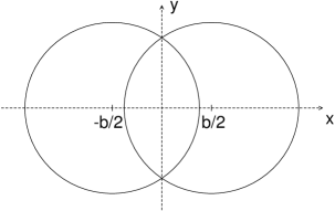
Figure 1: The transverse plane of a non-central $AA$ collision with the impact parameter $b$.

Usually, in the literature (see, e.g., Refs. Skokov_MC ; Deng_MC ; Liao_MC ; Roy_MC ) fluctuations of the electromagnetic fields in $AA$ collisions are treated using the classical Lienard-Weichert potentials of the protons within the Monte-Carlo simulation with the Woods-Saxon (WS) nuclear distributions. This approach gives rather large event-by-event fluctuations of the magnetic field (both parallel and perpendicular to the reaction plane). However, the classical Monte-Carlo treatment has no serious theoretical justification. The deviations from the classical approach may come both from the dynamical quantum effects in the colliding nuclei and from the quantum effects for the electromagnetic fields. Indeed, the field fluctuations should be most sensitive to the large scale fluctuation of the electric charge density in the colliding nuclei. It is well known that such large scale fluctuations in heavy nuclei are dominated by the collective giant resonances (see, e.g., Refs. BM ; Greiner ; Speth ; Roca ). From the point of view of fluctuations of the electromagnetic fields in heavy ion collisions the potentially important collective excitations are the isovector giant dipole resonance (IV-GDR) and isoscalar/isovector giant quadrupole resonances (IS/IV-GQRs) with the energy $\omega_{R}\sim 10-25$ MeV Speth ; Roca (the isoscalar modes correspond to the shape vibrations of the nucleus as a whole, and for the isovector ones protons and neutrons oscillate out of phase). But the factorized WS nuclear distribution ignores the collective quantum effects. From the side of the electromagnetic field the classical treatment should be invalid when the distance from the nucleus, $R$, in the nucleus rest frame, becomes bigger than $1/\omega_{R}$. Since for the central rapidity region (i.e. at $z$ close to zero in the center mass frame) $R\sim\tau\gamma$ (here $\tau$ is the proper time and $\gamma$ is the Lorentz factor), it means that the classical model fails already at the proper time $\tau\mathrel{\hbox to0.0pt{\lower 4.0pt\hbox{\hskip 1.0pt$\sim$}\hss}\raise 1.0pt\hbox{$>$}}0.1$ fm for RHIC energies and at $\tau\mathrel{\hbox to0.0pt{\lower 4.0pt\hbox{\hskip 1.0pt$\sim$}\hss}\raise 1.0pt\hbox{$>$}}0.01$ fm for LHC energies.

The quantum calculation of the electromagnetic field fluctuations in $AA$ collisions can be performed using the general formulas of the fluctuation-dissipation theorem (FDT) Callen for the electromagnetic fluctuations given in LL9 . In the case of interest the field fluctuations can be expressed via the nuclear dipole and quadruple polarizabilities. The contribution of the dipole mode have been addressed in Ref. Z1 . The results of this analysis show that in the quantum picture the field fluctuations turn out to be much smaller than predictions of the classical Monte-Carlo simulation with the WS nuclear density. It is highly desirable to perform the quantum calculation including the quadrupole modes. Although the contribution of the quadrupole modes decease steeper with $R$ than that for the dipole mode, they potentially may become important in the region of small proper time (which corresponds to small $R$), where the effects of the magnetic fields should be strongest. In the present letter we address the field fluctuations accounting for both the GDR and GQRs.

II Theoretical framework

We consider $AA$ collision between right moving and left moving nuclei with velocities ${{\bf V}}_{R}=(0,0,V)$ and ${{\bf V}}_{L}=(0,0,-V)$, and with the impact parameters ${{\bf b}}_{R}=(0,-b/2)$ and ${{\bf b}}_{L}=(0,b/2)$ (as shown in Fig. 1). We take $z_{R,L}=\pm Vt$. We evaluate the electromagnetic fields generated by two colliding nuclei in the ground state. As in Ref. Z1 , we ignore the electromagnetic fields generated by the induced currents in the QGP created after $AA$ collision. The total electromagnetic field is a sum of the fields generated by the colliding nuclei. For each nucleus, we write the electromagnetic field as a sum of the mean field and the fluctuating field

$$F^{\mu\nu}=\langle F^{\mu\nu}\rangle+\delta F^{\mu\nu}\,.$$ (1)

$\langle{{\bf E}}\rangle$ and $\langle{{\bf B}}\rangle$ are given by the Lorentz transformation of its Coulomb field in the nucleus rest frame. The mean magnetic field for two colliding nuclei at $\mbox{{\bf r}}=0$ has only $y$-component. Simple calculations give for the total mean $y$-component of the magnetic field at $t^{2}\mathrel{\hbox to0.0pt{\lower 4.0pt\hbox{\hskip 1.0pt$\sim$}\hss}\raise 1.0pt\hbox{$>$}}(R_{A}^{2}-b^{2}/4)/\gamma^{2}$ (here $R_{A}$ is the nucleus radius, and $b$ is assumed to be $<2R_{A}$)

$$\langle B_{y}(t,\mbox{{\bf r}}=0)\rangle\approx\frac{\gamma Zeb}{(b^{2}/4+\gamma^{2}V^{2}t^{2})^{3/2}}\,.$$ (2)

At $t\gg R_{A}/\gamma$ in the region $\rho\ll t\gamma$ $\langle B_{y}(t,\mbox{{\boldmath$\rho$}},z=0)\rangle$ takes a simple $\rho$-independent form

$$\langle B_{y}(t,\mbox{{\boldmath$\rho$}},z=0)\rangle\approx Zeb/\gamma^{2}t^{3}\,.$$ (3)

For each colliding nucleus, we first calculate the correlators of the fluctuating electromagnetic fields in the nucleus rest frame, and then perform the Lorentz transformation to the center of mass lab-frame of $AA$ collision. We use the FDT formalism for electromagnetic fluctuations of LL9 , formulated in the gauge $\delta A^{0}=0$. It relates the time Fourier component of the vector potential correlator

$$\langle\delta A_{i}(\mbox{{\bf r}}_{1})\delta A_{k}(\mbox{{\bf r}}_{2})\rangle_{\omega}=\frac{1}{2}\int dte^{i\omega t}\langle\delta A_{i}(t,\mbox{{\bf r}}_{1})\delta A_{k}(0,\mbox{{\bf r}}_{2})$$

$$+\delta A_{k}(0,\mbox{{\bf r}}_{2})\delta A_{i}(t,\mbox{{\bf r}}_{1})\rangle\hskip 56.9055pt$$ (4)

to the retarded Green function

$$D_{ik}(\omega,\mbox{{\bf r}}_{1},\mbox{{\bf r}}_{2})=-i\int dte^{i\omega t}\theta(t)\langle\delta A_{i}(t,\mbox{{\bf r}}_{1})\delta A_{k}(0,\mbox{{\bf r}}_{2})$$

$$-\delta A_{k}(0,\mbox{{\bf r}}_{2})A_{i}(t,\mbox{{\bf r}}_{1})\rangle\,.\hskip 56.9055pt$$ (5)

For the case of the zero temperature, that we need, the FDT relation between (4) and (5) reads LL9

$$\!\!\langle\delta A_{i}(\mbox{{\bf r}}_{1})\delta A_{k}(\mbox{{\bf r}}_{2})\rangle_{\omega}\!=\!-\mbox{sign}(\omega)\mbox{Im}D_{ik}(\omega,\mbox{{\bf r}}_{1},\mbox{{\bf r}}_{2}).$$ (6)

In vacuum the Green function is given by LL9

$$D_{ik}^{v}(\omega,\mbox{{\bf r}}_{1},\mbox{{\bf r}}_{2})=\delta_{ik}D_{1}(\omega,r)+\frac{x_{i}x_{k}}{r^{2}}D_{2}(\omega,r)\,,$$ (7)

where $\mbox{{\bf r}}=\mbox{{\bf r}}_{1}-\mbox{{\bf r}}_{2}$, and

$$D_{1}(\omega,r)=-\frac{e^{i\omega r}}{r}\left(1+\frac{i}{\omega r}-\frac{1}{\omega^{2}r^{2}}\right)\,,$$ (8)

$$D_{2}(\omega,r)=\frac{e^{i\omega r}}{r}\left(1+\frac{3i}{\omega r}-\frac{3}{\omega^{2}r^{2}}\right)\,.$$ (9)

The vacuum Green function corresponds to the ordinary vacuum fluctuations of electromagnetic fields. For our purpose in this work, we need only correction to the vacuum Green function at $\mbox{{\bf r}}_{1}=\mbox{{\bf r}}_{2}$ due to interaction of electromagnetic fields with the nuclei. We calculate it assuming that $R=|\mbox{{\bf r}}_{1,2}-\mbox{{\bf r}}_{A}|$ is large as compared to the nucleus radius $R_{A}$, when the nucleus can be treated as a point-like object described by the nucleus polarizability tensors. In the present analysis we account for the effect of the dipole and quadrupole nucleus modes. The dipole contribution to $\Delta D_{ik}$ can written as LL9

$$\Delta D_{ik}^{d}(\omega,\mbox{{\bf r}}_{1},\mbox{{\bf r}}_{2})=-\omega^{2}D_{il}^{v}(\omega,\mbox{{\bf r}}_{1},\mbox{{\bf r}}_{A})\alpha_{lm}(\omega)$$

$$\times D_{mk}^{v}(\omega,\mbox{{\bf r}}_{A},\mbox{{\bf r}}_{2})\,.$$ (10)

where $\alpha_{ik}(\omega)$ is the dipole nuclear polarizability tensor. The tensor $\alpha_{ik}(\omega)$ can be written as LL4 ; Migdal_GDR

$$\alpha_{ik}(\omega)=\sum_{s}\left[\frac{\langle 0|{{\bf d}}_{i}|s\rangle\langle s|{{\bf d}}_{k}|0\rangle}{\omega_{s0}-\omega-i\delta}+\frac{\langle 0|{{\bf d}}_{k}|s\rangle\langle s|{{\bf d}}_{i}|0\rangle}{\omega_{s0}+\omega+i\delta}\right]\,,$$ (11)

where ${{\bf d}}$ is the dipole operator. The formulas (10), (11) correspond to the dipole approximation of the electromagnetic interaction operator $V=-{{\bf d}}{{\bf E}}$ LL4 . For the quadrupole excitations the electromagnetic interaction operator reads $V=-\frac{1}{6}\sum_{i,j}Q_{ij}\frac{\partial E_{i}}{\partial x_{j}}$ LL2 ; Greiner_PR151 , where $Q_{ij}$ is the operator of the quadrupole moment. And the quadrupole counterpart of the dipole contribution to $\Delta D_{ik}$ (10) can be written as

$$\Delta D_{ik}^{q}(\omega,\mbox{{\bf r}}_{1},\mbox{{\bf r}}_{2})=-\omega^{2}\frac{\partial}{\partial\mbox{{\bf r}}_{A}^{j}}D_{il}^{v}(\omega,\mbox{{\bf r}}_{1},\mbox{{\bf r}}_{A})\alpha_{ljmn}(\omega)$$

$$\times\frac{\partial}{\partial\mbox{{\bf r}}_{A}^{n}}D_{mk}^{v}(\omega,\mbox{{\bf r}}_{A},\mbox{{\bf r}}_{2})\,,$$ (12)

where now $\alpha_{ljmn}(\omega)$ is the quadrupole nuclear polarizability tensor. The quadrupole counterpart of the representation (11) for the dipole tensor $\alpha_{ik}(\omega)$ is given by

$$\alpha_{ijmn}(\omega)=\frac{1}{6^{2}}\sum_{s}\left[\frac{\langle 0|Q_{ij}|s\rangle\langle s|Q_{mn}|0\rangle}{\omega_{s0}-\omega-i\delta}\right.$$

$$+\left.\frac{\langle 0|Q_{mn}|s\rangle\langle s|Q_{ij}|0\rangle}{\omega_{s0}+\omega+i\delta}\right]\,.$$ (13)

The formulas (10), (12) correspond to the approximation of a point-like nucleus with the dipole and quadrupole moments. Note that the applicability condition $R/R_{A}\gg 1$ (here, as above, $R=|\mbox{{\bf r}}_{1,2}-\mbox{{\bf r}}_{A}|$ is the distance from the observation point at $\mbox{{\bf r}}_{1}=\mbox{{\bf r}}_{2}$ to the center of the nucleus in its rest frame) for this approximation means that the time $t$ in the center of mass lab-frame of $AA$ collision for the center of the QGP fireball must be large as compared to $R_{A}/\gamma$.

The field correlators that we need can be written as

$$\langle\delta E_{i}(t,\mbox{{\bf r}})\delta E_{k}(t,\mbox{{\bf r}})\rangle=\frac{1}{2\pi}\int_{-\infty}^{\infty}d\omega\langle\delta E_{i}(\mbox{{\bf r}})\delta E_{k}(\mbox{{\bf r}})\rangle_{\omega}\,,$$ (14)

$$\langle\delta B_{i}(t,\mbox{{\bf r}})\delta B_{k}(t,\mbox{{\bf r}})\rangle=\frac{1}{2\pi}\int_{-\infty}^{\infty}d\omega\langle\delta B_{i}(\mbox{{\bf r}})\delta B_{k}(\mbox{{\bf r}})\rangle_{\omega}\,.$$ (15)

Here the time Fourier components of the electromagnetic field correlators in terms of that for the the vector potential correlator (4) are given by

$$\langle\delta E_{i}(\mbox{{\bf r}}_{1})\delta E_{k}(\mbox{{\bf r}}_{2})\rangle_{\omega}=\omega^{2}\langle\delta A_{i}(\mbox{{\bf r}}_{1})\delta A_{k}(\mbox{{\bf r}}_{2})\rangle_{\omega}\,,$$ (16)

$$\langle\delta B_{i}(\mbox{{\bf r}}_{1})\delta B_{k}(\mbox{{\bf r}}_{2})\rangle_{\omega}=\mbox{rot}^{(1)}_{il}\mbox{rot}^{(2)}_{kj}\langle\delta A_{l}(\mbox{{\bf r}}_{1})\delta A_{j}(\mbox{{\bf r}}_{2})\rangle_{\omega},$$ (17)

where the vector potential correlator should be calculated using (6) with replacement of the full tensor $D_{ik}$ by the correction $\Delta D_{ik}$ due to interaction of the electromagnetic field with the dipole (10) and quadrupole (12) modes.

We will consider the spherically symmetrical even-even ²⁰⁸Pb nucleus. In this case the dipole and quadrupole polarization tensors can be written in terms of two scalar functions $\alpha_{d}=\alpha_{ii}$ and $\alpha_{q}=\alpha_{ijij}$ as

$$\alpha_{ij}=\alpha_{d}\delta_{ik}/3\,,$$ (18)

$$\alpha_{ijkl}=\frac{1}{10}\alpha_{q}\left[\delta_{ik}\delta_{jl}+\delta_{il}\delta_{jk}-\frac{2}{3}\delta_{ij}\delta_{kl}\right]\,.$$ (19)

The relation (19) can be obtained using the fact that the quadrupole operator satisfies the relation $Q_{ii}=0$. It is important that $\alpha_{d}$ and $\alpha_{q}$ are analytical functions of $\omega$ in the upper half-plane LL4 , and satisfy the relation $\alpha^{*}(-\omega^{*})=\alpha(\omega)$ LL4 . It allows, for both the modes, to transform the integrals over $\omega$ in (14), (15) from $-\infty$ to $\infty$ to those along the positive imaginary axis, where $\alpha_{d,q}$ are real.

We parametrize the functions $\alpha_{d,q}$ by a single Lorentzian form

$$\alpha_{i}(\omega)=c_{i}\left[\frac{1}{\omega_{i}-\omega-i\Gamma_{i}/2}+\frac{1}{\omega_{i}+\omega+i\Gamma_{i}/2}\right]\,.$$ (20)

The imaginary part of the polarizability is proportional to the photoabsorption cross section LL4 ; Greiner_PR151 . The GDR for ²⁰⁸Pb due to $E1$ transition is well seen in the data on the photoabsorption cross section GDR_Pb . In Ref. Z1 by fitting the photoabsorption cross section for ²⁰⁸Pb from Ref. GDR_Pb we obtained for the dipole mode: $\omega_{d}\approx 13.3$ MeV, $\Gamma_{d}\approx 3.72$ MeV, and $c_{d}\approx 56.79$ Gev^-3. For the quadrupole case we include both the IS-GQR and the IV-GQR. The contributions of the GQRs to the photoabsorption cross section due to the IS and IV $E2$ transitions are much smaller than that from the GDR due to the $E1$ transition Roca . It renders difficult an accurate fit of the parameters of the GQRs from data on the photoabsoption cross section. We use parameters of the IS-GQR obtained in Ref. IS1 from measurements of the IS $E2$ strength in inelastic scattering of $\alpha$ particles at small angles: $\omega_{q}^{IS}\approx 10.89$ MeV and $\Gamma_{q}^{IS}\approx 3$ MeV. We extracted the normalization constant from the energy weighted sum rule (EWSR) (see, e.g., Refs. Speth ; Roca ) for the isoscalar quadrupole moment that to a good accuracy is exhausted by the IS-GQR IS1 . This gives $c_{q}^{IS}\approx 3984$ Gev^-5. For the IV-GQR we use parameters obtained in the recent most accurate measurement IV1 via polarized Compton scattering: $\omega_{q}^{IV}\approx 23$ MeV and $\Gamma_{q}^{IV}\approx 3.9$ MeV. For the IV modes the EWSR may be violated by $\sim 20-30$% due to the exchange potential in the nuclear Hamiltonian RMP63 ; Migdal_GDR ; Roca . The experimental data from Refs. IV1 ; IV19 ; IV20 ; IV11 give the exhaustion of the IV EWSR $100\pm 40$%. We use the result of the most accurate measurement IV1 , that gives the exhaustion of the IV EWSR $56\pm 5$%. This leads to the normalization constant for the IV quadrupole polarizability $c_{q}^{IV}\approx 1524$ Gev^-5. The possible errors in the $c_{q}^{IV}$ are not very important because anyway the IV contribution turns out to be suppressed as compared to the IS one due to bigger energy of the IV-GQR.

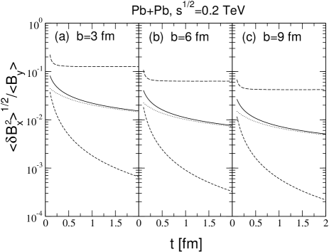
Figure 2: Ratio $\langle\delta B_{x}^{2}\rangle^{1/2}/\langle B_{y}\rangle$ versus $t$ at $\mbox{{\bf r}}=0$ for Pb+Pb collisions at $\sqrt{s}=0.2$ TeV for impact parameters $b=3$, $6$ and $9$ fm. Results of quantum calculations: solid line is for the total contribution of the GDR, IS-GQR and IV-GQR, dotted line is for the contribution of the GDR, dashed line is for sum of the contributions of the IS-GQR and IV-GQR. Long-dashed lines show results of the classical Monte-Carlo calculation with the WS nuclear density.

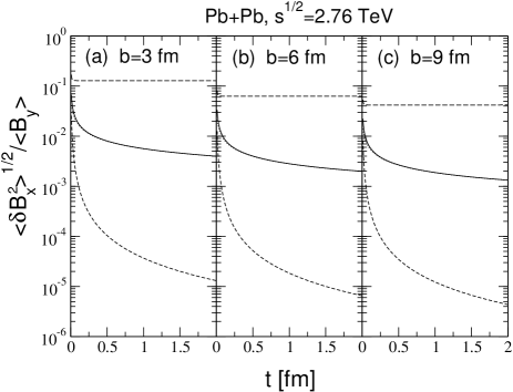
Figure 3: Same as in Fig. 2 but for $\sqrt{s}=2.76$ TeV.

III Numerical results

For applications the most interesting effect of the field fluctuation is fluctuation of the direction of the magnetic field at the center of the plasma fireball. It is dominated by the fluctuations of the component $B_{x}$ that vanishes without field fluctuations. In Figs. 2, 3 we show our results for $t$-dependence of the ratio $\langle\delta B_{x}^{2}\rangle^{1/2}/\langle B_{y}\rangle$ (which gives the typical angle between the magnetic field and the perpendicular to the reaction plane) at $\mbox{{\bf r}}=0$ for the impact parameters $b=3,$ $6$ and $9$ fm for RHIC energy $\sqrt{s}=0.2$ and LHC energy $\sqrt{s}=2.76$ TeV. For comparison we also show predictions of the classical Monte-Carlo calculations for the WS nuclear density. We present the results for $t_{min}<t<2$ fm with $t_{min}=0.1(0.01)$ fm for $\sqrt{s}=0.2(2.76)$ TeV. This values of $t_{min}$, in terms of the equations (10) and (12), correspond to the situation with $|\mbox{{\bf r}}_{1,2}-\mbox{{\bf r}}_{A}|/R_{A}\mathrel{\hbox to0.0pt{\lower 4.0pt\hbox{\hskip 1.0pt$\sim$}\hss}\raise 1.0pt\hbox{$>$}}2-3$, when the observation point is still not too close to the nuclei (in their rest frames). In this case even at minimal $t$ the approximation of the point-like nuclei should still be reasonable. Figs. 2, 3 show that at $t\sim t_{min}$ in the quantum picture $\langle\delta B_{x}^{2}\rangle^{1/2}/\langle B_{y}\rangle$ is smaller than in the classical one by a factor of $\sim 3$. One can see that at $t\sim t_{min}$ in the quantum picture the quadrupole contribution is of the order of the dipole one. But the relative contribution of the GQRs falls steeply with increase of $t$. And it becomes very small at $t\mathrel{\hbox to0.0pt{\lower 4.0pt\hbox{\hskip 1.0pt$\sim$}\hss}\raise 1.0pt\hbox{$>$}}0.5(0.05)$ fm for $\sqrt{s}=0.2(2.76)$ TeV. In this region the quantum picture gives $\langle\delta B_{x}^{2}\rangle^{1/2}/\langle B_{y}\rangle$ that is smaller than the classical prediction by a factor of $\sim 3-8$ for $\sqrt{s}=0.2$ TeV and by a factor of $\sim 6-30$ for for $\sqrt{s}=2.76$ TeV. Note that the quadrupole contribution comes mostly from the IS mode that has a smaller excitation energy. The field fluctuations also lead to nonzero values of the transverse electric field $\langle\delta E_{x,y}^{2}\rangle^{1/2}$ at $\mbox{{\bf r}}=0$, that vanishes for the average field. The results for $\langle\delta E_{x,y}^{2}\rangle^{1/2}$ at $\mbox{{\bf r}}=0$ are very similar to that for magnetic field.

Thus we see that in the quantum picture fluctuations of the direction of the magnetic field relative to the reaction plane turns out to be considerably smaller than in the classical picture. The reduction of the field fluctuations in the quantum picture comes partly from smaller fluctuations of the dipole and quadrupole moments and partly from the dynamical quantum effects in the electromagnetic fields. The latter lead to an increase of the difference between the quantum and the classical models with increasing $t$. This quantum effects for the electromagnetic fields become important in the regime when $R=|\mbox{{\bf r}}_{1,2}-\mbox{{\bf r}}_{A}|$ in (10), (12) is large as compared to the inverse giant resonance excitation energies. The reduction of the fluctuations of the dipole and quadrupole moments in the quantum picture can be demonstrated by comparing the $\langle 0|{{\bf d}}^{2}|0\rangle$ and $\langle 0|(Q_{ij}/6)^{2}|0\rangle$ with their classical counterparts predicted by the Monte-Carlo calculations with the WS nuclear density. In quantum picture the dipole moment squared can be written as Z1

$$\langle 0|{{\bf d}}^{2}|0\rangle=\frac{1}{\pi}\int_{0}^{\infty}d\omega\mbox{Im}\alpha_{d}(\omega)\,.$$ (21)

It gives a value by a factor of $\sim 5$ smaller than the prediction of the classical Monte-Carlo calculation with the WS nuclear density. For the quadrupole mode one can easily obtain from (13), (19) a similar formula

$$\langle 0|(Q_{ij}/6)^{2}|0\rangle=\frac{1}{\pi}\int_{0}^{\infty}d\omega\mbox{Im}\alpha_{q}(\omega)\,.$$ (22)

Calculations using this formula show that the quantum result is smaller than prediction of the classical Monte-Carlo calculation with the WS nuclear density by a factor of $\sim 8$. The fact the classical treatment based on the WS nuclear density overestimates the fluctuations of the dipole and quadrupole moments means that it overestimates the ellipsoidal fluctuations of the nuclear density. Note that this may be very important for the event-by-event hydrodynamic simulations of $AA$ collision that presently ignore possible collective effects in the nuclear distributions.

IV Conclusion

In this work we have performed a quantum analysis of fluctuations of the electromagnetic field in $AA$ collisions at RHIC and LHC energies. We use the FDT formalism of LL9 accounting for the contributions to the nucleus polarizability of the dipole and quadrupole modes. We have found that for each nucleus the contribution of the IS and IV quadrupole modes is of the order of that of the dipole mode when the distance between the observation point and the center of the nucleus in the nucleus rest frame is $\sim 2R_{A}$. For the center of the QGP fireball in the center mass frame of $AA$ collisions it corresponds to time $t\sim 0.1(0.01)$ fm for RHIC(LHC) energy, and at $t\mathrel{\hbox to0.0pt{\lower 4.0pt\hbox{\hskip 1.0pt$\sim$}\hss}\raise 1.0pt\hbox{$>$}}0.5(0.05)$ fm the dipole mode dominates the field fluctuations.

Our quantum calculations show that effect of the field fluctuations is considerably smaller than that in the classical Monte-Carlo simulation with the WS nuclear distribution. And in the quantum picture the fluctuations of the direction of the magnetic field as compared to the mean field turn out to be very small. Our results do not support a qualitative analysis Tuchin_quantum , where it was argued that the quantum diffusion of the protons may be very important.

In the present analysis we have discussed the case of the spherical ²⁰⁸Pb nucleus. For collisions of the deformed ¹⁹⁷Au nuclei, that have been studied in RHIC experiments, one should account for a non-zero mean quadrupole moment. This can modify the contribution of the quadrupole fluctuations. But the magnitude of the quantum quadrupole fluctuation around the equilibrium shape for the deformed nuclei is similar to that for spherical ones (see, e.g., Refs. Scamps1 ; Scamps2 ). Since the GDR peak in the photoabsorption cross section for ¹⁹⁷Au GDR_Au is very similar to that for the ²⁰⁸Pb nucleus GDR_Pb , the dominating contributions of the GDR to the field fluctuations for these nuclei are also similar. For this reason the conclusion that the classical approach overestimates the field fluctuations should hold for Au+Au collisions as well.

- (1) D.E. Kharzeev, L.D. McLerran, and H.J. Warringa, Nucl. Phys. A803, 227 (2008) [arXiv:0711.0950].
- (2) V. Skokov, A.Yu. Illarionov, and V. Toneev, Int. J. Mod. Phys. A24, 5925 (2009) [arXiv:0907.1396].
- (3) K. Tuchin, Phys. Rev. C88, 024911 (2013) [arXiv:1305.5806].
- (4) B.G. Zakharov, Phys. Lett. B737, 262 (2014) [arXiv:1404.5047].
- (5) D.E. Kharzeev, Prog. Part. Nucl. Phys. 75, 133 (2014) [arXiv:1312.3348].
- (6) K. Tuchin, Phys. Rev. C91, 014902 (2015) [arXiv:1406.5097].
- (7) B.G. Zakharov, Eur. Phys.J. C76, 609 (2016) [arXiv:1609.04324].
- (8) K. Fukushima, K. Hattori, and Y. Yin, Phys. Rev. D93, 074028 (2016) [arXiv:1512.03689].
- (9) S.I. Finazzo, R. Critelli, R. Rougemont, and J. Noronha, Phys. Rev. D94, 054020 (2016) [Erratum-ibid. D96, 019903 (2017)] [arXiv:1605.06061].
- (10) V. Roy, S. Pu, L. Rezzolla, and D.H. Rischke, Phys.Rev. C96, 054909 (2017) [arXiv:1706.05326].
- (11) A. Das, S.S. Dave, P.S. Saumia, and A.M. Srivastava, Phys.Rev. C96, 034902 (2017), [arXiv:1703.08162].
- (12) V. Roy, Universe 3, 82 (2017).
- (13) L. McLerran and V. Skokov, Nucl. Phys. A929, 184 (2014) [arXiv:1305.0774].
- (14) J. Bloczynski, X.-G. Huang, X. Zhang, and J. Liao, Phys. Lett. B718, 1529 (2013) [arXiv:1209.6594].
- (15) A. Bzdak and V. Skokov, Phys. Lett. B710, 171 (2012) [arXiv:1111.1949].
- (16) W.-T. Deng and X.-G. Huang, Phys. Rev. C85, 044907 (2012) [arXiv:1201.5108].
- (17) V. Roy and S. Pu, Phys.Rev. C92, 064902 (2015) [arXiv:1508.03761].
- (18) A. Bohr and B.R. Mottelson, Nuclear structure, vol. I & II. W.A. Benjamin, Inc., 1975.
- (19) W. Greiner and J.A. Maruhn, Nuclear models, Berlin, Springer, 1996.
- (20) S. Kamerdzhiev, J. Speth, and G. Tertychny, Phys. Rept. 393, 1 (2004) [nucl-th/0311058].
- (21) X. Roca-Maza and N. Paar, Prog. Part. Nucl. Phys. 101, 96 (2018) [1804.06256].
- (22) H.B. Callen and T.A. Welton, Phys. Rev. 83, 34 (1951).
- (23) E.M. Lifshits and L.P. Pitaevski, Statistical Physics, Part 2 (Landau Course of Theoretical Physics Vol. 9), Oxford, Pergamon Press, 1980.
- (24) B.G. Zakharov, JETP Lett. 105, 758 (2017) [arXiv:1703.04271].
- (25) V.B. Berestetski, E.M. Lifshits, and L.P. Pitaevski, Quantum Electrodynamics (Landau Course of Theoretical Physics Vol. 4), Oxford, Pergamon Press, 1979.
- (26) A.B. Migdal, A.A. Lushnikov, and D.F. Zaretsky, Nucl. Phys. 66, 193 (1965).
- (27) L.D. Landau and E.M. Lifshitz, Classical Theory of Fields, Butterworth-Heinemann, Oxford, UK, 1987.
- (28) M. Danos, W. Greiner, and C.B. Kohr, Phys. Rev. 151, 761 (1966).
- (29) A. Tamii et al., Phys. Rev. Lett. 107, 062502 (2011) [arXiv:1104.5431].
- (30) D.H. Youngblood, Y.W. Lui, H.L. Clark, B. John, Y. Tokimoto, and X. Chen Phys. Rev. C69, 034315 (2004).
- (31) S.S. Henshaw, M.W. Ahmed, G. Feldman, A.M. Nathan, and H.R. Weller, Phys. Rev. Lett. 107, 222501 (2011).
- (32) E. Hayward, Rev. Mod. Phys. 35, 324 (1963).
- (33) R. Leicht, M. Hammen, K.P. Schelhaas, and B. Ziegler, Nucl. Phys. A362, 111 (1981).
- (34) K.P. Schelhaas, J.M. Henneberg, M. Sanzone-Arenhövel, N. Wieloch-Laufenberg, U. Zurmühl, B. Ziegler, M. Schumacher, and F. Wolf. Nucl. Phys. A489, 189 (1988).
- (35) D.S. Dale, R.M. Laszewski, and R. Alarcon, Phys. Rev. Lett. 68, 3507(1992).
- (36) R. Holliday, R. McCarty, B. Peroutka, and K. Tuchin, Nucl. Phys. A957, 406 (2017) [arXiv:1604.04572].
- (37) G. Scamps and D. Lacroix, Phys. Rev. C88, 044310 (2013) [arXiv:1307.1909].
- (38) G. Scamps and D. Lacroix, Phys. Rev. C89, 034314 (2014) [arXiv:1401.5211].
- (39) A. Veyssiere, H. Beil, R. Bergere, P. Carlos, and A. Lepretre, Nucl. Phys. A159, 561 (1970).