An Analytical Solution to the $k$-core Pruning Process

Abstract

$k$-core decomposition is widely used to identify the center of a large network, it is a pruning process in which the nodes with degrees less than $k$ are recursively removed. Although the simplicity and effectiveness of this method facilitate its implementation on broad applications across many scientific fields, it produces few analytical results. We here simplify the existing theoretical framework to a simple iterative relationship and obtain the exact analytical solutions of the $k$-core pruning process on large uncorrelated networks. From these solutions we obtain such statistical properties as the degree distribution and the size of the remaining subgraph in each of the pruning steps. Our theoretical results resolve the long-lasting puzzle of the $k$-core pruning dynamics and provide an intuitive description of the dynamic process.

Introduction

In the k-core pruning process we recursively remove the nodes with degrees less than $k$. We iteratively repeat the process until a finite-sized subgraph, the $k$-core of the network, is obtained. If it is not obtained, the network disappears. Fig. 1 shows a simplified picture of $k$-core decomposition. Note that a $2$-core decomposition is performed on the network, and that the final $2$-core is obtained in step 3 (Fig. 1d).

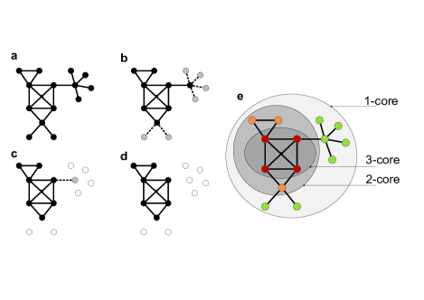
Figure 1: The illustration of $k$-core pruning process and $k$-core. a-d, the detailed pruning steps of $2$-core, the discs represent nodes and the solid lines indicate the links. Grey discs and dashed lines represent the nodes and links that will be removed in this step. Dashed circles stand for the nodes that have been removed. a)The starting network. b)The first pruning step, remove the nodes with degrees less than $2$, and links incident to them. Note after this step, the node in the top right corner that previously had degree of $5$ will be left with only one link. c)The second pruning step, remove the nodes whose degree is fewer than $2$. d)The final step. All nodes remained in the network have more than $2$ links, and the iterative process terminates in this step. e)$k$-core decomposition result of the network. $1$-core contains all the nodes, so it is trivial. $2$-core contains the nodes marked with red and orange, and $3$-core of the network contains the red nodes.

The first proposed application of $k$-core decomposition was to measure the centrality of nodes in a network Seidman (1983), but more recently it has been applied to many disciplines, including biology, informatics, economy, and network science. Bader et al. Bader and Hogue (2003) developed an algorithm based on $k$-core decomposition to identify the densely linked regions in the protein-protein interaction (PPI) network, which may represent molecular complexes. Altaf et al.  Altaf-Ul-Amine et al. (2003) use the k-core decomposition to predict the PPI functions of several function-unknown proteins. Stefan Wuchty et al. Wuchty and Almaas (2005) discovered that the probability of proteins being essential and conserved through stages of evolution increases with the $k$-coreness of the protein. Nir Lahav et al. Lahav et al. (2016) used $k$-core decomposition to describe the hierarchical structure of the cortical organization in the human brain. They discovered that the strongest hierarchy serves as a platform for the emergence of consciousness. Researchers in information science, economics, and complex networks have also used $k$-core as a filter to obtain relevant information in a large system Gaertler and Patrignani (2004); Carmi et al. (2007), to identify the central countries during economic crises Garas et al. (2010), to locate the most influential propagators in a complex network system Kitsak et al. (2010); Morone and Makse (2015), and to predict structural collapse in mutualistic ecosystems Morone et al. (2019).

Because $k$-core decomposition has so many applications, researchers Fernholz and Ramachandran (2004); Dorogovtsev et al. (2006) have used theoretical analyses and numerical simulations to study the final state of $k$-core decomposition and have found that a giant $k$-core emerges in the form of a phase transition Dorogovtsev et al. (2008). The $k$-core exists only when the initial average degree of nodes is above a critical point, denoted $c^{*}$. Baxter et al. Baxter et al. (2015) propose a theoretical framework of four equations to describe the evolution of the degree distribution. Their numerical calculation on Erdős-Rényi networks when $k=3$ show that a long-lasting transient “plateau” stage exists before the final collapse when the initial mean degree is close to the critical value.

Although the numerical result reveals that the $k$-core pruning process has many interesting properties, the analytical result is still hindered by its mathematical difficulty Baxter et al. (2015). In this paper we correct an oversight in the previous research Baxter et al. (2015) in which the probability cannot be normalized because it is missing a non-negligible term in its original theoretical framework. More important, we solve the mathematical problem by inducing an auxiliary series and obtaining the analytical solution for any large uncorrelated network. Our results clearly describe the subgraph in each pruning step and agree with various numerical simulations.

To analyze of $k$-core decomposition theoretically we need to determine how many nodes remain in the network after each pruning process and discover the structural topology, i.e., the degree distribution, of the subgraph. We here present complete results for both. We begin with a brief introduction of the theoretical framework given in Ref. Baxter et al. (2015).

In each step of the $k$-core pruning process on a large uncorrelated network with a finite average degree, we remove nodes with a degree less than $k$. For convenience we assume that pruned nodes remain in the network, but are with degrees equal to zero. We denote the $n^{th}$ network after pruning $n$ by $\mathcal{N}_{n}$, and designate $G_{n,0}(z)=\sum_{j=0}^{\infty}p_{n,j}z^{j}$—the notation supplied in Ref. Newman (2018)—to be the probability generating function for the degree distribution of $\mathcal{N}_{n}$, where $p_{n,j}$ is the degree distribution in $\mathcal{N}_{n}$. Similarly $G_{n,1}(z)=\sum_{j=0}^{\infty}q_{n,j}z^{j}$ is the probability generating function for the excess degree distribution of $\mathcal{N}_{n}$, where $q_{n,j}$ is the excess degree distribution, i.e., the degree distribution of a node reached by following a randomly chosen link, excluding the chosen link itself. We simplify the notation of initial generating functions from $G_{0,0}$ and $G_{0,1}$ to $G_{0}$ and $G_{1}$, respectively.

In pruning process $n$ on network $\mathcal{N}_{n-1}$ (see SI 1A for a schematic illustration), $v_{n-1}$ is the probability that when we randomly follow a link to one node in $\mathcal{N}_{n-1}$ it has a degree greater than $k-2$,

$$v_{n-1}=1-\sum_{j=0}^{k-2}q_{n-1,j}.$$ (1)

Here the set of nodes with a degree equal to $0$ after $k$-core pruning $n$ has (i) nodes with a degree less than $k$ and (ii) nodes with degrees not less than $k$ but with neighbors all having degrees less than $k$. Note that in previous research Baxter et al. (2015) this latter term was missing,

$$p_{n,0}=\sum_{j=0}^{k-1}p_{n-1,j}+\sum_{j=k}^{\infty}p_{n-1,j}(1-v_{n-1})^{j}.$$ (2)

Nodes that have degree $i$ after pruning $n$ have degree $j$, which is never less than $max\{i,k\}$, and $j-i$ neighbors are removed after pruning $n$,

$$p_{n,i}=\sum_{j=max\{i,k\}}^{\infty}p_{n-1,j}{j\choose i}v_{n-1}^{i}(1-v_{n-1})^{j-i}.$$ (3)

And the relationship between the degree distribution and the excess degree distribution after pruning $n$ is:

$$q_{n,i}=\frac{(i+1)p_{n,i+1}}{\sum_{i=0}^{\infty}ip_{n,i}}.$$ (4)

Although the theoretical framework for the four degree distribution evolution equations was first proposed by Baxter et al. Baxter et al. (2015), they noted that they were “difficult to study analytically” and solved them “numerically for Erdős-Rényi networks (Poisson degree distributions) using the initial mean degree $\langle q\rangle$ as a control parameter.” To obtain the result, one must use the degree distribution of the subgraph after the last pruning as an input, which is an infinite-dimensional vector when the network is large.In what follows, by introducing an auxiliary series $y_{n}$ we can simplify the complex infinite-dimensional simultaneous recurrence equations and make it an equivalent univariable iteration process. Then the relevant quantities, e.g., the size of the remaining subgraph $S_{n}$ in step $n$, can be obtained and expressed as a simple function of $y_{n}$.

First, we obtain the recurrence relation of $G_{n,0}(z)$ from (2), and (3) (see SI 1B for detail),

$$G_{n,0}(z)= G_{n-1,0}(1-v_{n-1}+zv_{n-1})$$ (5)

$$+\sum_{j=0}^{k-1}p_{n-1,j}(1-(1-v_{n-1}+zv_{n-1})^{j}).$$

To acquire the general form of $G_{n,0}$, we introduce an important auxiliary series,

$$y_{0} =1,$$ (6)

$$y_{n} =1-\sum_{j=0}^{k-2}\frac{y_{n-1}^{j}}{j!}G_{1}^{(j)}(1-y_{n-1})\equiv f(y_{n-1}).$$ (7)

Here $G^{(j)}(z)$ is derivative $j$ of $G(z)$, i.e., $G^{(j)}(z)=d^{j}G(z)/dz^{j}$. Then by induction we have the generating function(see SI 1C for detail)

$$G_{n,0}(z)=G_{0}(1-y_{n}+y_{n}z)$$

$$+\sum_{j=0}^{k-1}\frac{G_{0}^{(j)}(1-y_{n-1})}{j!}(y_{n-1}^{j}-(y_{n-1}-y_{n}+y_{n}z)^{j}).$$ (8)

The remaining subgraph after pruning $n$ have degrees no less than $k$ in the $\mathcal{N}_{n-1}$ network. Thus the size of the remaining subgraph $S_{n}$ after pruning $n$ is

$$S_{n}=\sum_{j=k}^{\infty}p_{n-1,j}=1-\sum_{j=0}^{k-1}\frac{G_{0}^{(j)}(1-y_{n-1})}{j!}y_{n-1}^{j}\equiv g(y_{n-1}).$$ (9)

Note that $S=\lim_{n\rightarrow\infty}S_{n}=g(y)$ is the size of the final $k$-core, and that $y$ is the largest root of $y=f(y)$ in $[0,1)$. This result is consistent with previous research Fernholz and Ramachandran (2004).

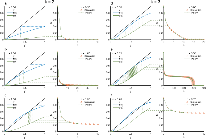
Figure 2: An illustration for the size of remaining subgraph $S_{n}$ in $k$-core pruning process performed on ER-networks. All panels consist of two panels, left and right. The left panels show $g(y)$ and the iteration of $y_{n}=f(y_{n-1})$ during the pruning process and the right panels show $S_{n}$ from both the theoretical result and numerical simulation result. The green dashed lines in between are indications of the corresponding relationship of $S_{n}=g(y_{n-1})$ according to our analytical result. a-c), the result of $2$-core pruning process below, at, and above the critical point $c^{*}=1$, respectively. d-f), the result of $3$-core pruning process below, near, and above the critical point $c^{*}=3.3509$, respectively. For a,b,c,d,f, the numerical results are obtained from simulations on $10^{6}$ nodes. Since the result is very sensitive to the random perturbation of the original network near the discontinuous phase transition point, the numerical result in e is averaged over 10 simulations on $5\times 10^{8}$ nodes.

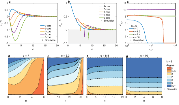
Figure 3: The structural properties of remaining subgraph of $k$-core decomposition on ER-network. The solid lines indicate the theoretical result and the circles represent the simulation result. a), the average degree change after the first step of pruning $c_{1}-c$ versus the initial average degree $c$. b), the difference between initial average degree and the average degree of $k$-core, denoted by $c_{\infty}-c$, versus the initial average degree $c$. c), The average degree evolution in each step of the $6$-core pruning process. Note that the horizontal axis is in logarithmic scale, and we shift $n^{th}$ step to $(n+1)^{th}$ step in order to show the data of initial condition ($n=0$). d-g), the stacked area chart of the nodes with different degrees, evolves with pruning steps. Here simulations of $6$-core decomposition are performed on $4$ random ER-networks with different initial average degrees, the results are shown in d-g, respectively. The networks have $10^{6}$ nodes except in e), the network has $10^{8}$ nodes.

From the exact expression of $S_{n}$ and $y_{n}$, we know that the computation of $y_{n}$ is equivalent to a fixed-point iteration and that $S_{n}$ can then be solved because it is a function of $y_{n-1}$. For 2-core decomposition on an ER-network, we obtain $f(y)=1-e^{-cy}$, $g(y)=1-e^{-cy}(1+cy)$. Thus each step of the pruning process can be represented by a corresponding iterative step of $y=f(y)$. Fig. 2 shows the process using a simple visualization method.

In 3-core decomposition, it is easy to acquire $f(y)=1-e^{-cy}(1+cy)$ and $g(y)=1-e^{-cy}(1+cy+(cy)^{2}/2)$. Unlike the result from 2-core decomposition, there is a discontinuous phase transition at the critical point $c^{*}=3.3509$ (see Fig. 2d-f). The pruning process exhibits interesting behavior when $c$ approaches the critical point from the left (see Fig. 2e). In the first few pruning steps, $S_{n}$ rapidly decreases. The pruning then reaches a bottleneck, then becomes transient process, then experiences an avalanche of node removal. This phenomenon was observed in previous research Baxter et al. (2015). Our analytical result explains this interesting discontinuous phase transition. When $c\ll c^{*}$ the iteration quickly converges to a stable fixed point at $y=0$ (see Fig. 2d), and thus no $k$-core remains. When $c>c^{*}$ the iteration stops at the largest root of $y^{*}=f(y^{*})$. Between those two scenarios, when $c$ approaches $c^{*}$ from the left (see Fig. 2e), the curve of $f(y)$ and the diagonal line together form a long narrow tube through which the iteration process passes slowly but does not stop. After passing through the narrow tube it stops at a stable fixed point at $y=0$, which is in accord with the critical phenomena described above.

From the generating function (Eq. 8), we can easily obtain the degree distribution of the remaining subgraph $\mathcal{N}_{n}$ in $n^{th}$ step, which depicts the detailed topological structure of the intermediate state of the network. Here we show the average degree of $\mathcal{N}_{n}$, $c_{n}=G^{\prime}_{n,0}(1)/S_{n}=cy_{n}^{2}/S_{n}$ (See SI 2A) as an example.

We examine $c_{1}$ and $c_{\infty}$, which are two representative examples. Fig. 3a,b shows our analytical and simulation results. Inset a shows how when the initial average degree varies in $k$-core decomposition the average degree changes after the first pruning step. Note that the average degree increases or decreases depending on the initial average degree. Inset b shows the average degree change corresponding to the final $k$-core. One counter-intuitive phenomenon is that the average $k$-core degree can be smaller than the original network (shaded area in b). A special case of $7$-core decomposition on an ER-network when $c=10$ was also recently described by Yoon et al. Yoon et al. (2018). Fig. 3c shows the $6$-core pruning process. When $c=8.4$, a value slightly above the critical point, the average degree of the $6$-core is lower than that in the original network. Fig. 3d-g also shows the stacked area chart illustrating the detailed evolution of different degree compositions. Note that when $c$ is slightly above the critical point $c^{*}$, most of the $6$-core is composed of nodes with degrees of $6$, $7$, and $8$. This explains why under certain conditions the average degree of the $k$-core can be smaller than the original average degree. We examined above $k$-core decomposition on ER-networks. We also use our method to examine the $k$-core decomposition of scale-free networks, and the simulations further validate our theoretical results (see SI 4).

To summarize, we have studied the $k$-core pruning process and obtained an analytical solution that describes the whole pruning process. By introducing auxiliary series $y_{n}$, we simplify the existing theoretical framework Baxter et al. (2015) to a simple univariable iteration and thus are able to obtain the analytical solution. We also obtain the results of complete evolution process including the size and structure of the remaining subgraph. Numerical simulations confirm that our analytical results are solid. Our major contribution here is that we develop an new method of greatly simplifying and reforming the way we understand $k$-core decomposition in any large uncorrelated network. We describe the precise critical behavior of the high dimensional interacting system by mapping it to a simple univariable iteration process. This simplification can serve as a powerful for further research in a variety of related fields.

References

- Seidman (1983) S. B. Seidman, Social networks 5, 269 (1983).
- Bader and Hogue (2003) G. D. Bader and C. W. Hogue, BMC bioinformatics 4, 2 (2003).
- Altaf-Ul-Amine et al. (2003) M. Altaf-Ul-Amine, K. Nishikata, T. Korna, T. Miyasato, Y. Shinbo, M. Arifuzzaman, C. Wada, M. Maeda, T. Oshima, H. Mori, et al., Genome Informatics 14, 498 (2003).
- Wuchty and Almaas (2005) S. Wuchty and E. Almaas, Proteomics 5, 444 (2005).
- Lahav et al. (2016) N. Lahav, B. Ksherim, E. Ben-Simon, A. Maron-Katz, R. Cohen, and S. Havlin, New Journal of Physics 18, 083013 (2016).
- Gaertler and Patrignani (2004) M. Gaertler and M. Patrignani, in IPS 2004, International Workshop on Inter-domain Performance and Simulation, Budapest, Hungary (2004) pp. 13–24.
- Carmi et al. (2007) S. Carmi, S. Havlin, S. Kirkpatrick, Y. Shavitt, and E. Shir, Proceedings of the National Academy of Sciences 104, 11150 (2007).
- Garas et al. (2010) A. Garas, P. Argyrakis, C. Rozenblat, M. Tomassini, and S. Havlin, New journal of Physics 12, 113043 (2010).
- Kitsak et al. (2010) M. Kitsak, L. K. Gallos, S. Havlin, F. Liljeros, L. Muchnik, H. E. Stanley, and H. A. Makse, Nature physics 6, 888 (2010).
- Morone and Makse (2015) F. Morone and H. A. Makse, Nature 524, 65 (2015).
- Morone et al. (2019) F. Morone, G. Del Ferraro, and H. A. Makse, Nature Physics 15, 95 (2019).
- Fernholz and Ramachandran (2004) D. Fernholz and V. Ramachandran, The University of Texas at Austin, Department of Computer Sciences, technical report TR-04-13 (2004).
- Dorogovtsev et al. (2006) S. N. Dorogovtsev, A. V. Goltsev, and J. F. F. Mendes, Physical review letters 96, 040601 (2006).
- Dorogovtsev et al. (2008) S. N. Dorogovtsev, A. V. Goltsev, and J. F. F. Mendes, Reviews of Modern Physics 80, 1275 (2008).
- Baxter et al. (2015) G. J. Baxter, S. N. Dorogovtsev, K.-E. Lee, J. F. F. Mendes, and A. V. Goltsev, Physical Review X 5, 031017 (2015).
- Newman (2018) M. Newman, Networks (Oxford university press, 2018).
- Yoon et al. (2018) S. Yoon, A. V. Goltsev, and J. F. F. Mendes, Physical Review E 97, 042311 (2018).