The localization of single pulse in VLBI observation

Abstract

In our previous work, we propose a cross spectrum based method to extract single pulse signals from RFI contaminated data, which is originated from geodetic VLBI postprocessing. This method fully utilizes fringe phase information of the cross spectrum and hence maximizes the signal power. However, the localization has not been discussed in that work yet. As the continuation of that work, in this paper, we further study how to localize single pulses using astrometric solving method. Assuming that the burst is a point source, we derive the burst position by solving a set of linear equations given the relation between the residual delay and the offset to a priori position. We find that the single pulse localization results given by both astrometric solving and radio imaging are consistent within 3 $\sigma$ level. Therefore we claim that it is possible to derive the position of a single pulse with reasonable precision based on only 3 or even 2 baselines with 4 milliseconds integration. The combination of cross spectrum based detection and the localization proposed in this work then provide a thorough solution for searching single pulse in VLBI observation. According to our calculation, our pipeline gives comparable accuracy as radio imaging pipeline. Moreover, the computational cost of our pipeline is much smaller, which makes it more practical for FRB search in regular VLBI observation. The pipeline is now publicly available and we name it as “VOLKS”, which is the acronym of “VLBI Observation for frb Localization Keen Searcher”.

1 Introduction

The search of FRB (Fast Radio Burst, Lorimer et al., 2007) is now becoming an important topic in time domain astronomy. Their high precision localization is crucial in finding the possible background counterpart and finally explain the burst mechanism. Since the first discovery of FRB, so far only about 65 FRBs are found (Petroff et al., 2016). In FRB searching, large single dish telescopes firstly play an important role (Lorimer et al., 2007; Thornton et al., 2013; Ravi et al., 2015; Petroff et al., 2017; Bhandari et al., 2018). However, the resolution of single dish telescope is of arcminute level, which is too large to isolate the transients from background sources or associate them with possible counterparts (Chatterjee et al., 2017). In this case, interferometers with higher angular resolution provide another choice. To fully explore the performance of different types of interferometric instruments, several single pulse search methods are proposed (Law et al., 2011), including beam forming, radio imaging, etc.

Aperture arrays such as UTMOST (Caleb et al., 2016) are dedicated to FRB search, ASKAP and CHIME (Ng et al., 2017; Amiri et al., 2018) take FRB search as one of their main scientific goals. These arrays take the beam forming approach, in which radio signals from multiple receivers are aligned in both time and frequency domain, and are then combined together to form multiple data beams to cover large searching area. After that these beams are searched for single pulses using similar method for data from large single dish telescopes. Until now, UTMOST has successfully detected 4 FRB events (Caleb et al., 2017; Farah et al., 2018). CHIME report detections of 13 FRBs at radio frequencies as low as 400 MHz, including one repeating burst (The CHIME/FRB Collaboration et al., 2019a, b). Shannon et al. (2018) report the discovery of 23 FRBs in a fly’s-eye survey with ASKAP, which almost doubles the number of known events. Based on this sample, Macquart et al. (2018) derive a mean spectral index of -1.6.

VLBI (Very Long Baseline Interferometry) as the astronomical technique with the highest angular resolution (Thompson et al., 2001), is expected to provide high precision FRB localization. However, due to the relatively small FoV (Field of View), the search is usually carried out as commensal task in regular VLBI observations, e.g., V-FASTR (Wayth et al., 2011; Thompson et al., 2011) for VLBA, LOCATe for EVN (Paragi, 2016). In these projects, the station auto spectrum is first dedispersed and searched for single pulses, then candidates from multiple stations are cross matched. This method is fast and easy to implement. However, it does not utilize the cross spectrum fringe phase information. According to our study in Liu et al. (2018b), this potentially reduces its single pulse detection capability with RFI contaminated data. In this case, cross spectrum based search methods are more suitable for VLBI observation. Among these methods, the most successful one is radio imaging, which detects single pulses in fast dumped images (Law et al., 2015).

In the rarest occasion of repeating FRB, localization can be in principle measured accurately. The position of the first discovered repeating burst FRB 121102 is measured (Chatterjee et al., 2017; Marcote et al., 2017) with VLBI observation and even the possible counterpart is identified in other bands (Tendulkar et al., 2017; Bassa et al., 2017; Scholz et al., 2017). In that work, the radio imaging search pipeline “realfast” plays a key role in detecting and localizing the burst in VLA data (Chatterjee et al., 2017). Other non-imaging methods also exist, e.g., the $uv$-fitting method and the bispectrum method which have been proposed and tested with the “PoCo” data (Law et al., 2011; Law & Bower, 2012). However, due to some reasons, these methods are not widely deployed in current search projects.

Although “realfast” has achieved great success for its detection and localization of repeating bursts of FRB 121102, our calculation in Sec. 4 suggest that when it comes to VLBI observation with much longer baseline and therefore much higher angular resolution, to cover similar searching area as VLA antenna, map size (pixel number along one side) becomes several orders of magnitude larger. The corresponding computational cost increases respectively, which makes it difficult to carry out FRB search in real VLBI observation.

In Liu et al. (2018a), we propose a geodetic VLBI based single pulse detection method. It takes the idea of geodetic VLBI fringe fitting that utilizes cross spectrum fringe phase information to maximize the signal power. Compared with auto spectrum based method, it is able to extract single pulses from highly RFI contaminated data (Liu et al., 2018b). As a continuation of that work, and to construct the whole single pulse search and localization pipeline, in this paper, we further propose to localize single pulses in an astrometric solving approach: by assuming the burst is a point source, we may derive its accurate position by solving a set of linear equations based on the relation between the residual delay and the correction to a priori position. Compared with radio imaging, astrometric solving is much faster, and gives comparable accuracy.

Our final goal for developing a complete single pulse search and localization pipeline is to carry out FRB search in regular VLBI observations. According to our calculation (Liu et al., 2018a), by assuming a reasonable event rate (Keane & Petroff, 2015) and appropriate spectral index and fluence index (Caleb et al., 2017), the FRB detection rate for VGOS (VLBI2010 Global Observation System, Petrachenko et al., 2013) antenna is 0.0076 events per sky per day. By assuming a 50% observation efficiency, the expected detection rate is 1.387 events per year. Moreover, the number could double if we take a higher FRB event rate (Champion et al., 2016). Therefore, searching FRB and other transient events in regular VLBI observations are technically feasible and scientifically promising.

For the real deployment of FRB search pipeline, we have to admit that there are still some problems that must be solved. One question which is often asked is whether the burst is detectable when it appears far from the phase center. Besides that, the performance of DM search with our cross spectrum based method has not been tested since the DM of current pulsar data set is too low. We present detailed discussions of these two issues in Sec. 5.2 and 5.4, respectively.

In this paper, we introduce the astrometric solving based single pulse localization method, compare its localization accuracy with radio imaging, and analyze the computational cost of our geodetic VLBI based pipeline and radio imaging pipeline. This paper is organized as follows: In Sec. 2, we introduce the astrometric solving based localization method. In Sec. 3, we present the single pulse localization result with a VLBI pulsar data set. In Sec. 4, we analyze the computational cost of our pipeline and radio imaging. In Sec. 5, we discuss unresolved issues in current pipeline. In Sec. 6, we give our conclusion.

2 The astrometric solving method for single pulse localization

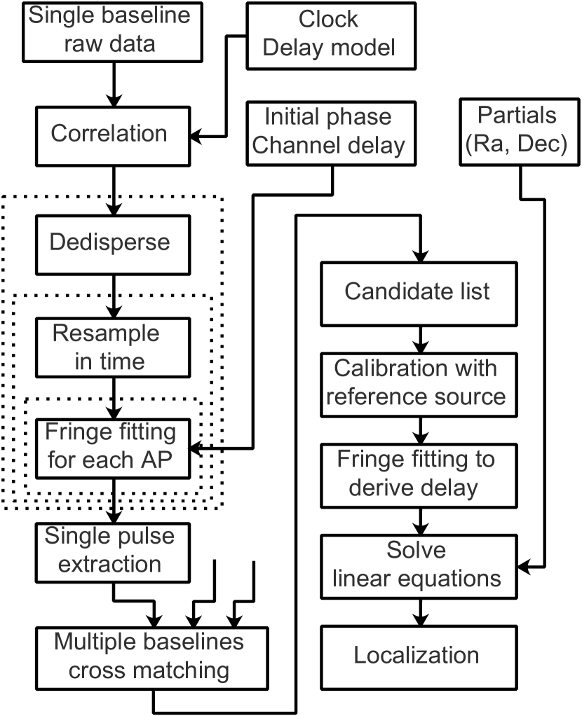
Figure 1: Demonstration of geodetic VLBI based single pulse search and localization pipeline. Steps enclosed by dotted rectangles represent iterations with corresponding quantities.

In this section, we introduce the astrometric solving method for single pulse localization. The localization part, together with the search part in Liu et al. (2018a), build up the complete pipeline for single pulse search and localization in a geodetic VLBI approach.

By assuming the burst is a point source, we are able to derive single pulse positions by solving a set of linear equations based on the relation between the residual delay and the correction to a priori position. The idea is taken directly from solutions for earth orientation parameters (EOPs, usually include precession and nutation, polar motion, universal time), baseline and source position vectors, etc. in standard geodetic and astrometric VLBI measurement (Thompson et al., 2001; Takahashi, 2000). Actually there is already work that tries to obtain the high precision pulsar position in a geodetic VLBI approach: Sekido et al. (1999) obtain the position of B0329+54 and further derive its proper motion by first deriving the group delay with Japanese bandwidth synthesis software “KOMB” (Takahashi et al., 1991), then carrying out analysis with CALC/SOLVE. However, their approach is still quite different from our work: they treat the pulsar as a normal radio source. Since B0329+54 is strong, they even do not use pulse gating. The total duration of pulsar observation that is used to derive position is as long as several hours. In contrast, in our work, we try to resolve and localize every individual single pulse with durations as short as 4 milliseconds. Actually we are the first that try to localize the single pulse in an astrometric solving approach.

Concerning this work, since the pulsar is observed in phase reference mode, most of geodetic and atmospheric effects can be removed by phase reference calibration. What we need to estimate is just the correction to a priori position for every individual single pulse. Assuming the single pulse cross spectrum has been phase reference calibrated, for each baseline, the linear relation between the residual delay and the correction to a priori position can be expressed as:

$$\tau=\frac{\partial\tau}{\partial\alpha}\Delta\alpha+\frac{\partial\tau}{\partial\delta}\Delta\delta,$$ (1)

where $\tau$ is the residual delay of this baseline, $\frac{\partial\tau}{\partial\alpha}$ and $\frac{\partial\tau}{\partial\delta}$ are partial derivatives of delay by Ra and Dec, $\Delta\alpha$ and $\Delta\delta$ are corrections to a priori position. The residual delay can be derived by fitting the fringe phase. Two partial derivatives of delay by the source position are given by VLBI delay model, and can be obtained from popular model calculation programs, e.g., CALC. The above equations are solvable with two or more baselines. The least square solutions that takes the uncertainties of residual delay into account is described in Appendix A.

Fig. 1 demonstrates the whole geodetic VLBI based single pulse search pipeline. In this pipeline, the search and localization are two independent steps. In the first step, single pulse candidates are extracted by cross spectrum fringe fitting. Cross spectrum that takes the single pulse information is extracted for further localization. In the second step, single pulse cross spectrum is calibrated with phase reference source and then fitted to derive residual delay.

The single pulse search and localization scheme described in Fig. 1 has been implemented as the “VOLKS” (VLBI Observation for single pulse Localization Keen Searcher) pipeline. At present, this pipeline supports dedispersion, fringe fitting of fast dump cross spectrum, filtering of single pulse candidates from multiple re-sampling time (window length), multiple baselines cross matching. For localization, it supports both radio imaging and astrometric solving methods. The pipeline is still being improved, so as to support more features, e.g., cross spectrum based DM search, GPU acceleration of fringe fitting, etc. We have made this pipeline publicly available (Liu, 2018, Codebase: https://github.com/liulei/volks).

3 Localization result

We carry out single pulse search and localization in a VLBI pulsar data set which has been used in Liu et al. (2018a). All works except for the AIPS calibration part are carried out with the “VOLKS” pipeline described in Sec. 2. We present the localization results using both radio imaging and astrometric solving methods and compared their accuracies.

3.1 Data set

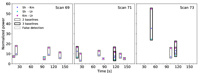
Figure 2: Single pulse detection result of VLBI pulsar data set psrf02. Single pulses detected on multiple baselines are enclosed by rectangular boxes. Thin and thick solid line rectangles correspond to those detected on 2 and 3 baselines, respectively. The only one enclosed by dotted rectangle is false detection according to its pulsar phase. Note that the actual width of the single pulse is much narrower than the width of the rectangular box. In total, 17 single pulses (including 1 false detection) are detected on 2 or 3 baselines. The detailed parameters of these single pulses together with their localization results are presented in Tab. 1.

Data is taken from CVN VLBI pulsar observation psrf02. The 96 MHz bandwidth data in S band is recorded in 6 frequency channels, 2 bits sampling. Three CVN stations, Sh, Km, Ur participate the observation. The details of the observation are presented in Liu et al. (2018a). Among the 293 scans in the 24 hours observation, single pulses of PSR J0332+5434 in Scan 69, 71 and 73 are extracted for localization. J0347+5557 in Scan 68, 70, 72 and 74 are used as phase reference source, 3C273 in Scan 293 is used for PCAL, clock and channel delay calibration.

Since CALC is easy to be integrated into the localization pipeline, in this work, we use CALC 9.1 for partial derivative, $uv$ and delay model calculation. In order to keep the consistency, we reprocess the raw data using DiFX correlator and carry out single pulse search with exactly the same procedure described in Liu et al. (2018a).

Fig. 2 presents the single pulse detection result using DiFX correlator (Deller et al., 2007, 2011). We expect it to show identical result as Fig. 5 in Liu et al. (2018a) using the CVN software correlator (Zheng et al., 2010). However, at first glance, they are not consistent with each other. According to our analysis, the main reason is, two correlators behave differently when SNR (Signal to Noise Ratio) is low. In this case, when the normalized power is less than 5, the results are different. Since two correlators use totally different delay models, it is not surprising to give such kind of discrepancy. Besides that, the implementations of the algorithm in two correlators are different. The good thing is, when it comes to strong signals, the results given by two correlator are quite consistent: singles pulses at 17.5 s of Scan 71, 49.1 s and 113.4 s of Scan 73 are detected on all 3 baselines by both correlators. However, the low sensitivity of Sh-Ur baseline still makes the result different: based on DiFX output, two singles pulses at 116.2 s and 116.9 s of Scan 71 are detected on all three baselines, while the single pulse at 21.0 s of Scan 69 is missed on Sh-Ur baseline, although it is detected on all three baselines in Liu et al. (2018a). In summary, 17 single pulses are detected on at least 2 baselines. According to their pulsar phases, we may know the one enclosed by dotted rectangle is a false detection.

We extract the visibility records that contain single pulse information from the original visibility files, and convert them together with visibilities of phase reference source (J0347+5557) and calibration source (3C273) to FITS-IDI format for further calibration and localization.

3.2 Localization

Table 1: Parameters of 17 single pulses detected in Scan 69, 71 and 73 of CVN observation psrf02. All positions are given as offsets to a priori position. The offset in Ra direction is the tangent plane projection: $\Delta\alpha^{*}=\Delta\alpha\cos\delta$. For radio imaging, we take a pixel size of 2.0 mas $\times$ 2.0 mas. SNR is calculated as the peak flux subtracted by the average flux and then normalized with noise (standard deviation).

			Baseline			Solving		Imaging
No.	Scan	Time	Km-Sh	Km-Ur	Sh-Ur	$\Delta\alpha^{*}$	$\Delta\delta$	$\Delta\alpha^{*}$	$\Delta\delta$	SNR
		(sec)				(mas)	(mas)	(mas)	(mas)
1	69	14.565	✓	✓		421.9$\pm$17.9	-313.3$\pm$15.6	392.0	-294.0	9.0
2	69	21.000	✓	✓		392.6$\pm$14.6	-223.3$\pm$13.2	358.0	-248.0	9.6
3	69	95.306		✓	✓	498.7$\pm$21.0	-203.7$\pm$25.5	468.0	-252.0	9.1
4	69	107.463	✓	✓		481.5$\pm$15.6	-264.3$\pm$13.7	460.0	-270.0	9.4
5	69	136.765	✓	✓		401.0$\pm$17.4	-263.2$\pm$16.1	392.0	-256.0	8.3
6	71	17.547	✓	✓	✓	377.9$\pm$10.2	-327.2$\pm$13.4	350.0	-306.0	11.1
7	71	26.122	✓	✓		579.7$\pm$18.1	-187.6$\pm$15.9	518.0	-222.0	8.9
8	71	75.431	✓	✓		444.9$\pm$16.0	-216.3$\pm$15.1	410.0	-192.0	8.4
9	71	86.636	✓	✓		7673.9$\pm$16.8	-2873.4$\pm$15.4	-26.0	540.0	6.5
10	71	116.158	✓	✓	✓	417.2$\pm$11.7	-225.2$\pm$13.8	396.0	-266.0	11.8
11	71	116.872	✓	✓	✓	389.6$\pm$11.7	-290.3$\pm$15.8	358.0	-288.0	10.1
12	71	131.879	✓	✓		416.5$\pm$16.4	-228.2$\pm$15.1	382.0	-234.0	9.1
13	71	142.605	✓	✓		414.4$\pm$17.5	-301.3$\pm$16.3	422.0	-290.0	8.8
14	73	49.109	✓	✓	✓	386.2$\pm$ 8.2	-280.1$\pm$ 9.4	388.0	-284.0	10.7
15	73	100.557	✓	✓		447.5$\pm$17.3	-190.4$\pm$15.5	432.0	-204.0	7.7
16	73	112.702	✓	✓		442.7$\pm$15.1	-245.5$\pm$14.6	416.0	-240.0	8.6
17	73	113.418	✓	✓	✓	433.0$\pm$10.5	-272.4$\pm$14.1	408.0	-258.0	9.5

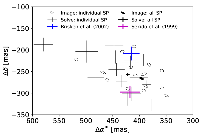
Figure 3: Localization of every individual single pulse (SP) and the average result. For comparison, two reference positions are also presented. They are calculated by evolving positions at reference epoch to the date of pulsar observation according to given proper motions. Error bars of reference positions are calculated by combing uncertainties of positions and proper motions: $\sigma=\sqrt{\sigma_{\mathrm{pos}}^{2}+(\sigma_{\mathrm{pm}}\Delta t)^{2}}$. Here $\sigma_{\mathrm{pos}}$ and $\sigma_{\mathrm{pm}}$ are uncertainties of position and proper motions in Ra and Dec directions given by references. $\Delta t$ is the time between reference epoch and date of pulsar observation. Ellipses are drawn according to the shape and position angle of the corresponding beams, which are estimated using the same algorithm as in DIFMAP (TJP’s algorithm). All positions are given as offset to a priori position. The offset in Ra direction is the tangent plane projection: $\Delta\alpha^{*}=\Delta\alpha\cos\delta$.

Table 2: Reference positions (J2000.0) and proper motions of PSR J0332+5434 at their respect reference epochs. The proper motion in Ra direction is the tangent plane projection: $\mu^{*}_{\alpha}=\mu_{\alpha}\cos\delta$.

Reference	$\alpha$	$\delta$	$\mu^{*}_{\alpha}$	$\mu_{\delta}$	Reference
			(mas/yr)	(mas/yr)	epoch
Sekido et al. (1999)	$03^{\mathrm{h}}32^{\mathrm{m}}59^{s}.3760\pm 0.0010$	$54^{\circ}34^{\prime}43^{\prime\prime}.5040\pm 0.0070$	17.30$\pm$0.80	-11.50$\pm$0.60	1995.0
Brisken et al. (2002)	$03^{\mathrm{h}}32^{\mathrm{m}}59^{s}.3862\pm 0.0017$	$54^{\circ}34^{\prime}43^{\prime\prime}.5051\pm 0.0150$	17.00$\pm$0.27	-9.48$\pm$0.37	2000.0

We use AIPS (31DEC18) for calibration. According to the standard recipe for phase reference observations, the whole process consists of 3 steps: (a) Calibrate delay and phase in every individual frequency channel (IF) for single pulses and phase reference source (J0347+5557) using the solution derived from calibration source (3C273). (b) Derive solutions for phase reference source, including delays (combining all IFs), phases and delay rates, then interpolate them to the pulsar scans. (c) Calibrate every single pulse using solutions interpolated from phase reference source and output them with FITS-IDI formats for further localization. One thing we want to point out is, the above calibration procedure is only intended for our testing pulsar data set. In real FRB search, the burst and the target source appear in the same FoV. The corresponding calibration is somewhat similar with phase reference observation, but more simplified. Please refer to Sec. 5.3 for a detailed explanation.

Our implementation of radio imaging takes similar procedure as in DIFMAP (Shepherd, 1997). The main difference is DIFMAP only deals with data that all frequency points inside one IF are summed together, which greatly reduces the time consumption of imaging process at the expense of small imaging area. However, this is based on the assumption that target source is close to its a priori position and therefore no fringe phase ambiguity exists inside one IF. For single pulse search, large ambiguities might still exist after phase calibration if the burst is far from a priori position. To keep full fringe phase ambiguity information, in this work, frequency points inside one IF are not summed together before they are gridded in the $uv$ plane.

To calculate the delay model of PSR J0332+5434 for VLBI correlation, we use a priori position (Ra: 3^h32^m59^s.368, Dec: 54^∘34^′43^′′.57, in J2000.0) given by ATNF pulsar database (Manchester et al., 2005) at reference epoch MJD 46473 (Feb. 12, 1986). The localization results are presented in Tab. 1. According to uncertainties of each single pulse given by astrometric solving, the results derived by both methods are consistent with each other in a 3$\sigma$ level. Compared with 2 baselines results, 3 baselines results usually yield smaller uncertainties and higher SNR. Among all single pulses presented here, No. 14 corresponds to the one with the highest normalized power in Fig. 2 and the smallest uncertainties. Note that its SNR is not the highest, according to our investigation, this is due to its large flux density fluctuation in image plane. Also note No. 9 in the table, which corresponds to the false detection in Fig. 2. Clearly it yields incorrect position with both radio imaging and astrometric solving methods. Moreover, positions given by two methods are inconsistent with each other.

By griding all single pulses (except for the false detection) in the $uv$ plane, we obtain the average position offset ($\Delta\alpha^{*}$: 396 mas, $\Delta\delta$: -266 mas). By solving linear equations of all single pulses (except the false detection) together, we derive the average position correction ($\Delta\alpha^{*}$: 421.7$\pm$3.3 mas, $\Delta\delta$: -257.0$\pm$3.6 mas). Mathematically, the two methods are equivalent. We expect them to give identical results. However, in the actual data processing, the imaging and fringe phase fitting procedures are totally different. For instance, the weight of each single pulse is determined by the amplitude of cross spectrum and the scatter of fringe phase, respectively. This leads to the discrepancy of the average position.

In Fig. 3, we plot the localization result of every individual single pulse and average positions given by two methods. To evaluate the absolute localization precision of the whole data processing pipeline, we also present two reference positions (Sekido et al., 1999; Brisken et al., 2002, see Tab. 2 for details). The two positions are derived by evolving the reference positions at reference epochs to pulsar observation date according to reference proper motions. As demonstrated in the figure, reference positions are roughly consistent with single pulse localization result. All single pulses except one derived by astrometric solving method distribute in a 200 mas $\times$ 200 mas area. The scatters of single pulses locations derived by radio imaging and astrometric solving methods are 53.2 mas and 65.1 mas, respectively, which can be regarded as the absolute localization precision of this work.

4 Analysis of computational cost

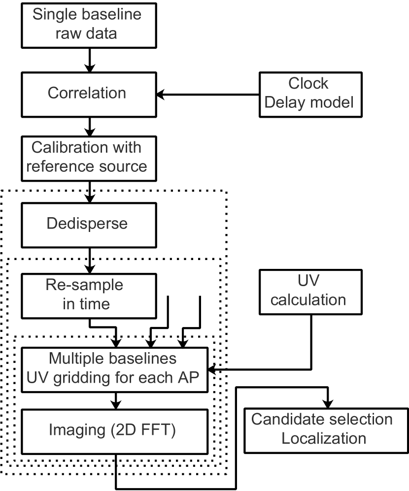
Figure 4: Demonstration of single pulse search with radio imaging pipeline. Steps enclosed by dotted rectangles represent iterations with corresponding quantities.

In this section, we analyze the computational cost of both radio imaging and geodetic VLBI based single pulse search pipeline, and come to the conclusion that the letter one is more suitable for FRB search in real observation.

Fig. 4 demonstrates the single pulse search with radio imaging pipeline. Visibilities from each baseline are first calibrated and then transformed to the image plane to create fast dumped images with multiple re-sampling times. Single pulse candidates are detected in these fast dumped images according to given threshold. To use FFT to speedup the transformation process, visibilities are gridded in the $uv$ plane (Thompson et al., 2001). In radio imaging search pipeline, the search and localization steps are coupled together: single pulses are detected and localized directly in the fast dumped images. However, such kind of scheme is only feasible for VLBI system with not very long baselines. Taking the configuration of VLA for example. The longest baseline is 36 km. In S band (2.2 GHz), the angular resolution is around 0.78 arcsec. The diameter of VLA antenna is 25 m. As a raw estimation, the corresponding FoV is 22.88 arcmin ($\sim 1.22~{}\lambda/D$). In radio imaging, the pixel size usually takes a quarter of angular resolution. To cover 80% of the FoV ($\sim\lambda/D$), the corresponding map size is 5760$\times$5760, which is reasonable for 2D FFT and the single pulse detection afterwards. However, for a typical VLBI network, e.g., Chinese VLBI Network (CVN, Zheng, 2015), the baseline is as long as 3000 km. By keeping other parameters unchanged, the corresponding map size is 480000$\times$480000, which is two orders of magnitude larger than that of VLA. Since the computational complexity of radio imaging pipeline is usually proportional to map size, the computational cost is two orders of magnitude higher. Obviously this is a huge challenge for the actual operation.

It is possible to compare the computational cost of both pipelines in an qualitative way: by investigating Fig. 1 and Fig. 4, one may find that both pipelines involve three loops. From outside to inside, they are: DM trials for dedispersion, multiple re-sampling times and series of re-sampled cross spectrum. By selecting the same re-sampling time, the two pipelines require the same number of iterations. For radio imaging, the inner most operation involves $uv$ gridding, 2D FFT and single pulse selection. The first term is negligible as it is proportional to the number of samples. In contrast, in the geodetic VLBI pipeline, the most time consuming part is fringe fitting, which involves 2D FFT to search for single band delay (SBD) and multi band delay (MBD). We may demonstrate that the size of this 2D array is much smaller than that of radio imaging. E.g., for a typical configuration of the pulsar observation in the above section, Tab. 3 present the computational complexity of both pipelines. For geodetic VLBI pipeline, according to Eq. 12 of Liu et al. (2018a), the minimum FFT size for SBD search is 1746, the number of frequency channels for MBD search is 6. By rounding them to the power of 2 and taking 4 times extrapolation, the corresponding sizes are 8192 and 32, respectively. One may find that for a baseline length of 3000 km in CVN, the actual computational cost of radio imaging is much higher than that of geodetic VLBI pipeline. It is not difficult to come to the conclusion that the geodetic VLBI pipeline is more suitable for real time FRB search than radio imaging pipeline.

Table 3: Computational complexity of two single pulse search pipelines.

Radio imaging		Geodetic VLBI
N: 480000		$N_{1}$: 8192, $N_{2}$: 32
2D FFT	$2\times\frac{34}{9}N\log_{2}(N)\times N$	2D FFT (per baseline)	$\frac{34}{9}N_{1}\log_{2}(N_{1})\times N2+\frac{34}{9}N_{2}\log_{2}(N_{2})\times N_{1}$
Finding peak	$N^{2}$	Finding peak (per baseline)	$N_{1}\times N_{2}$
Total	$\frac{68}{9}N^{2}\log_{2}(N)+N^{2}$	Total (3 baselines)	$\frac{34}{3}N_{1}N_{2}\log_{2}(N_{1}N_{2})+3N_{1}N_{2}$
	($3.31\times 10^{13}$)		($5.43\times 10^{7}$)

5 Discussion

5.1 Subtraction of constant sources

Single pulse search is usually carried out as commensal task in regular VLBI observations. In this case, how to remove the influence of target source and other constant sources is a problem that must be solved. The “realfast” pipeline deals with this problem by subtracting the mean visibility in time on timescales less than the VLA fringe rate. Similar treatment is suitable for our geodetic VLBI based pipeline, too. Besides that, we propose another scheme which is specially designed for fringe fitting pipeline: to carry out single pulse search, the clock is well adjusted (fringe rate less than $10^{-3}$ Hz), the MBD and SBD for the target source does not change too much in the whole scan. We may skip the target source and the surrounding area in the MBD and SBD search matrix. However, this scheme can only be verified with data in which fast transients present together with constant source, which is not available at present. In this case, mean visibilities subtraction scheme might be more reasonable.

5.2 Large search area

One might doubt that if it is possible to detect single pulses efficiently in the whole FoV with our method. In Liu et al. (2018a), we point out that the fringe fitting process is somewhat similar with that of coherent beam forming, but without the computational expense to form a great number of beams to cover the whole FoV of telescopes. For localization, traditionally, we only carry out narrow field imaging. The corresponding searching area is much smaller than the FoV. The main reason is, the delay model is (usually) calculated for the center of FoV but applied to the whole FoV. The residual delay rate is large at the edge of the FoV. The signal degrades quickly as the integration becomes long. In regular VLBI correlation, the integration time is as long as 1 second. In contrast, in our single pulse detection method, the maximum integration time is no more than 32 ms, and is usually as short as 4 ms. This short integration time makes it possible to investigate the whole FoV with only one image. Actually this is somewhat similar with the implementation of multiple phase center in modern VLBI correlator (Deller et al., 2011; Keimpema et al., 2015). For instance, in SFXC, for each sub-integration period (25 ms), a phase shift is performed for each phase center, so as to compensate for the phase change due to the large residual delay rate in that position. We know that although the signal will not degrade very much within such a short time, the corresponding SNR is low. In this work, we have demonstrated that it is still possible to detect signals for such a short integration time.

For the localization of single pulse in the whole FoV, one of the drawbacks of radio imaging is the computational cost increases significantly when the imaging area becomes large in long baseline observation. In contrast, in the geodetic VLBI search scheme, this is not a problem. We have to admit that when the single pulse is far from phase center, e.g., close to $\frac{1}{2}~{}\theta_{\mathrm{FWHM}}$, the performance of the search pipeline is still not clear. Possible problems include the decrease of detection sensitivity, the increase of localization uncertainty, etc. Although these problems also exist in the radio imaging based search scheme, we have not seen their related descriptions and solutions. Therefore, we propose to carry out further VLBI observation to test the pipeline. For instance, by placing the pulsar in the FoV with different offsets to the phase center, such that we may plot the power and localization precision of the detected single pulses as a function of offset to FoV center.

5.3 Localization in geodetic VLBI observation

The VLBI observation that provides the pulsar data set used in this work is carried out in phase reference mode, which makes it possible to calibrate the extracted single pulses with phase reference source. However, geodetic VLBI obervation takes a totally different approach: to cover as large sky area as possible, sources distribute evenly in the sky. In this case, it is still possible to localize the burst: the target source itself is a perfect phase reference source. Since the burst and the target source always appear in the same FoV, it is even not necessary to extrapolate the fringe fitting solution to the burst time. We may just derive MBD, SBD, delay rate and residual phase for the target source in the scan, and then calibrate the visibilities with these quantities. Single pulse search is carried out with calibrated visibilities. Once single pulse is detected, the derived delay can be used directly for localization with astrometric method. No further calibration with phase reference source is needed.

5.4 Dispersion measure search

One thing we want to point out is we do not carry out dispersion measure search in this work. The DM value provided by ATNF pulsar database is used for dedispersion. The main reason is the DM value of PSR J0332+5434 is too low (26.833 $\mathrm{pc~{}cm}^{-3}$). In Liu et al. (2018a), we have proposed a DM search scheme, which is quite straight forward: dividing the DM search range into multiple bins, then carrying out dedispersion and single pulses search independently for these bins. For a minimum re-sampling time of 4.096 ms and a frequency range of 2192 MHz to 2288 MHz, the corresponding DM resolution is 57.7 $\mathrm{pc~{}cm}^{-3}$, which is too large to resolve the DM of this pulsar. Since DM search is an important part in the whole single pulse search pipeline, we propose to observe RRAT (McLaughlin et al., 2007) sources to obtain high DM data to test our geodetic VLBI based search pipeline. Our observation proposal has been submitted to EVN, and is scheduled in March, 2019.

6 Conclusions

In this paper, we present the astrometric solving based single pulse localization method. By applying this method to a VLBI pulsar observation data set, we demonstrate that the localization result for each single pulse derived by both radio imaging and astrometric solving are consistent with each other in a 3 $\sigma$ level. Most of single pulses, together with reference positions, distribute in a 200 mas $\times$ 200 mas area. The scatters of localization results using both methods are less than 70 mas, which can be regarded as the absolute localization precision. Our work proves that it is possible to derive single pulse position with reasonable precision based on just 3 or even 2 baselines and 4 ms integration in VLBI observation. The localization method, together with the single pulse search method in Liu et al. (2018a), build up the complete geodetic VLBI based single pulse search and localization pipeline. We further demonstrate that the computational cost of radio imaging pipeline is much higher than that of geodetic VLBI based pipeline. Therefore, for cross spectrum based FRB search in VLBI observation, geodetic VLBI pipeline might be a better choice. We name our pipeline as “VOLKS” and have made it publicly available. We hope this will be helpful for radio transient studies.

Appendix A Least square solutions

The derive of offset ($\Delta\alpha,\Delta\delta$) to a priori position is divided into two steps.

(a) Fitting residual delay. For every single pulse, the delay $\tau$ for each baseline is derived by fitting the fringe phase $\phi_{k}$ after phase reference calibration as a function of frequency $f_{k}$:

$$\phi_{k}=2\pi f_{k}\tau+\phi_{0}.$$ (A1)

The fit of above linear equation by using the amplitude of each frequency point $f_{k}$ as weight is available in most mathematical libraries. After fitting, we obtain the delay $\tau_{i}$ and the corresponding uncertainties $\sigma_{i}$ for baseline $i$. The relation between $\sigma_{i}$ and the scatter of fringe phase is explained in Takahashi (2000). Note that when the source is far from a priori position, fringe phase ambiguity exists even after calibration. In this case we have to compensate an initial delay value to remove ambiguity before fitting.

(b) Derive position offset. This is to solve the linear equation:

$$\mathbf{y}=\mathbf{A}\mathbf{x}.$$ (A2)

Here $\mathbf{y}=(\tau_{1},\tau_{2},...,\tau_{n})^{T}$ is the delay vector for $n$ baselines. $\mathbf{x}=(\Delta\alpha,\Delta\delta)^{T}$ is the position offset vector. $\mathbf{A}=(A_{1},A_{2},...,A_{n})^{T}$ is the partial derivative matrix: $A_{i}=\left(\frac{\partial\tau_{i}}{\partial\alpha},\frac{\partial\tau_{i}}{\partial\delta}\right)$. The least square solution of above equations is:

$$\mathbf{\hat{x}}=(\mathbf{A}^{T}\mathbf{WA})^{-1}\mathbf{A}^{T}\mathbf{Wy}.$$ (A3)

Here $\mathbf{W}$ is the weight matrix: $\mathbf{W}=\mathbf{\Sigma}^{-1}$. $\mathbf{\Sigma}=\mathrm{diag}(\sigma_{1}^{2},\sigma_{2}^{2},...,\sigma_{n}^{2})$ is the delay error matrix. The estimation parameter error matrix is:

$$\mathbf{\Sigma_{p}}=(\mathbf{A}^{T}\mathbf{\Sigma}^{-1}\mathbf{A})^{-1}.$$ (A4)

The square root of $\Sigma_{\mathrm{p},11}$ and $\Sigma_{\mathrm{p},22}$ correspond to uncertainties of $\Delta\alpha$ and $\Delta\delta$, respectively.

References

- (1)
- Amiri et al. (2018) The CHIME/FRB Collaboration, Amiri, M., Bandura, K., et al. 2018, ApJ, 863, 48
- The CHIME/FRB Collaboration et al. (2019a) The CHIME/FRB Collaboration, Amiri, M., et al. 2019a, Nature, 566, 230
- The CHIME/FRB Collaboration et al. (2019b) The CHIME/FRB Collaboration, Amiri, M., et al. 2019b, Nature, 566, 235
- Bassa et al. (2017) Bassa, C. G., Tendulkar, S. P., Adams, E. A. K., et al. 2017, ApJ, 843, L8
- Bhandari et al. (2018) Bhandari, S., Keane, E. F., Barr, E. D., et al. 2018, MNRAS, 475, 1427
- Brisken et al. (2002) Brisken, W. F., Benson, J. M., Goss, W. M., & Thorsett, S. E. 2002, ApJ, 571, 906
- Caleb et al. (2016) Caleb, M., Flynn, C., Bailes, M., et al. 2016, MNRAS, 458, 718
- Caleb et al. (2017) Caleb, M., Flynn, C., Bailes, M., et al. 2017, MNRAS, 468, 3746
- Champion et al. (2016) Champion, D. J., Petroff, E., Kramer, M., et al. 2016, MNRAS, 460, L30
- Chatterjee et al. (2017) Chatterjee, S., Law, C. J., Wharton, R. S., et al. 2017, Nature, 541, 58
- Deller et al. (2011) Deller, A. T., Brisken, W. F., Phillips, C. J., et al. 2011, PASP, 123, 275
- Deller et al. (2007) Deller, A. T., Tingay, S. J., Bailes, M., & West, C. 2007, PASP, 119, 318
- Farah et al. (2018) Farah, W., Flynn, C., Bailes, M., et al. 2018, MNRAS, 478, 1209
- Fialkov et al. (2018) Fialkov, A., Loeb, A., & Lorimer, D. R. 2018, ApJ, 863, 132
- Johnston et al. (2008) Johnston, S., Taylor, R., Bailes, M., et al. 2008, Experimental Astronomy, 22, 151
- Katz (2016) Katz, J. I. 2016a, Modern Physics Letters A, 31, 1630013
- Keane & Petroff (2015) Keane, E. F., & Petroff, E. 2015, MNRAS, 447, 2852
- Keimpema et al. (2015) Keimpema, A., Kettenis, M. M., Pogrebenko, S. V., et al. 2015, Experimental Astronomy, 39, 259
- Law & Bower (2012) Law, C. J., & Bower, G. C. 2012, ApJ, 749, 143
- Law et al. (2015) Law, C. J., Bower, G. C., Burke-Spolaor, S., et al. 2015, ApJ, 807, 16
- Law et al. (2011) Law, C. J., Jones, G., Backer, D. C., et al. 2011, ApJ, 742, 12
- Liu et al. (2018a) Liu, L., Tong, F., Zheng, W., Zhang, J., & Tong, L. 2018a, AJ, 155, 98
- Liu et al. (2018b) Liu, L., Zheng, W., Yan, Z., & Zhang, J. 2018b, Research in Astronomy and Astrophysics, 18, 069
- Liu (2018) Liu, L. 2018, VOLKS: VLBI Observation for frb Localization Keen Searcher, v0.7-alpha, Zenodo, doi:10.5281/zenodo.2565124
- Lorimer et al. (2007) Lorimer, D. R., Bailes, M., McLaughlin, M. A., Narkevic, D. J., & Crawford, F. 2007, Science, 318, 777
- Macquart et al. (2018) Macquart, J.-P., Shannon, R. M., Bannister, K. W., et al. 2018, arXiv:1810.04353, submitted to ApJL
- Manchester et al. (2005) Manchester, R. N., Hobbs, G. B., Teoh, A., & Hobbs, M. 2005, AJ, 129, 1993
- Marcote et al. (2017) Marcote, B., Paragi, Z., Hessels, J. W. T., et al. 2017, ApJ, 834, L8
- McLaughlin et al. (2007) McLaughlin, M. A., Rea, N., Gaensler, B. M., et al. 2007, ApJ, 670, 1307
- Ng et al. (2017) Ng, C., Vanderlinde, K., Paradise, A., et al. 2017, arXiv:1702.04728, submitted to the XXXII International Union of Radio Science General Assembly & Scientific Symposium (URSI GASS) 2017
- Paragi (2016) Paragi, Z. 2016, arXiv:1612.00508, submitted to the proceedings of the 13th EVN Symposium and Users Meeting
- Petrachenko et al. (2013) Petrachenko, W., Behrend, D., Hase, H., et al. 2013, EGUGA, 15
- Petroff et al. (2016) Petroff, E., Barr, E. D., Jameson, A., et al. 2016, PASA, 33, e045
- Petroff et al. (2017) Petroff, E., Burke-Spolaor, S., Keane, E. F., et al. 2017, MNRAS, 469, 4465
- Ravi et al. (2015) Ravi, V., Shannon, R. M., & Jameson, A. 2015, ApJ, 799, L5
- Scholz et al. (2017) Scholz, P., Bogdanov, S., Hessels, J. W. T., et al. 2017, ApJ, 846, 80
- Sekido et al. (1999) Sekido, M., Imae, M., Hanado, Y., et al. 1999, PASJ, 51, 595
- Shannon et al. (2018) Shannon, R. M., Macquart, J.-P., Bannister, K. W., et al. 2018, Nature, 562, 386
- Shepherd (1997) Shepherd, M. C. 1997, Astronomical Data Analysis Software and Systems VI, 125, 77
- Spitler et al. (2016) Spitler, L. G., Scholz, P., Hessels, J. W. T., et al. 2016, Nature, 531, 202
- Takahashi (2000) Takahashi, H., et al., 2000, “Wave Summit Course: Very Long Baseline Interferometer.” Ohmsha. Ltd.
- Takahashi et al. (1991) Takahashi, Y., Hama, S., Kond, T. 1991, J. Communication Research Lab. 38, 481
- Tendulkar et al. (2017) Tendulkar, S. P., Bassa, C. G., Cordes, J. M., et al. 2017, ApJ, 834, L7
- Thompson et al. (2001) Thompson, A. R., Moran, J. M., & Swenson, G. W., Jr. 2001, “Interferometry and synthesis in radio astronomy by A. Richard Thompson, James M. Moran, and George W. Swenson, Jr. 2nd ed. New York : Wiley, c2001.xxiii, 692 p. : ill. ; 25 cm. ”A Wiley-Interscience publication.“ Includes bibliographical references and indexes. ISBN : 0471254924”
- Thompson et al. (2011) Thompson, D. R., Wagstaff, K. L., Brisken, W. F., et al. 2011, ApJ, 735, 98
- Thornton et al. (2013) Thornton, D., Stappers, B., Bailes, M., et al. 2013, Science, 341, 53
- Wayth et al. (2011) Wayth, R. B., Brisken, W. F., Deller, A. T., et al. 2011, ApJ, 735, 97
- Zheng (2015) Zheng, W. 2015, IAUGA, 22, 2255896
- Zheng et al. (2010) Zheng, W., Quan, Y., Shu, F., et al. 2010ivsg_conf, 157