Multiple Scaled Contaminated Normal Distribution
and Its Application in Clustering

Abstract

The multivariate contaminated normal (MCN) distribution represents a simple heavy-tailed generalization of the multivariate normal (MN) distribution to model elliptical contoured scatters in the presence of mild outliers, referred to as "bad" points. The MCN can also automatically detect bad points. The price of these advantages is two additional parameters, both with specific and useful interpretations: proportion of good observations and degree of contamination. However, points may be bad in some dimensions but good in others. The use of an overall proportion of good observations and of an overall degree of contamination is limiting. To overcome this limitation, we propose a multiple scaled contaminated normal (MSCN) distribution with a proportion of good observations and a degree of contamination for each dimension. Once the model is fitted, each observation has a posterior probability of being good with respect to each dimension. Thanks to this probability, we have a method for simultaneous directional robust estimation of the parameters of the MN distribution based on down-weighting and for the automatic directional detection of bad points by means of maximum a posteriori probabilities. The term "directional" is added to specify that the method works separately for each dimension. Mixtures of MSCN distributions are also proposed as an application of the proposed model for robust clustering. An extension of the EM algorithm is used for parameter estimation based on the maximum likelihood approach. Real and simulated data are used to show the usefulness of our mixture with respect to well-established mixtures of symmetric distributions with heavy tails.

Keywords: contaminated normal distribution, heavy-tailed distributions, multiple-scaled distributions, EM algorithm, mixture models, model-based clustering.

1 Introduction

Statistical inference dealing with continuous multivariate data is commonly focused on the multivariate normal (MN) distribution, with mean $\boldsymbol{\mu}$ and covariance matrix $\boldsymbol{\Sigma}$, due to its computational and theoretical convenience. However, for many applied problems, the tails of this distribution are lighter than required. This is often due to the presence of outliers, i.e., observations that do not comply with the model assumed and that affect the estimation of $\boldsymbol{\mu}$ and $\boldsymbol{\Sigma}$ (Maronna and Yohai, 2014). This has created a need for techniques that detect outliers and for which parameter estimates are robust in their presence (see, e.g., Devlin et al., 1981 and Rousseeuw and Leroy, 2005).

Outliers may roughly be divided into two types: mild and gross (Ritter, 2015). Outliers are "mild" with respect to the MN distribution (reference distribution) when they do not deviate from the assumed MN model and are not strongly outlying; rather, they produce an overall distribution that is too heavy-tailed to be modeled by the MN. For a discussion of the concept of reference distribution, see Davies and Gather (1993). Therefore, mild outliers (also referred to as bad points herein, in analogy with Aitkin and Wilson, 1980) can be modeled by means of more-flexible distributions, usually symmetric and endowed with heavy tails (Ritter, 2015). To define them, the MN distribution is typically embedded in a larger symmetric model with one or more additional parameters denoting the deviation from normality in terms of tail weight. In this context, the multivariate $t$ (M$t$) distribution (see, e.g., Lange et al., 1989 and Kotz and Nadarajah, 2004), the heavy-tailed versions of the multivariate power exponential (MPE) distribution (Gómez-Villegas et al., 2011), and the multivariate leptokurtic-normal (MLN) distribution (Bagnato et al., 2017), represent possible symmetric alternatives in the subclass of the elliptically contoured distributions.

Although the methods discussed above robustify the estimation of $\boldsymbol{\mu}$ and $\boldsymbol{\Sigma}$ of the reference MN distribution, they do not allow for the automatic detection of bad points. To overcome this problem, we can consider the multivariate contaminated normal (MCN) distribution of Tukey (1960), a further common and simple elliptically contoured generalization of the MN distribution having heavier tails for the occurrence of bad points; it is a two-component normal mixture in which one of the components, with a large prior probability $\alpha$, represents the good observations (reference distribution), and the other, with a small prior probability $1-\alpha$, the same mean $\boldsymbol{\mu}$, and an inflated (with respect to $\eta>1$) covariance matrix $\eta\boldsymbol{\Sigma}$, represents the bad observations (Aitkin and Wilson, 1980). Advantageously, once the MCN distribution is fitted to the observed data by means of maximum a posteriori probabilities, each observation, if desired (Berkane and Bentler, 1988), can be classified as good or bad. Moreover, bad points are automatically down-weighted in the estimation of $\boldsymbol{\mu}$ and $\boldsymbol{\Sigma}$. Thus, the MCN distribution represents a model for the simultaneous robust estimation of $\boldsymbol{\mu}$ and $\boldsymbol{\Sigma}$ and the detection of mild outliers.

However, the MCN distribution has some drawbacks that are listed below.

1. When the scale matrix $\boldsymbol{\Sigma}$ of the MCN distribution is diagonal, the variates are pairwise uncorrelated but can be statistically dependent (with strength of dependence depending on the values of the parameters $\alpha$ and $\eta$).

2. In relation to the previous point, the product of independent univariate CN distributions, with the same parameters $\alpha$ and $\eta$, is not an MCN distribution.

3. The MCN distribution, being a normal-scale mixture, belongs to the subclass of elliptically contoured distributions (see, e.g., Gómez et al., 2003, p. 347). Thus, its flexibility in terms of shapes is limited.

4. Another limitation of the MCN distribution is that all marginals are CN distributions with the same parameters $\alpha$ and $\eta$ and, hence, the same amount of tail weight. Therefore, it is not possible to account for very different tail behaviors across dimensions.

5. In terms of robustness, bad points are automatically down-weighted in the maximum likelihood (ML) estimation of $\boldsymbol{\mu}$ and $\boldsymbol{\Sigma}$ but in the same way for each dimension. This does not take into consideration the fact that points may be bad in some dimensions but good in others, a setting that is known in the literature as dimension-wise contamination (Alqallaf et al., 2009). Thus, the down-weighting should be allowed to vary over dimensions.

6. In relation to the previous point, the procedure to detect outliers induced by the MCN distribution could be defined as omnibus in the sense that when a point is detected as bad, it is globally bad. As a practical consequence, once the point is detected as bad, we do not know the dimension(s) yielding this decision.

To overcome these drawbacks, we introduce the multiple scaled contaminated normal (MSCN) distribution. The genesis of our model follows the idea developed by Forbes and Wraith (2014) to define the multiple scaled $t$ (MS$t$) distribution. The key elements of the approach are the introduction of a multidimensional Bernoulli variable (indicating whether a point is good or bad separately for each dimension) and the decomposition of $\boldsymbol{\Sigma}$ by eigenvalues and eigenvectors matrices $\boldsymbol{\Lambda}$ and $\boldsymbol{\Gamma}$. The result is a distribution in which the scalar parameters $\alpha$ and $\eta$ of the MCN distribution are replaced by two vectors, $\boldsymbol{\alpha}$ and $\boldsymbol{\eta}$, controlling the proportion of good points and the degree of contamination, respectively, separately for each dimension induced by $\boldsymbol{\Gamma}$.

The MSCN distribution offers a remedy to the drawbacks of the MCN distribution discussed above in the following way. With respect to drawback (a), if the scale matrix $\boldsymbol{\Sigma}$ of the MSCN distribution is diagonal, then the variates are independent; as a by-product of this property, the MSCN distribution contains the product of independent univariate CN distributions as a special case, thus providing a remedy to drawback (b). With respect to drawback (c), our distribution allows for a greater variety of shapes and, in particular, contours that are symmetric but not necessarily elliptical. As concerns drawback (d), the MSCN distribution allows for the parameters $\alpha$ and $\eta$ to be set or estimated differently in each dimension. It is then possible to account for very different tail behaviors across dimensions. With respect to drawback (e), the down-weighting of the observations, in the estimation of $\boldsymbol{\mu}$ and $\boldsymbol{\Lambda}$, is allowed to vary over dimensions (directional robustness). Finally, with respect to drawback (f), the procedure to detect outliers induced by the MSCN distribution works separately for each dimension, such that a point may be detected as bad with respect to some dimensions only (directional outlier detection).

The paper is organized as follows. Section 2, after the recapitulation of some results surrounding the MCN distribution, presents the main contribution of the work (namely, the MSCN distribution and its genesis). Section 3 illustrates the use of the MSCN distribution in robust clustering based on mixture models, which is a further proposal of the present paper. This section also presents a variant of the EM algorithm to fit mixtures of MSCN distributions. Further computational and operational aspects are discussed in Section 4. Section 5 investigates the performance of the proposed mixture, in comparison with mixtures of some well-established multivariate symmetric distributions with heavy tails, with regard to artificial and real data. Conclusions, as well as avenues for further research, are given in Section 6.

2 Methodology

2.1 Preliminaries: The Multivariate Contaminated Normal

A $d$-variate random vector $\boldsymbol{X}=\left(X_{1},\ldots,X_{d}\right)^{\top}$ is said to follow the multivariate contaminated normal (MCN) distribution with mean vector $\boldsymbol{\mu}$, scale matrix $\boldsymbol{\Sigma}$, proportion of good points $\alpha\in\left(0,1\right)$, and degree of contamination $\eta>1$ if its joint probability density function (pdf) is given by

$$f_{\text{MCN}}\left(\boldsymbol{x};\boldsymbol{\mu},\boldsymbol{\Sigma},\alpha,\eta\right)=\alpha f_{\text{MN}}\left(\boldsymbol{x};\boldsymbol{\mu},\boldsymbol{\Sigma}\right)+\left(1-\alpha\right)f_{\text{MN}}\left(\boldsymbol{x};\boldsymbol{\mu},\eta\boldsymbol{\Sigma}\right),$$ (1)

where $f_{\text{MN}}\left(\cdot;\boldsymbol{\mu},\boldsymbol{\Sigma}\right)$ denotes the pdf of a $d$-variate random vector having the multivariate normal (MN) distribution with mean vector $\boldsymbol{\mu}$ and covariance matrix $\boldsymbol{\Sigma}$. In the following, when $d=1$, we will substitute the subscripts MN and MCN with N and CN, respectively. If $\boldsymbol{X}$ follows the MCN distribution, we write $\boldsymbol{X}\sim\mathcal{CN}_{d}\left(\boldsymbol{\mu},\boldsymbol{\Sigma},\alpha,\eta\right)$. As a special case of (1), if $\alpha$ and $\eta$ tend to one, we obtain the MN distribution with mean vector $\boldsymbol{\mu}$ and covariance matrix $\boldsymbol{\Sigma}$; in symbols, $\boldsymbol{X}\sim\mathcal{N}_{d}\left(\boldsymbol{\mu},\boldsymbol{\Sigma}\right)$.

An advantage of (1) with respect to the multivariate $t$ (M$t$) distribution is that, once the parameters in $\boldsymbol{\vartheta}=\{\boldsymbol{\mu},\boldsymbol{\Sigma},\alpha,\eta\}$ are estimated (for example, $\widehat{\boldsymbol{\vartheta}}=\{\widehat{\boldsymbol{\mu}},\widehat{\boldsymbol{\Sigma}},\widehat{\alpha},\widehat{\eta}\}$), we can establish whether a generic point $\boldsymbol{x}^{*}$ is good via the a posteriori probability

$$P\left(\text{$\boldsymbol{x}^{*}$ is good}\left|\widehat{\boldsymbol{\vartheta}}\right.\right)=\widehat{\alpha}f_{\text{MN}}\left(\boldsymbol{x}^{*};\widehat{\boldsymbol{\mu}},\widehat{\boldsymbol{\Sigma}}\right)\Big{/}f_{\text{MCN}}\left(\boldsymbol{x}^{*};\widehat{\boldsymbol{\vartheta}}\right),$$ (2)

and $\boldsymbol{x}^{*}$ will be considered good if $P(\text{$\boldsymbol{x}^{*}$ is good}|\widehat{\boldsymbol{\vartheta}})>1/2$, while it will be considered bad otherwise.

2.2 Proposal: Multiple Scaled Contaminated Normal

In the same spirit of Forbes and Wraith (2014), we propose the extension of the MCN distribution to a multiple scaled CN (MSCN) distribution. It consists in using the classical eigen decomposition $\boldsymbol{\Sigma}=\boldsymbol{\Gamma}\boldsymbol{\Lambda}\boldsymbol{\Gamma}^{\top}$ of the scale matrix, where $\boldsymbol{\Lambda}$ is the diagonal matrix of the eigenvalues of $\boldsymbol{\Sigma}$ and $\boldsymbol{\Gamma}$ is a $d\times d$ orthogonal matrix whose columns are the normalized eigenvectors of $\boldsymbol{\Sigma}$, ordered according to their eigenvalues. Each element in the right-hand side of this decomposition has a different geometric interpretation: $\boldsymbol{\Lambda}$ determines the size and shape of the scatter, while $\boldsymbol{\Gamma}$ determines its orientation. Moreover, we introduce the indicator variable $V_{h}$ to be good ($V_{h}=1$) or bad ($V_{h}=0$) with respect to the $h$th dimension, $h=1,\ldots,d$, and further define the $d\times d$ diagonal matrix of inverse weights as:

$$\boldsymbol{W}_{\boldsymbol{v}}=\text{diag}\left\{\left(v_{1}+\frac{1-v_{1}}{\eta_{1}}\right)^{-1},\ldots,\left(v_{d}+\frac{1-v_{d}}{\eta_{d}}\right)^{-1}\right\},$$

where $\boldsymbol{v}=\left(v_{1},\ldots,v_{d}\right)^{\top}$.

Based on the quantities introduced above, our MSCN distribution can be written as:

$$f_{\text{MSCN}}\left(\boldsymbol{x};\boldsymbol{\mu},\boldsymbol{\Gamma},\boldsymbol{\Lambda},\boldsymbol{\alpha},\boldsymbol{\eta}\right)=\sum_{h=1}^{d}\sum_{v_{h}=0}^{1}f_{\text{MN}}\left(\boldsymbol{x};\boldsymbol{\mu},\boldsymbol{\Gamma}\boldsymbol{W}_{\boldsymbol{v}}\boldsymbol{\Lambda}\boldsymbol{\Gamma}^{\top}\right)p_{v_{h}}\left(v_{h};\alpha_{h}\right),$$ (3)

where $\boldsymbol{\alpha}=\left(\alpha_{1},\ldots,\alpha_{d}\right)^{\top}$, $\boldsymbol{\eta}=\left(\eta_{1},\ldots,\eta_{d}\right)^{\top}$, and

$$p_{\boldsymbol{v}}\left(v_{1},\ldots,v_{d};\boldsymbol{\alpha}\right)=\prod_{h=1}^{d}p_{v_{h}}\left(v_{h};\alpha_{h}\right),$$

with $p_{v_{h}}\left(v_{h};\alpha_{h}\right)=\alpha_{h}^{v_{h}}\left(1-\alpha_{h}\right)^{1-v_{h}}$. If $\boldsymbol{X}$ follows the MSCN distribution, we write $\boldsymbol{X}\sim\mathcal{SCN}_{d}\left(\boldsymbol{\mu},\boldsymbol{\Gamma},\boldsymbol{\Lambda},\boldsymbol{\alpha},\boldsymbol{\eta}\right)$. The pdf in (3) can be equivalently written as:

$$f_{\text{MSCN}} \left(\boldsymbol{x};\boldsymbol{\mu},\boldsymbol{\Gamma},\boldsymbol{\Lambda},\boldsymbol{\alpha},\boldsymbol{\eta}\right)=\prod_{h=1}^{d}\left[\alpha_{h}f_{\text{N}}\left(\left[\boldsymbol{\Gamma}^{\top}\left(\boldsymbol{x}-\boldsymbol{\mu}\right)\right]_{h};0,\lambda_{h}\right)\right]^{v_{h}}$$

$$\qquad\times\left[\left(1-\alpha_{h}\right)f_{\text{N}}\left(\left[\boldsymbol{\Gamma}^{\top}\left(\boldsymbol{x}-\boldsymbol{\mu}\right)\right]_{h};0,\eta_{h}\lambda_{h}\right)\right]^{\left(1-v_{h}\right)},$$ (4)

where $\left[\boldsymbol{\Gamma}^{\top}\left(\boldsymbol{x}-\boldsymbol{\mu}\right)\right]_{h}$ denotes the $h$th element of the $d$-dimensional vector $\boldsymbol{\Gamma}^{\top}\left(\boldsymbol{x}-\boldsymbol{\mu}\right)$ and $\lambda_{h}$ the $h$th diagonal element of $\boldsymbol{\Lambda}$ (or, equivalently, the $h$th eigenvalue of $\boldsymbol{\Sigma}$).

In the bivariate case ($d=2$), Figure 1 shows, via isodensities, some possible shapes of the MSCN distribution by varying $\boldsymbol{\Gamma}$, $\boldsymbol{\alpha}$, and $\boldsymbol{\eta}$, with the mean vector and the eigenvalue matrix fixed, respectively, to $\boldsymbol{\mu}=\boldsymbol{0}$ and $\boldsymbol{\Lambda}=0.75\boldsymbol{I}$, where $\boldsymbol{I}$ denotes the identity matrix.

(a) $\theta=0$, $\boldsymbol{\alpha}=\left(0.7,0.6\right)^{\top}$ and $\boldsymbol{\eta}=\left(3,2\right)^{\top}$

(b) $\theta=\pi/6$, $\boldsymbol{\alpha}=\left(0.7,0.6\right)^{\top}$ and $\boldsymbol{\eta}=\left(3,2\right)^{\top}$

(c) $\theta=\pi/6$, $\boldsymbol{\alpha}=\left(0.7,0.7\right)^{\top}$ and $\boldsymbol{\eta}=\left(10,10\right)^{\top}$

(d) $\theta=\pi/6$, $\boldsymbol{\alpha}=\left(0.95,0.95\right)^{\top}$ and $\boldsymbol{\eta}=\left(10,10\right)^{\top}$

Figure 1: Examples of contour plots of bivariate SCN distributions with $\boldsymbol{\mu}=\boldsymbol{0}$ and $\boldsymbol{\Lambda}=0.75\boldsymbol{I}$.

The orientation matrix $\boldsymbol{\Gamma}$ is seen as a rotation matrix of angle $\theta$, that is

$$\boldsymbol{\Gamma}\left(\theta\right)=\begin{pmatrix}\cos\theta&-\sin\theta\\[4.30554pt] \sin\theta&\cos\theta\end{pmatrix}.$$

Figure 1 clearly shows how the shape of the MSCN distribution is not constrained as elliptical, although the symmetry is preserved. In particular, the choices made for $\boldsymbol{\alpha}$ and $\boldsymbol{\eta}$ produce, among others, "smoothed" rhomboidal (Figure 1(a) and 1(b)) and starred (Figure 1(c) and 1(d)) contours.

Finally, it is easy to show that if $\boldsymbol{Y}\sim\mathcal{N}_{d}\left(\boldsymbol{0},\boldsymbol{I}\right)$, then:

$$\boldsymbol{X}=\boldsymbol{\mu}+\boldsymbol{\Gamma}\boldsymbol{\Lambda}^{\frac{1}{2}}\boldsymbol{W}_{\boldsymbol{v}}^{\frac{1}{2}}\boldsymbol{Y}\sim\mathcal{SCN}_{d}\left(\boldsymbol{\mu},\boldsymbol{\Gamma},\boldsymbol{\Lambda},\boldsymbol{\alpha},\boldsymbol{\eta}\right).$$ (5)

This alternative way to see the MSCN distribution may be useful for random generation. Moreover, Equation (5) makes it easier to see that univariate marginal distributions are linear combinations of CN distributions with the same mean $\mu_{h}$, $h=1,\ldots,d$, for which, in general, no closed-form expression is available, although it is possible to show that symmetry is preserved. Therefore, univariate marginal distributions are not in general CN distributions.

3 The Mixtures of MSCN Distributions

Finite mixtures of distributions are commonly used in statistical modeling as a powerful device for clustering and classification by often assuming that each mixture component represents a cluster (or group) into the original data (see McLachlan and Basford, 1988, Fraley and Raftery, 1998, Böhning, 2000 and McNicholas, 2016).

For continuous multivariate random variables, attention is commonly focused on mixtures of MN distributions. However, in clustering applications, data are often contaminated by mild outliers (see, e.g., Bock, 2002, Gallegos and Ritter, 2009, and Ritter, 2015), affecting the estimation of the component means and covariance matrices and the recovery of the underlying clustering structure. For MN mixtures (MNMs), one of the possible solutions used to deal with mild outliers is the "component-wise" approach: the component MN distributions are separately protected against mild outliers by embedding them in more general heavy-tailed, usually symmetric, multivariate distributions. Examples are M$t$ mixtures (M$t$Ms; McLachlan and Peel, 1998 and Peel and McLachlan, 2000), MPE mixtures (MPEMs; Zhang and Liang, 2010 and Dang et al., 2015), MLN mixtures (Bagnato et al., 2017), and MS$t$ mixtures (Forbes and Wraith, 2014). These methods robustify the estimation of the component means and covariance matrices with respect to mixtures of MN distributions, but they do not allow for automatic detection of bad points, although an a posteriori procedure (i.e., a procedure taking place once the model is fitted) to detect bad points with MS$t$Ms is illustrated by McLachlan and Peel (2000). To overcome this problem, Punzo and McNicholas (2016) introduced MCN mixtures (MCNMs); for further recent uses of the MCN distribution in model-based clustering, see Punzo and McNicholas (2014, 2017), Punzo and Maruotti (2016), and Maruotti and Punzo (2017).

3.1 The Model

For a $d$-variate random vector $\boldsymbol{X}$, the pdf of a MSCN mixture (MSCNM) with $k$ components can be written as

$$f_{\text{MSCNM}}\left(\boldsymbol{x};\boldsymbol{\Psi}\right)=\sum_{j=1}^{k}\pi_{j}f_{\text{MSCN}}\left(\boldsymbol{x};\boldsymbol{\mu}_{j},\boldsymbol{\Gamma}_{j},\boldsymbol{\Lambda}_{j},\boldsymbol{\alpha}_{j},\boldsymbol{\eta}_{j}\right),$$ (6)

where $\pi_{j}$ is the mixing proportion of the $j$th component, with $\pi_{j}>0$ and $\sum_{j=1}^{k}\pi_{j}=1$, $\boldsymbol{\mu}_{j}=(\mu_{1j},\ldots,\mu_{dj})^{\top}$, $\boldsymbol{\Lambda}_{j}=\text{diag}(\lambda_{1j},\ldots,\lambda_{dj})$, $\boldsymbol{\alpha}_{j}=(\alpha_{1j},\ldots,\alpha_{dj})^{\top}$, $\boldsymbol{\eta}_{j}=(\eta_{1j},\ldots,\eta_{dj})^{\top}$, and $\boldsymbol{\Psi}$ contains all of the parameters of the mixture.

3.2 Maximum Likelihood Estimation via the AECM Algorithm

Let $\boldsymbol{x}_{1},\ldots,\boldsymbol{x}_{n}$ be a random sample from model (6). To find the maximum likelihood (ML) estimates for its parameters $\boldsymbol{\Psi}$, we adopt the alternating expectation-conditional maximization (AECM) algorithm (Meng and van Dyk, 1997). It is obtained by combining the expectation-conditional maximization either (ECME) algorithm of Liu and Rubin (1994) with the space-alternating generalized EM (SAGE) algorithm of Fessler and Hero (1994). The ECME algorithm is an extension of the classical expectation-maximization (EM) algorithm (Dempster et al., 1977), which is a natural approach for ML estimation when the data are incomplete. The AECM algorithm allows the specification of the complete data to vary where necessary over the conditional maximization (CM) steps, which are a key ingredient of the SAGE algorithm. As for the ECME algorithm, the AECM algorithm monotonically increases the likelihood and reliably converges to a stationary point of the likelihood function (see Meng and van Dyk, 1997 and McLachlan and Krishnan, 2007).

In the implementation of the AECM algorithm to fit the MSCNM, we iterate between three steps, one E step and two CM steps, until convergence. They arise from the partition $\boldsymbol{\Psi}=\left\{\boldsymbol{\Psi}_{1},\boldsymbol{\Psi}_{2}\right\}$, where $\boldsymbol{\Psi}_{1}$ contains $\pi_{j}$, $\boldsymbol{\alpha}_{j}$, $\boldsymbol{\mu}_{j}$ and $\boldsymbol{\eta}_{j}$, while $\boldsymbol{\Psi}_{2}$ contains $\boldsymbol{\Gamma}_{j}$ and $\boldsymbol{\Lambda}_{j}$, $j=1,\ldots,k$.

In the first CM-step, where $\boldsymbol{\Psi}_{1}$ is updated, we have a two-level source of incompleteness. The first-level source of incompleteness, the classical one in the use of mixture models, arises from the fact that for each observation, we do not know its component membership; this source is governed by an indicator vector $\boldsymbol{z}_{i}=\left(z_{i1},\ldots,z_{ik}\right)$, where $z_{ij}=1$ if $\boldsymbol{x}_{i}$ comes from component $j$ and $z_{ij}=0$ otherwise. The second-level source of incompleteness arises from the fact that we do not know if the generic observation $\boldsymbol{x}_{i}$, $i=1,\ldots,n$ is good or bad with respect to the generic dimension $h$, $h=1,\ldots,d$ and to the $j$th group, $j=1,\ldots,k$; this source of incompleteness is governed by a $n\times d\times k$ indicator array with elements $v_{ihj}$, $i=1,\ldots,n$, $h=1,\ldots,d$, and $j=1,\ldots,k$, where $v_{ihj}=1$ if $x_{ih}$ is good with respect to the $j$th component and $v_{ihj}=0$ otherwise. The values of $z_{ij}$ and $v_{ihj}$ are used for the definition of the following two-level complete-data likelihood

$$L_{c1}\left(\boldsymbol{\Psi}\right)=\prod_{i=1}^{n}\prod_{j=1}^{k}\pi_{j}\prod_{h=1}^{d}\left[\alpha_{hj}f_{\text{N}}\left(\left[\boldsymbol{\Gamma}_{j}^{\top}\left(\boldsymbol{x}_{i}-\boldsymbol{\mu}_{j}\right)\right]_{h};0,\lambda_{hj}\right)\right]^{v_{ihj}}$$

$$\qquad\times\left[\left(1-\alpha_{hj}\right)f_{\text{N}}\left(\left[\boldsymbol{\Gamma}_{j}^{\top}\left(\boldsymbol{x}_{i}-\boldsymbol{\mu}_{j}\right)\right]_{h};0,\eta_{hj}\lambda_{hj}\right)\right]^{\left(1-v_{ihj}\right)}.$$ (7)

The corresponding two-level complete-data log-likelihood can be so written as

$$l_{c1}\left(\boldsymbol{\Psi}\right)=l_{c1,1}\left(\boldsymbol{\pi}\right)+\sum_{j=1}^{k}\left[l_{c1,2j}\left(\boldsymbol{\alpha}_{j}\right)+l_{c1,3j}\left(\boldsymbol{\psi}_{j}\right)\right],$$ (8)

where $\boldsymbol{\pi}=\left(\pi_{1},\ldots,\pi_{k}\right)^{\top}$ and

$$l_{c1,1}\left(\boldsymbol{\pi}\right)=\sum_{i=1}^{n}\sum_{j=1}^{k}{z}_{ij}\ln\pi_{j},$$ (9)

$$l_{c1,2j}\left(\boldsymbol{\alpha}_{j}\right)=\sum_{i=1}^{n}\sum_{h=1}^{d}z_{ij}\left[v_{ihj}\ln\alpha_{hj}+\left(1-v_{ihj}\right)\ln\left(1-\alpha_{hj}\right)\right],\\$$ (10)

$$l_{c1,3j}\left(\boldsymbol{\psi}_{j}\right)=-\frac{1}{2}\sum_{i=1}^{n}\sum_{h=1}^{d}z_{ij}\left\{\ln\lambda_{hj}+\left(1-v_{ihj}\right)\ln\eta_{hj}+\left(v_{ihj}+\frac{1-v_{ihj}}{\eta_{hj}}\right)\frac{\left[\boldsymbol{\Gamma}_{j}^{\top}\left(\boldsymbol{x}_{i}-\boldsymbol{\mu}_{j}\right)\right]_{h}^{2}}{\lambda_{hj}}\right\},$$ (11)

with $\boldsymbol{\psi}_{j}=\left\{\boldsymbol{\mu}_{j},\boldsymbol{\Gamma}_{j},\boldsymbol{\Lambda}_{j},\boldsymbol{\eta}_{j}\right\}$, $j=1,\ldots,k$.

The second CM step, in which we update $\boldsymbol{\Psi}_{2}$, is based on a single-level source of incompleteness that refers to the indicator vector $\boldsymbol{z}_{i}$, $i=1,\ldots,n$. The single-level complete-data likelihood of this step is:

$$L_{c2}\left(\boldsymbol{\Psi}\right)=\prod_{i=1}^{n}\prod_{j=1}^{k}\pi_{j}f_{\text{MSCN}}\left(\boldsymbol{x}_{i};\boldsymbol{\mu}_{j},\boldsymbol{\Gamma}_{j},\boldsymbol{\Lambda}_{j},\boldsymbol{\alpha}_{j},\boldsymbol{\eta}_{j}\right),$$

and the corresponding single-level complete-data log-likelihood is:

$$l_{c2}\left(\boldsymbol{\Psi}\right)=l_{c2,1}\left(\boldsymbol{\pi}\right)+\sum_{j=1}^{k}l_{c2,2j}\left(\boldsymbol{\mu}_{j},\boldsymbol{\Gamma}_{j},\boldsymbol{\Lambda}_{j},\boldsymbol{\alpha}_{j},\boldsymbol{\eta}_{j}\right),$$

where $l_{c2,1}\left(\boldsymbol{\pi}\right)=l_{c1,1}\left(\boldsymbol{\pi}\right)$ and:

$$l_{c2,2j}\left(\boldsymbol{\mu}_{j},\boldsymbol{\Gamma}_{j},\boldsymbol{\Lambda}_{j},\boldsymbol{\alpha}_{j},\boldsymbol{\eta}_{j}\right)=\sum_{i=1}^{n}z_{ij}\ln f_{\text{MSCN}}\left(\boldsymbol{x}_{i};\boldsymbol{\mu}_{j},\boldsymbol{\Gamma}_{j},\boldsymbol{\Lambda}_{j},\boldsymbol{\alpha}_{j},\boldsymbol{\eta}_{j}\right).$$ (12)

The three steps of our AECM algorithm, for the generic $\left(r+1\right)$th iteration, $r=0,1,\ldots$, are detailed below. How it will be better understood after the reading of the following steps, when $k=1$ we obtain an ECME algorithm as a special case of our AECM algorithm.

3.2.1 E-step

The E-step requires the calculation of:

$$E_{\boldsymbol{\Psi}^{\left(r\right)}}\left(Z_{ij}\left|\boldsymbol{x}_{i}\right.\right)=\frac{\pi_{j}^{\left(r\right)}f_{\text{MSCN}}\left(\boldsymbol{x}_{i};\boldsymbol{\mu}_{j}^{\left(r\right)},\boldsymbol{\Gamma}_{j}^{\left(r\right)},\boldsymbol{\Lambda}_{j}^{\left(r\right)},\boldsymbol{\alpha}_{j}^{\left(r\right)},\boldsymbol{\eta}_{j}^{\left(r\right)}\right)}{f_{\text{MSCNM}}\left(\boldsymbol{x}_{i};\boldsymbol{\Psi}^{\left(r\right)}\right)}\eqqcolon z_{ij}^{\left(r\right)},$$

which is the posterior probability that $\boldsymbol{x}_{i}$ belongs to the $j$th component of the mixture using the current fit $\boldsymbol{\Psi}^{\left(r\right)}$ for $\boldsymbol{\Psi}$ and:

$$E_{\boldsymbol{\vartheta}_{j}^{\left(r\right)}}\left(V_{ihj}|\boldsymbol{x}_{i},Z_{ij}=1\right)=\frac{\alpha_{hj}^{\left(r\right)}f_{\text{N}}\left(\left[{\boldsymbol{\Gamma}_{j}^{\left(r\right)}}^{\top}\left(\boldsymbol{x}_{i}-\boldsymbol{\mu}_{j}^{\left(r\right)}\right)\right]_{h};0,\lambda_{hj}^{\left(r\right)}\right)}{f_{\text{CN}}\left(\left[{\boldsymbol{\Gamma}_{j}^{\left(r\right)}}^{\top}\left(\boldsymbol{x}_{i}-\boldsymbol{\mu}_{j}^{\left(r\right)}\right)\right]_{h};0,\lambda_{hj}^{\left(r\right)},\alpha_{hj}^{\left(r\right)},\eta_{hj}^{\left(r\right)}\right)}\eqqcolon v_{ihj}^{\left(r\right)},$$ (13)

which is the posterior probability that $\boldsymbol{x}_{i}$ is good with respect to the $h$th dimension in the $j$th mixture component using the current fit $\boldsymbol{\vartheta}_{j}^{\left(r\right)}$ for $\boldsymbol{\vartheta}_{j}=\left\{\boldsymbol{\mu}_{j},\boldsymbol{\Gamma}_{j},\boldsymbol{\Lambda}_{j},\boldsymbol{\alpha}_{j},\boldsymbol{\eta}_{j}\right\}$, $i=1,\ldots,n$, $h=1,\ldots,d$, and $j=1,\ldots,k$. Then, by substituting $z_{ij}$ with $z_{ij}^{\left(r\right)}$ and $v_{ihj}$ with $v_{ihj}^{\left(r\right)}$ in (9)–(11), we obtain the functions to be maximized in the CM-steps, at the $\left(r+1\right)$th iteration, to obtain the updates for the parameters of the model.

3.2.2 CM Step 1

At the first CM step, the maximization of the expected counterpart of $l_{c1}$ in (8) with respect to $\pi_{j}$, $\boldsymbol{\alpha}_{j}$, $\boldsymbol{\mu}_{j}$ and $\boldsymbol{\eta}_{j}$, $j=1,\ldots,k$, with $\boldsymbol{\Gamma}_{j}$ and $\boldsymbol{\Lambda}_{j}$ fixed at $\boldsymbol{\Gamma}_{j}^{\left(r\right)}$ and $\boldsymbol{\Lambda}_{j}^{\left(r\right)}$, respectively, yields

$$\pi_{j}^{\left(r+1\right)}= \displaystyle\frac{n_{j}^{\left(r\right)}}{n},$$

$$\alpha_{hj}^{\left(r+1\right)}= \frac{1}{n_{j}^{\left(r\right)}}\sum_{i=1}^{n}z_{ij}^{\left(r\right)}v_{ihj}^{\left(r\right)},$$ (14)

$$\mu_{hj}^{\left(r+1\right)}= \displaystyle\sum_{i=1}^{n}\frac{z_{ij}^{\left(r\right)}\left(v_{ihj}^{\left(r\right)}+\displaystyle\frac{1-v_{ihj}^{\left(r\right)}}{\eta_{hj}^{\left(r\right)}}\right)}{\displaystyle\sum_{l=1}^{n}z_{lj}^{\left(r\right)}\left(v_{lhj}^{\left(r\right)}+\frac{1-v_{lhj}^{\left(r\right)}}{\eta_{hj}^{\left(r\right)}}\right)}x_{ih},$$ (15)

$$\eta_{hj}^{\left(r+1\right)}= \max\left\{\eta^{*},\displaystyle\sum_{i=1}^{n}\frac{z_{ij}^{\left(r\right)}\left(1-v_{ihj}^{\left(r\right)}\right)}{\displaystyle\sum_{l=1}^{n}z_{lj}^{\left(r\right)}\left(1-v_{lhj}^{\left(r\right)}\right)}\frac{\left[\left(\boldsymbol{\Gamma}_{j}^{\left(r\right)}\right)^{\top}\left(\boldsymbol{x}_{i}-\boldsymbol{\mu}_{j}^{\left(r+1\right)}\right)\right]_{h}^{2}}{\lambda_{hj}^{\left(r\right)}}\right\},$$

where $n_{j}^{\left(r\right)}=\displaystyle\sum_{i=1}^{n}z_{ij}^{\left(r\right)}$ ad $\eta^{*}$ is a number close to 1 from the right, $j=1,\ldots,k$ and $h=1,\ldots,d$; for the analyses herein, we use $\eta^{*}=1.001$.

3.2.3 CM Step 2

The updates of $\boldsymbol{\Gamma}_{j}$ and $\boldsymbol{\Lambda}_{j}$, $j=1,\ldots,k$, are obtained at the second CM step by maximizing

$$Q_{2,2j}\left(\boldsymbol{\Gamma}_{j},\boldsymbol{\Lambda}_{j}\right)=\sum_{i=1}^{n}z_{ij}^{\left(r\right)}\ln f_{\text{MSCN}}\left(\boldsymbol{x}_{i};\boldsymbol{\mu}_{j}^{\left(r\right)},\boldsymbol{\Gamma}_{j},\boldsymbol{\Lambda}_{j},\boldsymbol{\alpha}_{j}^{\left(r\right)},\boldsymbol{\eta}_{j}^{\left(r\right)}\right),$$ (16)

the expected counterpart of $l_{c2,2j}$ in (12), with $\boldsymbol{\alpha}_{j}$, $\boldsymbol{\mu}_{j}$ and $\boldsymbol{\eta}_{j}$ fixed at $\boldsymbol{\alpha}_{j}^{\left(r+1\right)}$, $\boldsymbol{\mu}_{j}^{\left(r+1\right)}$ and $\boldsymbol{\eta}_{j}^{\left(r+1\right)}$, respectively. The function in (16) is equivalent to the observed-data log-likelihood function for the MSCN distribution, with the exception that each observation $\boldsymbol{x}_{i}$ contributes to the log likelihood with a known weight $z_{ij}^{\left(r\right)}$. To obtain the updates $\boldsymbol{\Gamma}_{j}^{\left(r+1\right)}$ and $\boldsymbol{\Lambda}_{j}^{\left(r+1\right)}$, $j=1,\ldots,k$, $Q_{2,2j}$ is maximized with respect to a transformation of $\boldsymbol{\Gamma}_{j}$ and $\boldsymbol{\Lambda}_{j}$, i.e., $\boldsymbol{\Sigma}_{j}=\boldsymbol{\Gamma}_{j}\boldsymbol{\Lambda}_{j}\boldsymbol{\Gamma}_{j}^{\top}$; the Cholesky decomposition $\boldsymbol{\Sigma}_{j}=\boldsymbol{\Omega}^{\top}\boldsymbol{\Omega}$ is considered to make the maximization unconstrained, and the updates $\boldsymbol{\Gamma}_{j}^{\left(r+1\right)}$ and $\boldsymbol{\Lambda}_{j}^{\left(r+1\right)}$ are finally obtained by back-transformation. Operationally, this is done via the optim() function for R. The BFGS method or algorithm, passed to optim() via the argument method, is used for maximization.

4 Further Computational and Operational Aspects

4.1 Initialization

As is well-documented in literature, the starting values impact the results of any variant of the EM algorithm; therefore, their choice constitutes a very important issue (see, e.g., Biernacki et al., 2003, Karlis and Xekalaki, 2003, and Bagnato and Punzo, 2013).

We decided to start our AECM algorithm by the first CM step. This implies the need of initial quantities $z_{ij}^{(0)}$ and $v_{ihj}^{(0)}$ for the E step and $\boldsymbol{\Lambda}_{j}^{(0)}$ and $\boldsymbol{\Gamma}_{j}^{(0)}$ for the second CM step. For $z_{ij}^{(0)}$, we tried several options: $k$-means, $k$-medoids, and multivariate normal mixture. The best one, used in the data analyses of Section 5, was the partition arising from a preliminary run of the $k$-medoids method (Kaufman and Rousseeuw, 1990). Finally, we fix $v_{ihj}^{(0)}=0.99$ and define $\boldsymbol{\Lambda}_{j}^{(0)}$ and $\boldsymbol{\Gamma}_{j}^{(0)}$ as the eigenvalues and eigenvectors matrices, respectively, of the $j$th cluster covariance matrix.

4.2 Convergence Criterion

A stopping criterion based on Aitken's acceleration (Aitken, 1926) is used to determine convergence of the algorithms illustrated in Section 3.2. The commonly used stopping rules can yield convergence earlier than the Aitken stopping criterion, resulting in estimates that might not be close to the ML estimates. The Aitken acceleration at iteration $r$ is:

$$a^{\left(r\right)}=\frac{l^{\text{new}}-l^{\left(r\right)}}{l^{\left(r\right)}-l^{\left(r-1\right)}},$$

where $l^{\left(r\right)}$ is the (observed-data) log likelihood value from iteration $r$. An asymptotic (with respect to the iteration number) estimate of the log likelihood at iteration $r+1$ can be computed via:

$$l_{A}^{\text{new}}=l^{\left(r\right)}+\frac{1}{1-a^{\left(r\right)}}\left(l^{\text{new}}-l^{\left(r\right)}\right);$$

cf. Böhning et al. (1994). Convergence is assumed to have been reached when $l_{A}^{\text{new}}-l^{\left(r\right)}<\epsilon$, provided that this difference is positive (cf. Lindsay, 1995, McNicholas et al., 2010, and Subedi et al., 2013, 2015). We use $\epsilon=0.001$ in the analyses herein and set the maximum number of iterations to 200.

4.3 Some Notes on Directional Robustness

The MSCN mixture model provides improved directional estimates (robust directional estimates) of the $d$ dimensions of $\boldsymbol{\mu}_{j}$, $j=1,\ldots,k$, in the presence of mild outliers. This is made possible because the influence of $x_{ih}$, the $h$th dimension of $\boldsymbol{x}_{i}$ assigned to the $j$th cluster, is reduced (down-weighted) as the squared Mahalanobis distance

$$\delta_{ihj}=\left[\boldsymbol{\Gamma}_{j}^{\top}\left(\boldsymbol{x}_{i}-\boldsymbol{\mu}_{j}\right)\right]_{h}^{2}\Big{/}\lambda_{hj}$$

increases. This is the underlying idea of $M$ estimation (Maronna, 1976), which uses a decreasing weighting function $w\left(\delta_{ihj}\right):\left(0,\infty\right)\rightarrow\left(0,\infty\right)$ to down-weight the observations $x_{ih}$ with large $\delta_{ihj}$ values. To be more precise, according to (15), $\mu_{hj}^{(r+1)}$ can be viewed because $\alpha_{hj}$ and $\eta_{hj}$ are estimated from the data by ML, as an adaptively weighted sample mean, in the sense used by Hogg (1974), with weights of:

$$v_{ihj}^{(r)}+\displaystyle\frac{1-v_{ihj}^{(r)}}{\eta_{hj}^{(r)}}.$$ (17)

This approach, in addition to be a type of $M$ estimation, in each cluster and each dimension follows Box (1980) and Box and Tiao (2011) in embedding the normal model in a larger model with one or more parameters (here $\alpha_{hj}$ and $\eta_{hj}$) that afford protection against non-normality. For a discussion on down-weighting for the contaminated normal distribution, see also Little (1988) and Punzo and McNicholas (2016).

Below, we make explicit the formulation of our weighting function and demonstrate its decreasing behavior with respect to $\delta_{ihj}$. If we substitute $v_{ihj}^{(r)}$ in (17) with its explicit formulation given in (13), avoid the use of the iteration superscript and use the simplified notation $\delta_{ihj}$ for the squared Mahalanobis distance and then the weighting function of our approach results:

$$w\left(\delta_{ihj};\alpha_{hj},\eta_{hj}\right)=1+\frac{\left(1-\alpha_{hj}\right)\left(\eta_{hj}-1\right)e^{\frac{\delta_{ihj}}{2}}}{(\alpha_{hj}-1)\eta_{hj}e^{\frac{\delta_{ihj}}{2}}-\alpha_{hj}\sqrt{\eta_{hj}^{3}}e^{\frac{\delta_{ihj}}{2\eta_{hj}}}}.$$ (18)

The first order derivative of $w\left(\delta_{ihj};\alpha_{hj},\eta_{hj}\right)$ is:

$$w^{\prime}\left(\delta_{ihj};\alpha_{hj},\eta_{hj}\right)=-\frac{\alpha_{hj}\left(1-\alpha_{hj}\right)\left(\eta_{hj}-1\right)^{2}e^{\frac{\delta_{ihj}\left(\eta_{hj}+1\right)}{2\eta_{hj}}}}{2\sqrt{\eta_{hj}^{3}}\left[\left(\alpha_{hj}-1\right)e^{\frac{\delta_{ihj}}{2}}-\alpha_{hj}\sqrt{\eta_{hj}}e^{\frac{\delta_{ihj}}{2\eta_{hj}}}\right]^{2}}.$$ (19)

Due to the constraints $\alpha_{hj}\in\left(0,1\right)$ and $\eta_{hj}>0$, it is straightforward to realize that $w^{\prime}\left(\delta_{ihj};\alpha_{hj},\eta_{hj}\right)$ is always negative, and this implies that $w\left(\delta_{ihj};\alpha_{hj},\eta_{hj}\right)$ is a decreasing function of $\delta_{ihj}$. For further details about down-weighting with mixture models based on the contaminated normal distribution, see Punzo and McNicholas (2016) and Mazza and Punzo (2018).

4.4 Constraints for Directional Detection of Bad Points

When our MSCN mixture is used for the directional detection of bad points, $\left(1-\alpha_{hj}\right)$ and $\alpha_{hj}$ represent the proportion of bad points and the degree of contamination, respectively, in the $h$th dimension and $j$th group. Then, for the former parameter, one could require that the proportion of good data is at least equal to a predetermined value, $\alpha^{*}$. In this case, it is easy to show (Punzo et al., 2018) that the update for $\alpha_{hj}$ in (14) becomes:

$$\alpha_{hj}^{\left(r+1\right)}=\max\left\{\alpha^{*},\frac{1}{n_{j}^{(r)}}\sum_{i=1}^{n}z_{ij}^{\left(r\right)}v_{ihj}^{\left(r\right)}\right\}.$$

In the data analyses of Section 5, we use this approach to update $\alpha_{hj}$, and we take $\alpha^{*}=0.5$. The value 0.5 is justified because, in robust statistics, it is usually assumed that at least half of the points are good (Punzo and McNicholas, 2016).

4.5 Automatic directional detection of outliers

Here, we illustrate how the automatic directional detection of bad points works for the more general MSCN mixture model introduced in Section 3.1. In detail, the classification of a generic observation $\boldsymbol{x}_{i}$, according to model (6), means:

step 1.

determine its cluster of membership; and

step 2.

establish whether its generic $h$th dimension $x_{ih}$, $h=1,\ldots,d$, is good or bad in that cluster.

Let $\widehat{z}_{ij}$ and $\widehat{v}_{ihj}$ be the values of $z_{ij}^{\left(r\right)}$ and $v_{ihj}^{\left(r\right)}$, respectively, at convergence of the AECM algorithm. To evaluate the cluster membership of $\boldsymbol{x}_{i}$, we use, as is typical in model-based clustering applications, the maximum a posteriori (MAP) classification, i.e.,

$$\text{MAP}(\widehat{z}_{ij})=\begin{cases}1&\text{if }\max_{g}\{\widehat{z}_{ig}\}\text{ occurs in cluster $j$,}\\ 0&\text{otherwise.}\end{cases}$$

We then consider $\widehat{v}_{ihg}$, where $g$ is selected such that $\text{MAP}\left(\widehat{z}_{ig}\right)=1$, and $x_{ih}$ is considered good with respect to the $h$th dimension if $\widehat{v}_{ihg}>0.5$ and $x_{ih}$ is considered bad with respect to the same dimension otherwise, $i=1,\ldots,n$ and $h=1,\ldots,d$. This is in line with the concept of snipping, complementing that of trimming, introduced in robust cluster analysis by Farcomeni (2014b) and studied in model-based clustering by Farcomeni (2014a); for further details about snipping, refer to Farcomeni and Greco (2016, Chapters 8 and 9). Roughly speaking, an observation is snipped when some of its dimensions are discarded but the remaining are used for clustering and estimation.

5 Data Analyses

In this section, we evaluate the performance of the proposed MSCN mixture on artificial and real data. Particular attention is devoted to the problem of detecting bad points. We further provide a comparison with (unconstrained) finite mixtures of some well-established multivariate symmetric distributions. In detail, we compare:

1. multivariate normal mixtures (MNMs);

2. multivariate $t$ mixtures (M$t$Ms; Peel and McLachlan, 2000);

3. multivariate contaminated normal mixtures (MCNMs; Punzo and McNicholas, 2016);

4. multiple-scaled $t$ mixtures (MS$t$Ms; Forbes and Wraith, 2014).

Apart from MNMs, each mixture component of the models above has one (in the case of M$t$Ms) or more (in the case of MCNMs and MS$t$Ms) additional parameters governing the tail weight.

The whole analysis is conducted in R (R Core Team, 2018), with all of the fitting algorithms being EM or EM variants. MNMs are fitted via the gpcm() function of the mixture package (Browne et al., 2018) using the option mnames = "VVV", M$t$Ms are fitted via the teigen() function of the teigen package (Andrews et al., 2018) specifying the argument models = "UUUU", MCNMs are fitted via the CNmixt() function of the ContaminatedMixt package (Punzo et al., 2018) using the option model = "VVV", while a specific R code has been implemented to fit MS$t$Ms and MSCNMs. For a fair comparison, the updates of $\boldsymbol{\Gamma}_{j}$ and $\boldsymbol{\Lambda}_{j}$, $j=1,\ldots,k$, for the MS$t$M are not computed with the approach discussed in Forbes and Wraith (2014) but with arguments analogous to the those discussed in Section 3.2.3. To allow for a direct comparison of the competing models, all of these algorithms are initialized by providing the initial quantities $\boldsymbol{z}_{i}^{(0)}$, $i=1,\ldots,n$ using the partition provided by a preliminary run of the $k$-medoids method, as implemented by the pam() function of the cluster package (Maechler et al., 2018). For the competing mixture models based on the $t$ distribution, the degrees of freedom are initialized to 20.

To compare the classification results, when the true partition is available, we use the error rate (ER) and the adjusted Rand index (ARI; Hubert and Arabie, 1985). The ARI corrects the Rand index (Rand, 1971) for chance; its expected value under random classification is $0$, and it takes a value of $1$ when there is perfect class agreement.

The comparison is also based on the ability of the models to detect outliers. In this regard, the MCNMs can be used to detect outliers using an analogous procedure like the one described in Section 4.5; see Punzo and McNicholas (2016, Section 5.6) for details. An a posteriori procedure (i.e., a procedure taking place once the model is fitted) to detect bad points with M$t$Ms is illustrated by McLachlan and Peel (2000, p. 232): an observation $\boldsymbol{x}_{i}$ is treated as a bad point in the $j$th cluster if:

$$\sum_{j=1}^{k}\text{MAP}\left(\widehat{z}_{ij}\right)\delta\left(\boldsymbol{x}_{i},\widehat{\boldsymbol{\mu}}_{j};\widehat{\boldsymbol{\Sigma}}_{j}\right)$$ (20)

is sufficiently large, where $\delta(\boldsymbol{x}_{i},\widehat{\boldsymbol{\mu}}_{j};\widehat{\boldsymbol{\Sigma}}_{j})$ is the squared Mahalanobis distance between $\boldsymbol{x}_{i}$ and $\widehat{\boldsymbol{\mu}}_{j}$ with covariance matrix $\widehat{\boldsymbol{\Sigma}}_{j}$, $i=1,\ldots,n$ and $j=1,\ldots,k$. To decide how large the statistic (20) must be in order for $\boldsymbol{x}_{i}$ to be classified as a bad point, McLachlan and Peel (2000, p. 232) compare it to the 95th percentile of the chi-squared distribution with $d$ degrees of freedom, where the chi-squared result is used to approximate the distribution of $\delta(\boldsymbol{X}_{i},\widehat{\boldsymbol{\mu}}_{j};\widehat{\boldsymbol{\Sigma}}_{j})$. This procedure can be easily extended to the MS$t$M to define a strategy for the directional detection of bad points by considering the statistic:

$$\sum_{j=1}^{k}\text{MAP}\left(\widehat{z}_{ij}\right)\delta\left(\widehat{\boldsymbol{\Gamma}}^{\top}\left[\boldsymbol{x}_{i}-\widehat{\boldsymbol{\mu}}_{j}\right]_{h},0;\widehat{\lambda}_{j}\right);$$ (21)

It can be compared to the 95th percentile of the chi-squared distribution with one degree of freedom in order to classify $x_{ih}$ as good or bad in the $j$th cluster, $i=1,\ldots,n$, $h=1,\ldots,d$, and $j=1,\ldots,k$.

5.1 Synthetic Data

The artificial data analysis considers $n=1600$ observations, subdivided in $k=3$ groups of sizes $n_{1}=400$ and $n_{2}=n_{3}=600$, randomly generated by bivariate ($d=2$) normal distributions with parameters

$$\boldsymbol{\mu}_{1}=\left(0,0\right)^{\top} \boldsymbol{\mu}_{2}=\left(2,6\right)^{\top} \boldsymbol{\mu}_{3}=\left(0,12\right)^{\top}$$, ,

$$\boldsymbol{\Sigma}_{1}=\boldsymbol{\Sigma}_{3}=\begin{pmatrix}1&-0.5\\[4.30554pt] -0.5&1\end{pmatrix},\quad\text{and}\quad\boldsymbol{\Sigma}_{2}=\begin{pmatrix}2&0.5\\[4.30554pt] 0.5&2\end{pmatrix}.$$

Moreover, outliers have been included by substituting the first dimension ($X_{1}$) of 11 randomly selected points of the second cluster, with values randomly generated from a uniform distribution with support $\left(-10,-7\right)\times\left(8,15\right)$. Figure 2 shows the scatter plot of the generated data, with colors and shapes representing the different clusters and with bullets denoting the outliers. As we can note, the clusters are separated sufficiently, and the outliers fall outside them; thus, we would expect the competing robust methods, directly fitted with $k=3$ components, to be able to easily recognize the underlying clusters and to detect the outliers.

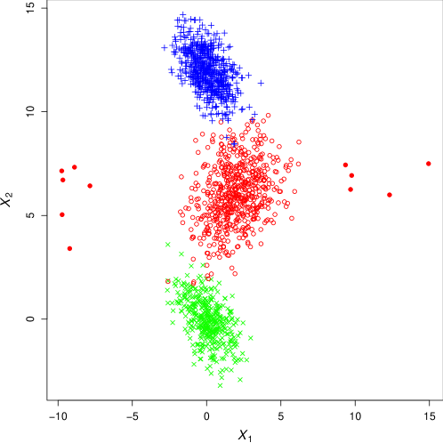
Figure 2: Synthetic data: scatter plot with colors and shapes representing the different clusters. Outliers are denoted by bullets.

Table 1 shows the obtained ER and ARI values. All of the methods have a similar classification performance.

	MNM	M$t$M	MS$t$M	MCNM	MSCNM
ER	0.009	0.010	0.014	0.009	0.009
ARI	0.972	0.97	0.958	0.972	0.974

Table 1: Synthetic data: ER and ARI values for the competing mixture models with $k=3$ components

Table 2 reports the number of false positives (i.e. the number of points incorrectly detected as outliers) related to the outlier detection rule of the competing robust methods. We can note how the detection rule from the MSCNM is the only one that does not incorrectly label good points as outliers.

M$t$M	MS$t$M	MCNM	MSCNM
93	35	1	0

Table 2: Synthetic data: number of points incorrectly identified as outliers by some robust procedures

On the contrary, M$t$Ms and MS$t$MS detect many more outliers than there should be.

For the MSCNM, the estimates of the parameters $\boldsymbol{\mu}_{j}$ and $\boldsymbol{\Sigma}_{j}$, $j=1,2,3$, are very close to the true ones. Particular attention has to be devoted to evaluate the estimates of $\boldsymbol{\alpha}_{j}$ and $\boldsymbol{\eta}_{j}$, $j=1,2,3$. Clusters 1 and 3 do not have outliers ($\widehat{\boldsymbol{\alpha}}_{1}=\widehat{\boldsymbol{\alpha}}_{3}=\left(0.999,0.999\right)^{\top}$), and cluster 2, with $\widehat{\boldsymbol{\alpha}}_{2}=\left(0.979,0.999\right)^{\top}$, has about 2% of outliers and only on the first dimension; in the same group, the bidimensional degree of contamination is $\widehat{\boldsymbol{\eta}}_{2}=\left(18.384,1.001\right)^{\top}$. The first value of $\widehat{\boldsymbol{\eta}}_{2}$ highlights how the corresponding MSCN mixture component distribution needs to make its tails heavier, on the first dimension only, to accommodate the outliers included into the data. The remaining bidimensional degrees of contamination are $\widehat{\boldsymbol{\eta}}_{1}=\widehat{\boldsymbol{\eta}}_{3}=\left(1.001,1.001\right)^{\top}$. Finally, it is of interest to note that similar results are obtained for the MCNM with reference to $\boldsymbol{\mu}_{j}$ and $\boldsymbol{\Sigma}_{j}$, $j=1,2,3$. Also, in this case, the second mixture component is devoted to accommodate the outliers, with $\widehat{\alpha}_{2}=0.978$ and $\widehat{\eta}_{2}=15.096$. However, the "omnibus" value of $\widehat{\eta}_{2}$ is not able to clarify that there are outliers on the first dimension only.

5.2 Wholesale Data

The real data analysis considers the wholesale data set, which is freely available on the UCI machine learning repository at https://archive.ics.uci.edu/ml/datasets/wholesale+customers. The data set originates from a larger database (see Abreu, 2011) and contains information about the annual spending, in monetary units, on $d=6$ products for $n=440$ customers of a wholesale merchant in Portugal. The product categories are: fresh, milk, grocery, frozen, detergents paper (DP), and delicatessen. The data set also contains two nominal variables: region (Lisboa, Porto, or other) and channel (hotel/restaurant/café or retail). There is no distinguishable difference in consumption among the regions, but there is a distinguishable difference between channels. The objective of this analysis is to segment the customers based on their spending and to compare these segments to the channel.

Figure 3 shows the scatter plot matrix of the standardized data, with each color and symbol representing a different channel.

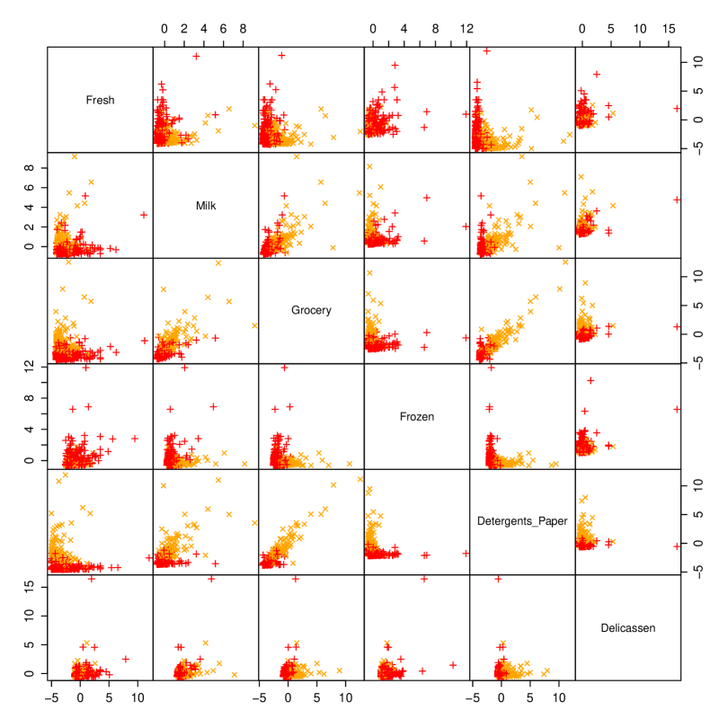
Figure 3: Wholesale data: scatter plot matrix with classification of the customers based on the channel ($\times$ and $+$ denote retail and horeca channels, respectively).

There is an high level of overlap between groups, and there are different number of outliers per variable.

The competing models were fitted with $k=2$ components, and $k$-medoids was used as the initialization strategy for all the fitting algorithms. Table 3 shows the ER for each model. The MCNM gives the best performance with $\text{ER}=0.18$ and $\text{ARI}=0.39$.

	MNM	M$t$M	MS$t$M	MCNM	MSCNM
ER	0.202	0.220	0.209	0.248	0.177
ARI	0.341	0.311	0.302	0.252	0.395

Table 3: Wholesale data: ER and ARI values for the competing mixture models with $k=2$ components

Table 4 shows the number of outliers per dimension detected using the fitted MSCNM. Grocery, fresh, and delicatessen have the higher number of outliers.

Fresh	Milk	Grocery	Frozen	DP	Delicatessen
5	6	2	2	1	4

Table 4: Wholesale data: number of outliers per dimension detected by the MSCN mixture with $k=2$ components

Some of the estimated parameters from the fitted MSCNM with $k=2$ components can help in the interpretation of the results. Table 5 shows the estimates of $\boldsymbol{\mu}_{j}$, $\boldsymbol{\alpha}_{j}$, and $\boldsymbol{\eta}_{j}$ for each cluster.

	Fresh	Milk	Grocery	Frozen	DP	Delicatessen
$\boldsymbol{\mu}_{1}$	0.049	-0.342	-0.387	0.048	-0.369	-0.141
$\boldsymbol{\alpha}_{1}$	0.983	0.982	0.961	0.990	0.990	0.992
$\boldsymbol{\eta}_{1}$	24.486	13.552	2.097	1.001	1.001	1.001
$\boldsymbol{\mu}_{2}$	-0.215	0.935	1.127	-0.228	1.132	0.366
$\boldsymbol{\alpha}_{2}$	0.987	0.941	0.971	0.970	0.947	0.946
$\boldsymbol{\eta}_{2}$	30.307	8.816	16.317	31.962	5.777	12.155

Table 5: Wholesale data: some of the estimated parameters from the MSCN mixture with $k=2$ components

The customers in cluster one spend more for fresh and frozen products. In this cluster, there is a 4% outlying spending in grocery and 2% in fresh and milk. The outliers for fresh and milk are further away from the bulk of the spending for this group when compared to the outliers for grocery. The customers in cluster two are those spending more for milk, grocery, detergent paper, and delicatessen categories. There are more outliers in this cluster, and they are generally farther away from the centers when compared to cluster one, with the exception of milk.

6 Conclusions

The multivariate contaminated normal (MCN) distribution, with respect to the classical multivariate normal (MN) distribution, has two additional parameters, $\alpha$ and $\eta$, denoting the proportion of good data and the degree of contamination, respectively. In this paper, we derived the multiple-scaled contaminated normal (MSCN) distribution to allow $\alpha$ and $\eta$ to vary across the $d$ dimensions. We referred to the possibility to work dimension-by-dimension using the adjective "directional." The MSCN distribution was obtained following the strategy of Forbes and Wraith (2014). In our setting, such a strategy was roughly based on two key elements: (1) the eigen decomposition of the scale matrix $\boldsymbol{\Sigma}$ of the MCN distribution and (2) the introduction of a multidimensional Bernoulli variable indicating whether a point is good or bad separately for each dimension. The MSCN distribution has a closed-form representation and depends on $2d$ additional parameters, with respect to the MN distribution, which represent the proportion of good data and the degree of contamination on each dimension. Advantageously, the MSCN distribution permits directional robust estimation of the mean vector and covariance matrix of the MN distribution and also gives automatic directional detection of bad points in the same natural way as observations are typically assigned to the groups in the finite mixture models context, i.e., based on the posterior probabilities of being good or bad points in each dimension. With respect to the former advantage, as an example, the estimator in (15) of the mean for the generic $h$th dimension, $h=1,\ldots,d$, is a weighted mean in which the weights reduce the impact of bad points (in that dimension) in the estimation.

The MSCN distribution was applied to robust model-based clustering by introducing mixtures of MSCN distributions; a variant of the EM algorithm was also described to obtain ML estimates for the mixture parameters. In the real and artificial data analyses of Section 5, we demonstrated the good behavior of our directional contaminated approach when compared to mixtures of the following distributions: MN, M$t$, MCN, and MS$t$.

Future work will focus on the following avenues:

• Our mixture model implies symmetric distributions for each cluster which, under specific empirical settings, could be rather restrictive. This is justified by the fact that non-symmetric distributions can be approximated quite well by a mixture of several basic symmetric distributions. While this can be very helpful for modeling purposes, it can be misleading when dealing with clustering and classification applications because one cluster may be represented by more than one mixture component simply because it has, in fact, a skewed distribution. To overcome this issue, we could extend our MSCN distribution with the aim of introducing skewness; the resulting model could be used to define the components of a mixture. Examples of competing approaches in this directions are given in Franczak et al. (2015) and Tortora et al. (2018).

• In the fashion of McLachlan and Peel (2000), McLachlan et al. (2003), and McNicholas and Murphy (2008) for mixtures of MN distributions; McLachlan et al. (2007) and Andrews and McNicholas (2011) for mixtures of M$t$ distributions; and Punzo and McNicholas (2014) for mixtures of MCN distributions, parsimony and dimension reduction could be obtained by exploiting local factor analyzers.

References

- Abreu (2011) Abreu, N. G. (2011). Analise do perfil do cliente Recheio e desenvolvimento de um sistema promocional. Ph.D. thesis, Mestrado em Marketing, ISCTE-IUL, Lisbon.
- Aitken (1926) Aitken, A. C. (1926). On Bernoulli's numerical solution of algebraic equations. In Proceedings of the Royal Society of Edinburgh, volume 46, pages 289–305.
- Aitkin and Wilson (1980) Aitkin, M. and Wilson, G. T. (1980). Mixture models, outliers, and the EM algorithm. Technometrics, 22(3), 325–331.
- Alqallaf et al. (2009) Alqallaf, F., Van Aelst, S., Yohai, V. J., Zamar, R. H., et al. (2009). Propagation of outliers in multivariate data. The Annals of Statistics, 37(1), 311–331.
- Andrews et al. (2018) Andrews, J., Wickins, J., Boers, N., and McNicholas, P. (2018). teigen: An R package for model-based clustering and classification via the multivariate t distribution. Journal of Statistical Software, 83(7), 1–32.
- Andrews and McNicholas (2011) Andrews, J. L. and McNicholas, P. D. (2011). Extending mixtures of multivariate -factor analyzers. Statistics and Computing, 21(3), 361–373.
- Bagnato and Punzo (2013) Bagnato, L. and Punzo, A. (2013). Finite mixtures of unimodal beta and gamma densities and the -bumps algorithm. Computational Statistics, 28(4), 1571–1597.
- Bagnato et al. (2017) Bagnato, L., Punzo, A., and Zoia, M. G. (2017). The multivariate leptokurtic-normal distribution and its application in model-based clustering. Canadian Journal of Statistics, 45(1), 95–119.
- Berkane and Bentler (1988) Berkane, M. and Bentler, P. M. (1988). Estimation of contamination parameters and identification of outliers in multivariate data. Sociological Methods & Research, 17(1), 55–64.
- Biernacki et al. (2003) Biernacki, C., Celeux, G., and Govaert, G. (2003). Choosing starting values for the EM algorithm for getting the highest likelihood in multivariate Gaussian mixture models. Computational Statistics & Data Analysis, 41(3-4), 561–575.
- Bock (2002) Bock, H. H. (2002). Clustering methods: From classical models to new approaches. Statistics in Transition, 5(5), 725–758.
- Böhning (2000) Böhning, D. (2000). Computer-Assisted Analysis of Mixtures and Applications: Meta-analysis, Disease Mapping and Others, volume 81 of Monographs on Statistics and Applied Probability. Chapman & Hall/CRC, London.
- Böhning et al. (1994) Böhning, D., Dietz, E., Schaub, R., Schlattmann, P., and Lindsay, B. (1994). The distribution of the likelihood ratio for mixtures of densities from the one-parameter exponential family. Annals of the Institute of Statistical Mathematics, 46(2), 373–388.
- Box (1980) Box, G. E. P. (1980). Sampling and bayes' inference in scientific modelling and robustness. Journal of the Royal Statistical Society: Series A (Statistics in Society), 143(4), 383–430.
- Box and Tiao (2011) Box, G. E. P. and Tiao, G. C. (2011). Bayesian Inference in Statistical Analysis. Wiley Classics Library. Wiley.
- Browne et al. (2018) Browne, R. P., ElSherbiny, A., and McNicholas, P. D. (2018). mixture: Finite Gaussian Mixture Models for Clustering and Classification. R package Version 1.5 (2018-02-13).
- Dang et al. (2015) Dang, U. J., Browne, R. P., and McNicholas, P. D. (2015). Mixtures of multivariate power exponential distributions. Biometrics, 71(4), 1081–1089.
- Davies and Gather (1993) Davies, L. and Gather, U. (1993). The identification of multiple outliers. Journal of the American Statistical Association, 88(423), 782–792.
- Dempster et al. (1977) Dempster, A., Laird, N., and Rubin, D. (1977). Maximum likelihood from incomplete data via the EM algorithm. Journal of the Royal Statistical Society. Series B (Methodological), 39(1), 1–38.
- Devlin et al. (1981) Devlin, S. J., Gnanadesikan, R., and Kettenring, J. R. (1981). Robust estimation of dispersion matrices and principal components. Journal of the American Statistical Association, 76(374), 354–362.
- Farcomeni (2014a) Farcomeni, A. (2014a). Robust constrained clustering in presence of entry-wise outliers. Technometrics, 56(1), 102–111.
- Farcomeni (2014b) Farcomeni, A. (2014b). Snipping for robust -means clustering under component-wise contamination. Statistics and Computing, 24(6), 907–919.
- Farcomeni and Greco (2016) Farcomeni, A. and Greco, L. (2016). Robust Methods for Data Reduction. CRC Press.
- Fessler and Hero (1994) Fessler, J. A. and Hero, A. O. (1994). Space-alternating generalized expectation-maximization algorithm. IEEE Transactions on Signal Processing, 42(10), 2664–2677.
- Forbes and Wraith (2014) Forbes, F. and Wraith, D. (2014). A new family of multivariate heavy-tailed distributions with variable marginal amounts of tailweight: application to robust clustering. Statistics and Computing, 24(6), 971–984.
- Fraley and Raftery (1998) Fraley, C. and Raftery, A. E. (1998). How many clusters? Which clustering method? Answers via model-based cluster analysis. Computer Journal, 41(8), 578–588.
- Franczak et al. (2015) Franczak, B. C., Tortora, C., Browne, R. P., and McNicholas, P. D. (2015). Unsupervised learning via mixtures of skewed distributions with hypercube contours. Pattern Recognition Letters, 58(1), 69–76.
- Gallegos and Ritter (2009) Gallegos, M. T. and Ritter, G. (2009). Trimmed ML estimation of contaminated mixtures. Sankhyā: The Indian Journal of Statistics A, 71(2), 164–220.
- Gómez et al. (2003) Gómez, E., Gómez-Villegas, M. A., and Marín, J. M. (2003). A survey on continuous elliptical vector distributions. Revista Matemática Complutense, 16(1), 345–361.
- Gómez-Villegas et al. (2011) Gómez-Villegas, M. A., Gómez-Sánchez-Manzano, E., Maín, P., and Navarro, H. (2011). The effect of non-normality in the power exponential distributions. In L. Pardo, N. Balakrishnan, and M. A. Gil, editors, Modern Mathematical Tools and Techniques in Capturing Complexity, Understanding Complex Systems, pages 119–129. Springer-Verlag, Berlin Heidelberg.
- Hogg (1974) Hogg, R. V. (1974). Adaptive robust procedures: A partial review and some suggestions for future applications and theory. Journal of the American Statistical Association, 69(348), 909–923.
- Hubert and Arabie (1985) Hubert, L. and Arabie, P. (1985). Comparing partitions. Journal of classification, 2(1), 193–218.
- Karlis and Xekalaki (2003) Karlis, D. and Xekalaki, E. (2003). Choosing initial values for the EM algorithm for finite mixtures. Computational Statistics & Data Analysis, 41(3–4), 577–590.
- Kaufman and Rousseeuw (1990) Kaufman, L. and Rousseeuw, P. J. (1990). Partitioning around medoids (program PAM). Finding groups in data: an introduction to cluster analysis, pages 68–125.
- Kotz and Nadarajah (2004) Kotz, S. and Nadarajah, S. (2004). Multivariate -Distributions and Their Applications. Cambridge University Press, Cambridge.
- Lange et al. (1989) Lange, K. L., Little, R. J. A., and Taylor, J. M. G. (1989). Robust statistical modeling using the distribution. Journal of the American Statistical Association, 84(408), 881–896.
- Lindsay (1995) Lindsay, B. (1995). Mixture Models: Theory, Geometry and Applications, volume 5. NSF-CBMS Regional Conference Series in Probability and Statistics, Institute of Mathematical Statistics, Hayward, California.
- Little (1988) Little, R. J. A. (1988). Robust estimation of the mean and covariance matrix from data with missing values. Applied Statistics, 37(1), 23–38.
- Liu and Rubin (1994) Liu, C. and Rubin, D. B. (1994). The ECME algorithm: a simple extension of EM and ECM with faster monotone convergence. Biometrika, 81(4), 633–648.
- Maechler et al. (2018) Maechler, M., Rousseeuw, P., Struyf, A., and Hubert, M. (2018). cluster: "Finding Groups in Data": Cluster Analysis Extended Rousseeuw et al. R package Version 2.0.7-1 (2018-04-09).
- Maronna (1976) Maronna, R. A. (1976). Robust -estimators of multivariate location and scatter. The Annals of Statistics, 4(1), 51–67.
- Maronna and Yohai (2014) Maronna, R. A. and Yohai, V. J. (2014). Robust Estimation of Multivariate Location and Scatter. John Wiley & Sons.
- Maruotti and Punzo (2017) Maruotti, A. and Punzo, A. (2017). Model-based time-varying clustering of multivariate longitudinal data with covariates and outliers. Computational Statistics & Data Analysis, 113, 475–496.
- Mazza and Punzo (2018) Mazza, A. and Punzo, A. (2018). Mixtures of multivariate contaminated normal regression models. Statistical Papers. https://doi.org/10.1007/s00362-017-0964-y.
- McLachlan and Krishnan (2007) McLachlan, G. and Krishnan, T. (2007). The EM algorithm and extensions, volume 382 of Wiley Series in Probability and Statistics. John Wiley & Sons, New York, second edition.
- McLachlan and Basford (1988) McLachlan, G. J. and Basford, K. E. (1988). Mixture models: Inference and Applications to clustering. Marcel Dekker, New York.
- McLachlan and Peel (1998) McLachlan, G. J. and Peel, D. (1998). Robust cluster analysis via mixtures of multivariate -distributions. In A. Amin, D. Dori, P. Pudil, and H. Freeman, editors, Advances in Pattern Recognition, volume 1451 of Lecture Notes in Computer Science, pages 658–666. Springer Berlin - Heidelberg.
- McLachlan and Peel (2000) McLachlan, G. J. and Peel, D. (2000). Finite Mixture Models. John Wiley & Sons, New York.
- McLachlan et al. (2003) McLachlan, G. J., Peel, D., and Bean, R. W. (2003). Modelling high-dimensional data by mixtures of factor analyzers. Computational Statistics & Data Analysis, 41(3), 379–388.
- McLachlan et al. (2007) McLachlan, G. J., Bean, R. W., and Ben-Tovim Jones, L. (2007). Extension of the mixture of factor analyzers model to incorporate the multivariate -distribution. Computational Statistics & Data Analysis, 51(11), 5327–5338.
- McNicholas (2016) McNicholas, P. D. (2016). Mixture Model-Based Classification. Chapman and Hall/CRC Press, Boca Raton.
- McNicholas and Murphy (2008) McNicholas, P. D. and Murphy, T. B. (2008). Parsimonious Gaussian mixture models. Statistics and Computing, 18(3), 285–296.
- McNicholas et al. (2010) McNicholas, P. D., Murphy, T. B., McDaid, A. F., and Frost, D. (2010). Serial and parallel implementations of model-based clustering via parsimonious Gaussian mixture models. Computational Statistics & Data Analysis, 54(3), 711–723.
- Meng and van Dyk (1997) Meng, X.-L. and van Dyk, D. (1997). The EM algorithm – an old folk-song sung to a fast new tune. Journal of the Royal Statistical Society: Series B (Statistical Methodology), 59(3), 511–567.
- Peel and McLachlan (2000) Peel, D. and McLachlan, G. J. (2000). Robust mixture modelling using the distribution. Statistics and Computing, 10(4), 339–348.
- Punzo and Maruotti (2016) Punzo, A. and Maruotti, A. (2016). Clustering multivariate longitudinal observations: The contaminated Gaussian hidden Markov model. Journal of Computational and Graphical Statistics, 25(4), 1097–1116.
- Punzo and McNicholas (2014) Punzo, A. and McNicholas, P. D. (2014). Robust high-dimensional modeling with the contaminated Gaussian distribution. arXiv.org e-print 1408.2128, available at: http://arxiv.org/abs/1408.2128.
- Punzo and McNicholas (2016) Punzo, A. and McNicholas, P. D. (2016). Parsimonious mixtures of multivariate contaminated normal distributions. Biometrical Journal, 58(6), 1506–1537.
- Punzo and McNicholas (2017) Punzo, A. and McNicholas, P. D. (2017). Robust clustering in regression analysis via the contaminated Gaussian cluster-weighted model. Journal of Classification, 34(2), 249–293.
- Punzo et al. (2018) Punzo, A., Mazza, A., and McNicholas, P. (2018). ContaminatedMixt: An R package for fitting parsimonious mixtures of multivariate contaminated normal distributions. Journal of Statistical Software, 85(10), 1–25.
- Rand (1971) Rand, W. M. (1971). Objective criteria for the evaluation of clustering methods. Journal of the American Statistical Association, 66, 846–850.
- R Core Team (2018) R Core Team (2018). R: A Language and Environment for Statistical Computing. R Foundation for Statistical Computing, Vienna, Austria.
- Ritter (2015) Ritter, G. (2015). Robust Cluster Analysis and Variable Selection, volume 137 of Chapman & Hall/CRC Monographs on Statistics & Applied Probability. CRC Press.
- Rousseeuw and Leroy (2005) Rousseeuw, P. J. and Leroy, A. M. (2005). Robust Regression and Outlier Detection, volume 589 of Wiley Series in Probability and Statistics. Wiley.
- Subedi et al. (2013) Subedi, S., Punzo, A., Ingrassia, S., and McNicholas, P. D. (2013). Clustering and classification via cluster-weighted factor analyzers. Advances in Data Analysis and Classification, 7(1), 5–40.
- Subedi et al. (2015) Subedi, S., Punzo, A., Ingrassia, S., and McNicholas, P. D. (2015). Cluster-weighted -factor analyzers for robust model-based clustering and dimension reduction. Statistical Methods & Applications, 24(4), 623–649.
- Tortora et al. (2018) Tortora, C., Franczak, B., Browne, R., and McNicholas, P. (2018). A mixture of coalesced generalized hyperbolic distributions. Journal of Classification, (accepted).
- Tukey (1960) Tukey, J. W. (1960). A survey of sampling from contaminated distributions. In I. Olkin, editor, Contributions to Probability and Statistics: Essays in Honor of Harold Hotelling, Stanford Studies in Mathematics and Statistics, chapter 39, pages 448–485. Stanford University Press, California.
- Zhang and Liang (2010) Zhang, J. and Liang, F. (2010). Robust clustering using exponential power mixtures. Biometrics, 66(4), 1078–1086.