Higher-order modified Starobinsky inflation

Abstract

An extension of the Starobinsky model is proposed. Besides the usual Starobinsky Lagrangian, a term proportional to the derivative of the scalar curvature, $\nabla_{\mu}R\nabla^{\mu}R$, is considered. The analyzis is done in the Einstein frame with the introduction of a scalar field and a vector field. We show that inflation is attainable in our model, allowing for a graceful exit. We also build the cosmological perturbations and obtain the leading-order curvature power spectrum, scalar and tensor tilts and tensor-to-scalar ratio. The tensor and curvature power spectrums are compared to the most recent observations from BICEP2/Keck collaboration. We verify that the scalar-to-tensor rate $r$ can be expected to be up to three times the values predicted by Starobinsky model.

I Introduction

As is well known, the Starobinsky model is currently the most promising one for describing the cosmological inflation Starobinski1980 . Historically, several approaches were proposed exploring different physical aspects for describing the first stages of the universe Starobinski1980 ; Starobinski1979 ; Starobinsky1979a ; Sato1981 ; Guth1981 . The hypothesis of an inflationary universe driven by an scalar field was proposed in 1981 Sato1981 ; Guth1981 and provided an ingenious apparatus to solve, with only one mechanism, three disturbing problems of the standard big bang cosmology, namely the horizon, flatness and magnetic monopole problems. As a bonus, the large-scale structure can also be explained in this scenario. Although it is remarkable that this proposition could solve these problems at once, other complications arose, like the absence of a smooth transition from a de Sitter-like expansion to a decelerated Friedmann-Lemaître-Robertson-Walker (FLRW) one (a shortcoming dubbed as “graceful exit problem”). This motivated the proposition of alternative models (for instance, Linde1982 ; Linde1983 ; Steinhardt1982 ; Lucchin1985 ; Steinhardt1989 ) which solved the graceful exit problem at the cost of imposing a fine-tuning on the effective potential parameters Steinhardt1989 ; Steinhardt1993 . So the search for a consistent inflation model continued to strive for accomplishing some specific goals Steinhardt1993 : (i) providing a mechanism to drive the universe through a phase transition from a false vacuum to a true vacuum state, (ii) generating a brief period of exponential-like growth for the scale factor, and (iii) stipulating a smooth ending for the highly accelerated growth (graceful exit) thus allowing for the universe to reheat and enter a period of decelerated FLRW expansion.

A plethora of models were proposed suggesting the existence of a single scalar field (the “inflaton”) or multiple scalar fields Linde1994 ; Wand2008 (see also Basset2006 and references therein) that would drive the inflationary process. These models essentially consist of matter fields evolving in a curved spacetime described by general relativity (GR).

A different category of inflationary models, which is of particular interest here, is composed of those assuming modifications on the underlying theory of gravitation (i.e. GR). The $f\left(R\right)$ theories of gravity are perhaps the most explored class of modified gravity theories in the literature. An important feature of $f\left(R\right)$ theories lies on the fact that they are proven to be equivalent to scalar-tensor theories Faraoni2010 ; NojiriOdintsov2011 ; Capozziello2011 . This is very useful since the techniques developed for treating inflation models with scalar fields are applicable for an $f\left(R\right)$ theory when it is considered on its equivalent scalar-tensor form. It is important to recall that the scalar-tensor theory can be analyzed both in Jordan and Einstein frames. Although these frames are related by a conformal transformation, the analyzis of scalar-tensor models on non-minimal inflationary contexts may lead to different predictions in each case Karam2017 ; Shokri2017 .

Several inflation models have been proposed in the context of $f\left(R\right)$ gravity Amin2016 ; Artymoski2016 ; Elizalde2011 ; Brooker2016 ; Odintsov2015 ; Sadeghi2015 ; Asaka2016 ; Nojiri:2017ncd ; Fabris2017 , the most iconic one being the Starobinsky model Starobinski1980 ; Starobinski1979 ; Starobinsky1979a , which modifies the gravitational Lagrangian by adding to the usual Einstein-Hilbert Lagrangian a term proportional to the square of the scalar curvature, $L=R+aR^{2}$. This inflationary model is characterized by being simultaneously minimal in its new features and especially favoured by the most recent data from Planck satellite Calmet2016 . For instance, Starobinsky’s model predicts a tensor-to-scalar ratio $r<0.0048$ for a number of e-folds greater than $50$ (in a very conservative estimation) while Planck data Planck2018 suggests $r<0.064$ in the best scenario. This is one example of how superbly compatible with experimental data Starobinsky’s model is. However, this difference in order of magnitude in the estimation of $r$ (due to the not yet so precise measurement of this parameter) and the one predicted by the Starobinsky model still allows other models to be compatible with the data. In particular, those models that do not predict a very low production of primordial gravitational waves cannot be discarded until a precision of order $10^{-3}$ for the estimation of $r$ is finally achieved.

It is interesting to note that in the context of $f\left(R\right)$ Lagrangians terms proportional to $R^{n},\,n\geq 3$ are apparently suppressed Huang2014 . Hence, analytical functions of $R$ would only give contributions equivalent to Starobinky’s. In order to generalize the $f\left(R\right)$ models in the inflationary context other categories of modified gravity theories are taken into account, for instance those with Lagrangians containing the Gauss-Bonnet invariant and/or the Weyl tensor Starobinsky1987 ; Clunan2009 ; Capozzielo2015 ; Odintsov2015a ; Sebastiani2015 ; Ivanov2016 ; Salvio2017 . Some applications considering both inflationary scalar field and modified theory of gravity can also be found in the literature Starobinsky1985 ; Starobinsky1991 ; Weinberg2008 ; Baumann2016 with some interesting results, e.g. vector fields contribution should no longer be ignored in the presence of a (square) Weyl term in the Lagrangian Deruelle2010 .

Another category of modified gravity is composed of theories with Lagrangians containing derivatives of the curvature tensors (Riemann, Ricci, scalar curvature and so forth), which lead to field equations with derivatives of the metric of order higher than four. They are usually motivated in the context of quantum gravity and can be separated in two sub-categories: (i) theories with infinite derivatives of curvature Biswas2012 ; Biswas2015 ; Biswas2017 ; Modesto2014 ; Modesto2017 ; Shapiro2015 and (ii) theories with finite derivatives of curvature Asorey1992 ; Accioly2017 ; ModestoShapiro2016 ; Shapiro2014 ; Shapiro2014a ; Decanini2007 ; NosEPJC2008 . While the latter can exhibit (super-)renormalizability and locality, they are usually plagued with ghosts; the former, on their turn, may be ghost-free but present non-locality ModestoShapiro2016 . Applications of both approaches to inflationary context are found in the literature Berkin1990 ; Gottlober1990 ; Gottlober1991 ; Amendola1993 ; Iihoshi2011 ; Castellanos2018 ; Diamandis2017 ; Koshelev2016 ; Koshelev2018 ; Edholm2017 ; Chialva2015 . In particular, theories with an infinite number of derivatives are able to modify the tensor-to-scalar ratio Koshelev2016 ; Koshelev2018 ; Edholm2017 .

However, if one wants to keep locality, then theories with a finite number of derivatives are in order. As has been shown in Ref. Wands1994 , one can substitute the extra degrees of freedom associated to higher derivatives by auxiliary scalar fields in a particular class of finite higher order theory. In the case of sixth-order derivative equations for the metric, inflation is carried out by two scalar fields Berkin1990 ; Gottlober1991 ; Amendola1993 ; Iihoshi2011 ; Castellanos2018 . A new approach to deal with higher derivative Lagrangians has been proposed NosPRD2016 where the extra degrees of freedom arising from higher order contribution are replaced by auxiliary tensor fields instead of scalar fields only. This approach (in Jordan frame) is applicable for the class of higher order theories that is regular in the sense discussed in Ref. NosPRD2016 . That paper verified that the Lagrangian $L=R+aR^{2}+bR\square R$ analyzed in Refs. Gottlober1990 ; Iihoshi2011 can be equivalently described by a Lagrangian containing a scalar field and a vector field (instead of two scalar fields). The study of the field equation demonstrated that this vector field has only one (unconstrained) degree of freedom, showing consistency between the results in NosPRD2016 and Gottlober1990 ; Iihoshi2011 ; Castellanos2018 .

In the present work, an inflationary model constructed by the addition a higher order term of the type $\nabla_{\mu}R\nabla^{\mu}R$ to the Starobinsky action is proposed. The model is described in the Einstein frame, within the framework presented in Ref. Nos2018 . Accordingly, the extra degrees of freedom are given by a scalar and by a vector field. In this context, the scalar field plays the role of the usual Starobinsky inflation while the vector field produces corrections to Starobinsky’s inflation. The study of background dynamics is done under conditions that allow for an inflationary attractor regime obeying slow-roll conditions. The perturbative analyzis up to slow-roll regime leading order is also performed showing how the term $\nabla_{\mu}R\nabla^{\mu}R$ changes the predictions of Starobinsky inflation.

The paper is organized as follows: In Section II, we propose the modified gravity action and obtain the field equation in terms of the metric and the auxiliary fields. Next, in Section III, we study the background equations and show that an inflationary regime is attainable in our model. Section IV is devoted to the analyzis of the perturbed cosmological equations, whose solutions are evaluated in Section V. Finally, the cosmological parameters are determined in Section VI. Section VII is dedicated to the discussions of the main results.

II Modified gravity action

Starobinsky gravity Starobinski1980 , described by the action

$$S_{\text{Sta}}=\frac{M_{Pl}^{2}}{2}\int d^{4}x\sqrt{-g}\left[R+\frac{1}{2\kappa_{0}}R^{2}\right],$$ (1)

emerges nowadays as the most promising model for the description of the inflationary paradigm. Among the class of minimalist inflationary models, i.e. those composed of a single parameter Martin2014 , Starobinsky inflation is the one that best fits the observations of the CMB anisotropies Planck2018 . Besides, from a theoretical point of view, this model has an excellent motivation since quadratic terms involving the Riemann tensor arise naturally in a bottom-up approach to the quantization of gravitation Stelle1977 ; Asorey1992 ; Biswas2012 .

For the reasons given in the previous section, it is reasonable to expect that $S_{\text{Sta}}$ is not a fundamental action for gravity in spite of the success of Starobinsky inflation. Therefore, corrections to $S_{\text{Sta}}$ should exist. The first corrections to be considered in a context of increasing energy scales are those of the same order of $R^{2}$, i.e. those of the kind $R_{\mu\nu}R^{\mu\nu}$. On the one hand, the addition of this term to the action (1) makes gravitation a renormalizable theory; on the other hand, it introduces ghosts, rendering the quantization process questionable Desser1974 ; Stelle1977 .

The next order of correction in action $S_{\text{Sta}}$ is composed by terms of the type

$$\left(R_{\ast\ast\ast\ast}\right)^{3}\text{ or }\left(\nabla^{\ast}R_{\ast\ast\ast\ast}\right)^{2},$$

where $R_{\ast\ast\ast\ast}$ represents the Riemann tensor or any of its contractions. Cubic terms of the type $\left(R_{\ast\ast\ast\ast}\right)^{3}$ are not essential for consistency in the standard quantization procedure since they do not affect the structure of the propagator Asorey1992 . Thus, for simplicity, we neglect the cubic corrections and take into account only the terms involving derivatives of curvature-based objects. Ref. NosEPJC2008 showed that there are only four distinct terms of the form $\left(\nabla^{\ast}R_{\ast\ast\ast\ast}\right)^{2}$, namely,

$$\nabla_{\mu}R\nabla^{\mu}R\text{; \ }\nabla_{\mu}R_{\alpha\beta}\nabla^{\mu}R^{\alpha\beta}\text{; \ }\nabla^{\mu}R^{\alpha\beta}\nabla_{\alpha}R_{\mu\beta}\text{ \ and }\nabla_{\rho}R_{\mu\nu\alpha\beta}\nabla^{\rho}R^{\mu\nu\alpha\beta}\text{.}$$

By using Bianchi identities, it is possible to verify that only two of the four terms above are independent (modulo cubic order terms). Therefore, the action integral with corrections to Einstein-Hilbert term up to second order is:

$$S_{2}=\frac{M_{Pl}^{2}}{2}\int d^{4}x\sqrt{-g}\left[R+\frac{1}{2\kappa_{0}}R^{2}+\frac{1}{2\kappa_{2}}R_{\mu\nu}R^{\mu\nu}+\frac{\beta_{0}}{2\kappa_{0}^{2}}\nabla_{\mu}R\nabla^{\mu}R+\frac{\beta_{2}}{2\kappa_{2}^{2}}\nabla_{\mu}R_{\alpha\beta}\nabla^{\mu}R^{\alpha\beta}\right],$$ (2)

where $\kappa_{i}$ are constants with square mass dimension and $\beta_{i}$ are dimensionless constants. This action presents interesting properties such as super-renormalizability Asorey1992 ; ModestoShapiro2016 and finiteness of the gravitational potential (weak field regime) at the origin AcciolyGiacchiniShapiro2016 . However, the presence of the massive spin-$2$ terms associated with $R_{\mu\nu}$ inevitably introduces ghosts into the theory.

It may be conjectured that the pathologies associated with ghosts (vacuum decay or unitarity loss Sbisa2014 ) can be controlled during the well-defined energy scales of inflation by making $S_{2}$ a consistent effective theory Fradkin1982 ; Buchbinder1989 . This type of approach was adopted in Refs. Clunan2009 ; Ivanov2016 ; Salvio2017 precisely to deal with inflationary models which contain the $R_{\mu\nu}R^{\mu\nu}$ term. Although this is a valid approach, in this work we will neglect both the spin-$2$ terms.

Based on the previous discussion, we start by considering a gravitational action that differs from $S_{\text{Sta}}$ by the addition of the higher-order term $\nabla_{\mu}R\nabla^{\mu}R$:

$$S_{g}=\frac{M_{Pl}^{2}}{2}\int d^{4}x\sqrt{-g}\left[R+\frac{1}{2\kappa_{0}}R^{2}+\frac{\beta_{0}}{2\kappa_{0}^{2}}\nabla_{\mu}R\nabla^{\mu}R\right].$$ (3)

Constant $\kappa_{0}$ sets the energy scale of the inflationary regime and $\beta_{0}$ is a measure of the deviation from Starobinsky inflation model. An important point to be emphasized is that Eq. (3) will be ghost-free if $\beta_{0}<0$ Hindawi1996 . Ref. Nos2018 has shown this action can be re-expressed in Einstein frame where a scalar field and a vector field play the role of the higher derivative terms:

$$S_{g}^{\prime\prime}=\int d^{4}x\sqrt{-\tilde{g}}\left\{\frac{M_{Pl}^{2}}{2}\tilde{R}-\frac{1}{2}\partial_{\rho}\tilde{\Phi}\tilde{\partial}^{\rho}\tilde{\Phi}-\frac{M_{Pl}^{2}}{2}e^{-2\sqrt{\frac{2}{3}}\frac{\tilde{\Phi}}{M_{Pl}}}\left(\frac{\kappa_{0}}{2}\Upsilon^{2}+\frac{1}{2}\frac{\beta_{0}}{\kappa_{0}^{2}}e^{-\sqrt{\frac{2}{3}}\frac{\tilde{\Phi}}{M_{Pl}}}\tilde{g}_{\mu\nu}\xi^{\nu}\xi^{\mu}\right)\right\},$$ (4)

where

$$\Upsilon\equiv\Upsilon\left(\tilde{\Phi},\partial\tilde{\Phi},\xi^{\mu},\partial\xi^{\mu}\right)\equiv e^{\sqrt{\frac{2}{3}}\frac{\tilde{\Phi}}{M_{Pl}}}+\frac{\beta_{0}}{\kappa_{0}^{2}}\tilde{\nabla}_{\mu}\xi^{\mu}-\frac{2}{M_{Pl}}\sqrt{\frac{2}{3}}\frac{\beta_{0}}{\kappa_{0}^{2}}\xi^{\rho}\partial_{\rho}\tilde{\Phi}-1,$$

with

$$\tilde{\Phi} \equiv M_{Pl}\sqrt{\frac{3}{2}}\ln\left(\frac{\partial f\left(\xi,\xi_{\mu}\right)}{\partial\xi}-\nabla_{\mu}\phi^{\mu}\right),$$

$$\phi^{\mu} \equiv\frac{\partial f}{\partial\xi_{\mu}}=\frac{\beta_{0}}{\kappa_{0}^{2}}\xi^{\mu}.$$

The effective “matter” field Lagrangian, i.e. the Lagrangian for the scalar and vector fields, now reads:

$$\mathcal{L}_{\text{eff}}=-\frac{1}{2}\partial_{\rho}\tilde{\Phi}\tilde{\partial}^{\rho}\tilde{\Phi}-\frac{M_{Pl}^{2}}{2}e^{-2\sqrt{\frac{2}{3}}\frac{\tilde{\Phi}}{M_{Pl}}}\left(\frac{\kappa_{0}}{2}\Upsilon^{2}+\frac{1}{2}\frac{\beta_{0}}{\kappa_{0}^{2}}e^{-\sqrt{\frac{2}{3}}\frac{\tilde{\Phi}}{M_{Pl}}}\tilde{g}_{\mu\nu}\xi^{\nu}\xi^{\mu}\right).$$ (5)

Lagrangian $\mathcal{L}_{\text{eff}}$ is used for evaluating the field equations for $\tilde{\Phi}$ and $\xi^{\mu}$, which are given respectively by

$$\tilde{\Box}\tilde{\Phi}+\sqrt{\frac{2}{3}}\frac{\kappa_{0}}{2}M_{Pl}e^{-2\sqrt{\frac{2}{3}}\frac{\tilde{\Phi}}{M_{Pl}}}\Upsilon\left(\Upsilon-e^{\sqrt{\frac{2}{3}}\frac{\tilde{\Phi}}{M_{Pl}}}\right)$$

$$+\frac{\beta_{0}}{\kappa_{0}^{2}}M_{Pl}\left[-\kappa_{0}\sqrt{\frac{2}{3}}\tilde{\nabla}_{\rho}\left(e^{-2\sqrt{\frac{2}{3}}\frac{\tilde{\Phi}}{M_{Pl}}}\Upsilon\xi^{\rho}\right)+\sqrt{\frac{2}{3}}\frac{3}{4}e^{-3\sqrt{\frac{2}{3}}\frac{\tilde{\Phi}}{M_{Pl}}}\tilde{\xi}_{\mu}\xi^{\mu}\right]=0,$$ (6)

and

$$\kappa_{0}\partial_{\rho}\Upsilon-e^{-\sqrt{\frac{2}{3}}\frac{\tilde{\Phi}}{M_{Pl}}}\tilde{\xi}_{\rho}=0,$$ (7)

where $\tilde{\xi}_{\mu}\equiv\tilde{g}_{\mu\nu}\xi^{\nu}$. These two equations can be combined to give:

$$\tilde{\Box}\tilde{\Phi}+\sqrt{\frac{2}{3}}\frac{\kappa_{0}}{2}M_{Pl}e^{-2\sqrt{\frac{2}{3}}\frac{\tilde{\Phi}}{M_{Pl}}}\Upsilon\left(e^{\sqrt{\frac{2}{3}}\frac{\tilde{\Phi}}{M_{Pl}}}-\Upsilon-2\right)-\frac{\beta_{0}}{\kappa_{0}^{2}}M_{Pl}\sqrt{\frac{2}{3}}\frac{1}{4}e^{-3\sqrt{\frac{2}{3}}\frac{\tilde{\Phi}}{M_{Pl}}}\tilde{\xi}_{\mu}\xi^{\mu}=0.$$ (8)

The field equation for $\tilde{g}^{\mu\nu}$ reads:

$$\tilde{G}_{\mu\nu}=\frac{1}{M_{Pl}^{2}}\tilde{T}_{\mu\nu}^{\left(\text{eff}\right)},$$

where

$$\tilde{T}_{\rho\sigma}^{\left(\text{eff}\right)} \equiv\frac{2}{\sqrt{-\tilde{g}}}\frac{\delta\left(\sqrt{-\tilde{g}}\mathcal{L}_{\text{eff}}\right)}{\delta\tilde{g}^{\rho\sigma}}$$

$$=\partial_{\rho}\tilde{\Phi}\partial_{\sigma}\tilde{\Phi}-\frac{M_{Pl}^{2}}{2}\frac{\beta_{0}}{\kappa_{0}^{2}}e^{-3\sqrt{\frac{2}{3}}\frac{\tilde{\Phi}}{M_{Pl}}}\tilde{\xi}_{\rho}\tilde{\xi}_{\sigma}+\tilde{g}_{\rho\sigma}\left[\mathcal{L}_{\text{eff}}+\frac{M_{Pl}^{2}}{2}\frac{\beta_{0}}{\kappa_{0}}\tilde{\nabla}_{\nu}\left(e^{-2\sqrt{\frac{2}{3}}\frac{\tilde{\Phi}}{M_{Pl}}}\Upsilon\xi^{\nu}\right)\right]$$ (9)

is the (effective) energy-momentum tensor.

Henceforth we shall omit the tilde for notation economy.

The effective energy-momentum tensor (9) is of the imperfect fluid type Nos2018 :

$$T_{\mu\nu}=\left(\varepsilon+p\right)u_{\mu}u_{\nu}+pg_{\mu\nu}+u_{\mu}q_{\nu}+u_{\nu}q_{\mu}+\pi_{\mu\nu},$$ (10)

where $p$ is the pressure, $\varepsilon$ is the energy density, $u_{\mu}$ is the four-velocity of the fluid element, $q_{\mu}$ is the heat flux vector and $\pi_{\mu\nu}$ is the viscous shear tensor; these quantities satisfy $q_{\mu}u^{\mu}=0,\,\pi_{\mu\nu}u^{\nu}=0,\,\pi_{\,\mu}^{\mu}=0,\,\pi_{\mu\nu}=\pi_{\nu\mu}$. In fact, Eqs. (9) and (10) are the same under the following identifications:

$$\varepsilon+p =-\partial^{\alpha}\Phi\partial_{\alpha}\Phi+\frac{M_{Pl}^{2}}{2}\frac{\beta_{0}}{\kappa_{0}^{2}}e^{-3\sqrt{\frac{2}{3}}\frac{\Phi}{M_{Pl}}}\xi_{\alpha}\xi^{\alpha},$$ (11)

$$u_{\mu} =\frac{1}{N}\left(\partial_{\mu}\Phi+\sqrt{\frac{M_{Pl}^{2}}{2}\frac{\beta_{0}}{\kappa_{0}^{2}}}e^{-\frac{3}{2}\sqrt{\frac{2}{3}}\frac{\Phi}{M_{Pl}}}\xi_{\mu}\right),$$ (12)

$$q_{\mu} =-\sqrt{\frac{M_{Pl}^{2}}{2}\frac{\beta_{0}}{\kappa_{0}^{2}}}e^{-\frac{3}{2}\sqrt{\frac{2}{3}}\frac{\Phi}{M_{Pl}}}N\left(\xi_{\mu}+\xi^{\alpha}u_{\alpha}u_{\mu}\right),$$ (13)

$$p =\mathcal{L}_{\text{eff}}+\frac{M_{Pl}^{2}}{2}\frac{\beta_{0}}{\kappa_{0}}\nabla_{\nu}\left(e^{-2\sqrt{\frac{2}{3}}\frac{\Phi}{M_{Pl}}}\Upsilon\xi^{\nu}\right),$$ (14)

$$\pi_{\mu\nu} =0,$$ (15)

with

$$N=\sqrt{-\left(\partial_{\alpha}\Phi+\sqrt{\frac{M_{Pl}^{2}}{2}\frac{\beta_{0}}{\kappa_{0}^{2}}}e^{-\frac{3}{2}\sqrt{\frac{2}{3}}\frac{\Phi}{M_{Pl}}}\xi_{\alpha}\right)\left(\partial^{\alpha}\Phi+\sqrt{\frac{M_{Pl}^{2}}{2}\frac{\beta_{0}}{\kappa_{0}^{2}}}e^{-\frac{3}{2}\sqrt{\frac{2}{3}}\frac{\Phi}{M_{Pl}}}\xi^{\alpha}\right)},$$ (16)

Hence, the fluid represented by Eq. (9) has no contribution from viscous shear components, which are null here. Notice that the heat flux vector exists solely due to the higher order term — were it absent, the theory would be reduced to Starobinsky’s model and, therefore, would be represented by a perfect fluid energy-momentum tensor. The above equations are specified in FLRW spacetime in the next section.

III Cosmological background equations

In order to analyze the action (4) for background cosmology, we consider: (i) a homogeneous and isotropic spacetime, (ii) a comoving reference frame ($u^{\mu}=\delta_{0}^{\mu}$), (iii) spherical coordinates for the space sector and (iv) null space curvature parameter ($k=0$). With these assumptions, the line element is FLRW metric:

$$ds^{2}=-dt^{2}+a^{2}\left(t\right)\left[dr^{2}+r^{2}d\Omega^{2}\right],$$

where $a\left(t\right)$ is the scale factor.

In this case, the Einstein tensor is diagonal and Einstein equations imply that the space components of the heat flux vector are null. Also, condition $q_{\mu}u^{\mu}=0$ imposes $q_{0}=0$ showing there is no heat flux for a homogeneous and isotropic spacetime. Einstein equations are then reduced to:

$$H^{2} =\frac{1}{3M_{Pl}^{2}}\varepsilon,$$ (17)

$$\frac{dH}{dt} =-\frac{1}{2M_{Pl}^{2}}\left(\varepsilon+p\right),$$ (18)

where $H\equiv\frac{1}{a}\frac{da}{dt}$ is the Hubble function. The energy density and pressure are given in terms of the auxiliary fields and their derivatives:

$$\varepsilon =\frac{1}{2}\left(\frac{d\Phi}{dt}\right)^{2}+\frac{1}{2}\frac{M_{Pl}^{2}}{2}\kappa_{0}\left(1-e^{-\sqrt{\frac{2}{3}}\frac{\Phi}{M_{Pl}}}\right)^{2}-\frac{1}{2}\frac{M_{Pl}^{2}}{2}\frac{\beta_{0}}{\kappa_{0}^{2}}e^{-3\sqrt{\frac{2}{3}}\frac{\Phi}{M_{Pl}}}\left(\xi^{0}\right)^{2}$$

$$-\frac{1}{2}\frac{M_{Pl}^{2}}{2}\kappa_{0}\left(\frac{\beta_{0}}{\kappa_{0}^{2}}\right)^{2}e^{-2\sqrt{\frac{2}{3}}\frac{\Phi}{M_{Pl}}}\left(\frac{d\xi^{0}}{dt}+3H\xi^{0}-\frac{2}{M_{Pl}}\sqrt{\frac{2}{3}}\xi^{0}\frac{d\Phi}{dt}\right)^{2},$$

and

$$\varepsilon+p=\left(\frac{d\Phi}{dt}\right)^{2}-\frac{M_{Pl}^{2}}{2}\frac{\beta_{0}}{\kappa_{0}^{2}}e^{-3\sqrt{\frac{2}{3}}\frac{\Phi}{M_{Pl}}}\left(\xi^{0}\right)^{2}.$$ (19)

For consistency, the auxiliary field $\Phi$ must also be homogenous and isotropic, so it can only be time-dependent. In this case, when the comoving frame is considered, the auxiliary vector field space components have to be null, which is consistent with the fact that the heat flux vector is also null. Notice that $\xi^{0}$ does not vanish and actually it is a dynamical quantity in FLRW background, as verified by the field equations (8) and (7):

$$\frac{d^{2}\Phi}{dt^{2}}+3H\frac{d\Phi}{dt}-\sqrt{\frac{2}{3}}\frac{\kappa_{0}}{2}M_{Pl}e^{-2\sqrt{\frac{2}{3}}\frac{\Phi}{M_{Pl}}}\Upsilon\left(e^{\sqrt{\frac{2}{3}}\frac{\Phi}{M_{Pl}}}-\Upsilon-2\right)-\frac{1}{4}\sqrt{\frac{2}{3}}\frac{\beta_{0}}{\kappa_{0}^{2}}M_{Pl}e^{-3\sqrt{\frac{2}{3}}\frac{\Phi}{M_{Pl}}}\left(\xi^{0}\right)^{2}=0,$$ (20)

and

$$\kappa_{0}\frac{d\Upsilon}{dt}+e^{-\sqrt{\frac{2}{3}}\frac{\tilde{\Phi}}{M_{Pl}}}\xi^{0}=0,$$ (21)

where

$$\Upsilon=e^{\sqrt{\frac{2}{3}}\frac{\Phi}{M_{Pl}}}-1+\frac{\beta_{0}}{\kappa_{0}^{2}}\left(\frac{d\xi^{0}}{dt}+3H\xi^{0}-\frac{2}{M_{Pl}}\sqrt{\frac{2}{3}}\xi^{0}\frac{d\Phi}{dt}\right).$$

The following step is to check whether the above equations are suitable to describe an inflationary regime. This is the analysis in the next subsection.

III.1 Analysis of the field equations: attractors

We work in phase space. It is convenient to define new dimensionless variables for the auxiliary fields:

$$X\equiv\sqrt{\frac{2}{3}}\frac{\Phi}{M_{Pl}}\text{, \ \ }Y\equiv\sqrt{\frac{2}{3}}\frac{\dot{\Phi}}{M_{Pl}}\text{, }\quad T\equiv\frac{\xi^{0}}{\kappa_{0}^{3/2}}\text{ \ \ and \ \ \ }S\equiv\frac{\dot{\xi}^{0}}{\kappa_{0}^{3/2}},$$ (22)

with

$$\bar{\partial}_{0}Q=\dot{Q}\equiv\frac{1}{\sqrt{\kappa_{0}}}\partial_{0}Q,$$ (23)

where $\bar{\partial}_{0}$ (and dot) denotes a dimensionless time derivative. A dimensionless Hubble function can also be defined:

$$h_{\kappa}\equiv\frac{H}{\sqrt{\kappa_{0}}}.$$ (24)

Then, FLRW equations, (17) and (18), become:

$$\dot{h}_{\kappa} =-\frac{1}{4}\left(3Y^{2}-\beta_{0}T^{2}e^{-3X}\right),$$ (25)

$$h_{k}^{2} =\frac{1}{12}\left[3Y^{2}+\left(1-e^{-X}\right)^{2}-\beta_{0}e^{-3X}T^{2}-\beta_{0}^{2}e^{-2X}\left(S+3h_{\kappa}T-2TY\right)^{2}\right].$$ (26)

Similarly, the auxiliary field equations (20) and (21) are rewritten as :

$$\dot{Y}+3h_{\kappa}Y+\frac{1}{3}e^{-X}\left(1-e^{-X}\right)-\frac{1}{6}\beta_{0}e^{-3X}T^{2}$$

$$+\frac{1}{3}\beta_{0}e^{-X}\left(S+3h_{\kappa}T-2YT\right)+\frac{1}{3}\beta_{0}^{2}e^{-2X}\left(S+3h_{\kappa}T-2YT\right)^{2}=0,$$ (27)

and

$$Ye^{X}+\beta_{0}\left(\dot{S}+3\dot{h}_{\kappa}T+3h_{\kappa}S-2SY-2\dot{Y}T\right)+e^{-X}T=0.$$ (28)

The quadratic equation (26) can be manipulated to express $h_{\kappa}$ in terms of the auxiliary fields $X,\,Y,\,T$ and $S$:

$$h_{\kappa} =\frac{-\frac{1}{2}\beta_{0}^{2}e^{-2X}T\left(S-2TY\right)}{2\left(1+\frac{3}{4}\beta_{0}^{2}e^{-2X}T^{2}\right)}$$

$$+\frac{\sqrt{\left(1+\frac{3}{4}\beta_{0}^{2}e^{-2X}T^{2}\right)\frac{1}{3}\left[3Y^{2}+\left(1-e^{-X}\right)^{2}-\beta_{0}e^{-3X}T^{2}\right]-\frac{1}{3}\beta_{0}^{2}e^{-2X}\left(S-2TY\right)^{2}}}{2\left(1+\frac{3}{4}\beta_{0}^{2}e^{-2X}T^{2}\right)},$$ (29)

The positive sign in front of the square root must be chosen to recover Staronbinsky’s results in the limit $\beta_{0}\rightarrow 0$. In addition, there are two terms within the square root with negative signs; they could eventually turn $h_{\kappa}$ into a complex number. As this is meaningless in the present context, the phase space is constrained to satisfy the condition:

$$\left(1+\frac{3}{4}\beta_{0}^{2}e^{-2X}T^{2}\right)\frac{1}{3}\left[3Y^{2}+\left(1-e^{-X}\right)^{2}\right]\geq\beta_{0}e^{-3X}T^{2}\left(1+\frac{3}{4}\beta_{0}^{2}e^{-2X}T^{2}\right)+\frac{1}{3}\beta_{0}^{2}e^{-2X}\left(S-2TY\right)^{2}.$$

Eq. (29) for $h_{\kappa}$ can be used in Eqs. (27) and (28), so that an autonomous system is obtained:

$$\begin{cases}\dot{X}=Y\\ \dot{Y}=j_{1}\left(X,Y,T,S\right)\\ \dot{T}=S\\ \beta_{0}\dot{S}=j_{2}\left(X,Y,T,S\right)\end{cases}$$ (30)

where

$$j_{1}\left(X,Y,T,S\right) \equiv-3h_{\kappa}Y-\frac{1}{3}e^{-X}\left(1-e^{-X}\right)+\frac{1}{6}\beta_{0}e^{-3X}T^{2}$$

$$-\frac{1}{3}\beta_{0}e^{-X}\left(S+3h_{\kappa}T-2YT\right)-\frac{1}{3}\beta_{0}^{2}e^{-2X}\left(S+3h_{\kappa}T-2YT\right)^{2},$$ (31)

$$j_{2}\left(X,Y,T,S\right) =-Ye^{X}-e^{-X}T-3\beta_{0}h_{\kappa}S+2\beta_{0}SY$$

$$-\frac{2}{3}\beta_{0}T\left[9h_{\kappa}Y+e^{-X}\left(1-e^{-X}\right)-\frac{1}{8}\left(27Y^{2}-\beta_{0}T^{2}e^{-3X}\right)\right.$$

$$\left.+\beta_{0}e^{-X}\left(S+3h_{\kappa}T-2YT\right)+\beta_{0}^{2}e^{-2X}\left(S+3h_{\kappa}T-2YT\right)^{2}\right].$$ (32)

The dynamical system above characterizes higher-order modified Starobinsky inflation on the background.

III.1.1 Slow-roll regime and the end of inflation

First, it is important to realize that $X=Y=T=S=0$ is a fixed point of the phase space. If we are supposed to have an inflationary expansion that endures for a certain finite period of time, this fixed point has to be stable, i.e. trajectories in the phase space must tend to the origin. The stability of this point can be determined by the Lyapunov coefficients $\lambda$, which are the eigenvalues of the linearization matrix $M$. The matrix entries are calculated as partial derivatives of the right hand side of Eq. (30) with respect to $X,\,Y,\,T,\,S$:

$$\left(\begin{array}[]{c}\dot{X}\\ \dot{Y}\\ \dot{T}\\ \dot{S}\end{array}\right)=M\left(\begin{array}[]{c}X\\ Y\\ T\\ S\end{array}\right),\qquad M=\left(\begin{array}[]{cccc}0&1&0&0\\ -\frac{1}{3}&0&0&-\frac{\beta_{0}}{3}\\ 0&0&0&1\\ 0&-\frac{1}{\beta_{0}}&-\frac{1}{\beta_{0}}&0\end{array}\right).$$

The four eigenvalues are:

$$\lambda_{mn}=\left(-1\right)^{m}\sqrt{\frac{1}{2\beta_{0}}\left(-1+\left(-1\right)^{n}\sqrt{\left(1-\frac{4}{3}\beta_{0}\right)}\right)}\qquad(m,n=1,2).$$

It is clear the stability of the fixed point depends on the $\beta_{0}$ values.

We start by considering $\beta_{0}<0$. In this case,

$$\lambda_{21}= \sqrt{\frac{1}{2\left|\beta_{0}\right|}+\frac{\sqrt{3}}{6\left|\beta_{0}\right|}\sqrt{\left(3+4\left|\beta_{0}\right|\right)}}>0,$$

which implies the instability of the fixed point.

If we take $\beta_{0}>\frac{3}{4}$, then

$$\lambda_{mn}=\left(-1\right)^{m}\sqrt{\frac{1}{2\beta_{0}}}\sqrt{-1+i\left(-1\right)^{n}\sqrt{\left(\frac{4}{3}\beta_{0}-1\right)}}.$$

The coefficient is then a square root of a complex number, which splits in a real part and a complex piece. This implies that at least one of the eigenvalues will have a positive real part, leading to an instability of the fixed point.

At last, in the interval $0<\beta_{0}<\frac{3}{4}$, we have $\sqrt{\left(1-\frac{4}{3}\beta_{0}\right)}<1$ and the Lyapunov coefficients $\lambda_{mn}$ become pure imaginary numbers. Consequently, the fixed point is a center; the neighbouring trajectories will remain convergent to this point. The physical consequence of this result is: the values of $\beta_{0}$ within the interval $\left[0,3/4\right]$ make it possible for inflation to cease smoothly, allowing for reheating.

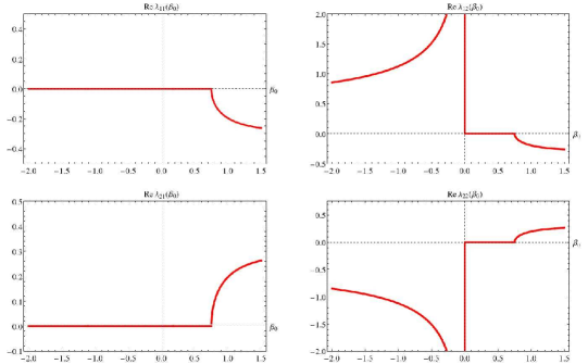
Figure 1: Plots of the real parts of the Lyapunov coefficients as a function of $\beta_{0}$.

The same conclusions can be obtained numerically. Fig. 1 shows the real part of each $\lambda_{mn}$ plotted as a function of $\beta_{0}$. The graphs show the existence of at least one eigenvalue with a positive real part when $\beta_{0}>\frac{3}{4}$ or $\beta_{0}<0$ . For $0<\beta_{0}<\frac{3}{4}$, all the eigenvalues are pure imaginary numbers.

At this point, it is interesting to recall some results presented in Ref. Berkin1990 , where the authors consider a similar higher order term in a double inflation scenario (i.e. inflation from two scalar fields). They claim that in order to have “a large range of initial conditions”,it should be $-\gamma\ll\alpha^{2}$. In our case, this condition is equivalent to impose $\beta_{0}\ll 1$. Moreover, the results above suggest that $0<\beta_{0}<\frac{3}{4}$ is a necessary condition for an inflationary scenario. The value $\frac{3}{4}$ is just an upper limit below which inflation is attainable in our model. We still have to analyze the existence of a slow-roll regime leading to a “graceful exit” (end of inflation). In what follows, we show the value $3/4$ is still an overestimated upper limit for $\beta_{0}$.

In order to illustrate how the slow-roll regime and the “graceful exit” take place in our model, we treat $X$ and $T$ as independent variables and build the direction fields numerically on the $\left(X,Y\right)$ and $\left(S,T\right)$ planes. With these assumptions,

$$\frac{\partial Y}{\partial X} =\frac{j_{1}\left(X,Y,T,S\right)}{Y},$$

$$\frac{\partial S}{\partial T} =\frac{j_{2}\left(X,Y,T,S\right)}{\beta_{0}S},$$

and we proceed with a numerical analysis summarized in Fig. 2. The direction fields on the $\left(X,Y\right)$-phase-space plane were built for fixed values of $\beta_{0}$ , $T$ and $S$. The directions fields on the $\left(T,S\right)$ plane are built for fixed values of $\beta_{0}$, $X$ and $Y$.

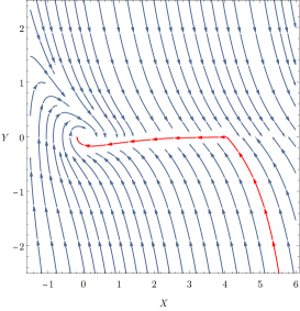
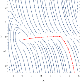
Figure 2: Plots of the direction fields on the $\left(X,Y\right)$-phase-space plane for $\beta_{0}=10^{-3}$ (left) and for $\beta_{0}=10^{-1}$ (right) with $T=1$ and $S=0.1$. The attractor line solution is present for a set of values chosen for $T$ and $S$ as large as $-100\lesssim(T,S)\lesssim+100$. Further details are given in the text.

The most important feature of the plots shown in Fig. 2 is the existence of a horizontal attractor line solution. This solution is present throughout the range $0\leq\beta_{0}<\frac{3}{4}$ for a large range of values of $T$ and $S$, typically $-100\leq\left(T,S\right)\leq 100$. A more complete graphical analysis where we vary $T$ and $S$ also shows that the horizontal attractor line shifts slightly to the right for larger values of $\left|T\right|$ and $\left|S\right|$. The direction fields on the $\left(X,Y\right)$-phase space resemble those obtained in Starobinsky model: We have an attractor region which eventually leads the trajectories to the origin of the $\left(X,Y\right)$ plane. The trajectories are slightly different from those of the Starobinky model (there are small differences on the slope of the attractor solution) but they are also characterized by positive values of $X$ and by $Y$-coordinates that are negative and small in magnitude. It is important to realize that while the trajectories on the $\left(X,Y\right)$ plane evolve in time in the direction of the point $X=Y=0$, the trajectories on the $\left(S,T\right)$ plane concomitantly evolve to $T=S=0$ (see the sequence of plots in Fig. 3).

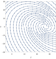
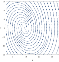
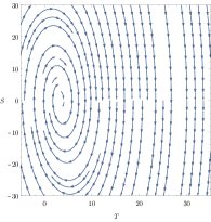
Figure 3: Plots of the direction fields on the $\left(T,S\right)$-phase-space plane for $X=4$ (left), $X=3$ (middle) and $X=2$ (right) with $\beta_{0}=10^{-2}$. The small value of $Y$ is set by Eq. (35).

In the $\left(T,S\right)$ space (Fig. 3), we do not see an attractor line region as clearly as on the $\left(X,Y\right)$ plane (Fig. 2). However, we verify the existence of an accumulation point that moves towards the origin as $X$ and $Y$ evolve on the attractor solution. Besides, this accumulation point — characterized by a constant value of $S$, namely $S\sim 0$ — is present throughout the range $0\leq\beta_{0}<\frac{3}{4}$.

Therefore, the trajectories on both $\left(X,Y\right)$ and $\left(T,S\right)$ planes allow us to identify an attractor region in a neighbourhood of which the field equations can be approximated.

III.1.2 Approximated equations in the attractor region: inflationary regime

We start by characterizing the magnitude of $\beta_{0}$ by a parameter $X^{\ast}$ such that

$$\beta_{0}\equiv e^{-X^{\ast}}<\frac{3}{4}.$$

The field equations will be analyzed in the attractor sub-region of the phase space where $X<X^{\ast}$ which implies $\beta_{0}<e^{-X}$. In addition, from the discussion around the graphic results (Figs. 2 and 3) we can assume

$$\left|Y\right|\ll 1\text{ with }Y<0,$$ (33)

and

$$S\ll T,\qquad\left|S\right|\ll 1.$$ (34)

If we recall that $\dot{S}=\frac{\partial S}{\partial X}Y$ , $\frac{\partial S}{\partial X}\ll 1$, $\frac{\partial Y}{\partial X}\ll 1$ in the attractor region, then the terms in Eqs. (27), (28) and (29) can be compared order by order. As a result, they can be approximated by

$$Y \simeq-\frac{1}{3}h_{\kappa}^{-1}\frac{e^{-X}}{\left(3-\beta_{0}e^{X}\right)},$$ (35)

$$T \simeq-Ye^{2X},$$ (36)

$$h_{\kappa}^{2} \simeq\frac{1}{12}\left(1-2e^{-X}\right).$$ (37)

With these equations, variables $Y$ and $T$ can be determined once $\beta_{0}$ and $X$ are given.

One of the most important results of these approximate solutions lies on Eq. (37): it shows the quasi-exponential behaviour of the scale factor. This expression also reveals that the greater the values of $X$ the closer the scale factor behaves to an exponential growth. Thus, we conclude that the attractor region corresponds to an inflationary expansion regime.

Several tests were performed to check the consistency of this approximation with the above numerical results. As a summary, we point out that the greater the value of $X$ (respecting $X<X^{\ast}$) the better the above equations will describe the exact results. From a practical point of view, the above expressions will already constitute an excellent approximation of the attractor phase for $X\geq 2$. For example, we obtain $T=26.2,$ $8.7$ or $3.4$ for $\beta_{0}=10^{-2}$ and $X=4,3$ or $2$ respectively, showing that the accumulation points in the plots of Fig. 3 are very well localized.

Now we are ready to evaluate the slow-roll parameters.

Slow roll parameters and number of e-folds:

In order to accommodate a slow-roll quasi-exponential inflation, any model must satisfy the following conditions:

$$\epsilon_{H} =-\frac{1}{H^{2}}\frac{dH}{dt}\ll 1,$$ (38)

$$\eta_{H} =\frac{1}{H\epsilon}\frac{d}{dt}\left(\frac{1}{H^{2}}\frac{dH}{dt}\right)\ll 1.$$ (39)

In our case, the approximations of the field equations around the slow-roll attractor lead to:

$$\epsilon_{H} \approx\frac{4e^{-2X}}{3\left(1-\frac{\beta_{0}}{3}e^{X}\right)},$$ (40)

$$\eta_{H} \approx-\frac{8}{3}\frac{\left(1-\frac{\beta_{0}}{2}e^{X}\right)}{\left(1-\frac{\beta_{0}}{3}e^{X}\right)^{2}}e^{-X}.$$ (41)

The denominator of both expressions demand that $\frac{\beta_{0}}{3}e^{X}\neq 1$. Actually, as will be seen below, the approximations demand $\frac{\beta_{0}}{3}e^{X}<1$ for consistency with condition $X<X^{\ast}$. Note that the slow-roll parameters are suppressed by $e^{-X}$ factors. This suggests sorting all quantities in orders of slow-roll according to the number of factors $e^{-X}$ they display. Thus, $\epsilon_{H}$ and $\eta_{H}$ are second- and first-order slow-roll quantities, respectively. This type of classification will be especially important in the approximation of perturbative equations.

The number of $e$-folds is now evaluated. As usual LiddleLyth , it is defined as

$$N\equiv\ln\left(\frac{a_{\text{end}}}{a}\right)=\int\limits_{t}^{t_{\text{end}}}Hdt,$$

where subscript ${}_{\text{end}}$ corresponds to the end of inflation. The attractor phase imposes a monotonic relation between $X$ and $t$ during the inflationary regime. Hence, Eq. (35) can be used to recast $N$ in the form

$$N\simeq-3\int\limits_{X}^{X_{\text{end}}}h_{\kappa}^{2}\left[\frac{3-\beta_{0}e^{X}}{e^{-X}}\right]dX$$

The upper limit of this integral is taken as $X_{\text{end}}\simeq 0$. In the slow-roll approximation, the integral gives:

$$N\simeq\frac{3}{4}e^{X}-\frac{1}{8}\beta_{0}e^{2X}.$$ (42)

This equation establishes a relation between $e^{X}$ and the number of e-folds, which can be used to write the former as function of the latter. Since this is a second order equation for $e^{X}$, two solutions are found:

$$e^{X}=\frac{3}{\beta_{0}}\left[1\pm\sqrt{1-\frac{8}{9}\beta_{0}N}\right]$$

The “$+$” sign must be discarded, should our model restore Starobinsky’s results in the limit $\beta_{0}\rightarrow 0$. That is what will be assumed henceforth:

$$e^{X}=\frac{3}{\beta_{0}}\left[1-\sqrt{1-\frac{8}{9}\beta_{0}N}\right].$$ (43)

It is clear from this expression that real values for $e^{X}$ are obtained only if $N\leq\frac{9}{8\beta_{0}}$. This fixes an upper limit for $N$ and, consequently, for $e^{X}$:

$$N_{\max}=\frac{9}{8\beta_{0}}\Rightarrow e^{X_{\max}}=\frac{3}{\beta_{0}}.$$

These values cannot be physically attained and should be considered solely as constraints, since they actually provoke the divergence of the slow-roll parameters violating the conditions for inflation. From these results, it is clear that the maximum number of e-folds and $X_{\max}$ are determined given a value for $\beta_{0}$. We will use the above results in the following way: Given physical limits for $N$, we expect to set physical limits to $\beta_{0}$. As we can see from Eq. (43),

$$e^{X}<\frac{3}{\beta_{0}}\Rightarrow\beta_{0}<\frac{9}{8N}.$$

Observationally, it is usually expected $N\geq 50$. Thus, we must have $\beta_{0}<0.0225$ for consistency.

IV Perturbed cosmological equations

An important feature of the inflationary paradigm is to engender the primordial seeds responsible for the large-scale structures formation observed in our universe. Usually, these seeds are generated from small quantum fluctuations in a homogeneous and isotropic background during the inflationary regime. Thus, in order to study the characteristics of these fluctuations in the context of our model, it is necessary to perturb the cosmological field equations obtained in Section II.

The fundamental quantities to be perturbed are:

$$\Phi =\Phi_{\left(0\right)}+\delta\Phi,$$

$$\xi^{\mu} =\xi_{\left(0\right)}^{\mu}+\delta\xi^{\mu},$$

$$g_{\mu\nu} =g_{\mu\nu\left(0\right)}+\delta g_{\mu\nu},$$

where index $\left(0\right)$ indicates a background quantity. Vector and tensor perturbations ($\delta\xi^{\mu}$ and $\delta g_{\mu\nu}$) can be decomposed into irreducible scalar-vector-tensor perturbations (SVT decomposition). Thus, using the notation defined in Eq. (22), it is possible to write the above quantities as

$$\delta\Phi =M_{Pl}\sqrt{\frac{3}{2}}\delta X,$$ (44)

$$\delta\xi^{0} =\kappa_{0}^{3/2}\delta T,$$ (45)

$$\delta\xi^{i} =\kappa_{0}^{3/2}\left(\frac{1}{\kappa_{0}^{1/2}}\left(\partial^{i}\delta W\right)+\delta V^{i}\right),$$ (46)

and

$$\delta g_{00} =-2\delta A,$$ (47)

$$\delta g_{0i} =\frac{1}{\kappa_{0}^{1/2}}\left(\partial_{i}\delta B\right)+\delta B_{i},$$ (48)

$$\delta g_{ij} =a^{2}\left[2\delta_{ij}\delta C+\frac{2}{\kappa_{0}}\left(\partial_{i}\partial_{j}\delta E\right)+\frac{1}{\kappa_{0}^{1/2}}\partial_{i}\delta E_{j}+\frac{1}{\kappa_{0}^{1/2}}\partial_{j}\delta E_{i}+2\delta E_{ij}\right],$$ (49)

where $\partial^{i}=g_{\left(0\right)}^{ij}\partial_{j}$. The $\kappa_{0}^{1/2}$ factors were included to make all perturbations dimensionless. Notice that the perturbation $\delta\xi^{\mu}$ is decomposed via SVT in two scalar degrees of freedom (namely, $\delta T$ and $\delta W$) and a vectorial one ($\delta V^{i}$). This decomposition is analogous to the one performed for $\delta g_{0\mu}$, cf. Eqs. (47) and (48).

The complete line element reads:

$$ds^{2} =-\left(1+2\delta A\right)dt^{2}+\left[\frac{2}{\kappa_{0}^{1/2}}\left(\partial_{i}\delta B\right)+2\delta B_{i}\right]dtdx^{i}$$

$$+a^{2}\left[\left(1+2\delta C\right)\delta_{ij}+\frac{2}{\kappa_{0}}\partial_{i}\partial_{j}\delta E+\frac{1}{\kappa_{0}^{1/2}}\left(\partial_{i}\delta E_{j}+\partial_{j}\delta E_{i}\right)+2\delta E_{ij}\right]dx^{i}dx^{j}.$$ (50)

Consequently, there are seven scalar perturbed quantities ($\delta X$, $\delta T$, $\delta W$, $\delta A$, $\delta B$, $\delta C$ and $\delta E$), three divergenceless vector perturbations ($\delta V^{i}$, $\delta B_{i}$ and $\delta E_{i}$) and one transverse-traceless tensor perturbation ($\delta E_{ij}$).

In addition to these eleven fundamental perturbed quantities, it is also adequate to introduce auxiliary perturbations associated with the energy-momentum tensor of an imperfect fluid — Eq. (10). In effect, we shall consider the four perturbed quantities $\delta\varepsilon$, $\delta p$, $\delta u^{\mu}$ and $\delta q_{\mu}$ coming from Eq. (10) with null viscous shear tensor. Under the constraints $u^{\mu}u_{\mu}=-1$ and $u^{\mu}q_{\mu}=0$, perturbations $\delta u^{\mu}$ and $\delta q_{\mu}$ can be decomposed as:

$$\delta u^{0} =-\delta A,$$ (51)

$$\delta u^{i} =\frac{1}{\kappa_{0}^{1/2}}\partial^{i}\delta v+\delta w^{i},$$ (52)

$$\delta q_{0} =0,$$ (53)

$$\delta q_{i} =\frac{1}{\kappa_{0}^{1/2}}\partial_{i}\delta q+\delta r_{i},$$ (54)

where $\delta w^{i}$ and $\delta r_{i}$ are vectors of zero divergence. It is noteworthy that scalar, vector and tensor perturbations evolve independently in the linear regime; therefore each set can be treated separately.

IV.1 Scalar equations

In the linear regime of perturbations there are six scalar field equations: One associated with the scalaron $\Phi$, two related to the vector field $\xi^{\mu}$ and three coming from Einstein equations.

By perturbing Eq. (8) we obtain, after an extensive manipulation, the expression

$$2\dot{Y}\delta A+Y\left(\delta\dot{A}-3\delta\dot{C}-\bar{\partial}_{0}\left(a^{2}\bar{\nabla}^{2}\delta E\right)\right)+6h_{\kappa}Y\delta A+\frac{Y}{\sqrt{3}}\bar{\nabla}^{2}\left(\delta B\right)$$

$$-3h_{\kappa}\delta\dot{X}-\delta\ddot{X}+\bar{\nabla}^{2}\left(\delta X\right)+\frac{1}{3}e^{-X}\delta X\left(1-2e^{-X}\right)$$

$$+\frac{\beta_{0}}{3}e^{-2X}f\left(\delta X,\delta T,\delta W,\delta A,\delta C,\delta E\right)=0,$$ (55)

where

$$f\left(\delta X,\delta T,\delta W,\delta A,\delta C,\delta E\right)=$$

$$= \left[e^{X}+2\beta_{0}\left(3h_{\kappa}T-2TY+S\right)\right]\left[\left(3h_{\kappa}T-2TY+S\right)\delta X+\left(2Y-3h_{\kappa}\right)\delta T+2T\delta\dot{X}\right]$$

$$-\left[e^{X}+2\beta_{0}\left(3h_{\kappa}T-2TY+S\right)\right]\left[\delta\dot{T}+\bar{\nabla}^{2}\left(\delta W\right)+T\left(\delta\dot{A}+3\delta\dot{C}+\bar{\partial}_{0}\left(a^{2}\bar{\nabla}^{2}\delta E\right)\right)\right]$$

$$-Te^{-X}\left(\frac{3}{2}T\delta X-\delta T-T\delta A\right).$$ (56)

The dimensionless barred operator is defined as:

$$\bar{\nabla}^{2}Q\equiv\frac{1}{\kappa_{0}a^{2}}\delta^{ji}\partial_{j}\partial_{i}Q.$$

Notice that only the third line in Eq. (55) corresponds to corrections to Starobinsky inflation.

The perturbed equations associated with $\xi^{0}$ and $\xi^{i}$, Eq. (7), lead to

$$\bar{\partial}_{0}\left[e^{X}\delta X+\beta_{0}\left[\left(3h_{\kappa}-2Y\right)\delta T+\delta\dot{T}-2T\delta\dot{X}+\bar{\nabla}^{2}\left(\delta W\right)+T\left(\delta\dot{A}+3\delta\dot{C}+\bar{\partial}_{0}\left(a^{2}\bar{\nabla}^{2}\delta E\right)\right)\right]\right]$$

$$-e^{-X}\left(T\delta X-2T\delta A-\delta T\right)=0$$ (57)

and

$$\partial_{j}\left[e^{X}\delta X+\beta_{0}\left[\left(3h_{\kappa}-2Y\right)\delta T+\delta\dot{T}-2T\delta\dot{X}+\bar{\nabla}^{2}\left(\delta W\right)+T\left(\delta\dot{A}+3\delta\dot{C}+\bar{\partial}_{0}\left(a^{2}\bar{\nabla}^{2}\delta E\right)\right)\right]\right]$$

$$-e^{-X}\partial_{j}\left[\left(T\delta B+\delta W\right)\right]=0.$$ (58)

By combining these two equations we can obtain a simpler expression, given by

$$\partial_{j}\left[T\delta X-\delta T+Y\delta W-\delta\dot{W}-2T\delta A+YT\delta B-S\delta B-T\delta\dot{B}\right]=0.$$ (59)

It is also necessary to perturb Einstein equations. These equations, in a gauge invariant form Mukhanov , are given by

$$\bar{\nabla}^{2}\Psi-3h_{\kappa}\left(\dot{\Psi}+h_{\kappa}\Psi\right) =-\frac{\widetilde{\delta\varepsilon}}{2\kappa_{0}M_{Pl}^{2}},$$ (60)

$$\dot{\Psi}+h_{\kappa}\Psi =\frac{1}{2\kappa_{0}M_{Pl}^{2}}\left[\left(\varepsilon+p\right)\widetilde{\delta v}+\widetilde{\delta q}\right],$$ (61)

$$\ddot{\Psi}+4h_{\kappa}\dot{\Psi}+\left(2\dot{h}_{\kappa}+3h_{\kappa}^{2}\right)\Psi =-\frac{\widetilde{\delta p}}{2\kappa_{0}M_{Pl}^{2}},$$ (62)

where the choice of different gauges can be made through the expressions:

$$\Psi =-\delta A-\bar{\partial}_{0}\left(\delta B-a^{2}\delta\dot{E}\right),$$ (63)

$$\widetilde{\delta\varepsilon} =\delta\varepsilon+\dot{\varepsilon}_{\left(0\right)}\left(\delta B-a^{2}\delta\dot{E}\right),$$ (64)

$$\widetilde{\delta p} =\delta p+\dot{p}_{\left(0\right)}\left(\delta B-a^{2}\delta\dot{E}\right),$$ (65)

$$\widetilde{\delta v} =\delta v+a^{2}\delta\dot{E},$$ (66)

$$\widetilde{\delta q} =\delta q.$$ (67)

The last equation states that the heat flux $\delta q$ is naturally gauge invariant. In addition to Eqs. (60), (61) and (62), we have the constraint

$$\delta A+\delta C=-\frac{1}{a}\bar{\partial}_{0}\left[a\left(\delta B-a^{2}\delta\dot{E}\right)\right],$$ (68)

arising from Einstein’s equation $\delta G_{ij}=M_{Pl}^{-2}\delta T_{ij}$ with $i\neq j$. The relationship between the quantities $\delta\varepsilon$, $\delta p$, $\delta v$ and $\delta q$ and the fundamental scalar perturbations are obtained from the Eqs. (11), (12) and (13). By perturbing these equations we obtain

$$\delta\varepsilon+\delta p =3\kappa_{0}M_{Pl}^{2}\left[Y\delta\dot{X}-Y^{2}\delta A+\frac{\beta_{0}}{3}e^{-3X}T\left(\frac{3}{2}T\delta X-\delta T-T\delta A\right)\right],$$ (69)

$$\delta v =-\frac{\delta X+Y\delta B+\sqrt{\frac{\beta_{0}e^{-3X}}{3}}\delta W}{\left(Y-\sqrt{\frac{\beta_{0}e^{-3X}}{3}}T\right)},$$ (70)

$$\delta q =\frac{3}{2}\sqrt{\frac{\beta_{0}e^{-3X}}{3}}\kappa_{0}M_{Pl}^{2}\left(T\delta X+YT\delta B+Y\delta W\right).$$ (71)

These last three equations together with the perturbation for $\delta\varepsilon$ — see Appendix A — complete the description of the perturbed Einstein’s equations.

The set of equations (55, 57, 58, 60, 61, 62, 68) establishes the dynamics of the scalar perturbations. Let us emphasize that not all of these perturbations are dynamical quantities. Actually, a quick analyzis of the Cauchy problem shows that only four of these equations are truly dynamical equations, while three of them constitute constraints between the variables. It is interesting to note that the number of degrees of freedom in our higher-order scalar-vector approach is in agreement with the number of degrees of freedom in the higher-order two-scalar approach of Ref. Castellanos2018 . In the later case, besides the perturbations of the two scalar fields, there are two scalar perturbations from the metric.

Here, two of the seven scalar perturbations can be “eliminated" by an appropriate gauge choice. Moreover, Eq. (68) allows us to write either $\delta C$ or $\delta A$ in terms of the other three metric perturbations. Thus, the problem is completely characterized by four differential equations. Since the expressions for $\delta\varepsilon$ and $\delta p$ contain a lot of terms, it is convenient to select a set of equations avoiding these perturbations. A natural choice here is to work with Eqs. (55), (58), (59) and (61). This will be done in Section V.1 with the use of slow-roll approximation.

IV.2 Vector and tensor equations

There are three fundamental equations associated with vector perturbations. The first one is obtained by perturbing Eq. (7); the result is:

$$\delta V_{i}=-T\delta B_{i}.$$ (72)

The other two come from perturbations in $0i$- and $ij$-components of Einstein’s equations:

$$\bar{\nabla}^{2}\delta F_{i} =\frac{2}{a\kappa_{0}M_{Pl}^{2}}\left[\left(\varepsilon+p\right)\widetilde{\delta w_{i}}+\widetilde{\delta r_{i}}\right],$$ (73)

$$\partial_{i}\delta\dot{F}_{j}+\partial_{j}\delta\dot{F}_{i}+h_{\kappa}\left(\partial_{i}\delta F_{j}+\partial_{j}\delta F_{i}\right) =0,$$ (74)

where

$$\delta F_{i} =\delta B_{i}-a^{2}\delta\dot{E}_{i},$$ (75)

$$\widetilde{\delta w_{i}} =\delta w_{i}+\delta B_{i},$$ (76)

$$\widetilde{\delta r_{i}} =\delta r_{i},$$ (77)

are gauge invariant quantities. Due to the constraint (72), it is possible to show that

$$\widetilde{\delta w_{i}}=\widetilde{\delta r_{i}}=0,$$ (78)

i.e. the effective energy-momentum tensor (9) has no vector perturbations. This result was expected since the term $\nabla_{\mu}R\nabla^{\mu}R$ responsible for the extra vector perturbations can be written as $-R\square R$, which contains only scalar degrees of freedom (see Wands1994 ).

Finally, there is only one equation associated with the tensor degree of freedom:

$$\delta\ddot{E}_{ij}+3h_{\kappa}\delta\dot{E}_{ij}-\bar{\nabla}^{2}\delta E_{ij}=0.$$ (79)

This equation is derived from $\delta G_{ij}=M_{Pl}^{-2}\delta T_{ij}$ and represents gravitational waves freely propagating in a homogeneous and isotropic background.

V Solutions of the perturbed cosmological equations

The equations derived in the previous section are complicated. However, in the attractor region, where the slow-roll approximation is valid, these equations are considerably simplified and they can be treated analytically.

V.1 Scalar solutions

The implementation of approximations in the scalar equations should take into account that, in general, different perturbations in a given gauge have different orders of slow-roll. For example, in the Newtonian gauge, Eq. (61) for Starobinsky inflation ($\beta_{0}=0$) is written as

$$\delta\dot{A}+h_{\kappa}\delta A=\frac{3}{4}Y\delta X.$$

During the inflationary regime, where $h_{\kappa}\sim 1$, this equation tells us $\delta A\sim Y\delta X\sim e^{-X}\delta X$, which means that the metric perturbation is a slow-roll factor smaller than the scalar field perturbation.

For the case $\beta_{0}\neq 0$, the situation is more complicated because Eqs. (58) and (59) indicate that the perturbations $\delta T$ and $\delta W$ are different from $\delta X$ concerning the order of slow-roll factors. This can be explicitly seen by writing Eq. (58) in the Newtonian gauge

$$e^{X}\delta X+\beta_{0}\left[\left(3h_{\kappa}-2Y\right)\delta T+\delta\dot{T}-2T\delta\dot{X}+\bar{\nabla}^{2}\left(\delta W\right)-2T\delta\dot{A}\right]-e^{-X}\left(\delta W\right)=0.$$ (80)

As in the attractor sub-region $\beta_{0}\lesssim e^{-X}$ and $T\sim e^{X}$ (see Section III.1.2), this equation tells us that $\delta T$ or $\delta W$ must be two slow-roll factors larger than $\delta X$. Moreover, Eq. (59)

$$T\delta X-\delta T+Y\delta W-\delta\dot{W}-2T\delta A=0$$ (81)

shows that $\delta T$ and $\delta W$ are of the same order in slow-roll. Thus, in the Newtonian gauge, Eqs. (80), (81) and (61) suggest that

$$\delta T \sim\delta W\sim e^{2X}\delta X,$$ (82)

$$\delta A \sim e^{-X}\delta X.$$ (83)

The next step is to use (82) and (83) to simplify the expressions (55), (58) and (59). During the inflationary regime:

$$T\sim e^{X}\text{, }Y\sim e^{-X}\text{, }h_{\kappa}\sim 1\text{\ e }\beta_{0}\lesssim e^{-X}\text{\ .}$$

So, up to slow-roll leading order, Eqs. (55), (58) and (59) are approximated by:

$$\delta\ddot{X}+3h_{\kappa}\delta\dot{X}-\bar{\nabla}^{2}\left(\delta X\right)+\frac{\beta_{0}}{3}e^{-X}\left[3h_{\kappa}\delta T+\delta\dot{T}+\bar{\nabla}^{2}\left(\delta W\right)\right] \simeq 0,$$ (84)

$$\delta X-e^{-2X}\delta W+\beta_{0}e^{-X}\left[3h_{\kappa}\delta T+\delta\dot{T}+\bar{\nabla}^{2}\left(\delta W\right)\right] \simeq 0,$$ (85)

$$\delta\dot{W}+\delta T \simeq 0.$$ (86)

In the Starobinsky limit Eqs. (85) and (86) are not present and Eq. (84) reduces to the usual expression for a single scalar field. The combination of the three previous equations results in

$$\delta\ddot{X}+3h_{\kappa}\delta\dot{X}-\bar{\nabla}^{2}\left(\delta X\right) \simeq\frac{1}{3}\left(\delta X-e^{-2X}\delta W\right),$$ (87)

$$\beta_{0}e^{-X}\left[\delta\ddot{W}+3h_{\kappa}\delta\dot{W}-\bar{\nabla}^{2}\left(\delta W\right)\right] \simeq\delta X-e^{-2X}\delta W.$$ (88)

In the slow-roll leading-order approximation, background terms can be considered constant with respect to time derivatives, i.e.

$$\bar{\partial}_{0}\left(e^{-X}\delta W\right)=\delta W\bar{\partial}_{0}\left(e^{-X}\right)+e^{-X}\bar{\partial}_{0}\left(\delta W\right)\simeq e^{-X}\bar{\partial}_{0}\left(\delta W\right).$$

Let

$$\delta\varphi_{1}\equiv a\delta X\text{ e }\delta\varphi_{2}\equiv ae^{-2X}\delta W$$

Eqs. (87) and (88) then turn to

$$\delta\varphi_{1}^{\prime\prime}+\left(k^{2}-\frac{a^{\prime\prime}}{a}\right)\delta\varphi_{1} \simeq\frac{\kappa_{0}a^{2}}{3}\left(\delta\varphi_{1}-\delta\varphi_{2}\right),$$ (89)

$$\beta_{0}e^{X}\left[\delta\varphi_{2}^{\prime\prime}+\left(k^{2}-\frac{a^{\prime\prime}}{a}\right)\delta\varphi_{2}\right] \simeq\kappa_{0}a^{2}\left(\delta\varphi_{1}-\delta\varphi_{2}\right),$$ (90)

where prime (^′) indicates derivative with respect to the conformal time $\eta$. Notice that by introducing the factor $e^{-2X}$ in the definition of $\delta\varphi_{2}$ we assure $\delta\varphi_{1}$ and $\delta\varphi_{2}$ are of the same slow-roll order. Moreover, a (quasi-)de Sitter spacetime satisfies $12H^{2}\simeq\kappa_{0}$; then,

$$a\simeq-\frac{1}{H\eta}\Rightarrow\frac{a^{\prime\prime}}{a}\simeq 2a^{2}H^{2}\simeq\frac{2}{\eta^{2}}.$$

and Eqs. (89) and (90) lead to

$$\delta\varphi_{1}^{\prime\prime}+k^{2}\left(1-\frac{2}{\eta^{2}k^{2}}\right)\delta\varphi_{1} \simeq\frac{4}{k^{2}\eta^{2}}k^{2}\left(\delta\varphi_{1}-\delta\varphi_{2}\right),$$ (91)

$$\beta_{0}e^{X}\left[\delta\varphi_{2}^{\prime\prime}+k^{2}\left(1-\frac{2}{\eta^{2}k^{2}}\right)\delta\varphi_{2}\right] \simeq\frac{12}{k^{2}\eta^{2}}k^{2}\left(\delta\varphi_{1}-\delta\varphi_{2}\right).$$ (92)

The solution to the above pair of equations depends on initial conditions deep in the sub-horizon regime, i.e. for $k\eta\gg 1$. In this case,

$$\delta\varphi_{1,2}^{\prime\prime}+k^{2}\delta\varphi_{1,2}\simeq 0,\qquad k\eta\gg 1,$$

and the initial conditions $\left(\delta\varphi_{1i},\delta\varphi_{2i}\right)$ are the same because they come from the quantization of identical equations. Condition $\delta\varphi_{1i}=\delta\varphi_{2i}$ causes the vanishing of the right-hand side of Eqs. (91) and (92) for all $\eta$. For this reason, the evolution of $\left(\delta\varphi_{1},\delta\varphi_{2}\right)$ is dictated by Mukhanov-Sasaki equation

$$\delta\varphi_{1,2}^{\prime\prime}+k^{2}\left(1-\frac{2}{\eta^{2}k^{2}}\right)\delta\varphi_{1,2}\simeq 0.$$

Therefore, we get a tracking solution:

$$\delta\varphi_{1}=\delta\varphi_{2}\Rightarrow\delta X\simeq e^{-2X}\delta W.$$ (93)

Few remarks are in order. First, the tracking solution corresponds to an adiabatic solution. In fact, the heat flux $\delta q$ vanishes in slow-roll leading order once Eq. (71) in Newtonian gauge reads:

$$\delta q\simeq\frac{3M_{Pl}^{2}\kappa_{0}}{2}\sqrt{\frac{\beta_{0}e^{X}}{3}}Y\left(e^{-2X}\delta W-\delta X\right)\simeq 0.$$

This is the reason for the comoving curvature being conserved at super-horizon scales (cf. Appendix B).

A second remark is: The tracking solution follows the attractor trajectory defined by the background fields in the phase space. This is checked by taking the time derivative of (93)

$$\delta\dot{W}\simeq e^{2X}\delta\dot{X}$$

and using Eqs. (22) and (86). Then,

$$\delta T\simeq-e^{2X}\delta Y,$$

which is of the same type as (36). The fact that the tracking solution follows the attractor line is not so surprising because the multi-field adiabatic perturbations in inflationary models are defined as the ones remaining along the background trajectory of the homogeneous and isotropic fields Wand2008 .

Finally, something should be said about what happens to the solutions of Eqs. (91) and (92) in the case where the initial conditions $\delta\varphi_{1i}$ and $\delta\varphi_{2i}$ are different. In order to perform this analysis, it is convenient to cast (91) and (92) in terms of the reset scale factor such that a given scale crosses the horizon $a=1$, i.e. $k=H$. In this case,

$$\delta\varphi_{1}^{\ast\ast}+\frac{2}{a}\delta\varphi_{1}^{\ast}+\left(\frac{1}{a^{4}}-\frac{2}{a^{2}}\right)\delta\varphi_{1} \simeq\frac{4}{a^{2}}\left(\delta\varphi_{1}-\delta\varphi_{2}\right),$$ (94)

$$\beta_{0}e^{X}\left[\delta\varphi_{2}^{\ast\ast}+\frac{2}{a}\delta\varphi_{2}^{\ast}+\left(\frac{1}{a^{4}}-\frac{2}{a^{2}}\right)\delta\varphi_{2}\right] \simeq\frac{12}{a^{2}}\left(\delta\varphi_{1}-\delta\varphi_{2}\right),$$ (95)

where * denotes differentiation with respect to the scale factor and $\beta_{0}e^{X}$ is given by (43). Eqs. (94) and (95) can be studied for different sets of initial conditions $\left\{\delta\varphi_{1i}\text{;}\delta\varphi_{2i}\right\}$ and $\left\{\delta^{\ast}\varphi_{1i}\text{;}\delta^{\ast}\varphi_{2i}\right\}$ assuming that $k$ crosses the horizon in the interval $50\leq N\leq 60$. A numerical procedure showed the differences between $\delta\varphi_{1}$ and $\delta\varphi_{2}$ are never amplified; furthermore, they are suppressed by the expansion in the super-horizon regime ($a>1$). We conclude that any eventual non-adiabatic perturbation generated by higher-order corrections may be neglected in slow-roll leading order.

In view of the considerations above, we state that perturbations $\delta X$ and $\delta W$ have the same dynamics in first order in slow-roll, both being described by Mukhanov-Sasaki-type equations

$$\delta\ddot{X}+3h_{\kappa}\delta\dot{X}-\bar{\nabla}^{2}\left(\delta X\right) \simeq 0,$$ (96)

$$\delta\ddot{W}+3h_{\kappa}\delta\dot{W}-\bar{\nabla}^{2}\left(\delta W\right) \simeq 0.$$ (97)

It is now necessary to decide on which variable is to be quantized. This variable is associated to the comoving curvature perturbation

$$\mathcal{R}\equiv\delta C+h_{\kappa}\left(\delta v+\delta B\right)$$ (98)

which in Newtonian gauge is reduced to

$$\mathcal{R}=-\delta A+h_{\kappa}\delta v$$ (99)

where

$$\delta v=-\frac{\delta Q}{Y-\sqrt{\frac{\beta_{0}e^{-3X}}{3}}T}$$

with

$$\delta Q\equiv\delta X+\sqrt{\frac{\beta_{0}e^{-3X}}{3}}\delta W.$$ (100)

In slow-roll leading order, $\delta A$ can be neglected in (99) and the curvature perturbation is approximated by

$$\mathcal{R\simeq}-\frac{h_{\kappa}}{Y\left(1+\sqrt{\frac{\beta_{0}e^{X}}{3}}\right)}\delta Q,$$ (101)

where $\delta Q$ is the generalization of Mukhanov-Sasaki variable. In addition, the denominator of Eq. (101) represents the normalization of $\delta v$ given by Eq. (16). It is important to stress that $\mathcal{R}$ is a gauge invariant quantity which is conserved in super-horizon scales (see Appendix B). We also note that the normalization of ${\cal R}$ in Eq. (101) is analogous to the two-field inflation case Wand2008 ; the difference being the non-canonical kinetic factor $\beta_{0}e^{X}/3$ associated to the perturbation $e^{-2X}\delta W$ — see Eqs. (89) and (90).

A convenient combination of Eqs. (96) and (97) leads to:

$$\delta\ddot{Q}+3h_{\kappa}\delta\dot{Q}-\bar{\nabla}^{2}\left(\delta Q\right)\simeq 0.$$ (102)

By defining

$$\delta\varphi\equiv aM_{Pl}\sqrt{\frac{3}{2}}\delta Q,$$

it is possible to write Eq. (102) in Fourier space as

$$\delta\varphi_{{}_{\vec{k}}}^{\prime\prime}+\left(k^{2}-\frac{a^{\prime\prime}}{a}\right)\delta\varphi_{{}_{\vec{k}}}\simeq 0.$$ (103)

This is the usual Mukhanov-Sasaki equation which can be quantized in the standard way MuFeBran ; BaumannLectures . Thereby, the dimensionless power spectrum $\Delta_{\delta Q}^{2}$ related to $\delta Q$ perturbation is given by

$$\Delta_{\delta Q}^{2}\simeq\frac{2}{3M_{Pl}^{2}}\left.\left(\frac{H}{2\pi}\right)^{2}\right|_{k=Ha}.$$ (104)

The index $k=Ha$ indicates the power spectrum is calculated at the specific time the perturbation crosses the horizon.

In order to compare the theoretical result with observations, it is necessary to rewrite the power spectrum in terms of the curvature perturbation. From Eqs. (40), (101) and (104), we obtain

$$\Delta_{\mathcal{R}}^{2}\simeq\frac{1}{8\pi^{2}M_{Pl}^{2}}\left.\frac{H^{2}}{\epsilon_{H}}\frac{\left(1-\sqrt{\frac{\beta_{0}e^{X}}{3}}\right)}{\left(1+\sqrt{\frac{\beta_{0}e^{X}}{3}}\right)}\right|_{k=Ha}.$$ (105)

This expression gives the curvature power spectrum in leading order for the proposed inflationary model. The extra term with respect to Starobinsky’s action produces corrections in $\Delta_{\mathcal{R}}^{2}$ coming from both background dynamics (via the generalization of $\epsilon_{H}$) and perturbations (through the generalization of $\mathcal{R}$). In the next section, we will see how this extra term affects the predictions of Starobinsky’s inflation.

V.2 Vector and tensor solutions

During the inflationary regime, vector perturbations are described by Eqs. (72), (73) and (74). By acting the operator $\delta^{jl}\partial_{l}$ onto (74) then taking the Fourier transform, we obtain

$$-k^{2}\left(\delta\dot{F}_{i\left(\vec{k}\right)}+h_{\kappa}\delta F_{i\left(\vec{k}\right)}\right)=0,$$

whose solution is

$$\delta F_{i\left(\vec{k}\right)}=\frac{C_{i\left(\vec{k}\right)}}{a}.$$

This shows $\delta F_{i}$ decays with $a\sim e^{Ht}$. As the other two vector perturbations are identically null, Eq. (78), we conclude that the proposed model does not generate any kind of vector perturbation.

The expression (79) associated to the tensor perturbation $\delta E_{ij}$ is analogous to Eq. (102). Decomposing $\delta E_{ij}$ as

$$\delta E_{ij}=\frac{\delta v}{a}e_{ij},$$

where $e_{ij}$ is the polarization tensor, and writing Eq. (79) in Fourier space, results in:

$$\delta v_{{}_{\vec{k}}}^{\prime\prime}+\left(k^{2}-\frac{a^{\prime\prime}}{a}\right)\delta v_{{}_{\vec{k}}}=0.$$ (106)

This is the standard Mukhanov-Sasaki equation for tensor perturbations. Following an analogous approach to the scalar case LiddleLyth ; MuFeBran , one gets the tensor power spectrum:

$$\Delta_{\delta E_{ij}}^{2}\left(k\right)=\frac{8}{M_{Pl}^{2}}\left.\left(\frac{H}{2\pi}\right)^{2}\right|_{k=Ha}.$$ (107)

It is worth mentioning $\delta E_{ij}$ is a gauge invariant quantity which is conserved on super-horizon scales.

VI Constraining the cosmological parameters

The conservation of $\mathcal{R}$ and $\delta E_{ij}$ in super-horizon scales allows to directly compare the inflationary power spectra Eqs. (105) and (107) with those used as initial conditions in the description of CMB anisotropies. This comparison is made through the parameterizations

$$\Delta_{\mathcal{R}}^{2}\left(k\right) =A_{s}\left(\frac{k}{k_{\ast}}\right)^{n_{s}-1},$$ (108)

$$\Delta_{h}^{2}\left(k\right) =A_{t}\left(\frac{k}{k_{\ast}}\right)^{n_{t}},$$ (109)

where $A_{s}$ and $A_{t}$ are the scalar and tensor amplitudes, $k_{\ast}$ is the pivot scale and $n_{s}$ and $n_{t}$ are the scalar and tensor tilts Planck2018 .

By comparing Eqs. (105) and (107) to Eqs. (108) and (109) and using the slow-roll parameters $\epsilon_{H}$ and $\eta_{H}$ given in Eqs. (40) and (41), we obtain:

$$n_{s}\approx 1+\eta_{H}-2\epsilon_{H}+\frac{4}{3}\frac{\sqrt{\frac{\beta_{0}e^{-X_{\ast}}}{3}}}{\left(1-\frac{\beta_{0}e^{X_{\ast}}}{3}\right)^{2}}$$ (110)

and

$$r\equiv\frac{A_{t}}{A_{s}}\approx 16\epsilon_{H}\frac{\left(1+\sqrt{\frac{\beta_{0}e^{X_{\ast}}}{3}}\right)}{\left(1-\sqrt{\frac{\beta_{0}e^{X_{\ast}}}{3}}\right)}.$$ (111)

In addition to $n_{s}$ and $r$, there is also

$$n_{t}\approx-2\epsilon_{H}\approx-\frac{r}{8}\frac{\left(1-\sqrt{\frac{\beta_{0}e^{X_{\ast}}}{3}}\right)}{\left(1+\sqrt{\frac{\beta_{0}e^{X_{\ast}}}{3}}\right)}.$$ (112)

This expression shows how the consistency relation $n_{t}=-r/8$ LiddleLyth associated to a single scalar field inflation changes with the introduction of the higher order term in Starobinsky action.

Eqs. (110) and (111) can be written in terms of the $e$-folds number $N$, given by Eq. (43). Thus,

$$n_{s}\approx 1+\frac{4\beta_{0}}{9}\frac{\left[1-3\sqrt{1-\frac{8}{9}\beta_{0}N_{\ast}}+\sqrt{1-\sqrt{1-\frac{8}{9}\beta_{0}N_{\ast}}}\right]}{\left(1-\sqrt{1-\frac{8}{9}\beta_{0}N_{\ast}}\right)\left(1-\frac{8}{9}\beta_{0}N_{\ast}\right)}$$ (113)

and

$$r=\frac{32}{27}\frac{\beta_{0}^{2}}{\left(1-\sqrt{1-\frac{8}{9}\beta_{0}N_{\ast}}-\frac{4}{9}\beta_{0}N_{\ast}\right)\left(1-\sqrt{1-\sqrt{1-\frac{8}{9}\beta_{0}N_{\ast}}}\right)^{2}}$$ (114)

The results typical of Starobinsky inflation are recovered in the limit $\beta_{0}\rightarrow 0$:

$$\lim_{\beta_{0}\rightarrow 0}n_{s}\approx 1-\frac{2}{N_{\ast}}\text{ \ and \ }\lim_{\beta_{0}\rightarrow 0}r\approx\frac{12}{N_{\ast}^{2}}\text{.}$$

Fig. 4 displays the parametric plot $n_{s}\times r$ accounting for the model with $\beta_{0}\neq 0$ and $50\leqslant N\leqslant 60$.

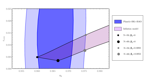
Figure 4: The blue contours correspond to $68\%$ and $95\%$ CL constraints on $n_{s}\times r$ given by Planck plus BICEP2/Keck plus BAO data BK2018 . The black circles represent Starobinsky model ($\beta_{0}=0$). As $\beta_{0}$ increases the curves move to the right (light purple region) increasing the tensor-to-scalar ratio and the scalar tilt values. The grey circles represent the upper limits for $\beta_{0}$ associated with $95\%$ CL for $n_{s}$. In this case, $N_{\ast}=50$ corresponds to $\beta_{0}=9.3\times 10^{-3}$ and $r=0.014$; and $N_{\ast}=60$ corresponds to $\beta_{0}=5.2\times 10^{-3}$ and $r=0.0076$.

Fig. 4 shows how the addition of the term $\nabla^{\mu}R\nabla_{\mu}R$ in Starobinsky action increases the spectral index value and the tensor-to-scalar ratio. The constraint of $95\%$ CL in $n_{s}$ sets upper limits of $\beta_{0}=9.3\times 10^{-3}$ and $\beta_{0}=5.2\times 10^{-3}$ for $N_{\ast}=50$ and $N_{\ast}=60$, respectively. Thus, within the observational limits, the proposed model is able to produce an increase of up to $2.9$ times in the ratio $r$ when compared to Starobinsky inflation. Furthermore, the value of $\beta_{0}\lesssim 10^{-2}\ll 1$ is consistent with the slow-roll approximation performed above. It also guarantees a large range of initial conditions able to trigger the inflationary regime (see Section III.1.1).

The energy density scale characteristic of inflation is determined by $\varepsilon\approx\left(\kappa_{0}/4\right)M_{Pl}^{2}.$ From Eqs. (105) and (108) in combination with Eq. (114), we obtain

$$\varepsilon\approx\frac{3\pi^{2}A_{s}}{2}rM_{Pl}^{4}\text{.}$$

Moreover, we see in Fig. 4 that the tensor-to-scalar ratio varies from $0.0033\leq r\leq 0.014$ within the range of $95\%$ CL. Thus, for $A_{s}\simeq 1.96\times 10^{-9}$ Planck2018 , the energy density is in the range

$$0.96\times 10^{-10}\leq\frac{\varepsilon}{M_{Pl}^{4}}\leq 4.06\times 10^{-10},$$

which is completely consistent with a sub-Planckian region.

VII Discussion

In this work, we have studied the effects of a modification to Starobinsky inflation model produced by the addition of the higher-order term $\frac{\beta_{0}}{2\kappa_{0}^{2}}\nabla_{\mu}R\nabla^{\mu}R$. We started from the generalized Starobinsky action in Einstein frame, in which the Lagrangian depends on a scalar field $\Phi$ and an auxiliary vector field $\xi^{\mu}$. We have constructed the cosmological background dynamics and the perturbative structure of the theory for this model.

The background dynamics was determined from Friedmann equations as well as from those for the auxiliary fields. After some manipulations, we have shown the existence of an attractor region in the 4-dimensional phase space ($\Phi,\dot{\Phi},\xi^{0},\dot{\xi}^{0}$) within $0<\beta_{0}<3/4$. This attractor region is consistent with a slow-roll inflationary period. In addition, we have seen that inflation ends with an oscillation of the scalar field about the origin and with $\xi^{0}\rightarrow 0$. This characterizes an usual reheating phase.

The study of the perturbative regime was performed via the SVT decomposition, as usual. We have shown that the vector and tensor degrees of freedom behave just like in Starobinsky inflation. Also, we verified that the curvature perturbation $\mathcal{R}$ (obtained from a proper combination of the scalar degrees of freedom) satisfies Mukhanov-Sasaki equation in the slow-roll leading order approximation. At last, we obtained the tensorial and curvature power spectra and compared them with the most recent observations from Keck Array and BICEP2 collaborations BK2018 .

The main results from this work are summarized in Fig. 4 and indicate how the extra term $\frac{\beta_{0}}{2\kappa_{0}^{2}}\nabla_{\mu}R\nabla^{\mu}R$ changes the observable parameters of the primordial power spectrum. In Fig. 4 we see that the parameter $\beta_{0}$ has to be less than $10^{-2}$ for a number of e-folds in the interval $50\leq N_{\ast}\leq 60$. In this case, the scalar-to-tensor rate $r$ can be expected to be up to three times the values predicted by Starobinsky model. This result is particularly interesting since it enables this natural generalization of Starobinsky model to have an $r$ up to $\sim 0.01$. Besides, the small values of $\beta_{0}$ preserves the chaotic structure of the theory, making room for a large range of consistent initial conditions Berkin1990 .

The comparison of the results obtained here with those of Ref. Castellanos2018 shows some interesting aspects. Firstly, it is important to realize that our parameter $\beta_{0}$ is mapped on $-3k$ in Ref. Castellanos2018 . Hence, the results obtained here for $\beta_{0}>0$ have to be compared to those obtained with $\gamma<0$ in Ref. Castellanos2018 . When comparing Fig. 4 of our paper with Fig. 4 in Ref. Castellanos2018 , we observe that for very low values of $\beta_{0}$ and $\gamma$ (red region in Ref. Castellanos2018 ) the models shade the same area. However, as these parameters are slightly increased, discrepancies appear. We note that our model predicts higher values for $r$ — in a rough estimate, our values are about 3 times greater than those of Ref. Castellanos2018 . Moreover, we realize that the values of $-3k$ are at least three times greater than the equivalent values of our $\beta_{0}$, when comparing the 68% CL values for $\beta_{0}$ with the minimum values of $-3k$. These differences may be due to the fact that the authors of Ref. Castellanos2018 treated the higher order term as a small perturbation of the Starobinsky model. This deserves a future and careful analyzis.

It must be highlighted that the action (3) presents ghosts for $\beta_{0}>0$ Hindawi1996 . On the other hand, the quantization procedure performed in Section V.1 does not show any pathology. The crucial point in this discussion is that scalar perturbations in slow-roll leading order become constrained by Eq. (93). Hence, there is only one degree of freedom to be quantized. This degree of freedom is the (gauge invariant) curvature perturbation, which is given by $\mathcal{R}\propto\delta Q=\delta X+\sqrt{\beta_{0}e^{-3X}/3}\delta W$ in the Newtonian gauge. Since the two terms composing $\delta Q$ have the same sign, we notice that $\delta Q$ is always a no-ghost variable. As a consequence, it can be quantized as usual, independently of the $\beta_{0}$ values. This situation is analogous to the treatment given to ghosts by effective theories. Indeed, the energy scale remains mostly unchanged during the quasi-exponential expansion (a fact that is consistent with the slow-roll approximation) and the ghost degree of freedom remains frozen.

The end of Section VI shows that the energy scale of the inflationary regime is sub-Planckian. This is a first indication that the semi-classical approach adopted here is valid. The next step is to check the naturalness, i.e. if the quantum corrections remain small in this energy scale. This was addressed in Hertzberger2010 for Starobinsky action and, since $\beta_{0}<10^{-2}$, the result should apply to our model as well. This subject shall be studied in a future work, where the $\beta_{0}$ interval compatible with the requirement for naturalness will be determined.

The higher-order modified Starobinsky inflation model presented here can be further generalized to include the spin-$2$ terms $R_{\mu\nu}R^{\mu\nu}$ and $\nabla_{\mu}R_{\alpha\beta}\nabla^{\mu}R^{\alpha\beta}$ appearing in action (2). The effects upon inflation coming from all these terms will be addressed by the authors in the future.

Appendix A Perturbation of $\delta\varepsilon$

The quantity $\delta\varepsilon$ is obtained by perturbing Eq. (14) and combining the result with Eq. (69). After a long manipulation making use of the definitions (23) and (24), we obtain:

$$\frac{2}{M_{Pl}^{2}\kappa_{0}}\delta\varepsilon =-3Y^{2}\delta A+3Y\delta\dot{X}+e^{-X}\left(1-e^{-X}\right)\delta X$$

$$+\beta_{0}e^{-X}\left(1-e^{-X}\right)\left[\delta\dot{T}+3h_{\kappa}\delta T-2Y\delta T-2T\delta\dot{X}\right]$$

$$+\beta_{0}e^{-X}\left[\left(3h_{\kappa}T-2YT+S\right)\left(e^{-X}\delta F+2e^{-X}\left(1-e^{X}\right)\delta X\right)\right]$$

$$-\beta_{0}^{2}e^{-2X}\left[\left(3h_{\kappa}T-2YT+S\right)\left[\left(3h_{\kappa}T-2YT+S\right)\delta X+T\left(\delta\dot{A}+\delta\dot{D}\right)+\bar{\nabla}^{2}\delta W\right]\right]$$

$$+\beta_{0}e^{-2X}\left[\left(2YF-\dot{F}-3h_{\kappa}F\right)\delta T-F\delta\dot{T}+\left(2YT-3h_{\kappa}T-S\right)\delta F-T\delta\dot{F}\right]$$

$$+2\beta_{0}e^{-2X}\left[\left(SF+T\dot{F}-2YTF+3h_{\kappa}TF\right)\delta X+2TF\delta\dot{X}\right]$$

$$+3\beta_{0}e^{-3X}T\left[\frac{3}{2}T\delta X-\delta T-T\delta A\right],$$ (115)

where

$$F =e^{X}-1+\beta_{0}\left(3h_{\kappa}T-2YT+S\right),$$

$$\delta F =e^{X}\delta X+\beta_{0}\left[T\delta\dot{D}+\delta\dot{T}+3h_{\kappa}\delta T+\bar{\nabla}^{2}\delta W-2Y\delta T-2T\delta\dot{X}\right],$$

and

$$\delta D=-\frac{\delta g}{2a^{6}}=\delta A+3\delta C+a^{2}\bar{\nabla}^{2}\delta E,$$

where $\delta g$ is the perturbation in the metric determinant.

Appendix B Conservation of comoving curvature perturbation

The first step to show that $\mathcal{R}$ is conserved in super-horizon scales is to determine $\mathcal{\dot{R}}$. We derive $\mathcal{R}$ as given by (99) and use the equations on the background — (17) and (18) — and the equations of the perturbative part — (60), (61) and (62). In this way,

$$\mathcal{\dot{R}}=-\frac{h_{\kappa}}{\left(\varepsilon+p\right)}\left[\delta p_{\text{nad}}-2\kappa_{0}M_{Pl}^{2}\frac{\dot{p}}{\dot{\varepsilon}}\bar{\nabla}^{2}\Psi\right]-\bar{\partial}_{0}\left(\frac{h_{\kappa}\delta q}{\left(\varepsilon+p\right)}\right),$$ (116)

where

$$\delta p_{\text{nad}}\equiv\delta p-\frac{\dot{p}}{\dot{\varepsilon}}\delta\varepsilon\text{ \ and \ }\delta A=-\Psi.$$

The next step is to show that $\mathcal{\dot{R}}\propto\nabla^{2}\Psi$ during the inflationary regime. We start by manipulating Einstein equations (60) and (61) to obtain

$$\delta\varepsilon=-2\kappa_{0}M_{Pl}^{2}\bar{\nabla}^{2}\Psi+3h_{\kappa}\left[\left(\varepsilon+p\right)\delta v+\delta q\right].$$ (117)

Then, we substitute the conservation equation $\dot{\varepsilon}=3h_{\kappa}\left(\varepsilon+p\right)$ and Eq. (117) into (116):

$$\mathcal{\dot{R}}=-\frac{h_{\kappa}}{\left(\varepsilon+p\right)}\left[\delta\varepsilon+\delta p+\left(\dot{\varepsilon}+\dot{p}\right)\delta v+2\kappa_{0}M_{Pl}^{2}\bar{\nabla}^{2}\Psi+\delta\dot{q}+\frac{\dot{h}_{\kappa}}{h_{\kappa}}\delta q\right].$$

In leading order of slow-roll, the terms of the background are classified as

$$h_{\kappa}\sim 1,\text{ \ }\dot{h}_{\kappa}\sim e^{-2X}\text{ and }\dot{\varepsilon}+\dot{p}\sim e^{-3X}.$$

Moreover, the perturbative quantities in Newtonian gauge are approximated by:

$$\delta\varepsilon+\delta p \simeq 3\kappa_{0}M_{Pl}^{2}Y\left[\delta\dot{X}+\frac{\beta_{0}}{3}e^{-X}\delta\dot{W}\right]\Rightarrow\delta\varepsilon+\delta p\sim e^{-X}\delta X,$$

$$\delta v \simeq-\frac{\delta X+\sqrt{\frac{\beta_{0}e^{-3X}}{3}}\delta W}{Y\left(1+\sqrt{\frac{\beta_{0}e^{X}}{3}}\right)}\Rightarrow\delta v\sim e^{X}\delta X,$$

$$\delta q \simeq-\frac{3}{2}\sqrt{\frac{\beta_{0}e^{X}}{3}}\kappa_{0}M_{Pl}^{2}Y\left(\delta X-e^{-2X}\delta W\right)\Rightarrow\delta q\sim e^{-2X}\delta X,$$

where the slow-roll approximations were used together with the relations (82) and (83). Note that $\delta q$ is suppressed by an extra order in slow-roll due to the tracking solution (93). Thus, up to leading order, $\mathcal{\dot{R}}$ is approximated by

$$\mathcal{\dot{R}}\simeq-\frac{3}{2}\kappa_{0}M_{Pl}^{2}\frac{h_{\kappa}}{\left(\varepsilon+p\right)}\left[2Y\left(\delta\dot{X}-\frac{\beta_{0}}{3}e^{-X}\delta\dot{W}\right)+\frac{4}{3}\bar{\nabla}^{2}\Psi\right].$$ (118)

The following step is to write the quantity $\left(\delta\dot{X}-\frac{\beta_{0}}{3}e^{-X}\delta\dot{W}\right)$ in a more convenient form. By approximating Eq. (115) up to leading order and using the Eqs. (97) and (93), one obtains, after a long manipulation:

$$\frac{2}{3M_{Pl}^{2}\kappa_{0}}\delta\varepsilon\simeq Y\left[\delta\dot{X}-\frac{\beta_{0}}{3}e^{-X}\delta\dot{W}\right]+\frac{1}{3}e^{-X}\delta X.$$ (119)

On the other hand, in the attractor region (35),

$$e^{-X}\simeq-9Yh_{\kappa}\left(1-\frac{\beta_{0}}{3}e^{X}\right).$$

Thus, Eq. (119) is cast in the form:

$$\frac{2}{3M_{Pl}^{2}\kappa_{0}}\delta\varepsilon\simeq Y\left[\delta\dot{X}-\frac{\beta_{0}}{3}e^{-X}\delta\dot{W}-3h_{\kappa}\left(1-\frac{\beta_{0}}{3}e^{X}\right)\delta X\right].$$

Comparison with Eq. (117) leads to:

$$\frac{2}{3M_{Pl}^{2}\kappa_{0}}\left[\left(\varepsilon+p\right)\delta v+\delta q\right]\simeq\frac{1}{3h_{\kappa}}\left[Y\left(\delta\dot{X}-\frac{\beta_{0}}{3}e^{-X}\delta\dot{W}\right)-3Yh_{\kappa}\left(1-\frac{\beta_{0}}{3}e^{X}\right)\delta X+\frac{4}{3}\bar{\nabla}^{2}\Psi\right].$$ (120)

In addition, using the approximation $T\simeq-Ye^{2X}$ and Eqs. (19), (70), (71) and (93), one can write the left side of (120) as:

$$\frac{2}{3M_{Pl}^{2}\kappa_{0}}\left[\left(\varepsilon+p\right)\delta v+\delta q\right]\simeq-Y\left(\delta X-\frac{\beta_{0}}{3}e^{-X}\delta W\right)\simeq-Y\left(1-\frac{\beta_{0}}{3}e^{X}\right)\delta X.$$ (121)

Therefore, the Eq. (120) is simplified to

$$Y\left(\delta\dot{X}-\frac{\beta_{0}}{3}e^{-X}\delta\dot{W}\right)\simeq-\frac{4}{3}\bar{\nabla}^{2}\Psi.$$ (122)

Finally, Eq. (122) is replaced into (118) so that $\mathcal{\dot{R}}$ assumes the form:

$$\mathcal{\dot{R}}\simeq\frac{2\kappa_{0}M_{Pl}^{2}}{\left(\varepsilon+p\right)}h_{\kappa}\bar{\nabla}^{2}\Psi.$$ (123)

Eq. (123) can be rewritten as

$$\frac{d\mathcal{R}}{d\ln a}\sim\left(\frac{k}{aH}\right)^{2}\Psi.$$

Hence, $\mathcal{R}$ is conserved in super-horizon scales ($k\ll aH$) in slow-roll leading order. Moreover, toward the end of inflation, where $e^{-X}\sim 1$, the vector field $\xi^{\mu}$ becomes negligible by a factor $\sqrt{\beta_{0}}$. As the observational limits impose $\beta_{0}\lesssim 10^{-2}$ cf. Section VI), the end of inflation occurs similarly to the case of a single scalar field (see Fig. 2). Thus, assuming that during reheating and the entire hot universe the non-adiabatic perturbations $\delta p_{\text{nad}}$ are negligible, we conclude from (116) that $\mathcal{R}$ generated in inflation remains (approximately) constant throughout its super-horizon evolution.

References

- (1) A. A. Starobinsky, Phys. Lett. B 91, 99 (1980).
- (2) V. T. Gurovich and A. A. Starobinsky, JETP 50, 844 (1979).
- (3) A. A. Starobinsky, JETP Lett. 30, 682 (1979).
- (4) K. Sato, MNRAS 195, 467 (1981)
- (5) A. Guth, Phys. Rev. D 23, 347 (1981).
- (6) R. Aldrovandi, R.R. Cuzinatto and L.G. Medeiros, Gen. Relativ. Gravit. 39, 1813 (2007).
- (7) A. D. Linde, Phys. Lett. B 108, 389 (1982).
- (8) A. D. Linde, Phys. Lett. B 129, 177 (1983).
- (9) D. La and P. J. Steinhardt, Phys. Rev. Lett. 48, 1220 (1982).
- (10) F. Lucchin and S. Mataresse, Phys. Rev. D 32, 1316 (1985).
- (11) D. La and P. J. Steinhardt, Phys. Rev. Lett. 62, 376 (1989).
- (12) P. J. Steinhardt, Class. Quantum Grav. 10 S33 (1993).
- (13) A. D. Linde, Phys. Rev. D 49, 748 (1994).
- (14) D. Wands, Lect. Notes Phys. 738, 275 (2008).
- (15) B. A. Bassett, S. Tsujikawa and D. Wands, Rev. Mod. Phys. 78, 537 (2006).
- (16) T. P. Sotiriou and V. Faraoni, Rev. Mod. Phys. 82, 451 (2010).
- (17) S. Nojiri and S. D. Odintsov, Phys. Rept. 505, 59 (2011).
- (18) S. Capozziello and M. De Laurentis, Phys. Rept. 509, 167 (2011).
- (19) M. S. Ruf and C. F. Steinwachs, Phys. Rev. D 97, 044050 (2018).
- (20) A. Karam, T. Pappas and K. Tamvakis, Phys. Rev. D 96, 064036 (2017).
- (21) M. Shokri, “A Revision to the Issue of Frames by Non-minimal Large Field Inflation”, 2017 [arXiv:1710.04990v1].
- (22) M. Amin, S. Khalil and M. Salah, J. Cosmol. Astropart. Phys. 08, 043 (2016).
- (23) M. Artymowski, Z. Lalak and M. Lewicki, Phys. Rev. D 93, 043514 (2016).
- (24) E. Elizalde, S. Nojiri, S.D. Odintsov, L. Sebastiani and S. Zerbini, Phys. Rev. D 83, 086006 (2011).
- (25) D. J. Brooker, S. D. Odintsov and R. P. Woodard, Phys. Rev. D 93, 043503 (2016).
- (26) S. D. Odintsov and V. K. Oikonomou, Phys. Rev. D 92 124024 (2015).
- (27) J. Sadeghi and H. Farahani, Phys. Lett. B 751, 89 (2015).
- (28) T. Asaka, S. Iso, H. Kawai, K. Kohri, T. Noumi and T. Terada, Prog. Theor. Exp. Phys. 123 E01 (2016).
- (29) S. Nojiri, S. D. Odintsov and V. K. Oikonomou, Phys. Rept. 692, 1 (2017).
- (30) J. C. Fabris, T. Miranda and O. F. Piattella, IOP Conf. Series: Journal of Physics: Conf. Series 798, 012092 (2017).
- (31) X. Calmet and I. Kuntz, Eur. Phys. J. C 76, 289 (2016).
- (32) Planck Collaboration, “Planck 2018 results. X. Constraints on inflation”, submitted to Astronomy & Astrophysics, 2018 [arXiv:1807.06211].
- (33) Q. Huang, J. Cosmol. Astropart. Phys. 02, 035 (2014).
- (34) A. A. Starobinsky and H-J Schmidt, Class. Quantum Grav. 4, 695 (1987).
- (35) T. Clunan and M. Sasaki, Class. Quantum Grav. 27, 165014 (2010).
- (36) M. De Laurentis, M. Paolella and S. Capozziello, Phys. Rev. D 91, 083531 (2015).
- (37) R. Myrzakulov, S. Odintsov and L. Sebastiani, Phys. Rev. D 91, 083529 (2015).
- (38) L. Sebastiani and R. Myrzakulov, Int. J. Geom. Methods Mod. Phys. 12, 1530003 (2015).
- (39) M. M. Ivanov and A. A. Tokareva, J. Cosmol. Astropart. Phys. 12, 018 (2016).
- (40) A. Salvio, Eur. Phys. J. C 77, 267 (2017).
- (41) L. A. Kofman, A. D. Linde and A. A. Starobinsky, Phys. Lett. B 157 , 361 (1985).
- (42) S. Gottlöber, V. Müller and A. A. Starobinsky, Phys. Rev. D 43, 2510 (1991).
- (43) S. Weinberg, Phys. Rev. D 77, 123541 (2008).
- (44) D. Baumann, H. Lee and G. L. Pimentel, J. High Energ. Phys. 01, 101(2016).
- (45) N. Deruelle, M. Sasaki, Y. Sendouda and A. Youssef, J. Cosmol. Astropart. Phys. 03, 040 (2011).
- (46) T. Biswas, E. Gerwick, T. Koivisto and A. Mazumdar, Phys. Rev. Lett. 108, 031101 (2012).
- (47) T. Biswas and S. Talaganis, Mod. Phys. Lett. A 30, 1540009 (2015).
- (48) T. Biswas, A. S. Koshelev and A. Mazumdar, Phys. Rev. D 95, 043533 (2017).
- (49) L. Modesto and L. Rachwal, Nucl. Phys. B 889, 228 (2014).
- (50) L. Modesto, L. Rachwal and I. L. Shapiro, Eur. Phys. J. C 78, 555 (2018).
- (51) I. L. Shapiro, Phys. Lett. B 744, 67 (2015).
- (52) M. Asorey, J. L. López and I. L. Shapiro, Int. J. Mod. Phys. A 12, 5711 (1997).
- (53) A. Accioly, B. L. Giacchini and I. L. Shapiro, Eur. Phys. J. C 77, 540 (2017).
- (54) L. Modesto and I. L. Shapiro, Phys. Lett. B 755, 279 (2016).
- (55) F. O. Salles and I. L. Shapiro, Phys. Rev. D 89, 084054 (2014).
- (56) I. L. Shapiro, A. M. Pelinson and F. O. Salles, Mod. Phys. Lett. A 29, 1430034 (2014).
- (57) Y. Décanini and A. Folacci, Class. Quantum Grav. 24 ,4777 (2007).
- (58) R. R. Cuzinatto, C. A. M. de Melo, L. G. Medeiros and P. J. Pompeia, Eur. Phys. J. C 53, 99 (2008).
- (59) A. L. Berkin and K. Maeda, Phys. Lett. B 245, 348 (1990).
- (60) S. Gottlöbert, H.-J. Schmidt and A. A. Starobinsky, Class. Quantum Grav. 7, 893 (1990).
- (61) S. Gottlöbert, V. Müller and H.-J. Schmidt, Astron. Nachr. 312, 291 (1991).
- (62) L. Amendola, A. B. Mayert, S. Capozziello, S. Gottlöbert, V. Müller, F. Occhionero and H.-J. Schmidt, Class. Quantum Grav. 10, L43 (1993).
- (63) M. Lihoshi, J. Cosmol. Astropart. Phys. 02, 022 (2011).
- (64) A. R. R. Castellanos, F. Sobreira, I. L. Shapiro and A. A. Starobinsky, JCAP 12, 007 (2018).
- (65) G. A. Diamandis, B. C. Georgalas, K. Kaskavelis, A. B. Lahanas and G. Pavlopoulos, Phys. Rev. D 96, 044033 (2017).
- (66) A. S. Koshelev, L. Modesto, L. Rachwal and A. A. Starobinsky, J. High Energ. Phys. 11, 067 (2016).
- (67) A. S. Koshelev, K. S. Kumar and A. A. Starobinsky, J. High Energ. Phys. 03, 071 (2018).
- (68) J. Edholm, Phys. Rev. D 95, 044004 (2017).
- (69) D. Chialva and A. Mazumdar, Mod. Phys. Lett. A 30, 1540008 (2015).
- (70) D. Wands, Class. Quantum Grav. 11, 269 (1994).
- (71) R. R. Cuzinatto, C. A. M. de Melo, L. G. Medeiros and P. J. Pompeia, Phys. Rev. D 93, 124034 (2016).
- (72) R. R. Cuzinatto, C. A. M. de Melo, L. G. Medeiros and P. J. Pompeia, “ theories of gravity in Einstein frame”, 2018 [arXiv:1806.08850].
- (73) J. Martin, C. Ringeval and V. Vennina, Phys. Dark Univ. 5–6, 75 (2014).
- (74) K. S. Stelle Phys. Rev. D 16, 953 (1977).
- (75) S. Deser and P. van Nieuwenhuizen, Phys. Rev. D 10, 401 (1974).
- (76) A. Accioly, B. L. Giacchini and I. L. Shapiro, Phys. Rev. D 96, 104004 (2017).
- (77) F. Sbisà , Eur. J. Phys. 36, 015009 (2015).
- (78) E. S. Fradkin and A. A. Tseytlin, Nucl. Phys. B 201, 469 (1982).
- (79) I. L. Buchbinder, O. K. Kalashnikov, I. L. Shapiro, V. B. Vologodsky and Yu. Yu. Wolfengaut, Phys. Lett. B 216, 127 (1989).
- (80) A. Hindawi, B. A. Ovrut and D. Waldram, Phys. Rev. D 53, 5597 (1996).
- (81) D. Lyth and A. Liddle, The Primordial Density Perturbation: cosmology, inflation and the origin of structure, Cambridge University Press, 2009.
- (82) V. Mukhanov, Physcial Foundations of Cosmology, Cambridge University Press, 2005.
- (83) V. F. Mukhanov, H. A. Feldman and R. H. Brandenberger, Phys. Rept. 215, 203 (1992).
- (84) D. Baumann, The Physics of Inflation, Lecture Notes, Cambridge, 2011.
- (85) Keck Array and BICEP2 Collaborations, Phys. Rev. Lett. 121, 221301 (2018).
- (86) M. P. Hertzberg, J. High Energ. Phys. 11, 023 (2010).
- (87) E. J. Copeland, C. Rahmede, I. D. Saltas, Phys. Rev. D 91, 103530 (2015).
- (88) L. H. Liu, T. Prokopec and A. A. Starobinsky, Phys. Rev. D 98, 043505 (2018).