A new locking-free polygonal plate element for thin and thick plates based on Reissner-Mindlin plate theory and assumed shear strain fields

Abstract

A new $n-$ noded polygonal plate element is proposed for the analysis of plate structures comprising of thin and thick members. The formulation is based on the discrete Kirchhoff Mindlin theory. On each side of the polygonal element, discrete shear constraints are considered to relate the kinematical and the independent shear strains. The proposed element: (a) has proper rank; (b) passes patch test for both thin and thick plates; (c) is free from shear locking and (d) yields optimal convergence rates in $L^{2}-$norm and $H^{1}-$semi-norm. The accuracy and the convergence properties are demonstrated with a few benchmark examples.

1 Introduction

Partition of unity methods based on Reissner-Mindlin plate theory, also referred to as the ‘First order shear deformation plate theory (FSDT)’ to analyze plate structures is a popular and widely used approach. It has also been implemented in commercial finite element packages, viz., Abaqus, Ansys to name few and is industry accepted standard to analyze plate structures. This can be attributed to the fact the FSDT requires only $\mathcal{C}^{o}$ functions to represent the unknown fields. Until, recently, the shape of the elements were restricted to triangles or quadrilaterals. Such $\mathcal{C}^{o}$ plate elements based on the FSDT suffers from shear locking syndrome as the plate thickness approaches zero. In other words, as the plate becomes thinner, the plate elements based on the FSDT fails to satisfy the Kirchhoff constraint, i.e., $\nabla w-\beta=0$ (where $w$ is the transverse displacement and $\beta$ is the rotation). This has led researchers to develop techniques to suppress the shear locking phenomenon. Some of the popular and widely used approaches are: reduced integration [1, 2], selective integration technique [3], stabilization approach with one point integration technique [4], mixed interpolation technique [5], discrete shear gap technique [6], hybrid stress approach [7], discrete Kirchhoff Mindlin Quadrilateral (DKMQ) [8], to name a few. Interested readers are referred to a recent exhaustive review on Reissner-Mindlin plates by Cen and Shang [9].

Recently, elements with arbitrary number of sides and shapes have relaxed the topology constraint imposed by the conventional finite element method. This has led researchers to develop methods with polygonal discretizations, for example, mimetic finite differences [10], virtual element method [11, 12, 13], finite volume method [14], discontinuous Galerkin method [15], virtual node method [16] and the scaled boundary finite element method [17, 18, 19]. Furthermore, polygonal/polyhedral elements have also been used to solve problems involving large deformations [20], incompressibility [21], contact problems [22] and fracture mechanics [23]. To the best of authors’ knowledge, the application of polygonal elements to analyze plate structure is scarce in the literature. This can be attributed to the fact that the lower order polygonal elements suffer from locking. Hung [24] developed a PFEM for thin/thick plates based on FSDT. The shear locking phenomenon was suppressed by enforcing the Timoshenko’s beam assumption on the sides of the polygon.

In this paper, we extend the DKMQ [8] to arbitrary polygons and propose DKM-$ngon$. The proposed element has $n$ vertices with three degrees of freedom (dofs) per node, viz., one transverse displacement and two rotations. Introduced by Katili [8], the DKMQ combines the idea of discrete Kirchhoff quadrilateral [25], MITC4 [5] and discrete shear quadrilateral [25] to alleviate the shear locking problem when the Reissner-Mindlin plate theory is applied to thin plates. The success of the DKMQ lies in its simple and the efficient formulation valid equally for both thin and thick plates.

The paper is organized as follows. Section 2 presents the governing equations and the variational principle for the Reissner-Mindlin plate theory. The discrete Kirchhoff-Mindlin theory is extended to arbitrary polygons in Section 3. The accuracy and the robustness of the DKM-$ngon$ is demonstrated with a few benchmark problems in Section 4, followed by concluding remarks.

2 Theoretical formulation

Consider a rectangular plate with length $a$, width $b$ and height $h$ with the origin of the global Cartesian coordinate system at the mid-plane of the plate (see Fig. 1). The displacements $(u,v,w)$ in the Cartesian coordinate system from the middle surface of the plate are expressed as functions of independent rotations $\beta_{x},\beta_{y}$ of the normal in $yz$ and $xz$ planes, respectively, as

$$u(x,y,z) =z\beta_{x}(x,y)$$

$$v(x,y,z) =z\beta_{y}(x,y)$$

$$w(x,y,z) =w(x,y)$$ (1)

Figure 1: Global coordinate system for a rectangular plate with $x,y$ as in-plane directions and $z$ through the thickness of the plate. The origin is taken at the mid-plane of the plate.

The strains in terms of mid-plane deformation is given by:

$$\bm{\varepsilon}=\left\{\begin{array}[]{c}z\bm{\varepsilon}_{b}\\ \bm{\varepsilon}_{s}\end{array}\right\}$$ (2)

where, $\bm{\varepsilon}_{b}$ is the bending strain given by:

$$\bm{\varepsilon}_{b}=\left\{\begin{array}[]{c}\beta_{x,x}\\ \beta_{y,y}\\ \beta_{x,y}+\beta_{y,x}\end{array}\right\}$$ (3)

and the transverse shear strains $\bm{\varepsilon}_{s}$ are given by:

$$\bm{\varepsilon}_{s}=\left\{\begin{array}[]{c}\gamma_{xz}\\ \gamma_{yz}\end{array}\right\}=\left\{\begin{array}[]{c}\beta_{x}+w_{,x}\\ \beta_{y}+w_{,y}\end{array}\right\}$$ (4)

where the subscript ‘comma’ represents the partial derivative with respect to the spatial coordinate succeeding it. The moment resultants, $\left\{M_{x}\,M_{y}\,M_{xy}\right\}$ and the shear forces are related to the bending strains and shear strains, respectively, by the following constitutive equations:

$$\left\{\begin{array}[]{c}M_{x}\\ M_{y}\\ M_{xy}\end{array}\right\}=\mathbf{D}_{b}\bm{\varepsilon}_{b}\qquad\left\{\begin{array}[]{c}Q_{x}\\ Q_{y}\end{array}\right\}=\mathbf{D}_{s}\bm{\varepsilon}_{s}\\$$

where $\mathbf{D}_{b}$ and $\mathbf{D_{s}}$ are the constitutive matrix:

$$\mathbf{D}_{b}=\dfrac{Eh^{3}}{12(1-\nu^{2})}\left[\begin{array}[]{ccc}1&\nu&0\\ \nu&1&0\\ 0&0&(1-\nu)/2\end{array}\right];\qquad\mathbf{D}_{s}=\kappa Gh\left[\begin{array}[]{cc}1&0\\ 0&1\end{array}\right],$$ (5)

where $E$ is the Young’s modulus, $\nu$ is the Poisson’s ratio, $\kappa$ is the shear correction factor and $G$ is the bulk modulus.

3 Formulation of discrete Kirchhoff Mindlin $n$gon

In this section, the DKMT [8] is extended to arbitrary polygons with three dofs per node, viz., $w$ (transverse displacement in the $z-$ direction) and two rotations, $\beta_{xz}$ (rotation in the $xz-$plane) and $\beta_{yz}$ (rotation in the $yz-$plane).

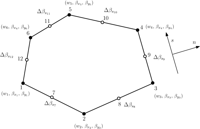
Figure 2: A schematic representation of dofs of a generic polygonal element: kinematic variables at the corner nodes (‘filled circles’) $(w_{i},\beta_{x_{i}},\beta_{y_{i}})$ and temporary variable at the mid-side node (‘open circles’) $\Delta\beta_{s_{k}}$. ‘$(n,s)$’ are the local coordinates defined along each edge of the polygonal element.

Fig. 2 shows a representative polygonal element and the corresponding dofs. For the rotations, an incomplete quadratic field is considered in terms of the rotations at the four corners and temporary variable $\Delta\beta_{sk}$ at the mid-side between two adjacent nodes (see Fig. 2). On each side $i-j$, a local coordinate system is created with $s$ along the edge of the element and $n$ perpendicular to the edge of the element. A linear variation is considered for the normal rotation $\beta_{n}$ whilst a quadratic variation is considered for the tangential component, $\beta_{s}$, given by:

$$\beta_{n} =\left(1-\dfrac{s}{\ell_{k}}\right)\beta_{n_{i}}+\dfrac{s}{\ell_{k}}\beta_{n_{j}}$$

$$\beta_{s} =\left(1-\dfrac{s}{\ell_{k}}\right)\beta_{s_{i}}+\dfrac{s}{\ell_{k}}\beta_{s_{j}}+4\Delta\beta_{s_{k}}$$ (6)

where $\ell_{k}$ is the length of side $i-j$. With these definitions, the transverse displacement, $w$ and the rotations $\beta_{x}$ and $\beta_{y}$ for an element are written as:

$$w =\sum\limits_{i}^{N_{v}}\lambda_{i}w_{i}$$

$$\beta_{x} =\sum\limits_{i}^{N_{v}}\lambda_{i}\beta_{x_{i}}+\sum\limits_{k}^{N_{v}}\psi_{k}C_{k}\Delta\beta_{s_{k}}$$

$$\beta_{y} =\sum\limits_{i}^{N_{v}}\lambda_{i}\beta_{y_{i}}+\sum\limits_{k}^{N_{v}}\psi_{k}S_{k}\Delta\beta_{s_{k}}$$ (7)

where $N_{v}$ is the number of vertices of an element, $\phi_{i}$ and $\psi_{k}$ are the Wachspress interpolants and the serendipity shape functions for an arbitrary polygon, respectively, $C_{k}=(x_{j}-x_{i})/\ell_{k}$ and $S_{k}=(y_{j}-y_{i})/\ell_{k}$ are the directional cosines of side $i-j$. Appendix A gives a brief explanation of Wachspress interpolants.

Upon substituting Equation (7) in Equation (3), we get:

$$\bm{\varepsilon}_{b}=\mathbf{B}_{b_{\beta}}\mathbf{u}+\mathbf{B}_{b_{\Delta\beta}}\bm{\Delta\beta}_{s_{n}}$$ (8)

where $\mathbf{u}=\left\{w\quad\beta_{x}\quad\beta_{y}\right\}$ and $\bm{\Delta\beta}_{s_{n}}$ is the vector of dofs corresponding to the corner nodes and mid-side nodes, respectively, and,

$$\mathbf{B}_{b_{\beta}} =\left[\begin{array}[]{ccc}0&N_{i,x}&0\\ 0&0&N_{i,y}\\ 0&N_{i,y}&N_{i,x}\end{array}\right],\qquad i=1,\cdots,N_{v},$$ (12)

$$\mathbf{B}_{b_{\Delta\beta}} =\left[\begin{array}[]{c}\psi_{k,x}C_{k}\\ \psi_{k,y}S_{k}\\ \psi_{k,y}C_{k}+\psi_{k,x}S_{k}\end{array}\right],\qquad k=1,\cdots,N_{v}$$ (17)

3.1 Assumed shear strain fields

The constitutive equation for the tangential shear strain along a side $k$ joining corner nodes $i,j$ is given by:

$$\overline{\gamma}_{sz}=\dfrac{Q_{s}}{D_{s}}=\dfrac{1}{D_{s}}\left(M_{s,s}+M_{ns,n}\right)$$ (18)

where $D_{s}=\kappa Gh$, $Q_{s}$ is the tangential shear force and the bending moment on each side is given by:

$$M_{s} =D_{b}\left(\beta_{s,s}+\nu\beta_{n,n}\right)$$

$$M_{ns} =D_{b}\dfrac{1-\nu}{2}\left(\beta_{s,n}+\beta_{n,s}\right)$$ (19)

where $D_{b}=\dfrac{Eh^{3}}{12(1-\nu^{2})}$. Using Equations (6) and (19) in Equation (18), the tangential shear strain for an edge $k$ is given by:

$$\overline{\gamma}_{szk}=\dfrac{D_{b}}{D_{s}}\beta_{s,ss}=-\dfrac{4}{3\kappa(1-\nu)}\left(\dfrac{h}{\ell_{k}}\right)^{2}\Delta\beta_{sk}$$ (20)

Next step is to express $\overline{\gamma}_{szk}$ in terms of $\overline{\gamma}_{xzi}$ and $\overline{\gamma}_{yzi}$ using

$$\left\{\begin{array}[]{c}\overline{\gamma}_{szk}\\ \overline{\gamma}_{szm}\end{array}\right\}=\left[\begin{array}[]{cc}C_{k}&S_{k}\\ C_{m}&S_{m}\end{array}\right]\left\{\begin{array}[]{c}\overline{\gamma}_{szi}\\ \overline{\gamma}_{szi}\end{array}\right\}$$ (21)

where $C_{k},S_{k},C_{m}$ and $S_{m}$ are the directional cosines of sides $k$ and $m$ that has a common corner node $i$. This is done for all the sides of the polygonal element. With this definition, the transverse shear strain is interpolated independently with:

$$\left\{\begin{array}[]{c}\overline{\gamma}_{xz}\\ \overline{\gamma}_{yz}\end{array}\right\}=\sum\limits_{i}^{N_{v}}\lambda_{i}\left\{\begin{array}[]{c}\overline{\gamma}_{xzi}\\ \overline{\gamma}_{yzi}\end{array}\right\}$$ (22)

Using Equations (20)-(21), Equation (22) can be written in a compact form as:

$$\overline{\bm{\varepsilon}}_{s}=\mathbf{B}_{s_{\Delta\beta}}\Delta\bm{\beta}$$ (23)

where $\Delta\beta_{s_{n}}$ is the vector of temporary variables of all sides of the polygon and $\mathbf{B}_{s_{\Delta\beta}}$ is a function of the directional cosines, the length of the sides of the element and the plate thickness. An explicit expression for a four noded and a five noded polygonal element is given in Appendix B.

3.2 Discrete constraint on element boundaries

In this paper, the following modified Hu-Washizu functional [26] is used to develop the $n-$noded plate element:

$$\Pi=\dfrac{1}{2}\int\bm{\varepsilon}_{b}^{\rm T}~{}\mathbf{D}_{b}~{}\bm{\varepsilon}_{b}~{}\mathrm{d}\Omega+\dfrac{1}{2}\int\overline{\bm{\varepsilon}}_{s}^{\rm T}\mathbf{D}_{s}\overline{\bm{\varepsilon}}_{s}~{}\mathrm{d}\Omega+\int\mathbf{Q}\left(\bm{\varepsilon}_{s}-\overline{\bm{\varepsilon}}_{s}\right)~{}\mathrm{d}\Omega-\int q~{}w~{}\mathrm{d}\Omega+\Pi_{\rm ext}$$ (24)

where $\Pi_{\rm ext}$ represents the effect of boundary and other loads, $q$ is the transverse loading. Taking the variation of $\Pi$ with respect to $\mathbf{Q}=\left\{Q_{x}\quad Q_{y}\right\}^{\rm T}$ (the shear force) and setting it to zero, we get the following constrain equation:

$$\int\limits_{0}^{\ell_{k}}\left(\gamma_{sz}-\overline{\gamma}_{sz}\right)~{}\mathrm{d}S=0$$ (25)

with $\gamma_{sz}=w_{,s}+\beta_{s}$, where $w$ and $\beta$ are given by Equation (7) and $\overline{\gamma}_{sz}$ is written in terms of $\Delta\beta_{s_{k}}$ using Equation (20). Using Equations (7) and (20) in Equation (25) and upon performing the integration, for a particular edge, $i-j$, we have:

$$w_{j}-w_{i}+\dfrac{\ell_{k}}{2}\left(\beta_{s_{i}}+\beta_{s_{j}}\right)+\dfrac{2}{3}\ell_{k}\Delta\beta_{s_{k}}-\ell_{k}\overline{\gamma}_{szk}=0$$ (26)

Upon substituting Equation (22) in the above equation, we get:

$$w_{j}-w_{i}+\dfrac{\ell_{k}}{2}\left(C_{k}\beta_{x_{i}}+S_{k}\beta_{y_{i}}\right)+\dfrac{\ell_{k}}{2}\left(C_{k}\beta_{x_{j}}+S_{k}\beta_{y_{j}}\right)+\dfrac{2}{3}\ell_{k}(1+\alpha_{k})=0$$ (27)

where $\alpha_{n}=\dfrac{D_{b}}{D_{s}}\dfrac{12}{\ell_{n}^{2}}$. Equation (27) is written for all the sides of the polygonal element to express the temporary variables associated to each edge, $\Delta\beta_{s_{k}}$ in terms of the dofs associated to the corner nodes, as:

$$\Delta\bm{\beta}=\mathbf{A}_{\Delta\beta}^{-1}\mathbf{A}_{2}\mathbf{u}$$ (28)

where,

$$\mathbf{A}_{\Delta\beta}=\begin{bmatrix}\dfrac{2}{3}\ell_{1}(1+\alpha_{1})&0&\dots\\ \vdots&\ddots&\\ 0&&\dfrac{2}{3}\ell_{n}(1+\alpha_{n})\end{bmatrix}$$ (29)

and

$$\mathbf{A}_{2}=\begin{bmatrix}-1&\dfrac{C_{1}}{2}&\dfrac{S_{1}}{2}&1&\dfrac{C_{1}}{2}&\dfrac{S_{1}}{2}&0&\dots&\dots&\dots\\ 0&0&0&-1&\dfrac{C_{2}}{2}&\dfrac{S_{2}}{2}&1&\dfrac{C_{2}}{2}&\dfrac{S_{2}}{2}&\dots\\ \vdots&\vdots&\vdots&\vdots&\vdots&\dots&\dots&\dots&\dots&\vdots\\ -1&\dfrac{C_{n}}{2}&\dfrac{S_{n}}{2}&\dots&\dots&\dots&\dots&1&\dfrac{C_{n}}{2}&\dfrac{S_{n}}{2}\\ \end{bmatrix}$$ (30)

Upon substituting Equation (28) in Equations (8) and (23), the bending strains and the shear strain can be written as:

$$\bm{\varepsilon}_{b} =\mathbf{B}_{b}\mathbf{u}=\left(\mathbf{B}_{b_{\beta}}+\mathbf{B}_{b_{\Delta\beta}}\mathbf{A}_{\Delta\beta}^{-1}\mathbf{A}_{2}\right)\mathbf{u}$$

$$\bm{\varepsilon}_{s} =\mathbf{B}_{s}\mathbf{u}=\left(\mathbf{B}_{s_{\Delta\beta}}\mathbf{A}_{\Delta\beta}^{-1}\mathbf{A}_{2}\right)\mathbf{u}$$ (31)

Finally, using the standard Galerkin approach, the stiffness matrix is a sum of the bending and shear stiffness matrix, given by:

$$\mathbf{K}=\mathbf{K}_{b}+\mathbf{K}_{s}$$ (32)

where

$$\mathbf{K}_{b} =\int\limits_{\Omega}\mathbf{B}_{b}^{\rm T}\mathbf{D}_{b}\mathbf{B}_{b}~{}\mathrm{d}\Omega$$

$$\mathbf{K}_{s} =\int\limits_{\Omega}\mathbf{B}_{s}^{\rm T}\mathbf{D}_{s}\mathbf{B}_{s}~{}\mathrm{d}\Omega$$

The external force vector is computed using the standard finite element procedures. The above formulation allows writing the temporary variable in terms of the dofs associated to the corner nodes. The resulting system of equations has a proper rank and does not have any spurious energy modes. Moreover, as the plate becomes thinner, $\alpha_{k}\ll 1$ and the influence of shear deformations becomes negligible. As a consequence, the proposed formulation does not suffer from shear locking. These aspects are demonstrated with a few benchmark examples in the next section.

4 Numerical Examples

In this section, the accuracy and the convergence properties of the proposed approach are presented with a few benchmark examples. Unless stated otherwise, the material properties of the plate are: Young’s modulus, $E=$ 10.92$\times$10⁶ units and Poisson’s ratio, $\nu=$ 0.3. Both simply supported and clamped boundary conditions are considered. The results from the proposed approach are compared with analytical solutions and/or with results available from the literature. For problems with known analytical solutions, we use the following relative $L^{2}$ norm of the error and the relative $H^{1}-$ semi-norm of the error:

$$\dfrac{||\mathbf{u}-\mathbf{u{{}^{h}}}||_{L^{2}(\Omega)}}{||\mathbf{u}||_{L^{2}(\Omega)}}=\sqrt{\dfrac{\int\limits_{\Omega}(\mathbf{u}-\mathbf{u}^{h})\cdot(\mathbf{u}-\mathbf{u}^{h})~{}\mathrm{d}\Omega}{\int\limits_{\Omega}\mathbf{u}\cdot\mathbf{u}~{}\mathrm{d}\Omega}},$$

$$\dfrac{||\mathbf{u}^{\prime}-\mathbf{u{{}^{{}^{\prime}h}}}||_{H^{1}(\Omega)}}{||\mathbf{u}^{\prime}||_{H^{1}(\Omega)}}=\sqrt{\dfrac{\int\limits_{\Omega}(\mathbf{u}^{\prime}-\mathbf{u}^{{}^{\prime}h})\cdot(\mathbf{u}^{\prime}-\mathbf{u}^{{}^{\prime}h})~{}\mathrm{d}\Omega}{\int\limits_{\Omega}\mathbf{u}^{\prime}\cdot\mathbf{u}^{\prime}~{}\mathrm{d}\Omega}}$$ (33)

where $\mathbf{u}=\left\{w\quad\beta_{x}\quad\beta_{y}\right\}^{\rm T}$ and $\mathbf{u}^{\prime}=\left\{w_{,x}\quad w_{,y}\quad\beta_{x,x}\quad\beta_{x,y}\quad\beta_{y,x}\quad\beta_{y,y}\right\}^{\rm T}$ are the analytical solutions and $\mathbf{u}^{h}$ and $\mathbf{u}^{\prime h}$ are their corresponding FE solutions. The numerical implementation was done in Matlab®. The polygonal mesh generation was done using PolyMesher, available at http://paulino.ce.gatech.edu/software.html.

4.1 Patch test

To ensure that the proposed formulation does not suffer from shear locking phenomenon when the thickness of the plate approaches zero, zero deformation patch test is done [27]. The following exact solution for the transverse displacement and the rotations are enforced on the entire boundary of a square plate with the characteristic length $a=$ 1:

$$w=1+x+y\qquad\beta_{x}=1\qquad\beta_{y}=1$$ (34)

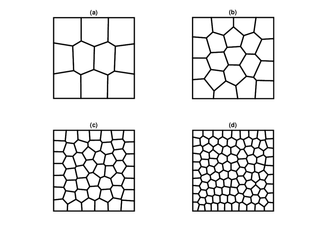
Figure 3: Square plate discretized with trapezoidal mesh and polygonal meshes. Representative meshes containing: (a, c) 16 elements and (b, d) 64 elements. Note that the mid-nodes are not shown for clarity.

Fig. 3 shows a few representative meshes for the square plate discretized with polygonal elements. For different mesh discretization and for different normalized thicknesses, $h/a=$ 0.1, 0.01, 0.001, Tables 1 and 2, shows the relative $L^{2}-$ norm and $H^{1}-$ semi-norm of the error. The errors are close to machine precision for all thickness ratios, $h/a$. It can be concluded that the zero shear deformation patch test is satisfied in the numerical sense and the numerical scheme does not experience the shear locking phenomenon.

Table 1: Relative error in the $L^{2}-$ norm for the zero deformation patch test

Mesh		$h/a$
		0.1	0.01	0.001	0.00001
(a)		2.05$\times$10-14	3.27$\times$10-13	3.68$\times$10-13	6.45$\times$10-13
(b)		1.85$\times$10-14	2.04$\times$10-12	3.07$\times$10-12	6.79$\times$10-13
(c)		1.23$\times$10-13	1.16$\times$10-12	1.67$\times$10-12	3.79$\times$10-12

Table 2: Relative error in the $H^{1}-$ norm for the zero deformation patch test

Mesh		$h/a$
		0.1	0.01	0.001	0.00001
(a)		4.12$\times$10-13	1.17$\times$10-11	6.84$\times$10-12	1.04$\times$10-11
(b)		1.23$\times$10-13	1.16$\times$10-12	1.67$\times$10-12	1.18$\times$10-11
(c)		1.78$\times$10-12	2.86$\times$10-11	4.11$\times$10-11	5.72$\times$10-11

4.2 Square plate subjected to surface load

In this second example, consider a simply supported (or clamped) square plate subjected to uniformly distributed and non-uniformly distributed load. The influence of mesh size and the normalized thickness is studied. The square plate is discretized with arbitrary polygons (see Fig. 3 for representative polygonal meshes).

4.2.1 Plate subjected to uniformly distributed load

In this example, a square plate subjected to a uniformly distributed transverse load $q(x,y)=$ 1 unit is considered with all sides clamped or all sides simply supported boundary conditions. Tables 3 - 4 presents the convergence of the maximum center displacement when the plate is subjected to clamped and simply supported boundary conditions, respectively. Based on a progressive refinement, it can be seen that a mesh of 803 nodes (with 3 dofs per node) is found to be adequate to model the plate. The effect of plate thickness is also studied and it is opined that the present formulation does not suffer from shear locking as the thickness of the plate decreases.

Table 3: Normalized central deflection, $\overline{w}$ for a clamped square plate

Method	$h/a$
	1$\times$10-5	0.001	0.01	0.10	0.15	0.20
Present (104 nodes)	0.1319	0.1319	0.1320	0.1533	0.1815	0.2203
Present (204 nodes)	0.1272	0.1272	0.1273	0.1497	0.1783	0.2174
Present (404 nodes)	0.1276	0.1276	0.1277	0.1511	0.1798	0.2190
Present (602 nodes)	0.1268	0.1268	0.1270	0.1505	0.1791	0.2181
Present (803 nodes)	0.1266	0.1266	0.1267	0.1504	0.1791	0.2181
TTK9s6 [28]	0.1269	0.1269	0.1272	0.1487	0.1746	0.2098
DST-BL [28]	0.1265	0.1265	0.1268	0.1476	0.1726	0.2073
Exact	0.1265	0.1265	0.1265	0.1499	0.1798	0.2167

Table 4: Normalized central deflection, $\overline{w}$ for a simply supported square plate

Method	$h/a$
	1$\times$10-5	0.001	0.01	0.10	0.15	0.20
Present (104 nodes)	0.4013	0.4013	0.4013	0.4199	0.4463	0.4837
Present (204 nodes)	0.3991	0.3991	0.3991	0.4190	0.4457	0.4833
Present (404 nodes)	0.4044	0.4044	0.4044	0.4251	0.4519	0.4896
Present (602 nodes)	0.4042	0.4042	0.4042	0.4250	0.4516	0.4890
Present (803 nodes)	0.4043	0.4043	0.4043	0.4252	0.4520	0.4895
PRMn-W [24]	-	0.4070	-	0.42750	-	-
TTK9s6 [28]	0.4064	0.4064	0.4067	0.4261	0.4507	0.4850
DST-BL [28]	0.4061	0.4061	0.4063	0.4256	0.4501	0.4844
Exact	0.4062	0.4062	0.4064	0.4273	0.4536	0.4906

4.2.2 Plate subjected to a nonuniform load

In this example, we study the convergence properties of the proposed formulation for a square plate subjected to a non-uniformly distributed surface load. The plate is assumed to be clamped on all four sides with side length of the plate, $a=$ 1. The nonuniform surface load is given by:

$$\begin{split}q=\dfrac{E}{12(1-\nu^{2})}\left[12y(y-1)(5x^{2}-5x+1)(2y^{2}(y-1)^{2}+x(x-1)(5y^{2}-5y+1))\right.\\ \left.+12x(x-1)(5y^{2}-5y+1)(2x^{2}(x-1)^{2}+y(y-1)(5x^{2}-5x+1))\right]\end{split}$$ (35)

and the analytical solution for the rotations and the transverse displacement is given by [29]

$$\beta_{x} =-y^{3}(y-1)^{3}x^{2}(x-1)^{2}(2x-1),\quad\beta_{y}=-x^{3}(x-1)^{3}y^{2}(y-1)^{2}(2y-1)$$ (36)

$$w =\dfrac{1}{3}x^{3}(x-1)^{3}y^{3}(y-1)^{3}-\dfrac{2h^{2}}{5(1-\nu)}A_{1}$$ (37)

where $A_{1}=\left[y^{3}(y-1)^{3}x(x-1)(5x^{2}-5x+1)+x^{3}(x-1)^{3}y(y-1)(5y^{2}-5y+1)\right]$. The convergence of the error in the $L^{2}-$norm and $H^{1}-$semi-norm with mesh refinement is shown in Fig. 4 for different plate thickness. It is inferred that the proposed method yields optimal convergence rate in both the norms for different normalized thickness. From Fig. 4, it can further be inferred that the accuracy and the convergence rates are not compromised with the proposed formulation as the plate’s normalized thickness is reduced.

Figure 4: Rates of convergence for the square plate subjected to a non-uniform load: (a) $L_{2}$-norm of the error and (b) $H^{1}$-semi-norm of the error for several values of $h/a$.

4.3 Circular plate subjected to a uniform surface load

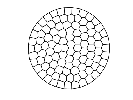
Figure 5: Circular plate: (a) geometry and boundary conditions and (b) representative polygonal discretization

Fig. 5 depicts a circular plate of radius $R=$ 1 subjected to a uniformly distributed surface load, $q(x,y)=$ 1. The plate is assumed to be clamped on the outer boundary. The normalized thickness of the plate is $h/R$. The analytical solution for this problem is given by [8]:

$$w =\dfrac{(x^{2}+y^{2})^{2}}{64D_{b}}-(x^{2}+y^{2})\Bigg{[}\dfrac{t^{2}}{4\lambda}+\dfrac{1}{32D_{b}}\Bigg{]}+\dfrac{t^{2}}{4\lambda}+\dfrac{1}{64D_{b}}$$

$$\beta_{x} =\dfrac{x(x^{2}+y^{2}-1)}{16D_{b}},\quad\beta_{y}=\dfrac{y(x^{2}+y^{2}-1)}{16D_{b}}$$ (38)

Figure 6: Rates of convergence for the circular plate subjected to a uniform load. (a) $L_{2}$-norm of the error and (b) $H^{1}$-semi-norm of the error for several values of $h/a$. DKMT formulation.

The convergence of the relative error is studied for the following normalized thicknesses: $h/R=\left\{0.2,0.1,0.01,0.00001\right\}$. Fig. 6 shows the converges rates for the proposed method and it is inferred that the optimal rates of convergence is obtained in both the $L^{2}$ norm and $H^{1}$ semi-norm for all thickness ratios. It can be opined that the proposed method does not suffer from shear locking.

5 Conclusions

In this paper, the discrete Kirchhoff Mindlin theory is applied to arbitrary polygons using the primary unknowns, viz., the transverse displacements and the rotations. The transverse shear effect is included by assuming that the tangential shear strain is constant along each edge of the polygon. The shear locking phenomenon is then alleviated by relating the kinematical and the independent shear strain along each edge of the polygon. With a few examples, we have shown that the proposed formulation passes patch test to machine precision, devoid of shear locking phenomenon and yields optimal convergence rates for both thin and thick plates in $L^{2}-$norm and $H^{1}-$semi-norm.

Appendix A

Wachspress interpolants

Wachspress [30], by using the principles of perspective geometry, proposed rational basis functions on polygonal elements, in which the algebraic equations of the edges are used to ensure nodal interpolation and linearity on the boundaries.

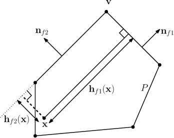
Figure 7: Barycentric coordinates: Wachspress basis function

The generalization of Wachspress shape functions to simplex convex polyhedra was given by Warren [31, 32]. The construction of the coordinates is as follows: Let $P\subset{\rm{I\!R}}^{3}$ be a simple convex polyhedron with facets $F$ and vertices $V$. For each facet $f\in F$, let $\bm{\mathrm{n}}_{f}$ be the unit outward normal and for any $\bm{\mathrm{x}}\in P$, let $h_{f}(\bm{\mathrm{x}})$ denote the perpendicular distance of $\bm{\mathrm{x}}$ to $f$, which is given by

$$h_{f}(\bm{\mathrm{x}})=(\mathbf{v}-\bm{\mathrm{x}})\cdot\bm{\mathrm{n}}_{f}$$ (39)

for any vertex $\mathbf{v}\in V$ that belongs to $f$. For each vertex $\mathbf{v}\in V$, let $f_{1},f_{2},f_{3}$ be the three faces incident to $\mathbf{v}$ and for $\bm{\mathrm{x}}\in P$, let

$$w_{\mathbf{v}}(\bm{\mathrm{x}})=\frac{\mathrm{det}(\bm{\mathrm{p}}_{f_{1}},\bm{\mathrm{p}}_{f_{2}},\bm{\mathrm{p}}_{f_{3}})}{h_{f_{1}}(\bm{\mathrm{x}})h_{f_{2}}(\bm{\mathrm{x}})h_{f_{3}}(\bm{\mathrm{x}})}.$$ (40)

where, $\bm{\mathrm{p}}_{f}:=\bm{\mathrm{n}}_{f}/h_{f}(\bm{\mathrm{x}})$ is the scaled normal vector, $f_{1},f_{2},\cdots,f_{d}$ are the $d$ faces adjacent to $\bm{\mathrm{v}}$ listed in an counter-clockwise ordering around $\bm{\mathrm{v}}$ as seen from outside $P$ (see Fig. 7) and $det$ denotes the regular vector determinant in $\mathbb{R}^{d}$. The shape functions for $\bm{\mathrm{x}}\in P$ is then given by

$$\lambda{\mathbf{v}}(\bm{\mathrm{x}})=\frac{w_{\mathbf{v}}(\bm{\mathrm{x}})}{\sum\limits_{\mathbf{u}\in V}w_{\mathbf{u}}(\bm{\mathrm{x}})}.$$ (41)

The Wachspress shape functions are the lowest order shape functions that satisfy boundedness, linearity and linear consistency on convex polyshapes [31, 32]. A simple MATLAB implementation is given in [33] along with the gradient bounds for Wachspress coordinates. A discussion on their use for smoothed polygonal elements is given in [34].

Quadratic serendipity shape functions

In this work, the quadratic serendipity shape functions are constructed from pairwise product of set of barycentric coordinates [35]. These shape functions are $\mathit{C}^{\infty}$ continuous inside the domain $\Omega$ while $\mathit{C}^{0}$ continuous at the boundary $\Gamma$. The pairwise product of a set of barycentric coordinates ($\lambda_{i}$), yields a total of $n(n+1)/2$ functions with mid-nodes on the edges and nodes inside the domain. Then by appropriate linear transformation technique, the $n(n+1)/2$ set of functions are reduced to $2n$ set of functions that satisfies Lagrange property. The essential steps involved in the construction of quadratic serendipity shape functions are (also see Fig. 8:

1. Select a set of barycentric coordinates $\phi_{i},i=1,\cdots,n$, where $n$ is the number of vertices of the polygon.

2. Compute pairwise functions $\mu_{ab}:={\phi_{a}\phi_{b}}$. This construction yields a total of $n(n+1)/2$ functions.

3. Apply a linear transformation $\mathbb{A}$ to $\mu_{ab}$. The linear transformation $\mathbb{A}$ reduces the set $\mu_{ab}$ to $2n$ set of functions $\xi_{ij}$ indexed over vertices and edge midpoints of the polygon.

4. Apply another linear transformation $\mathbb{B}$ that converts $\xi_{ij}$ into a basis $\psi_{ij}$ which satisfies the “Lagrange property.”

Interested readers are referred to [35] for a detailed discussion on the construction of quadratic serendipity elements.

Figure 8: Construction of quadratic serendipity shape functions based on generalized barycentric coordinates.

Appendix B

Fig. 9 shows a generic quadrilateral and a pentagonal element. The shear strain-displacement matrix $\mathbf{B}_{s_{\Delta\beta}}$ (c.f. Equation (23)) is given by:

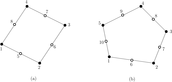
Figure 9: A generic polygonal element.

For a quadrilateral element

$$\mathbf{B}_{s_{\Delta\beta}}=-\dfrac{2}{3}\begin{bmatrix}\left(\dfrac{S_{8}}{A_{1}}\lambda_{1}-\dfrac{S_{6}}{A_{2}}\lambda_{2}\right)&\left(-\dfrac{C_{8}}{A_{1}}\lambda_{1}-\dfrac{C_{6}}{A_{2}}\lambda_{2}\right)\\ \left(\dfrac{S_{5}}{A_{2}}\lambda_{2}-\dfrac{S_{7}}{A_{3}}\lambda_{3}\right)&\left(-\dfrac{C_{5}}{A_{2}}\lambda_{2}-\dfrac{C_{7}}{A_{3}}\lambda_{3}\right)\\ \left(\dfrac{S_{6}}{A_{3}}\lambda_{3}-\dfrac{S_{8}}{A_{4}}\lambda_{4}\right)&\left(-\dfrac{C_{6}}{A_{3}}\lambda_{3}-\dfrac{C_{8}}{A_{4}}\lambda_{4}\right)\\ \left(\dfrac{S_{7}}{A_{4}}\lambda_{4}-\dfrac{S_{5}}{A_{1}}\lambda_{1}\right)&\left(-\dfrac{C_{7}}{A_{4}}\lambda_{4}-\dfrac{C_{5}}{A_{1}}\lambda_{1}\right)\end{bmatrix}^{\rm T}$$

and for a pentagonal element

$$\mathbf{B}_{s_{\Delta\beta}}=-\dfrac{2}{3}\begin{bmatrix}\left(\dfrac{S_{10}}{A_{1}}\lambda_{1}-\dfrac{S_{7}}{A_{2}}\lambda_{2}\right)&\left(-\dfrac{C_{10}}{A_{1}}\lambda_{1}-\dfrac{C_{7}}{A_{2}}\lambda_{2}\right)\\ \left(\dfrac{S_{6}}{A_{2}}\lambda_{2}-\dfrac{S_{8}}{A_{3}}\lambda_{3}\right)&\left(-\dfrac{C_{6}}{A_{2}}\lambda_{2}-\dfrac{C_{8}}{A_{3}}\lambda_{3}\right)\\ \left(\dfrac{S_{7}}{A_{3}}\lambda_{3}-\dfrac{S_{9}}{A_{4}}\lambda_{4}\right)&\left(-\dfrac{C_{7}}{A_{3}}\lambda_{3}-\dfrac{C_{9}}{A_{4}}\lambda_{4}\right)\\ \left(\dfrac{S_{8}}{A_{4}}\lambda_{4}-\dfrac{S_{10}}{A_{5}}\lambda_{5}\right)&\left(-\dfrac{C_{8}}{A_{4}}\lambda_{4}-\dfrac{C_{10}}{A_{5}}\lambda_{5}\right)\\ \left(\dfrac{S_{9}}{A_{5}}\lambda_{5}-\dfrac{S_{6}}{A_{1}}\lambda_{1}\right)&\left(-\dfrac{C_{9}}{A_{5}}\lambda_{5}-\dfrac{C_{6}}{A_{2}}\lambda_{2}\right)\end{bmatrix}^{\rm T}$$

where $\lambda_{i}$ are the Wachspress interpolants.

References

References

- Zienkiewicz et al. [1971] O. Zienkiewicz, R. Taylor, J. Too, Reduced integration technique in general analysis of plates and shells, International Journal for Numerical Methods in Engineering 3 (1971) 275–290.
- Hughes et al. [1978] T. Hughes, M. Cohen, M. Haroun, Reduced and selective integration techniques in the finite element analysis of plates, Nuclear Engineering and Design 46 (1978) 203–222.
- Malkus and Hughes [1978] D. Malkus, T. Hughes, Mixed finite element methods - reduced and selective integration techniques: a unification of concepts, Computer Methods in Applied Mechanics and Engineering 15 (1978) 63–81.
- Belytschko et al. [1981] T. Belytschko, C. Tay, W. Liu, A stabilization matrix for the bilinear Mindlin plate element, Computer Methods in Applied Mechanics and Engineering 29 (1981) 313–327.
- Bathe and Dvorkin [1985] K. Bathe, E. Dvorkin, A four-node plate bending element based on mindlin-reissner plate theory and a mixed interpolation, International Journal for Numerical Methods in Engineering 21 (1985) 367–383.
- Bletzinger et al. [2000] K.-U. Bletzinger, M. Bischoff, E. Ramm, A unified approach for shear-locking-free triangular and rectangular shell elements, Computers & Structures 75 (2000) 321–334.
- Spilker and Munir [1980] R. Spilker, N. Munir, The hybrid-stress model for thin plates, International Journal for Numerical Methods in Engineering 15 (1980) 1239–1260.
- Katili [1993] I. Katili, A new discrete Kirchhoff-Mindlin element based on Mindlin-Reissner plate theory and assumed shear strain fields - Part II: An extended DKQ element for thick-plate bending analysis, International Journal for Numerical Methods in Engineering 36 (1993) 1885–1908.
- Cen and Shang [2015] S. Cen, Y. Shang, Developments of mindlin-reissner plate elements, Mathematical Problems in Engineering Article ID 456740 (2015).
- Lipnikov and Manzini [2014] K. Lipnikov, G. Manzini, A high-order mimetic method on unstructured polyhedral mesh for the diffusion equation, Journal of Computational Physics 272 (2014) 360–385.
- da Veiga and Manzini [2012] L. B. da Veiga, G. Manzini, The mimetic finite difference method and the virtual element method for elliptic problems with arbitrary regularity, Technical Report LA-UR-12-22977, Los Alamos National Laboratory, 2012.
- da Veiga et al. [2013] L. B. da Veiga, F. Brezzi, A. Cangiani, G. Manzini, L. D. Marini, A. Russo, Basic principles of virtual element methods, Mathematical Models and Methods in Applied Sciences 23 (2013) 199–214.
- da Veiga et al. [2014] L. B. da Veiga, F. Brezzi, L. D. Marini, A. Russo, The hitchhiker’s guide to the virtual element method, Mathematical Models and Methods in Applied Sciences 24 (2014) 1541–1573.
- Droniou [2010] J. Droniou, Finite volume schemes for diffusion equation: Introduction to and review of modern methods, Mathematical Models and Methods in Applied Sciences 24 (2010) 1575–1619.
- Cangiani et al. [2014] A. Cangiani, E. H. Georgoulis, P. Houston, hp-version discontinuous galerkin methods on polygonal and polyhedral meshes, Mathematical Models and Methods in Applied Sciences 24 (2014) 2009–2041.
- hai Tang et al. [2009] X. hai Tang, S.-C. Wu, C. Zheng, J. hai Zhang, A novel virtual node method for polygonal elements, Applied Mathematics and Mechanics 30 (2009) 1233–1246.
- Natarajan et al. [2014] S. Natarajan, E. T. Ooi, I. Chiong, C. Song, Convergence and accuracy of displacement based finite element formulation over arbitrary polygons: Laplace interpolants, strain smoothing and scaled boundary polygon formulation, Finite Elements in Analysis and Design 85 (2014) 101–122.
- Ooi et al. [2016] E. Ooi, C. Song, S. Natarajan, Construction of high-order complete scaled boundary shape functions over arbitrary polygons with bubble functions, International Journal for Numerical Methods in Engineering 108 (2016) 1086–1120.
- Natarajan et al. [2017] S. Natarajan, E. T. Ooi, A. Saputra, C. Song, A scaled boundary finite element formulation over arbitrary faceted star convex polyhedra, Engineering Analysis with Boundary Elements 80 (2017) 218–229.
- Biabanaki and Khoei [2012] S. O. R. Biabanaki, A. R. Khoei, A polygonal finite element method for modeling arbitrary interfaces in large deformation problems, Computational Mechanics 50 (2012) 19–33.
- Talischi et al. [2014] C. Talischi, A. Pereira, G. H. Paulino, I. F. M. Menezes, M. S. Carvalho, Polygonal finite elements for incompressible fluid flow, International Journal for Numerical Methods in Engineering 74 (2014) 134–151.
- Biabanaki et al. [2014] S. Biabanaki, A. R. Khoei, P. Wriggers, Polygonal finite element methods for contact-impact problems on non-conformal meshes, Computer Methods in Applied Mechanics and Engineering 269 (2014) 198–221.
- Khoei et al. [2015] A. R. Khoei, R. Yasbolaghi, S. Biabanaki, A polygonal finite element method for modeling crack propogation with minimum remeshing, International Journal of Fracture 194 (2015) 123–148.
- Nguyen-Xuan [2017] H. Nguyen-Xuan, A polygonal finite element method for plate analysis, Computers & Structures 188 (2017) 45–62.
- Batoz and Tahar [1982] J.-L. Batoz, M. B. Tahar, Evaluation of a new thin plate quadrilateral element, International Journal for Numerical Methods in Engineering 16 (1982) 1655–1678.
- Batoz and Katili [1992] J.-L. Batoz, I. Katili, On a simple triangular reissner/mindlin plate element based on incompatible modes and discrete constraints, International Journal for Numerical Methods in Engineering 35 (1992) 1603–1632.
- Chen et al. [2009] W. Chen, J. Wang, J. Zhao, Functions for patch test in finite element analysis of the Mindlin plate and the thin cylindrical shell, Sci. China Ser. G 52 (2009) 762–767.
- Zhuang et al. [2013] X. Zhuang, R. Huang, H. Zhu, H. Askes, K. Mathisen, A new and simple locking-free triangular thick plate element using independent shear degrees of freedom, Finite Elements in Analysis and Design 75 (2013) 1–7.
- Chinosi and Lovadina [1995] C. Chinosi, C. Lovadina, Numerical analysis of some mixed finite element methods for Reissner-Mindlin plates, Computational Mechanics 16 (1995) 36–44.
- Wachspress [1971] E. Wachspress, A rational basis for function approximation, Springer, New York, 1971.
- Warren [2003] J. Warren, On the uniqueness of barycentric coordinates, in: Proceedings of AGGM02, pp. 93–99.
- Warren et al. [2007] J. Warren, S. Schaefer, A. Hirani, M. Desbrun, Barycentric coordinates for convex sets, Advances in Computational Mechanics 27 (2007) 319–338.
- Floater et al. [2014] M. Floater, A. Gillette, N. Sukumar, Gradient bounds for Wachspress coordinates on polytopes, SIAM J. Numer. Anal. 52 (2014) 515–532.
- Bordas and Natarajan [2010] S. Bordas, S. Natarajan, On the approximation in the smoothed finite element method (SFEM), International Journal for Numerical Methods in Engineering 81 (2010) 660–670.
- Rand et al. [2014] A. Rand, A. Gillette, C. Bajaj, Quadratic serendipity finite elements on polygons using generalized barycentric coordinates, Mathematics of Computation 83 (2014) 2691–2716.