Nutation dynamics and multifrequency resonance in a many-body seesaw

Abstract

The multifrequency resonance has been widely explored in the context of single-particle models, of which the modulating Rabi model has been the most widely investigated. It has been found that with diagonal periodic modulation, steady dynamics can be realized in some well-defined discrete frequencies. These frequencies are independent of off-diagonal couplings. In this work, we generalize this physics to the many-body seesaw realized using the tilted Bose–Hubbard model. We find that the wave function will recover to its initial condition when the modulation frequency is commensurate with the initial energy level spacing between the ground and the first excited levels. The period is determined by the driving frequency and commensurate ratio. In this case, the wave function will be almost exclusively restricted to the lowest two instantaneous energy levels. By projecting the wave function to these two relevant states, the dynamics is exactly the same as that for the spin precession dynamics and nutation dynamics around an oscillating axis. We map out the corresponding phase diagram, and show that, in the low-frequency regime, the state is thermalized, and in the strong modulation limit, the dynamics is determined by the effective Floquet Hamiltonian. The measurement of these dynamics from the mean position and mean momentum in phase space are also discussed. Our results provide new insights into multifrequency resonance in the many-body system.

The multifrequency resonance has been widely explored in some of the single-particle models Haroche et al. (1970); Smeltzer et al. (2009); Steiner et al. (2010), in which the two-level Rabi model subjects to diagonal modulation was most widely investigated Miao and Zheng (2016); Yan et al. (2017); Nakamura et al. (2001); Longhi (2006). The simplest model for this mechanism can be written as Miao and Zheng (2016); Ashhab et al. (2007); Oliver et al. (2005)

$$H=-\frac{\Delta}{2}\sigma_{x}-\frac{\varepsilon(t)}{2}\sigma_{z},$$ (1)

where $\Delta$ is the coupling strength between the ground state and excited state, $\varepsilon(t)$ is the time-dependent bias, and $\sigma_{x}$ and $\sigma_{z}$ are Pauli matrices. We can choose

$$\varepsilon(t)=\epsilon_{0}+A\cos(\omega t),$$ (2)

where $A$ is the driving amplitude, $\varepsilon_{0}$ is the static detuning and $\omega$ is the modulation frequency. The Schrödinger equation for $H$ can be written as $i\partial_{t}|\psi\rangle=H|\psi\rangle$. We can choose a rotating operator as

$$U(t)=\exp[{i\over 2}(\varepsilon_{0}t+{A\over\omega}\sin(\omega t))\sigma_{z}],$$ (3)

and write the wave function as $|\psi\rangle=U(t)|\psi_{\text{r}}\rangle$, where $|\psi_{\text{r}}\rangle$ is the wave function in the rotating frame. We find that $i\partial_{t}|\psi_{\text{r}}\rangle=H^{\text{r}}|\psi_{\text{r}}\rangle$, with

$$H^{\text{r}}=U^{\dagger}(t)HU(t)-iU^{\dagger}(t)\frac{dU(t)}{dt}=-\frac{\Delta}{2}\left(\begin{array}[]{cc}0&Q\\ Q^{*}&0\end{array}\right),$$ (4)

where $Q=\sum_{n=-\infty}^{\infty}J_{n}\left(\frac{A}{\omega}\right)e^{-i\left(n\omega+\varepsilon_{0}\right)t}$, with $J_{n}(x)$ being the Bessel function of the first kind. Steady dynamics can be realized when $n\omega+\varepsilon_{0}=0$ for some integer $n$, which yields multifrequency resonance. This resonance is independent of the off-diagonal coupling $\Delta$. Since the above Rabi model can be readily realized using some of the quantum simulators, this physics has been implemented in superconducting qubits Sillanpää et al. (2006); Izmalkov et al. (2008); Wilson et al. (2010); Sun et al. (2011), ultracold atoms Felicetti et al. (2017), and NV color centers Childress and McIntyre (2010); Jiang et al. (2009); Neumann et al. (2008); London et al. (2013). An intensive review of this physics in the Rabi model can be found in Ref. Xie et al. (2017). This method has also been applied in medicine for magnetic resonance imaging Eles and Michal (2010); Han and Liu (2020). Moreover, the similar physics can also be found in the other models without these energy levels, such as the nonlinear oscillator Testa et al. (1982); Richetti et al. (1986); Paluš and Novotná (1999); Dykman and Fistul (2005), nanomechanical resonators Aldridge and Cleland (2005); Katz et al. (2007), and Josephson junctions Fistul et al. (2003); Siddiqi et al. (2004). However, the physics in the many-body system, which involves much more complicated energy levels, is rarely discussed.

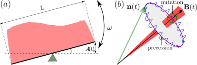
Figure 1: (a) Quantum seesaw model constructed by a finite chain with length $L$ under hard-wall boundary condition. The modulation frequency $\omega$, inclination $\alpha$ are controllable in experiments. The change of potential at the two ends is $A(t)=\alpha\sin(\omega t)\frac{L}{2}$. (b) Nutation and precession dynamics for a spin about an modulating magnetic field. The corresponding spin vector is defined as ${\bf n}(t)=\langle\psi(t)|\boldsymbol{\sigma}|\psi(0)\rangle$, where $\boldsymbol{\sigma}$ are Pauli matrices. Here the smaller, faster, periodic oscillation is called the nutation dynamics, while the slower one is called the precession dynamics.

In this work, we generalize this concept to the realm of many-body physics based on a modulating quantum seesaw realized by the Bose-Hubbard model, in which some new dynamics beyond the above single-particle picture can be realized. We find that: (I) When the modulation frequency is commensurate with the level spacing between the ground state and the first excited state of the Hamiltonian at time $t=0$, periodic recovery of the wave function can be realized, with a period determined by the tunable commensurate ratio $\beta$. (II) By projecting the wave function to the two lowest states, the many-body dynamics is reduced to a spin model precession about an oscillating magnetic field, which yields a new mechanism to the realization of the multifrequency resonance via nutation dynamics Driben et al. (2016); Ciornei et al. (2011). This picture even has a single-particle and classical analogous. (III) This phase can be realized only when the commensurate ratio is large enough. In the low modulation limit beyond the adiabatic limit, the many-body state will quickly approaches the thermalized state. In the high-frequency limit, this nutation dynamics is suppressed, and the dynamics is determined by the Floquet Hamiltonian. We have also discussed the experimental detection of these phases and discuss their stability with non-integrability interactions. Our results are stimulating for the exploring of the multifrequency resonance in the many-body system.

Physical model and dynamics. We consider the following driven Bose-Hubbard model in a finite chain

$$H =-J\sum_{i=1}^{L-1}(b_{i}^{\dagger}b_{i+1}+\text{h.c.})+\frac{U}{2}\sum_{i=1}^{L}n_{i}(n_{i}-1)$$ (5)

$$+\alpha\sum_{i=1}^{L}\sin(\omega t)(i-{L+1\over 2})n_{i},$$

which is schematically shown in Fig. 1. Here $b_{i}^{\dagger}$ $(b_{i})$ are the creation (annihilation) operators at the $i$-th lattice site, $n_{i}=b_{i}^{\dagger}b_{i}$ is the number operator, $J$ is the tunneling strength and $U>0$ is the on-site many-body interaction. In following, we set $J=1$ as the basic energy scale. In experiments, $J\sim 2\pi\times\mathcal{O}(0.1)$ kHz Dai et al. (2017); Trotzky et al. (2012); Bukov et al. (2015); Pigneur et al. (2018). The last term represents the quantum seesaw, which can be realized by a tilted magnetic field with modulation frequency $\omega$ and inclination $\alpha$. This tilted potential has been realized in experiments Simon et al. (2011); Preiss et al. (2015); Geiger et al. (2018); Kennedy et al. (2015). The hard wall boundary condition has been realized with a box potential in several groups, with $L$ typically from 10 to 100 Lopes et al. (2017); Gaunt et al. (2013); Mukherjee et al. (2017); Eigen et al. (2016). The data we will present are obtained by exact diagonalization (ED) and time-evolving block decimation (TEBD) methods Vidal (2003, 2004). In the simulation, we choose $\omega=\beta\Delta E_{12}$, where $\Delta E_{12}=E_{2}-E_{1}$ is the level spacing between the ground state and first excited state of $H(t=0)$ and $\beta$ is a rational number termed as the commensurate ratio.

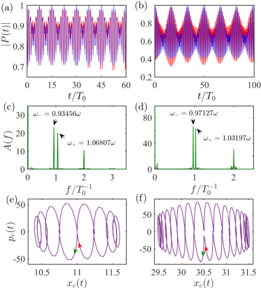
Figure 2: (a) - (b) Periodically recovery of wave function. (a) Red line for $L=21$, $\beta=15$, $N=10$, $U=\sqrt{2}$, $\alpha=1/3$ and blue dotted line is given by Eq. 9, for $g=1.27$, $A=\lambda=0$, $\epsilon=\Delta E_{12}/2$. (b) Red line for $L=60$, $\beta=33$, $N=35$, $U=0.8$, $\alpha=0.05$ and blue dotted line for $g=1.83$, $A=\lambda=0$, $\epsilon=\Delta E_{12}/2$. (c)-(d) Fourier spectroscopy of $P(t)$. The arrows correspond to $\omega_{\pm}=\omega\pm\omega^{\prime}$. (e)-(f) Trajectory in phase space by mean position and mean momentum. The arrows indicate the direction of the time evolution.

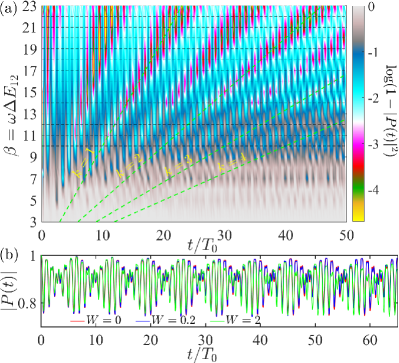
Figure 3: (a). The probability $|P(t)|^{2}$ as a function of $\beta$ and $t/T_{0}$ with $L=21$, $N=10$, $U=\sqrt{2}$, $\alpha=1/(3\sqrt{5})$. The green dashed lines are given by $t/T_{0}=k\beta$, where $k=1$, 2 , 3, $\cdots$. (b). The influence of disorder in the multifrequency resonance phase with $L=12$, $N=5$, $U=0.8$, $\alpha=0.3$. For different disorder strength, we fixed driving frequency $\omega=13\Delta E_{12}$, where the $\Delta E_{12}$ is given by $W=0$ and averaged by 10 realizations.

Let us first consider the dynamics in a short chain ($L=21$, $\beta=15$) and a long chain ($L=60$, $\beta=33$) in Fig. 2. The same physics can be found by choosing some other parameters. To measure whether the wave function will recover to its initial state $|\psi(0)\rangle$ (the ground state of $H(t=0)$), we measure the overlap between them via $P(t)=\langle\psi(0)|\psi(t)\rangle$ Heyl et al. (2013); Jurcevic et al. (2017) (see Fig. 2(a) - (b)), which is related to the Ramsey interferometry in experiments Goold et al. (2011); Knap et al. (2012); Cetina et al. (2016). To determine the period, we have also calculated the Fourier transition of this recovery probability (see Fig. 2(c) - (d)). In both cases, the wave function will almost recover to its initial state with $|P|>93\%$. This period can be precisely determined by the Fourier spectra in the time domain with two frequencies $\omega_{\pm}=\omega\pm\omega^{\prime}$, where $\omega$ is the driving frequency of the seesaw. We find that $T=2\pi/\omega^{\prime}=\beta T_{0}$, with $T_{0}=2\pi/\omega$ being the period of the driving field. This dynamics can persist for an extraordinarily long time. Here we only consider the case that $\beta$ to be integer values for simplicity, and a more general proof will be presented below, from which our conclusion is also true for rational numbers.

To detect this dynamics, we investigate the mean position $x_{c}$ and mean momentum $p_{c}$ in the phase space in Fig. 2(e) - (f), by defining $x_{c}(t)=\sum_{m}\langle\psi(t)|b_{m}^{\dagger}b_{m}|\psi(t)\rangle m/N$, where $N$ is the total number of particles and $p_{c}(t)=\text{d}x_{c}(t)/\text{d}t$ (we have used $\text{d}t=0.001$ in the calculation of $p_{c}$). In the phase space, these two variables construct an almost closed trajectory after one period $T$. For the two sets of parameters in Fig. 2, the real space displacement is roughly one or two lattice sites, and the change of mean momentum is slightly larger (in the standard unit of momentum) than this value. These two variables can be measured in both real and momentum spaces from the time-of-flight spectroscopy Wang et al. (2012); Hart et al. (2015); Atala et al. (2013); Anderlini et al. (2007).

In order to more clearly see the relationship between the driving frequency and the response period, we plot the recovery probability in Fig. 3(a). When $\beta$ is small, we find a regime with complicated dynamics; however, with the increasing of $\beta$, the periodic modulation of $|P(t)|^{2}$ can be observed as a function of evolution time. We find that when $t/T_{0}=k\beta$ $(k=1,2,3,\cdots)$, the probability $|P(t)|^{2}$ will approaches a peak with the largest recovery $|P|\rightarrow 1$. That means the response period $T=\beta T_{0}$.

The influence of disorder. Next, we consider the influence of on-sites disorder for the multifrequency resonance phase. We introduce the disordered term $H_{D}=\sum_{i}^{L}h_{i}n_{i}$ in Eq. 5, where $h_{i}\in[-W,W]$ and $W$ is the disorder strength. This is a typical term to break the integrability of the Bose-Hubbard model. We choose $L=12$, $N=5$, $U=0.8$, $\alpha=0.3$ with fixed frequency $\omega=13\Delta E_{12}$, where the $\Delta E_{12}$ is the gap of Eq. 5 at $t=0$. The results are shown in Fig. 3(b) averaged by 10 realizations. In our model, the recovery period is strongly dependents on the energy gap of the system parameters at the initial moment. Therefore, for weak disorder strength, $W=0.2$, we can see that the curve almost coincides with $W=0$, because the gap is almost unchanged. However, for strong disorder strength, $W=2$, the gap will be changed, so, the curve is significantly different from $W=0$ at long time. However, the periodical recovery of the probability can still be seen clearly, indicating that the dynamics is robust against disorder and the related non-integrability interactions.

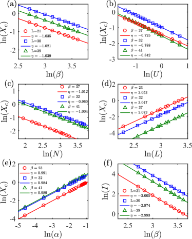
Figure 4: (a) - (e) The maximal displacement $X_{c}$ (see Eq. 6) as a function of $\beta$, $U$, $N$, $L$ and $\alpha$. (f) The area enclosed by the trajectory in phase space as a function of $\beta$. Parameters for open symbols $\bigcirc$ are $L=21$, $N=10$, $U=\sqrt{2}$, $\alpha=1/(3\sqrt{5})$; $\square$ are $L=30$, $N=15$, $U=0.8$, $\alpha=0.1$ and $\bigtriangleup$ are $L=39$, $N=22$, $U=\sqrt{3}/2$, $\alpha=0.05$.

The influence of parameters on the measurement. We next explore how the parameters influence the mean position displacement, by defining

$$X_{c}=\frac{\text{max}(x_{c})-\text{min}(x_{c})}{2}\sim s^{\eta},$$ (6)

where $s$ may refer to $\beta$, $U$, $N$, $L$, $\alpha$ etc.. The exponents for these five cases are $\eta\simeq-1.0,-0.8,-1.0$, $3.0$ and $1.0$, respectively; see Fig. 4(a) - (e). This means, in experiments, the larger center of mass displacement can be found with relatively smaller modulation frequency, interaction strength and total number of particles, and relatively larger number of lattice site $L$ and inclination $\alpha$. We also measure the area of the trajectory enclosed by $p_{c}$ and $x_{c}$ using $I=\frac{1}{2\pi}\oint p_{c}\text{d}x_{c}\sim s^{\eta}$. This quality has a number of interesting features. In the adiabatic limit, it should be quantized (in the unit of Planck constant), which has played a fundamental role in history in the development of quantum theory and quantization condition in Sommerfeld theory. In Fig. 4(f), we find that $I$ has the same scaling as Eq. 6 with exponent $\eta\simeq-3.0$. This value is not quantized due to non-adiabatic evolution.

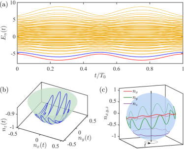
Figure 5: (a) Instantaneous eigenvalues for $L=7,N=3,U=0.8,\alpha=0.5,\omega=11\Delta E_{12}$ and $\Delta E_{12}=0.518804$. (b) The dynamics of the spin vector ${\bf n}$ in the Bloch sphere, with $A=\lambda=0,g=\sqrt{2},\epsilon=0.53,\omega=10\Delta E_{12}$. (c) The corresponding precession and nutation dynamics in the three directions, with the arrow marks the evolution in one full period.

Mapping to a spin vector about an oscillating magnetic field. This model provides a new mechanism for the realization of multifrequency resonance with a controllable commensurate period, which will be termed as multifrequency resonance phase. To pin down the underlying mechanism for this dynamics, we now project the wave function $\psi(t)$ from the time-dependent Schrödinger equation to the instantaneous eigenstates $\phi_{n}$, where $H(t)\phi_{n}(t)=\epsilon_{n}(t)\phi_{n}(t)$ with $\epsilon_{n}$ to be arranged in increasing order. The idea is quite similar to the derivation of geometry phase in topological physics Berry (1985, 2009); del Campo (2013); Aharonov and Casher (1984), but now we need to consider a few low-lying eigenstates as

$$\psi(t)=c_{1}\phi_{1}(t)+c_{2}\phi_{2}(t)+\cdots.$$ (7)

We will focus on the regime when $\omega$ is smaller than the whole bandwidth (see the eigenvalues of $H(t)$ in Fig. 5(a), with bandwidth $W_{b}=\text{max}(\epsilon_{n})-\text{min}(\epsilon_{n})=11.33844$). We find that $|c_{1}|^{2}+|c_{2}|^{2}$ is always larger than 0.9, indicating that almost all the wave functions, during the long-time evolution, is almost restricted to the lowest two instantaneous eigenstates. In this way, we can keep only these two major terms. Then $\psi(t)$ can be the solution of the Schrödinger equation corresponding to the following equivalent Hamiltonian,

$$\mathcal{H}_{\text{eq}}(t)=\varepsilon(t)+b^{i}(t)\sigma_{i}=\varepsilon(t)+{\bf B}(t)\cdot\boldsymbol{\sigma},$$ (8)

where the Pauli matrices act on the subspace constructed by the lowest two states in Eq. 7 and ${\bf B}=(b^{x},b^{y},b^{z})$. In this manner, we map the many-body model to the spin dynamics about an oscillating magnetic field ${\bf B}(t)$, in which the spin exhibits both (slower) precession and (faster) nutation dynamics (see Fig. 1(b)). The nutation dynamics comes from the periodic modulation of the rotating axis. We also describe this dynamics on the Bloch sphere, showing in Fig. 5(b) and the corresponding precession and nutation dynamics in the three directions are shown in Fig. 5(c). This kind of dynamics is analogous to the dynamics in astrophysics Herring et al. (1991); Mathews et al. (2002), in which these two dynamics are prevailing.

For the general case, we let ${\bf B}(t)=(y(t)+\lambda,0,f(t)+\epsilon)$. Let us assume the initial state to be $|\psi(0)\rangle=|\downarrow\rangle$ and to the leading order via perturbation theory we find

$$\left\{\begin{aligned} &|\psi(t)\rangle=\frac{1}{\sqrt{|c_{1}(t)|^{2}+|c_{2}(t)|^{2}}}(c_{1}(t)|\downarrow\rangle+c_{2}(t)|\uparrow\rangle),\\ &c_{1}(t)=1-i\int_{0}^{t}f(t)dt,\quad c_{2}(t)=-i\int_{0}^{t}e^{i\Delta E_{12}t}y(t)dt,\end{aligned}\right.$$ (9)

where $\Delta E_{12}=2\sqrt{\epsilon^{2}+\lambda^{2}}$. If $f(t)$ and $y(t)$ are smooth functions with the same modulating frequency $\omega$, that means $f(t)$ and $y(t)$ have the same period $T_{0}=2\pi/\omega$. On the other hand, $e^{i\Delta E_{12}t}$ has the period $T^{\prime}=2\pi/\Delta E_{12}$. So when we let $\omega=\frac{p}{q}\Delta E_{12}=\beta\Delta E_{12}$, where $p$ and $q$ are relatively prime numbers with $p>q$, we can get $T^{\prime}/T_{0}=p/q$. That is to say the period of $e^{i\Delta E_{12}t}y(t)$ is $T=pT_{0}=qT^{\prime}$ and $P(t)=\langle\psi(0)|\psi(t)\rangle$ also has the period $T$. However, the case with $\beta\in\mathbb{Z}$ has the simplest recovery curve.

In our model, we find that the dynamics can be reproduced by letting $y(t)=g\sin\omega t$ and $f(t)=A\sin\omega t$. One can easily obtain $c_{1}(nT)=1$ and $c_{2}(nT)=0$. Therefore, $|P(nT)|=1$, where $n$ is a positive integer. So the system will exactly recover to its initial state after a period $T$. Using Eq. 9, we can compute the recover probability $P(t)$, which is shown in Fig. 2(a) - (b) with blue dotted lines. The agreement with the exact many-body solution is excellent. Thus by controlling this ratio $\beta$, our results can be used to realize the multifrequency resonance state with different periods. This period is determined solely by $\beta$, but independent of the other parameters, such as non-integrability terms and time-independent disorders, thus the period has the same robustness as that discussed in Ref. Huang et al. (2018).

This projection yields a new picture to understand the many-body dynamics, beyond the discussion in the introduction. While the precession in classical mechanics has found wide applications in various fields based on Rabi oscillation, the nutation dynamics is rarely discussed Mims (1972); Boscaino et al. (1986); Böttcher and Henk (2012). We show that the commensurate dynamics between them can be used for the multifrequency resonance phase. Intriguingly, this result shows that the multifrequency resonance may be realized even with classical systems and the two-level systems. The latter setup can be immediately implemented using the architectures for quantum simulation, such as superconducting qubits Sillanpää et al. (2006); Izmalkov et al. (2008); Wilson et al. (2010); Sun et al. (2011), ultracold atoms Felicetti et al. (2017), quantum dots Cao et al. (2013); Deng et al. (2015), color centers Childress and McIntyre (2010); Jiang et al. (2009); Neumann et al. (2008); London et al. (2013), trapped ions Schneider et al. (2012); Cui et al. (2016) and superconducting qubits Tan et al. (2018); Gong et al. (2016).

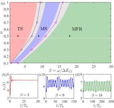
Figure 6: (a) Phase diagram for $L=12$ with ED ($U=0.8$, $N=5$). TS, MS and MFR correspond to thermalized state, mixing state and multifrequency resonance state, respectively. (b) - (d) There examples for these phases for $\alpha=0.5$ for the three symbols in (a). The grey regimes show the uncertainty of the phase boundaries.

Phase diagram. We finally address the phase diagram for the searching of the multifrequency resonance phase. From the above analysis the modulation frequency matters. This modulation frequency has a number of important consequences to the dynamics. In the extremely low modulation limit, the system follows adiabatically the dynamics of the Hamiltonian. In the high-frequency limit, that is, $\omega\gg\text{max}(\epsilon_{n})-\text{min}(\epsilon_{n})$, the effective dynamics can be well described by the effective Floquet Hamiltonian defined by $U(T_{0})=\exp(-iH_{\text{F}}T_{0})$ Blanes et al. (2009); Goldman and Dalibard (2014). To the third-order approximation Eckardt (2017); Eckardt and Anisimovas (2015), $H_{\text{F}}=-J_{\text{F}}\sum_{i}(b_{i}^{\dagger}b_{i+1}+h.c.)+\frac{U}{2}\sum_{i}n_{i}(n_{i}-1)$, where $J_{\text{F}}=(1-\frac{5\alpha^{2}}{12\omega^{2}})J$. The latter case was widely used in literature for the searching of novel phases, including the spin-orbit coupling Jackeli and Khaliullin (2009); Liu et al. (2011); Galitski and Spielman (2013) in lattice models as well as some exotic topological phases Liu et al. (2014); Neupane et al. (2014); Li and Sarma (2015). We are mainly interested in the physics between these two limits. In Fig. 6, we show that in the relatively low modulation limit, the wave function is thermalized. With the increasing of modulation frequency, it enters the mixed phase, which exhibits non-regular oscillation. From its Fourier spectroscopy, one may see multiply modulation frequencies due to the coupling of a lot of low-lying eigenstates. In this way, the period oscillation is hard to be developed in the experimental accessible time. With the further increase of modulation frequency, the dynamics will finally be restricted to the lowest two states, in which almost perfect oscillation can be found. The crossover between these three cases is somewhat smooth, probably due to the finite size effect. We also find the on-set of the multifrequency resonance depends strongly on the inclination $\alpha$. The larger this inclination is, the larger the commensurate ratio is required to be.

To conclude, we generalize the idea of multifrequency resonance from the single-particle physics to the many-body physics using a quantum seesaw based on an interacting Bose-Hubbard model. This phase is realized by commensurate between precession dynamics and nutation dynamics in the many-body system. In this model, the periodic driving field is used to restrict the dynamics of the wave function to the lowest two energy levels, which may also be realized in the other modulation systems. In this sense, this behavior should be quite general in a lot of periodic driving many-body systems before fully entering the effective Floquet Hamiltonian regime. This kind of dynamics is robust against non-integrability interactions.