Tensor non-Gaussianities from Non-minimal Coupling to the Inflaton

Abstract

Tensor non-Gaussianity represents an important future probe of the physics of inflation. Inspired by recent works, we elaborate further on the possibility of significant primordial tensor non-Gaussianities sourced by extra fields during inflation. Unitarity constraints limit the impact of extra (spinning) particle content by means of a lower bound on the corresponding mass spectrum. For spin-2 particles, this takes the form of the well-known Higuchi bound. Massive ($m\gtrsim H$) particles will typically decay during inflation unless they are non-minimally coupled to the inflaton sector: the inflating field “lifts” the dynamics of the extra field(s), effectively getting around the limits imposed by unitarity. There exist several models that realize such a mechanism, but we focus here on the set-up of [1] where, through an EFT approach, one is able to capture the essential features common to an entire class of theories. In the presence of an extra massive spin-2 particle, the interactions in the tensor sector mimic very closely those in the scalar sector of quasi-single-field inflationary models. We calculate the tensor bispectrum in different configurations and extract its dependence on the extra tensor sound speed. We show in detail how one may obtain significant tensor non-Gaussianities whose shape-function interpolates between local and equilateral, depending on the mass of the extra field. We also estimate the LISA response functions to a tensor bispectrum supporting the intermediate-type shapes we find.

1 Introduction

The existence of primordial gravitational waves is one of the key predictions of the inflationary paradigm [2, 3]. In the simplest scenarios inflation is driven by a single scalar field with canonical kinetic terms, and the corresponding predictions on the tensor power spectrum are that of a small almost scale-invariant signal, slightly decreasing towards smaller length scales. In these set-ups vacuum fluctuations are the leading source of the signal and the value of the Hubble parameter $H$ during inflation is the only unknown quantity: a detection would immediately reveal the energy scale of inflation. However, a growing literature [4, 5] of inflationary models points to the fact that predictions for primordial gravitational waves (PGW) can deviate dramatically from this simple picture. The crucial common ingredient is the presence of (a remnant of) extra degrees of freedom sourcing PGW.
Adding particle content to the inflationary Lagrangian can:

• break the one-to-one correspondence between $H$ and the energy scale of inflation;

• greatly enhance the amplitude of the tensor signal;

• violate consistency relations related to the squeezed limit of the tensor bispectrum;

• completely change the scale dependence of the power spectrum in favour of, for example, a blue spectrum or a localised (sometimes termed “bump”) feature.

The latter effect is particularly relevant in light of the possibility of detection at small scales via ground-based and space-based interferometers [6]. Indeed, whilst assuming a constant tilt of the primordial tensor power spectrum one may extrapolate from the ESA Planck mission results [7] (combined with LIGO and Virgo [8]) tight constraints on small scales, there is much more scope to accommodate and test a signal exhibiting features across different scales.
Of course one ought to strive to ask not just “what is possible” but also “what is natural or compelling” according to some agreed upon criterion. Let us briefly mention one example. Axions and axion-like particles are ubiquitous in physics, from QCD [9] to inflationary models [10]. In the latter context, the (approximate) shift symmetry of the axion potential is perhaps the most appealing property of such models: it makes it possible to tackle the so-called $\eta$-problem, i.e. the symmetry protects the inflaton mass under large quantum corrections [11]. Intriguingly, it tuns out that coupling an inflating axion to gauge fields during inflation is a way to make natural inflation [11] more natural [10]. These extra gauge fields are a dissipation channel for the (originally too steep) inflaton potential. Remarkably, they may also become the leading source for PGW, delivering a chiral gravitational wave spectrum with a bumpy profile at certain scales [12] and potentially large tensor non-Gaussianities peaking in the equilateral configuration. We stress that this class of models is by no means an exhaustive or sufficiently representative set of the many more existing mechanisms for PGW generation – see for example the recent [13] for a new mechanism for enhancing tensor modes at small scales, exploiting a non-attractor phase for single-field inflation. In general, we refer the interested reader to the review work in [14] for a more thorough survey of the literature.
In this work we shall embrace a rather different perspective on PGW generation. Instead of committing to a specific model, making a case for its naturalness in the model-building sense, and delivering its prediction, we will follow the general effective theory approach of [1]. Much in the spirit of earlier work [15], where an effective field theory of fluctuations around an inflating background was built for the single field case, the study in [1] extends this analysis to include extra fields with sizable coupling to the inflaton sector. The non-trivial nature of the coupling is of particular relevance given that we are after enhancing the PGW spectrum.
Extra scalars, vectors, tensors and higher-spin degrees of freedom have all been enlisted to generate gravitational waves. Unlike the case of scalars and (Abelian) vector fields, for which the sourcing typically occurs at non-linear order, starting with tensors one may feed the gravitational wave signal already at first order. The trouble is that, as one goes up the spin ladder, unitarity is increasingly demanding on the mass spectrum of the particle content [16, 17, 18], for which constraints of the form $m\gtrsim H$ are typically in place.
Quantum fluctuations associated to a particle in that mass range will inevitably decay during inflation unless a non-minimal coupling to the inflaton sector sustains them. The effective Lagrangian put forward in [1] includes the most general form a similar non-trivial coupling might take. In what follows, we will rely on the interactions, starting already at quadratic order, between the standard tensor sector and that of an additional spin-2 particle $\sigma$. Intriguingly, these are reminiscent of the dynamics characterising the scalar sector of quasi-single field inflation (QsF) [19]. Indeed, we recover many of the QsF features. The most relevant difference lies in the speed of propagation for the extra tensor (scalar) sector $\sigma$: bounds on tensor (scalar) non-Gaussianity, do (not) allow a small sound speed.
In this work we focus on the effects of the extra field content on the tensor sector. In particular, we examine tensor non-Gaussianities, an observable which can provide a useful probe of the inflationary particle zoo for a wide range of scales, ranging from the CMB, to large-scale structure, all the way to interferometers. We show that couplings with additional tensor fields can enhance the amplitude of tensor non-Gaussianities, and lead to new shapes for the tensor bispectrum.

The manuscript is organised as follows: in Section 2 we briefly review the EFT approach that provides the quadratic and cubic interactions at the basis of our bispectrum calculation; in Section 3 we show in detail the effect of an additional spin-2 particle on tensor non-Gaussianity, we derive the corresponding shape, its dependence on the mass of the extra field as well as its sound speed; in Section 3 we also undertake the first step towards producing forecasts for the capability of LISA to detect tensor non-Gaussianities in models such as the one under study, we do so by computing the response function for bispectrum shapes that are intermediate between the local and the equilateral; in Section 4 we discuss our findings, point out possible future directions and offer our conclusions; some of the details of our calculations can be found in the Appendix.

2 Brief Review of the Effective Framework

The original formulation of the effective field theory for inflation (EFTI) [15] provides a general Lagrangian starting from the realisation that the inflaton background breaks time-reparametrisation invariance. Full diffeomorphism (diff) invariance can be restored including the Goldstone mode $\pi$ that non-linearly realises time diffs. The result is a theory that describes scalar perturbations around FRW and covers a vast range of single-field inflationary models (see [22] for an extension of this approach).
There is a vast literature exploring the impact on cosmological observables resulting from adding extra ingredients to the single-field picture. The simplest next step is to add scalar degrees of freedom [23]. Perhaps even more interesting a phenomenology results from considering the presence of extra spinning particles. This often comes at a price: severe bounds on the mass range, affecting most dramatically particles of spin-2 and higher according to

$$s(s-1)\leq\frac{m^{2}}{H^{2}}<\left(s-\frac{1}{2}\right)^{2}\quad;\quad\frac{m^{2}}{H^{2}}\geq\left(s-\frac{1}{2}\right)^{2},$$ (2.1)

where the first expression corresponds to the principal series and the second one to the complementary series. We refer the reader to [24] and [18] where these conditions are explored at length in the inflationary context. It is also important to mention that interesting literature specifically dedicated to signatures of higher spin fields exists in [25]. The set of inequalities in Eq. (2.1) stems from the familiar identification of particles as unitary irreducible representation of the spacetime (de Sitter, in this case) isometry group [30]. The most immediate consequence of Eq. (2.1) on observables is that extra spinning particles are heavy and have little to no impact on late time correlation functions: they typically decay during inflation, can only appear as internal Feynman lines and theirs is a small integrated-over-time effect.
There is, however, a way to go around these limitations and boost the effect of extra spinning fields. The key step is to exploit the fact that inflationary dynamics breaks de Sitter isometries: the inflaton background spontaneously breaks the Lorentz group down to the rotation group. Coupling extra fields directly with the inflaton will then relieve them from the strict conditions in Eq. (2.1). Intuitively speaking, “non-minimal” coupling to the inflaton field provides sufficient mixing with the non-decaying inflaton mode to keep extra spinning particles afloat, effectively allowing them to be light.
The procedure to obtain the most general Lagrangian mimics the one in [15], with some important extra subtleties. The most immediate path stems from recognizing that fields should be identified as representations of the unbroken group (rotations): the Lagrangian one is after will then non-linearly realise the broken group. One starts with a field transforming in any tensor representation of the 3D rotation group and then embeds it in spacetime. For the case of a spin-2 particle, the resulting symmetric traceless tensor, propagating five degrees of freedom is embedded and coupled via [1]:

$$\Sigma^{00}=\frac{\partial_{i}\pi\partial_{j}\pi}{(1+\dot{\pi})^{2}}\Sigma^{ij}\quad;\quad\Sigma^{0j}=-\frac{\partial_{i}\pi}{(1+\dot{\pi})}\Sigma^{ij}\;,$$ (2.2)

where $\pi(t,{\bf x})$ is the usual inflaton fluctuation, related to the standard curvature perturbation $\zeta$ via $\zeta=-H\pi$, at leading order. Equipped with the building blocks outlined above, and combining those with the usual ones from the EFTI, the authors of [1] arrive at what will be our starting point: the quadratic and cubic inflationary Lagrangian including interactions between standard metric tensors fluctuations $\gamma_{ij}$ with those from a generic extra spin-2 field $\sigma_{ij}$, as well as self-interactions of $\sigma_{ij}$ itself :

$$\mathcal{L}_{\gamma+\sigma}=\mathcal{L}^{(2)}_{\text{free}}+\mathcal{L}^{(2)}_{\text{int}}+\mathcal{L}^{(3)}_{\text{int}}\,,$$ (2.3)

where

$$\mathcal{L}^{(2)}_{\text{free}}=\frac{a^{3}}{8}\left[\left(\dot{\tilde{\gamma}}_{ij}\right)^{2}-\frac{1}{a^{2}}\left(\partial_{i}{\tilde{\gamma}}_{jk}\right)^{2}\right]+\frac{a^{3}}{4}\left[\left(\dot{\sigma}_{ij}\right)^{2}-\frac{c_{\sigma}^{2}}{a^{2}}\left(\partial_{i}\sigma_{jk}\right)^{2}-m_{\sigma}^{2}\left(\sigma_{ij}\right)^{2}\right]\,,$$ (2.4)

$$\mathcal{L}^{(2)}_{\text{int}}=\frac{a^{3}}{2}\,\rho\,\sigma^{ij}\dot{\tilde{\gamma}}_{ij}\,,\quad\quad\quad\mathcal{L}^{(3)}_{\text{int}}=-a^{3}\,\mu\left(\sigma_{ij}\right)^{3}\,,$$ (2.5)

with $c_{\sigma}$ the sound speed for the helicity-2 component of the extra spin-2 field. Note that we have canonically normalized metric fluctuations according to $\tilde{\gamma}_{ij}\equiv M_{\rm Pl}\gamma_{ij}$, where $\gamma_{ij}$ is the standard dimensionless metric perturbation. We will return to dimensionless quantities in Eq. (3.2). We take a sound speed equal to one for the tensor perturbations of the metric and $m_{\sigma}$ stands for the mass of the extra spin-2 field. The mass range of interest for us will be that corresponding to $0\leq\nu\lesssim 1$, with $\nu=\sqrt{9/4-m_{\sigma}^{2}/H^{2}}$, which corresponds to interesting phenomenology for tensor non-Gaussianities and interpolates, as we shall see, between different shape profiles.
The quadratic mixing and cubic self-interaction in (2.5) are the building blocks necessary to compute the diagram in Fig. 1.

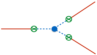
Figure 1: Diagrammatic representation of the contribution of $\sigma$ to the bispectrum of gravitational waves. Red/solid lines indicate propagators of $\gamma$, blue/dotted lines of $\sigma$. The blue vertex indicates the interaction given in $\mathcal{L}^{(3)}_{\text{int}}$, the green vertices correspond to the one from $\mathcal{L}^{(2)}_{\text{int}}$ (Eq. (2.5)).

It is worth pointing out two notions at this stage:
– the approach we are adopting here is a fully-fledged effective theory one, this is not akin to employing a specific parametrisation of fluctuations around FRW because here all operators compatible with the symmetries of the theory are automatically included;
– the couplings to the inflaton fluctuations obtained via the construction in [1] are not arbitrary, they emerge from the fact that de Sitter isometries are non-linearly realised.

3 Tensor bispectrum

In this section we compute the tensor bispectrum mediated by the additional spin-2 field. Let us first report the solutions for the mode functions and for the tensor power spectrum. The tensor components of the spin-2 fields are expanded as

$$T_{ij}(\textbf{x},\tau)=\int\frac{d^{3}k}{(2\pi)^{3}}\,e^{i\textbf{k}\cdot\textbf{x}}\,\sum_{\lambda}\epsilon^{\lambda}_{ij}(\hat{k})T^{\lambda}_{\textbf{k}}(\tau)\,,$$ (3.1)

where $T$ is a place holder for $\gamma$ and $\sigma$. In what turns out to be a very convenient simplification, note that, upon requiring $\rho/H\ll 1$, the mixing term $\mathcal{L}^{(2)}_{\text{int}}$ can be treated as a perturbation on top of $\mathcal{L}^{(2)}_{\text{free}}$. The very same $\rho/H$ ratio appears in late-time observables, starting with the tensor power spectrum. Similarly, we require $\mu/H\ll 1$ for $\mathcal{L}^{(3)}_{\text{int}}$ to be treated as a perturbation. The mode-functions for $\sigma$ and $\gamma$ are then the solutions to the free-field equations

$$\gamma_{k}(\tau)=\frac{2iH}{M_{\text{Pl}}\sqrt{2k^{3}}}\left(1+ik\tau\right)e^{-ik\tau}\,,$$ (3.2)

$$\sigma_{k}(\tau)=\sqrt{\frac{\pi}{2}}H\left(-\tau\right)^{3/2}\,\mathcal{H}^{(1)}_{\nu}[-c_{\sigma}k\tau]\,,$$ (3.3)

where $\nu\equiv\sqrt{9/4-(m_{\sigma}^{2}/H^{2})}$ and $\mathcal{H}^{(1)}_{\nu}$ is the Hankel function of the first kind. The power spectrum of gravitational waves receives a contribution from the mixing with the extra spin-2 field

$$P_{\gamma}(k)=\frac{4H^{2}}{M_{\text{Pl}}^{2}\,k^{3}}\left[1+\frac{\mathcal{C}_{\gamma}(\nu)}{c_{\sigma}^{2\nu}}\left(\frac{\rho}{H}\right)^{2}\right]\equiv\frac{4H^{2}}{M_{\text{Pl}}^{2}\,k^{3}}\left[1+\alpha_{\gamma}\right]\,,$$ (3.4)

where the function $C_{\gamma}(\nu)$ can be found in [1] and applies to the case of finite mass for $\sigma$. The quantity $C_{\gamma}(\nu)$ encapsulates the effect of the quadratic $\gamma-\sigma$ interaction on the tensor power spectrum. We stress here that, for the $\nu$ range of interest, this quantity as well as its scalar sector counterpart $\mathcal{C}_{\zeta}(\nu)$ in Eq. (3.16) are of order one to ten.

Upon using the parametrization for the power spectrum in the RHS of Eq. (3.4), one finds for the tilt

$$n_{T}=-2\epsilon+\frac{\dot{\alpha}_{\gamma}}{H(1+\alpha_{\gamma})}\,.$$ (3.5)

One therefore needs to allow for a time dependence in $c_{\sigma}$ or $\rho$ in order to support a blue tensor spectrum . We do not expect a time-dependent sound speed to qualitatively change, for example, the shape-function profile of non-Gaussianities and it is also with this in mind that we will provide in Section 3.3 our results for the LISA response function for a bispectrum momentum dependence that, as is the case for the model under consideration, interpolates between the local and the equilateral shapes (see Section 3.2). Naturally, one may look for a large primordial tensor signal already at CMB scales. Planned future probes, such as the LiteBIRD satellite, will measure polarization anisotropies over the full sky. LiteBIRD will constrain the tensor to scalar ratio down to $\Delta r=0.001$ and improve the constraints on $f^{\rm tensor}_{\rm nl}$ [31]. CMB-S4 experiments [32] will also deliver substantial improvements on current bounds.

We now move on to presenting our results for the contribution to the gravitational waves bispectrum represented by the diagram in Fig. (1), and refer the reader to Appendix A for further related details. The $\sigma$-mediated contribution reads

$$\langle\gamma^{\lambda_{1}}_{\textbf{k}_{1}}\gamma^{\lambda_{2}}_{\textbf{k}_{2}}\gamma^{\lambda_{3}}_{\textbf{k}_{3}}\rangle_{(\sigma)} = (2\pi)^{3}\delta^{(3)}(\textbf{k}_{1}+\textbf{k}_{2}+\textbf{k}_{3})\mathcal{A}^{\lambda_{1}\lambda_{2}\lambda_{3}}\,B_{(\sigma)}(k_{1},k_{2},k_{3})\,,$$ (3.6)

where

$$\mathcal{A}^{\lambda_{1}\lambda_{2}\lambda_{3}}\equiv\epsilon^{\lambda_{1}}_{\alpha\beta}(-\hat{k}_{1})\epsilon^{\lambda_{2}}_{\beta\gamma}(-\hat{k}_{2})\epsilon^{\lambda_{3}}_{\gamma\alpha}(-\hat{k}_{3})\;,$$ (3.7)

and

$$B_{(\sigma)}(k_{1},k_{2},k_{3}) = \frac{12\pi^{3}}{k_{1}^{4}k_{2}k_{3}}\frac{\mu}{H}\frac{\rho^{3}}{M_{\text{Pl}}^{3}}\mathcal{F}_{\nu c_{\sigma}}(k_{1},k_{2},k_{3})+\text{5\,perms}\,.$$ (3.8)

Here $\mathcal{F}_{\nu c_{\sigma}}$ is a lengthy function of the momenta and it depends on the parameters $\nu$ and $c_{\sigma}$, see Eqs. (A)-(A). It is important to point out that the tensor bispectrum, unlike its scalar counterpart, also depends on the orientation of the 3-momentum vectors $\bm{\mathrm{{k}}}_{i}$, and not merely on their norm. As a result, when performing calculations it will be necessary to choose a reference orientation for the $k_{i}$ triangle sides. For simplicity, we avoid including the explicit dependence on the directions in $B_{(\sigma)}$ and express it only in terms of the size $k_{i}$ of the three momenta. Also, we point out that the bispectrum dependence on chirality has been extracted in the overall factor $\mathcal{A}^{\lambda_{1}\lambda_{2}\lambda_{3}}$, and there is no intrinsic chirality dependence in the bispectrum $B_{(\sigma)}\,$.

3.1 Amplitude

As can be anticipated by means of the analogy with the QsF case, the contributions to the tensor bispectrum we are after will lead to a non-zero amplitude both in the equilateral ($k_{1}\sim k_{2}\sim k_{3}$) and in the squeezed limit ($k_{3}\ll k_{2}\sim k_{3}$) for most values of the mass $m_{\sigma}$. We find it useful then to provide below the complete expressions for the bispectrum (3.8) in the squeezed and equilateral configurations

$$B_{(\sigma)}(k_{1},k_{2},k_{3})|_{k_{1}\sim k_{2}\gg k_{3}}\simeq\frac{3\pi^{2}\cdot 2^{3+\nu}}{k_{1}^{7/2-\nu}k_{2}\,k_{3}^{3/2+\nu}}\,\frac{\mu}{H}\frac{\rho^{3}}{M_{\text{Pl}}^{3}}\,s^{\text{sq}}(\nu,c_{\sigma})\,,$$ (3.9)

$$B_{(\sigma)}(k_{1},k_{2},k_{3})|_{k_{1}\sim k_{2}\sim k_{3}}=\frac{9\pi^{3}\cdot 2^{3}}{k_{1}^{6}}\frac{\mu}{H}\frac{\rho^{3}}{M_{\text{Pl}}^{3}}\,s^{\text{eq}}(\nu,c_{\sigma})\,,$$ (3.10)

where

$$s^{\text{sq}}(\nu,c_{\sigma}) \equiv \frac{\Gamma[\nu]}{c_{\sigma}^{\nu}}\int_{-\infty}^{0}dx_{1}\int_{-\infty}^{x_{1}}dx_{2}\int_{-\infty}^{x_{2}}dx_{3}\Big{\{}(-x_{1})^{-1/2}(-x_{2})^{1/2-\nu}(-x_{3})^{-1/2}\sin(-x_{1})$$ (3.11)

$$\times\text{Im}\left[\mathcal{H}_{\nu}^{(1)}(-c_{\sigma}x_{1})\mathcal{H}_{\nu}^{(2)}(-c_{\sigma}x_{2})\right]\text{Im}\left[\mathcal{H}_{\nu}^{(1)}(-c_{\sigma}x_{2})\mathcal{H}_{\nu}^{(2)}(-c_{\sigma}x_{3})\,e^{ix_{3}}\right]$$

$$+(-x_{1})^{-1/2}(-x_{2})^{-1/2}(-x_{3})^{1/2-\nu}\sin(-x_{1})\sin(-x_{2})$$

$$\times\text{Im}\left[\mathcal{H}_{\nu}^{(2)}(-c_{\sigma}x_{1})\mathcal{H}_{\nu}^{(2)}(-c_{\sigma}x_{2})\left(\mathcal{H}_{\nu}^{(1)}(-c_{\sigma}x_{3})\right)^{2}\right]$$

$$\times\int_{-\infty}^{0}dy_{4}(-y_{4})^{-1/2}\text{Re}\left[\mathcal{H}_{\nu}^{(1)}(-c_{\sigma}y_{4})\,e^{-iy_{4}}\right]\Big{\}}\,,$$

and

$$s^{\text{eq}}(\nu,c_{\sigma}) \equiv \int_{-\infty}^{0}dx_{1}\int_{-\infty}^{x_{1}}dx_{2}\int_{-\infty}^{x_{2}}dx_{3}\int_{-\infty}^{x_{3}}dx_{4}\Big{\{}\sqrt{\frac{x_{2}}{x_{1}x_{3}x_{4}}}\text{Im}\left[\mathcal{H}_{\nu}^{(1)}(-c_{\sigma}x_{1})\mathcal{H}_{\nu}^{(2)}(-c_{\sigma}x_{2})\right]$$ (3.12)

$$\times\text{Im}\left[\mathcal{H}_{\nu}^{(2)}(-c_{\sigma}x_{2})\mathcal{H}_{\nu}^{(1)}(-c_{\sigma}x_{4})\,e^{-ix_{4}}\right]\text{Im}\left[\mathcal{H}_{\nu}^{(1)}(-c_{\sigma}x_{2})\mathcal{H}_{\nu}^{(2)}(-c_{\sigma}x_{3})\,e^{ix_{3}}\right]\sin(-x_{1})$$

$$+\sqrt{\frac{x_{3}}{x_{1}x_{2}x_{4}}}\sin(-x_{1})\sin(-x_{2})\text{Im}\left[\mathcal{H}_{\nu}^{(2)}(-c_{\sigma}x_{1})\mathcal{H}_{\nu}^{(2)}(-c_{\sigma}x_{2})\left(\mathcal{H}_{\nu}^{(1)}(-c_{\sigma}x_{3})\right)^{2}\right]$$

$$\times\text{Im}\left[\mathcal{H}_{\nu}^{(2)}(-c_{\sigma}x_{3})\mathcal{H}_{\nu}^{(1)}(-c_{\sigma}x_{4})\,e^{-ix_{4}}\right]+\sqrt{\frac{x_{4}}{x_{1}x_{2}x_{3}}}\sin(-x_{1})\sin(-x_{2})\sin(-x_{3})$$

$$\times\text{Im}\left[\left(\mathcal{H}_{\nu}^{(1)}(-c_{\sigma}x_{4})\right)^{3}\mathcal{H}_{\nu}^{(2)}(-c_{\sigma}x_{1})\mathcal{H}_{\nu}^{(2)}(-c_{\sigma}x_{2})\mathcal{H}_{\nu}^{(2)}(-c_{\sigma}x_{3})\right]\Big{\}}\,.$$

Let us now compute the bispectrum amplitude, $f_{\text{nl}}$, which we define as

$$B_{(\sigma)}(k_{1},k_{2},k_{3})=f_{\text{nl}}\,\left(\frac{H^{2}}{4\epsilon\,M_{\text{Pl}}^{2}}\right)^{2}\,F(k_{1},k_{2},k_{3})\,,$$ (3.13)

where (from Eqs. (3.9), (3.10)):

$$F(k_{1},k_{2},k_{3})=\begin{cases}\frac{1}{k_{1}^{6}},&\,\,\text{for $k_{1}\sim k_{2}\sim k_{3}$}.\\ \frac{1}{k_{1}^{9/2-\nu}\,k_{3}^{3/2+\nu}},&\,\,\text{for $k_{1}\sim k_{2}\gg k_{3}$}.\end{cases}$$ (3.14)

We will compute the bispectrum amplitudes for $\nu=1$. We choose this particular value because we find it particularly instructive in that the corresponding shape-function exhibits a non-zero component both in the local and equilateral configurations. It is well-known that, upon employing massive fields, one may indeed interpolate between these two standard templates. We shall see this more explicitly in Section 3.2.

We report in Fig. (2) our numerical results for the functional behaviour of $s^{\text{sq}}(c_{\sigma},\nu)$ and $s^{\text{eq}}(c_{\sigma},\nu)$ for $\nu=1$, which are consistent with the power laws

$$s^{\text{sq}}(1,c_{\sigma})\simeq\frac{7.4}{c_{\sigma}^{4.06}}\,,\quad\quad s^{\text{eq}}(1,c_{\sigma})\simeq\frac{2.5}{c_{\sigma}^{4.05}}\,.$$ (3.15)

Figs. (3) and (4) show the behaviour of, respectively, $s^{\text{sq}}$ and $s^{\text{eq}}$, as a function of $\nu$ for fixed values of the sound speed. For $c_{\sigma}=1$ our numerical results are in agreement with the calculations in the scalar sector of QsF inflation [19].

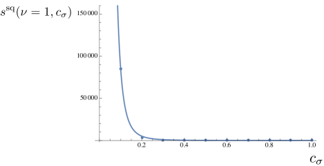
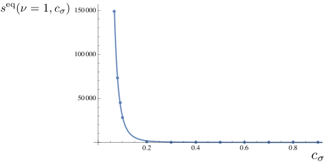
Figure 2: (Left panel) Plot of numerical values of the coefficient $s^{\text{sq}}(\nu,c_{\sigma})$ defined in Eq. (3.11), as a function of $c_{\sigma}$ and for $\nu=1$. The solid line corresponds to the fit in Eqs. (3.15). (Right panel) Numerical values for $s^{\text{eq}}(\nu,c_{\sigma})$ (Eq. (3.12)) as a function of the sound speed for $\nu=1$, with the solid line representing the functional dependence in Eq. (3.15).

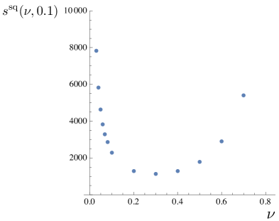
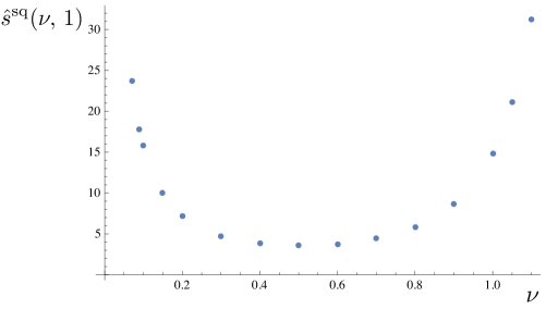
Figure 3: (Left panel) Numerical values of $s^{\text{sq}}(\nu,c_{\sigma})$ for fixed $c_{\sigma}=0.1$. (Right panel) Numerical values of $\hat{s}^{\text{sq}}(\nu,c_{\sigma})\equiv(3\pi^{2}/2^{3-\nu})\,s^{\text{sq}}(\nu,c_{\sigma})$ for $c_{\sigma}=1$. Here we rescaled the coefficient $s^{\text{sq}}(\nu,c_{\sigma})$ for the sake of comparison with [19] (see Fig. 9 therein).

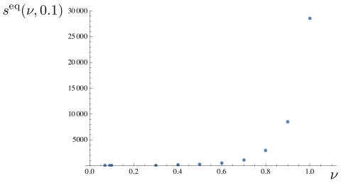
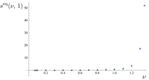
Figure 4: (Left panel) Numerical values of $s^{\text{eq}}(\nu,c_{\sigma})$ for fixed $c_{\sigma}=0.1$. (Right panel) Numerical values of $s^{\text{eq}}(\nu,c_{\sigma})$ for fixed $c_{\sigma}=1$.

The scalar power spectrum is given by [1]

$$P_{\zeta}(k)=\frac{H^{2}}{4\epsilon M_{\text{Pl}}^{2}\,k^{3}}\left[1+\frac{\mathcal{C}_{\zeta}(\nu)}{\epsilon\,c_{0}^{2\nu}}\left(\frac{\rho}{H}\right)^{2}\right]\equiv\frac{H^{2}}{4\epsilon M_{\text{Pl}}^{2}\,k^{3}}\left[1+\alpha_{\zeta}\right]\,,$$ (3.16)

where $c_{0}$ is the sound speed for the helicity zero component of $\sigma$. The condition $\rho\ll c_{0}\sqrt{\epsilon}H$ ensures that radiative corrections to $m_{\sigma}$ remain small [1]. For values of $\nu$ in the vicinity of 1, this implies $\alpha_{\zeta}\ll 1$ and therefore a scalar power spectrum dominated by vacuum fluctuations, $P_{\zeta}\simeq H^{2}/(4\epsilon M_{\text{Pl}}^{2}k^{3})$. On the other hand, the tensor power spectrum, (3.4), may be dominated either by the sourced or by the vacuum contributions (or the two may be comparable to one another) depending on parameters choice. One can therefore employ the following relation in Eq. (3.13): $H^{2}/(4\epsilon\,M_{\text{Pl}}^{2})=(1/r)\cdot(1+\alpha_{\gamma})\,4\,H^{2}/M_{\text{Pl}}^{2}\;$, where the tensor to scalar ration $r$ is defined as usual by $r\equiv\mathcal{P}_{\gamma}/\mathcal{P}_{\zeta}$ .
Let us consider the equilateral limit first. Using Eqs. (3.10) and (3.15), the definition in (3.13) gives

$$f_{\text{nl}}^{\text{eq}}\simeq r^{2}\cdot\left(\frac{2.5\cdot 9\cdot\pi^{3}}{2}\right)\left(\frac{\mu}{H}\right)\left(\frac{\rho}{H}\right)^{3}\left(\frac{M_{\text{Pl}}}{H}\right)\frac{1}{c_{\sigma}^{4}\,(1+\alpha_{\gamma})^{2}}\,,$$ (3.17)

Let us analyze the three cases: $\alpha_{\gamma}\ll 1$, $\alpha_{\gamma}\gg 1$ and $\alpha_{\gamma}\simeq 1$, using the relation $M_{\text{Pl}}\sqrt{\epsilon}/H\simeq 10^{3}$ (from the amplitude of the scalar power spectrum), together with $r=16\,\epsilon\,(1+\alpha_{\gamma})$ (from the definition of tensor-to-scalar ratio combined with Eq. (3.4)). From (3.4) and for $\nu=1$ one also finds: $\alpha_{\gamma}(1+\alpha_{\gamma})=(10/16)(r/c_{\sigma}^{2})(\rho/(\sqrt{\epsilon}H))^{2}$. These relations are to be combined with the constraints $\rho/(\sqrt{\epsilon}H)\ll 1$ and $\mu/H\ll 1$ .
Equation (3.17) can be rewritten as

$$f_{\text{nl}}^{\text{eq}}\simeq\left[4.4\times 10^{4}\left(\frac{\mu}{H}\right)\left(\frac{1}{c_{\sigma}}\right)\left(\frac{1}{r^{1/2}}\right)\left(\frac{\alpha_{\gamma}}{1+\alpha_{\gamma}}\right)^{3/2}\right]r^{2}\,.$$ (3.18)

As an example, a tensor-to-scalar ratio near the current bound of $0.06$ [7] and a value of $\mu/H=0.5$ would yield:

$(i)$ $\alpha_{\gamma}=\mathcal{O}(10^{-1})$:

$$f_{\text{nl}}^{\text{eq}}\simeq\begin{cases}\frac{6957}{\sqrt{r}}\,r^{2}\simeq 102&\,\,\text{for $c_{\sigma}=0.1$}\,;\\ \frac{12060}{\sqrt{r}}\,r^{2}\simeq 177,&\,\,\text{for $c_{\sigma}=0.05$}\,;\\ \frac{60302}{\sqrt{r}}\,r^{2}\simeq 886&\,\,\text{for $c_{\sigma}=0.01$}\,.\end{cases}$$ (3.19)

$(ii)$ $\alpha_{\gamma}=\mathcal{O}(1)$:

$$f_{\text{nl}}^{\text{eq}}\simeq\begin{cases}\frac{77782}{\sqrt{r}}\,r^{2}\simeq 1143&\,\,\text{for $c_{\sigma}=0.1$}\,;\\ \frac{155563}{\sqrt{r}}\,r^{2}\simeq 2286,&\,\,\text{for $c_{\sigma}=0.05$}\\ \frac{777817}{\sqrt{r}}\,r^{2}\simeq 11431&\,\,\text{for $c_{\sigma}=0.01$}\,.\end{cases}$$ (3.20)

$(iii)$ $\alpha_{\gamma}=\mathcal{O}(10)$: in this case, only values $c_{\sigma}<0.02$ are compatible with the above conditions on the parameter space

$$f_{\text{nl}}^{\text{eq}}\simeq\frac{2\cdot 10^{6}}{\sqrt{r}}\,r^{2}\simeq 28026\quad\text{for \; $c_{\sigma}=0.01$}\;.$$ (3.21)

Using Eqs. (3.9), (3.15), and (3.13), one finds slightly smaller values for the amplitude in the squeezed limit

$$f_{\text{nl}}^{\text{sq}}\simeq 0.6\,f_{\text{nl}}^{\text{eq}}\,.$$ (3.22)

These values of the amplitude can be compared with those due to bispectrum contributions from self-interactions of $\gamma$, which are also the only ones present in the minimal single-field inflationary models. One finds, for example [37, 38] (see e.g. also [39]):

$$f_{\text{nl},\text{standard}}^{\lambda_{1}\lambda_{2}\lambda_{3}(\text{eq})}\simeq\begin{cases}0.9\,r^{2},&\,\,\text{for $\,\,\lambda_{1}\lambda_{2}\lambda_{3}=RRR,\,LLL$}\,,\\ 0.01\,r^{2},&\,\,\text{for $\,\,\lambda_{1}\lambda_{2}\lambda_{3}=RRL,\,LLR$}\,,\end{cases}$$ (3.23)

$$f_{\text{nl},\text{standard}}^{\lambda_{1}\lambda_{2}\lambda_{3}(\text{sq})}\simeq 0.2\,r^{2},\quad\quad\,\,\,\text{for $\,\,\lambda_{1}\lambda_{2}\lambda_{3}=RRR,\,LLL,\,RRL,\,LLR\,,$}$$ (3.24)

for $\alpha_{\gamma}\leq 1$. For $\alpha_{\gamma}\gg 1$ the amplitudes in Eqs. (3.23)-(3.24) are suppressed by a factor $\sim\alpha_{\gamma}^{-2}$. Notice that in (3.23)-(3.24) we redefined the amplitude of the bispectrum to include the information on polarization. In other words, the amplitudes in (3.23)-(3.24) are to be compared with $f_{\text{nl}}^{\lambda_{1}\lambda_{2}\lambda_{3}(\text{eq/sq})}\equiv\mathcal{A}^{\lambda_{1}\lambda_{2}\lambda_{3}}f_{\text{nl}}^{(\text{eq/sq})}$ where, from its definition in Eq. (3.7) (see also (A.8)) one finds the following values for $\mathcal{A}^{\lambda_{1}\lambda_{2}\lambda_{3}}$:

	Squeezed limit ($k_{1}\sim k_{2}\gg k_{3}$)	Equilateral limit ($k_{1}\sim k_{2}\sim k_{3}$)
RRR, LLL	1/4	27/64
RRL, LLR	1/4	3/64
LRR, RLL, RLR, LRL	$(1/16)\cdot(k_{3}^{2}/k_{2}^{2})$	3/64

Table 1: Values of the function $\mathcal{A}^{\lambda_{1}\lambda_{2}\lambda_{3}}$ for various helicities combinations.

We have found that $c_{\sigma}$ values smaller than unity lead to an amplitude for the bispectrum sourced by the extra spin-2 field that can be several orders of magnitude larger than the one predicted in standard single-field slow-roll inflation.

3.2 Shape-Function

We now move on to study the dependence of the tensor bispectrum on the $(k_{1},k_{2},k_{3})$ configuration. The observable is a function of the norm of the wavenumbers and one can set, without loss of generality, the norm of one such wavenumber to one. Momentum conservation dictates that the three external momenta of the bispectrum form a closed triangle and, depending on the configuration probed, one refers to e.g. the aforementioned equilateral and squeezed cases. In analogy with the scalar QsF case, we expect our bispectrum to peak (whilst still exhibiting a non-zero value in the equilateral region) in the squeezed limit for $\nu\gtrsim 1$ and to display a plateau like profile for smaller value of $\nu$, flowing towards an equilateral-like shape in the vicinity of $\nu=0$. Intuitively, the close similarities with the scalar QsF sector are down to the fact that a $c_{\sigma}\ll 1$ (which is where we differ, given that $c^{\rm QsF}_{\sigma}=1$) affects equally all of the wavefunctions $(k_{1},k_{2},k_{3})$-dependence in the bispectrum calculation. The biggest impact of a small sound speed is then on the overall amplitude, not the shape profile.
Even before the actual calculation, and without the comparison with results from QsF, our findings are consistent with the following line of reasoning.
In the presence of only light fields and their (self)interactions, the peak configuration of the bispectrum can be extracted from identifying the type of interactions corresponding to each contribution: non-derivative interactions lead to a peak in the local configuration whilst increasing the number of derivative operators moves the profile towards equilateral or similar (e.g. orthogonal) shapes. Derivative interactions may indeed introduce powers of $k_{L}/k_{S}$ that disfavour the squeezed configuration. There is something to be added to this picture in the presence of massive states. Indeed, as pointed out elsewhere (see e.g.[35]), the additional $(k\tau)^{3/2-\nu}$ late-time behaviour of massive wave-functions effectively adds a $(k_{L}/k_{S})^{f(3/2-\nu)}$ in front of correlations functions and this has an effect on the overall shape that mimics the one due to the presence of derivative (self)interactions.

A few comments are in order about the conventions used in plotting the shape-functions. First of all, we note that in all the plots a multiplying factor of $(k_{1}k_{2}k_{3})^{2}$ has been included in front of the expression for the bispectrum to conform to the standard definition of shape, see e.g. [36]. Inspection of the RHS of Eq.(3.6) reveals the presence of the momentum-conservation delta function, the quantity $B_{(\sigma)}$, and also the factor $\mathcal{A}^{\lambda_{1}\lambda_{2}\lambda_{3}}$ which encapsulates the effect of tensor helicities. In order to facilitate the comparison with the scalar sector of QsF, we will not be including the effect of $\mathcal{A}^{\lambda_{1}\lambda_{2}\lambda_{3}}$ in the shape-function plots. It is worth mentioning that for most combinations of the helicities this factor would, if included, have no qualitative influence on the profile, the exception being the squeezed configuration of the combinations in the third row of Table (1). We also stress that the expression in Eq.(3.7) is different from the one characterising standard contributions (i.e. those not mediated by $\sigma$) to tensor non-Gaussianities and this fact may be used to distinguish the two scenarios.

We start with Fig. (5), where we plot the shape-function obtained numerically from the general expression in Eq.(3.8) for the case $c_{\sigma}=1/10,\,\nu=0$. The profile that emerges is one with a plateau that quickly and smoothly decreases towards much smaller values in the squeezed region. The shape has been normalised according to its numerical value in the equilateral point of the $(k_{2},k_{3})$ plane.

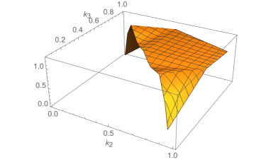
Figure 5: Plot of the numerically obtained shape-function $(k_{1}k_{2}k_{3})^{2}B_{\sigma}(k_{1},k_{2},k_{3},c_{\sigma},\nu)$ for $\nu=0,\,c_{\sigma}=1/10$ and where, without loss of generality, we have set $k_{1}=1$. The value $\nu=0$ corresponds to $m=3/2\,H$.

A rather different shape-function corresponds to the $\nu=1$ case: we are flowing towards smaller values of the mass for the $\sigma$ field in parameter space so that the plot in Fig. (6) exhibits a clear peak in the squeezed limit. Irrespective of the results on the numerical integrals derived from Eq.(3.8), we can extract analytically the $\nu$-dependent behaviour of the momenta in the squeezed limit. It reads:

$$B_{\sigma}(k_{1},k_{2},k_{3},\nu)\Big{|}_{k_{3}\ll k_{2}\sim k_{1}}\propto\left(\frac{1}{k_{1}^{7/2-\nu}\,k_{2}\,k_{3}^{3/2+\nu}}\;+\text{perms.}\right)\;,$$ (3.25)

where we have omitted any dependence on the overall amplitude as well as on the function $s^{\text{sq}}(\nu,c_{\sigma})$.

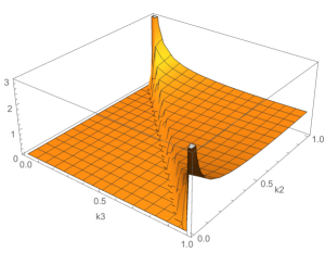
Figure 6: Plot corresponding to the shape-function $(k_{1}k_{2}k_{3})^{2}B_{\sigma}(k_{1},k_{2},k_{3},c_{\sigma},\nu)\Theta_{\rm Heav.}(k_{2}+k_{3}-1)$ for $\nu=1,\,c_{\sigma}=1/10$ and where, without loss of generality, we have set $k_{1}=1$. The value $\nu=1$ corresponds to $m\simeq 1.12\,H$. The shape-function has been obtained by extrapolating to the full $(k_{2},k_{3})$ plane our squeezed limit findings.

Strictly speaking, Eq. (3.25) describes very accurately the shape-function in two small regions centered on the $(0,1)$ and $(1,0)$ corners of the $(k_{2},k_{3})$ plane, but does not necessarily perform as well on the full plane. However, we have verified that, for the $\nu=1$ case, the shape obtained by extending the domain of Eq. (3.25) is indeed a good approximation for the full numerical result and it is the former that we plot in Fig. (6).
It is worth mentioning at this stage the tensor bispectrum shape-function corresponding to other, specific, models with extra particle content. A case in point is the tensor sector of the axion-gauge field model in [46]. Non-Gaussianities were analyzed for the first time in [47], followed by an even more detailed study [48] by the same authors. The resulting bispectrum is peaked in the equilateral limit but, rather interestingly, it also displays a very distinct behaviour in other regions of the $(k_{2},k_{3})$ plane. This (class of) model(s) is of course different from the set-up under scrutiny here. The most immediately identifiable difference at the level of observables is the possibility of a peak in the squeezed configuration, as illustrated in Fig. (6). We intuitively explain this by the fact that the most intruiging parameter space region of the model analysed in [47, 48] corresponds to a larger effective mass for the extra fields than the one we are probing here for $\nu\gtrsim 1$.

3.3 On LISA response functions for tensor bispectra with intermediate shapes

In the previous Sections, we learned that our scenario based on the EFT analysis of [1] can lead to many possibilities for the momentum dependence corresponding to the shape of the tensor bispectrum. Bispectra can interpolate between squeezed and equilateral configurations, depending on the values of parameters involved, and also other shapes are in principle possible. It is interesting to start asking what are the experimental prospects for distinguishing the shape and chirality dependence of the tensor bispectrum, in case of future detection of primordial gravitational waves from inflation. A systematic study of this problem by means of CMB polarisation is (as far as we are aware) still lacking, although a detailed investigation to analyse parity violating tensor bispectra maximised in equilateral configurations has been carried on by the Planck collaboration [34], based on templates developed in [40].

In this section we start exploring how interferometers can be sensitive to the shape of tensor bispectrum, focussing on LISA [41]. As explained in the Introduction, there are examples of inflationary scenarios with enhanced (w.r.t. the minimal case) amplitude of tensor power spectra and bispectra at interferometer scales. In case of direct couplings with additional spin two fields – as in the EFT framework we are examining – these scenarios can lead to new intermediate shapes for primordial tensor bispectra. The possibility of studying primordial tensor bispectra with LISA has been first investigated in [42], where the amplitude of the three-point function for time delays of photons travelling along the interferometer arms is connected, by means of the interferometer response function, with the amplitude and momentum dependence of primordial tensor bispectra. The starting equation is

$$\langle\Sigma^{3}(t)\rangle\,=\,\left(2\pi L\right)^{3}\,\sum_{\lambda_{1}\lambda_{2}\lambda_{3}}\int_{0}^{\infty}\prod_{i=1,2,3}k_{i}dk_{i}\,{\cal B}_{\lambda_{1}\lambda_{2}\lambda_{3}}(\hat{k}_{i}^{*},k_{i})\,\,{\cal R}_{\lambda_{1}\lambda_{2}\lambda_{3}}(\hat{k}_{i}^{*},k_{i})\,.$$ (3.26)

In the previous equation $\Sigma(t)$ is the time delay for a photon travelling along one of the channels of LISA interferometer . $L$ is the length of the interferometer arm. ${\cal B}_{\lambda_{1}\lambda_{2}\lambda_{3}}(\hat{k}_{i}^{*},k_{i})$ is the tensor bispectrum including the helicity indexes (in our specific case, it reads ${\cal B}_{\lambda_{1}\lambda_{2}\lambda_{3}}\,=\,{\cal A}_{\lambda_{1}\lambda_{2}\lambda_{3}}B_{(\sigma)}$ where the latter quantities are defined in Eqs. (3.7), (3.8)). ${\cal R}_{\lambda_{1}\lambda_{2}\lambda_{3}}(\hat{k}_{i}^{*},k_{i})$ is the interferometer three-point response function. The latter function depends on the size of three momenta, but also on the orientation of a reference choice of three-vectors. See [42] for full details on Eq. (3.26) and on how to calculate the three-point response function.

Ref. [42] analysed in full detail the momentum dependence of the interferometer response function focussing on the case of primordial tensor bispectra maximised in the equilateral or in the squeezed configurations. In this Section, we explore for the first time the detector response function to more general shapes of tensor bispectra. The shapes of tensor bispectra can be described in terms of a closed triangle in momentum shape, that for simplicity we consider in terms of isosceles triangles formed by three 3-momenta ${\bf k}_{i}$, with angle $\alpha$ between the long sides. For example, $\alpha=0$ corresponds to a squeezed isosceles triangle, $\alpha\,=\,\pi/3$ to an equilateral configuration, $\alpha\,=\,\pi$ to a folded configuration.

Using the same methods and conventions of [42], we represent in Figure 7 three dimensional plots for the amplitude of the interferometer response functions, as function of the scale and of the angle $\alpha$. The first plot represents the amplitude of the response functions relative to Left-Left-Left (LLL) helicity ${\cal R}_{LLL}$; the other the amplitude for the Left-Left-Right (LLR) component ${\cal R}_{LLR}$. The amplitude of the three point response functions for the remaining chirality indexes, or for other LISA channels, can be determined starting from our results by simple analytical arguments [42].

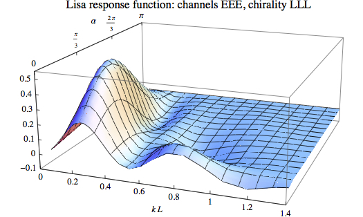
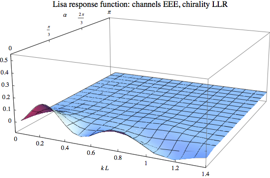
Figure 7: Amplitude of the LISA three-point response function ${\cal R}$ for signals travelling on the interferometer E channel. We provide the response functions for two choices of helicity combinations of the primordial tensor bispectrum, Left-Left-Left and Left-Left-Right. See the text for details.

Even a quick visual analysis of these plots allows us to derive some general physical consequences: we learn that in both cases, LLL and LLR, the amplitude of the three-point response function smoothly depends on the shape of the triangle, while strongly depends on the momentum scale one considers, with an oscillatory behaviour as a function of momenta. For the case of LLL helicities, at a fixed momentum scale of order $kL\simeq 0.2$, the response function is maximal around configurations near equilateral shapes (actually for $\alpha\simeq\pi/2$), and smoothly decreases towards squeezed or folded configurations. The behavior is opposite for LLR helicities, where squeezed configurations are enhanced, while the amplitude of the response function rapidly decreases towards equilateral and folded shapes. These considerations are interesting when applied to models of inflation with enhanced tensor fluctuations, and that priviledge some helicity components of the bispectrum with respect to others – for example due to parity violating interactions of the inflaton with gauge fields. When accompanied by the interactions we consider with extra spin-2 fields, these scenarios can lead to a rich phenomenology for shape and chirality dependence of the tensor bispectrum. These can in principle be tested at interferometers exploiting the shape of momentum dependences of the instrument response function. A more detailed analysis of the capabilities of LISA to detect tensor non-Gaussianities of intermediate shapes – including the computation of the corresponding signal-to-point ratio as done in [42] for equilateral configurations – is left for future work.

4 Conclusions

The use of laser interferometers to detect gravitational waves has already proven spectacularly successful. Several detection events resulted in a wealth of new information: from bounds on the speed of propagation for gravitational waves (and corresponding constraints on e.g. modified gravity models) to signatures of the production of heavy elements, such as gold, as a result of neutron stars collision. Remarkably, besides celebrated CMB probes, also the newly acquired sensitivity to gravitational radiation at interferometer scales has the potential to inform us about one of the earliest epochs in the universe history: inflation. The universe make-up during this early acceleration phase may indeed be imprinted in the correlations functions of tensor fluctuations of the metric field.
The simplest inflationary scenarios posit a PGW spectrum which is a slightly decreasing function of the wavenumber $k$ and deliver small tensor higher-point statistics. Extrapolating from known upper bounds on the signal at CMB scales, one may conclude that the standard single-field paradigm would evade constraints from both LIGO and LISA. Intriguingly, a much more dramatic outcome is predicted by entire classes of inflationary models. What these have in common is the existence of a rich particle content during inflation. As we have seen, it is rather useful in this context to classify particles according to their spin: the corresponding unitarity constraints will reflect directly on their mass range and, in turn, this will affect their impact on cosmological observables, including the gravitational waves spectrum and higher-order correlations functions, i.e. tensor non-Gaussianities. Higher-spin fields are most affected, so much so that non-minimal coupling with the inflaton sector is typically necessary to enhance their impact on the tensor sector all the way to e.g. a LISA detection. A PGW detection (or lack theoreof) at intereferometer scales then inevitably tells us about the mass, the spin and also the coupling of the inflationary particle zoo.
In this work, we have adopted the EFT approach of [1] to investigate in all generality the imprints on primordial tensor non-Gaussianities of an extra spin-2 field with sizable coupling to the inflaton field. We find that, as expected, a small sound speed for the extra field, $\sigma$, delivers a large signal. The corresponding bispectrum shape-function interpolates, as one decreases the mass $m_{\sigma}$, from the equilateral to the local profile, in complete analogy with non-Gaussianities in the scalar sector of quasi-single-field [19] inflation.
Given that a blue tensor spectrum is allowed within the EFT set-up, we also provide an estimate of the response function of the LISA interferometer in momentum configurations that interpolate between the local, the equilateral, and the flattened. We do so for two combinations of the helicities, LLL and LLR, finding that the two respond differently to different momenta configurations. These are promising results that call for a more detailed characterization of the capabilities of LISA to constrain tensor non-Gaussianities of intermediate shapes.

Appendix A Bispectrum computation

The equation of motion for $\sigma_{k}$ to leading order in slow-roll reads

$$\sigma_{k}^{{}^{\prime\prime}}-\frac{2}{\tau}\sigma_{k}^{{}^{\prime}}+\left(c_{\sigma}^{2}k^{2}+\frac{m^{2}}{H^{2}\tau^{2}}\right)\sigma_{k}=0\,,$$ (A.1)

whose solution is given in Eq. (3.3).

The diagram in Fig. 1 is computed using the in-in formula (see e.g. [44, 45])

$$\left\langle\gamma^{3}\right\rangle=\left\langle 0\,\Big{|}\left[\bar{T}\,\exp\left(i\int_{t_{0}}^{t}dt^{{}^{\prime}}H_{I}(t^{{}^{\prime}})\right)\right]\gamma^{3}_{I}\left[T\,\exp\left(-i\int_{t_{0}}^{t}dt^{{}^{\prime\prime}}H_{I}(t^{{}^{\prime\prime}})\right)\right]\Big{|}\,0\right\rangle\,,$$ (A.2)

where the subscript $I$ stands for fields in the interaction picture, $\bar{T}$ and $T$ are, respectively, anti-time ordering and time-ordering operators and the interaction Hamiltonian is given by

$$\mathcal{H}=\mathcal{H}_{2}+\mathcal{H}_{3}\,,\quad\quad\mathcal{H}_{2}=-\frac{\rho\,M_{\text{Pl}}}{2}\,a^{3}\sigma^{ij}\dot{\gamma}_{ij}\,,\quad\quad\mathcal{H}_{3}=\mu\,a^{3}\,\sigma_{ij}^{3}\,.$$ (A.3)

The Fourier expansion of the spin-2 field fluctuations was given in Eq. (3.1), where

$$\gamma^{\lambda}_{\textbf{k}}(\tau)=a_{\textbf{k}}^{\lambda}\gamma_{k}^{\lambda}(\tau)+a_{-\textbf{k}}^{\lambda\dagger}\gamma_{k}^{\lambda*}(\tau)\,,$$ (A.4)

$$\sigma^{\lambda}_{\textbf{k}}(\tau)=b_{\textbf{k}}^{\lambda}\sigma_{k}^{\lambda}(\tau)+b_{-\textbf{k}}^{\lambda\dagger}\sigma_{k}^{\lambda*}(\tau)\,,$$ (A.5)

with creation and annihilation operators obeying the commutation relations

$$\left[a^{\lambda_{1}}_{\textbf{k}_{1}},a^{\lambda_{2}\,\dagger}_{-\textbf{k}_{2}}\right]=(2\pi)^{3}\delta_{\lambda_{1}\lambda_{2}}\delta^{(3)}(\textbf{k}_{1}+\textbf{k}_{2})\,\quad\quad\left[b^{\lambda_{1}}_{\textbf{k}_{1}},b^{\lambda_{2}\,\dagger}_{-\textbf{k}_{2}}\right]=(2\pi)^{3}\delta_{\lambda_{1}\lambda_{2}}\delta^{(3)}(\textbf{k}_{1}+\textbf{k}_{2})\,.$$ (A.6)

In order to quickly illustrate the calculations, we report below the schematic form of the bispectrum

$$\langle\gamma_{\textbf{k}_{1}}^{\lambda_{1}}\gamma_{\textbf{k}_{2}}^{\lambda_{2}}\gamma_{\textbf{k}_{3}}^{\lambda_{3}}\rangle\sim\gamma_{\textbf{k}_{1}}^{\lambda_{1}}\gamma_{\textbf{k}_{2}}^{\lambda_{2}}\gamma_{\textbf{k}_{3}}^{\lambda_{3}}\,\,\Pi_{n=1,2,3}\int d^{4}x_{n}\,a^{3}(\tau_{n})\dot{\gamma}_{ij}(x_{n})\,\sigma^{ij}(x_{n})\int d^{4}y\,\,a^{3}(\tau_{y})\sigma_{ij}^{3}(y)\,.\\$$

Each contraction of the $\gamma$ fields with one another yields delta functions in momentum and helicity (and likewise for the $\sigma$ fields), reducing the initial nine polarization tensors down to three, hence the coefficient $\epsilon^{\lambda_{1}}_{\alpha\beta}(-\hat{k}_{1})\epsilon^{\lambda_{2}}_{\beta\gamma}(-\hat{k}_{2})\epsilon^{\lambda_{3}}_{\gamma\alpha}(-\hat{k}_{3})$ in Eq. (3.6). In deriving the latter we made use of the following relations:

$$\epsilon^{L/R}_{ij}(\hat{k})\cdot\epsilon^{R/L}_{ij}(\hat{k})=1\,,\quad\quad\epsilon^{L/R}_{ij}(\hat{k})\cdot\epsilon^{L/R}_{ij}(\hat{k})=0\,,$$ (A.7)

where $\epsilon^{R/L*}_{ij}(\hat{k})=\epsilon^{R/L}_{ij}(-\hat{k})=\epsilon^{L/R}_{ij}(\hat{k})$. One can rewrite the overall coefficient as follows

$$\epsilon^{\lambda_{1}}_{\alpha\beta}(\hat{k}_{1})\epsilon^{\lambda_{2}}_{\beta\gamma}(\hat{k}_{2})\epsilon^{\lambda_{3}}_{\gamma\alpha}(\hat{k}_{3}) = -\frac{1}{64\,r_{2}^{2}r_{3}^{2}}\left[2r_{2}+\left(1+r_{2}^{2}-r_{3}^{2}\right)\lambda_{1}\lambda_{2}\right]\left[-2r_{3}+\left(-1+r_{2}^{2}-r_{3}^{2}\right)\lambda_{1}\lambda_{3}\right]$$ (A.8)

$$\quad\quad\times\left[2r_{2}r_{3}+\left(-1+r_{2}^{2}+r_{3}^{2}\right)\lambda_{2}\lambda_{3}\right]$$

where $r_{2}\equiv k_{2}/k_{1}$ and $r_{3}\equiv k_{3}/k_{1}$. Eq. (A.8) has been obtained by choosing a reference triangle for the wave vectors that sits on the $(x,y)$ plane:

$$\epsilon^{R/L}_{ij}\left(\theta=\frac{\pi}{2},\varphi\right)=\frac{1}{2}\left[{\begin{array}[]{ccc}-\sin^{2}\varphi&\cos\varphi\sin\varphi&\pm i\sin\varphi\\ \cos\varphi\sin\varphi&-\cos^{2}\varphi&\mp i\cos\varphi\\ \pm i\sin\varphi&\mp i\cos\varphi&1\\ \end{array}}\right]\,.$$ (A.9)

One can set $\varphi_{1}$ to zero, hence $\varphi_{2}$ and $\varphi_{3}$ are the angles between, respectively, $\textbf{k}_{2}$ and $\textbf{k}_{1}$ and $\textbf{k}_{3}$ and $\textbf{k}_{1}$.

The expression for the bispectrum is given by the sum of three contributions (see also [19])

$$B_{(\sigma)}(k_{1},k_{2},k_{3})=B^{(A)}(k_{1},k_{2},k_{3})+B^{(B)}(k_{1},k_{2},k_{3})+B^{(C)}(k_{1},k_{2},k_{3})$$ (A.10)

where

$$B^{(A)} = 12\cdot\pi^{3}\left(\frac{\mu}{H}\right)\left(\frac{\rho}{M_{\text{Pl}}}\right)^{3}\frac{1}{k_{1}k_{2}k_{3}}\int_{-\infty}^{0}d\tau_{1}\int_{-\infty}^{\tau_{1}}d\tau_{2}\int_{-\infty}^{\tau_{2}}d\tau_{3}\int_{-\infty}^{\tau_{3}}d\tau_{4}\sqrt{\frac{\tau_{2}}{\tau_{1}\tau_{3}\tau_{4}}}$$

$$\times\text{Im}\left[e^{ik_{2}\tau_{3}}\mathcal{H}^{(1)}_{\nu}[-c_{\sigma}k_{2}\tau_{2}]\mathcal{H}^{(2)}_{\nu}[-c_{\sigma}k_{2}\tau_{3}]\right]\text{Im}\left[\mathcal{H}^{(1)}_{\nu}[-c_{\sigma}k_{1}\tau_{1}]\mathcal{H}^{(2)}_{\nu}[-c_{\sigma}k_{1}\tau_{2}]\right]$$

$$\times\left[e^{-ik_{3}\tau_{4}}\mathcal{H}^{(1)}_{\nu}[-c_{\sigma}k_{3}\tau_{4}]\mathcal{H}^{(2)}_{\nu}[-c_{\sigma}k_{3}\tau_{2}]\right]\sin[-k_{1}\tau_{1}]+\text{5\,perms}\,,$$

$$B^{(B)} = 12\cdot\pi^{3}\left(\frac{\mu}{H}\right)\left(\frac{\rho}{M_{\text{Pl}}}\right)^{3}\frac{1}{k_{1}k_{2}k_{3}}\int_{-\infty}^{0}d\tau_{1}\int_{-\infty}^{\tau_{1}}d\tau_{2}\int_{-\infty}^{\tau_{2}}d\tau_{3}\int_{-\infty}^{\tau_{3}}d\tau_{4}\sqrt{\frac{\tau_{3}}{\tau_{1}\tau_{2}\tau_{4}}}$$

$$\times\text{Im}\left[\mathcal{H}^{(1)}_{\nu}[-c_{\sigma}k_{1}\tau_{3}]\mathcal{H}^{(1)}_{\nu}[-c_{\sigma}k_{2}\tau_{3}]\mathcal{H}^{(2)}_{\nu}[-c_{\sigma}k_{1}\tau_{1}]\mathcal{H}^{(2)}_{\nu}[-c_{\sigma}k_{2}\tau_{2}]\right]$$

$$\times\text{Im}\left[e^{ik_{3}\tau_{4}}\mathcal{H}^{(1)}_{\nu}[-c_{\sigma}k_{3}\tau_{3}]\mathcal{H}^{(2)}_{\nu}[-c_{\sigma}k_{3}\tau_{4}]\right]\sin[-k_{1}\tau_{1}]\sin[-k_{2}\tau_{2}]+\text{5\,perms}\,,$$

$$B^{(C)} = 12\cdot\pi^{3}\left(\frac{\mu}{H}\right)\left(\frac{\rho}{M_{\text{Pl}}}\right)^{3}\frac{1}{k_{1}k_{2}k_{3}}\int_{-\infty}^{0}d\tau_{1}\int_{-\infty}^{\tau_{1}}d\tau_{2}\int_{-\infty}^{\tau_{2}}d\tau_{3}\int_{-\infty}^{\tau_{3}}d\tau_{4}\sqrt{\frac{\tau_{4}}{\tau_{1}\tau_{2}\tau_{3}}}$$

$$\times\text{Im}\Big{[}\mathcal{H}^{(1)}_{\nu}[-c_{\sigma}k_{1}\tau_{4}]\mathcal{H}^{(1)}_{\nu}[-c_{\sigma}k_{2}\tau_{4}]\mathcal{H}^{(1)}_{\nu}[-c_{\sigma}k_{3}\tau_{4}]\mathcal{H}^{(2)}_{\nu}[-c_{\sigma}k_{1}\tau_{1}]$$

$$\times\mathcal{H}^{(2)}_{\nu}[-c_{\sigma}k_{2}\tau_{2}]\mathcal{H}^{(2)}_{\nu}[-c_{\sigma}k_{3}\tau_{3}]\Big{]}\sin[-k_{1}\tau_{1}]\sin[-k_{2}\tau_{2}]\sin[-k_{3}\tau_{3}]+\text{5\,perms}\,.$$

From here on it is convenient to introduce the variables: $x_{i}\equiv k_{1}\tau_{i}$. The complete expression of the bispectrum then becomes (3.8), with $\mathcal{F}_{\nu c_{\sigma}}=\mathcal{F}^{A}_{\nu c_{\sigma}}+\mathcal{F}^{B}_{\nu c_{\sigma}}+\mathcal{F}^{C}_{\nu c_{\sigma}}$, where

$$\mathcal{F}^{A}_{\nu c_{\sigma}} \equiv \int\Pi_{i}dx_{i}\,\sqrt{\frac{x_{2}}{x_{1}x_{3}x_{4}}}\sin[-x_{1}]\text{Im}\left[e^{-i(k_{3}/k_{1})x_{4}}\mathcal{H}^{(1)}_{\nu}[-c_{\sigma}(k_{3}/k_{1})x_{4}]\mathcal{H}^{(2)}_{\nu}[-c_{\sigma}(k_{3}/k_{1})x_{2}]\right]$$

$$\text{Im}\left[e^{i(k_{2}/k_{1})x_{3}}\mathcal{H}^{(1)}_{\nu}[-c_{\sigma}(k_{2}/k_{1})x_{2}]\mathcal{H}^{(2)}_{\nu}[-c_{\sigma}(k_{2}/k_{1})x_{3}]\right]\text{Im}\left[\mathcal{H}^{(1)}_{\nu}[-c_{\sigma}x_{1}]\mathcal{H}^{(2)}_{\nu}[-c_{\sigma}x_{2}]\right]\,,$$

(A.14)

$$\mathcal{F}^{B}_{\nu c_{\sigma}} \equiv -\int\Pi_{i}dx_{i}\,\sqrt{\frac{x_{3}}{x_{1}x_{2}x_{4}}}\text{Im}\left[\mathcal{H}^{(1)}_{\nu}[-c_{\sigma}x_{3}]\mathcal{H}^{(1)}_{\nu}[-c_{\sigma}(k_{2}/k_{1})x_{3}]\mathcal{H}^{(2)}_{\nu}[-c_{\sigma}x_{1}]\mathcal{H}^{(2)}_{\nu}[-c_{\sigma}(k_{2}/k_{1})x_{2}]\right]$$ (A.15)

$$\text{Im}\left[e^{i(k_{3}/k_{1})x_{4}}\mathcal{H}^{(1)}_{\nu}[-c_{\sigma}(k_{3}/k_{1})x_{3}]\mathcal{H}^{(2)}_{\nu}[-c_{\sigma}(k_{3}/k_{1})x_{4}]\right]\sin[-x_{1}]\sin[-(k_{2}/k_{1})x_{2}],{\color[rgb]{1,1,1}niiiiin}$$

$$\mathcal{F}^{C}_{\nu c_{\sigma}} \equiv \int\Pi_{i}dx_{i}\,\sqrt{\frac{x_{4}}{x_{1}x_{2}x_{3}}}\sin[-x_{1}]\sin[-(k_{2}/k_{1})x_{2}]\sin[-(k_{3}/k_{1})x_{2}]$$

$$\text{Im}\Big{[}\mathcal{H}^{(1)}_{\nu}[-c_{\sigma}x_{4}]\mathcal{H}^{(1)}_{\nu}[-c_{\sigma}(k_{2}/k_{1})x_{4}]\mathcal{H}^{(1)}_{\nu}[-c_{\sigma}(k_{3}/k_{1})x_{4}]\mathcal{H}^{(2)}_{\nu}[-c_{\sigma}x_{1}]$$

$$\quad\quad\times\mathcal{H}^{(2)}_{\nu}[-c_{\sigma}(k_{2}/k_{1})x_{2}]\mathcal{H}^{(2)}_{\nu}[-c_{\sigma}(k_{3}/k_{1})x_{3}]\Big{]}\,,$$

where $\int\Pi_{i}dx_{i}\equiv\int_{-\infty}^{0}dx_{1}\int_{-\infty}^{x_{1}}dx_{2}\int_{-\infty}^{x_{2}}dx_{3}\int_{-\infty}^{x_{3}}dx_{4}$. In the squeezed and equilateral configurations, our results simplify and the momentum dependence can be factored out to arrive respectively at Eqs. (3.11) and Eqs.(3.12). Eq. (3.12) is an exact result. The squeezed limit expression, (3.11), is instead obtained by approximating some of the Hankel functions for small arguments. Consider for instance the contribution in Eq. (A) in the limit $k_{1}\sim k_{2}\gg k_{3}$. The second Hankel in the first line of (A) can be approximated for small values of its argument ($c_{\sigma}(k_{3}/k_{1})|x_{2}|\ll 1$):

$$\mathcal{H}^{(2)}_{\nu}[-c_{\sigma}(k_{3}/k_{1})x_{2}]\simeq i\,\frac{2^{\nu}\,\Gamma[\nu]}{\pi\,c_{\sigma}^{\nu}}\left(\frac{k_{1}}{k_{3}}\right)^{\nu}(-x_{2})^{-\nu}\,.$$ (A.17)

This expansion is justified by the fact that values $c_{\sigma}(k_{3}/k_{1})|x_{2}|\gtrsim 1$, i.e. $c_{\sigma}|x_{2}|\gg 1$, would cause some of the Hankel in the second line, specifically those of argument $c_{\sigma}(k_{2}/k_{1})x_{2}\simeq c_{\sigma}x_{2}$, to undergo fast oscillations, suppressing the value of the integral. Following similar reasonings, it is also possible to isolate one of the chain integrals (as the result in (3.11) shows, where we set $y_{4}\equiv(k_{3}/k_{1})x_{4}$). We verified that the leading contribution in the squeezed limit arises from the permutations spelled out in (A) and (A.15), whereas the (two, independent) remaining permutations, as well as the C-type terms as in (A), are subleading.

References

- [1] L. Bordin, P. Creminelli, A. Khmelnitsky and L. Senatore, [arXiv:1806.10587].
- [2] A. H. Guth, Phys. Rev. D 23, 347 (1981) [Adv. Ser. Astrophys. Cosmol. 3, 139 (1987)] [PhysRevD.23.347]; D. H. Lyth and A. Riotto, Phys. Rept. 314, 1 (1999) [hep-ph/9807278]; D. Baumann, [arXiv:0907.5424].
- [3] M. Kamionkowski and E. D. Kovetz, Ann. Rev. Astron. Astrophys. 54 (2016) 227 [arXiv:1510.06042]; M. C. Guzzetti, N. Bartolo, M. Liguori and S. Matarrese, Riv. Nuovo Cim. 39, no. 9, 399 (2016) [arXiv:1605.01615]; C. Caprini and D. G. Figueroa, [arXiv:1801.04268].
- [4] M. M. Anber and L. Sorbo, Phys. Rev. D 81, 043534 (2010) [arXiv:0908.4089]; L. Sorbo, JCAP 1106, 003 (2011) [arXiv:1101.1525]; A. Maleknejad and M. M. Sheikh-Jabbari, Phys. Lett. B 723, 224 (2013) [arXiv:1102.1513]; J. L. Cook and L. Sorbo, Phys. Rev. D 85, 023534 (2012) Erratum: [Phys. Rev. D 86, 069901 (2012)] [arXiv:1109.0022]; P. Adshead and M. Wyman, Phys. Rev. Lett. 108, 261302 (2012) [arXiv:1202.2366]; E. Martinec, P. Adshead and M. Wyman, JHEP 1302, 027 (2013) [arXiv:1206.2889]; N. Barnaby, J. Moxon, R. Namba, M. Peloso, G. Shiu and P. Zhou, Phys. Rev. D 86, 103508 (2012) [arXiv:1206.6117]; E. Dimastrogiovanni, M. Fasiello and A. J. Tolley, JCAP 1302, 046 (2013) [arXiv:1211.1396]; A. Maleknejad, M. M. Sheikh-Jabbari and J. Soda, Phys. Rept. 528, 161 (2013) [arXiv:1212.2921]; E. Dimastrogiovanni and M. Peloso, Phys. Rev. D 87, no. 10, 103501 (2013) [arXiv:1212.5184]; S. Mukohyama, R. Namba, M. Peloso and G. Shiu, JCAP 1408, 036 (2014) [arXiv:1405.0346]; R. Namba, M. Peloso, M. Shiraishi, L. Sorbo and C. Unal, JCAP 1601, no. 01, 041 (2016) [arXiv:1509.07521]; I. Obata and J. Soda, Phys. Rev. D 93, no. 12, 123502 (2016) Addendum: [Phys. Rev. D 95, no. 10, 109903 (2017)] [arXiv:1602.06024]; P. Adshead, E. Martinec, E. I. Sfakianakis and M. Wyman, JHEP 1612, 137 (2016) [arXiv:1609.04025]; J. Garcia-Bellido, M. Peloso and C. Unal, JCAP 1612, no. 12, 031 (2016) [arXiv:1610.03763]; P. Adshead and E. I. Sfakianakis, JHEP 1708, 130 (2017) [arXiv:1705.03024]; R. R. Caldwell and C. Devulder, Phys. Rev. D 97, no. 2, 023532 (2018) [arXiv:1706.03765]; B. Thorne, T. Fujita, M. Hazumi, N. Katayama, E. Komatsu and M. Shiraishi, Phys. Rev. D 97, no. 4, 043506 (2018) [arXiv:1707.03240]; E. Dimastrogiovanni, M. Fasiello, R. J. Hardwick, H. Assadullahi, K. Koyama and D. Wands, [arXiv:1806.05474]; E. McDonough and S. Alexander, [arXiv:1806.05684]; V. Domcke, B. Mares, F. Muia and M. Pieroni, [arXiv:1807.03358]; A. Maleknejad and E. Komatsu, [arXiv:1808.09076].
- [5] M. Biagetti, M. Fasiello and A. Riotto, Phys. Rev. D 88, 103518 (2013) [arXiv:1305.7241]; M. Biagetti, E. Dimastrogiovanni, M. Fasiello and M. Peloso, JCAP 1504, 011 (2015) [arXiv:1411.3029]; T. Fujita, J. Yokoyama and S. Yokoyama, PTEP 2015, 043E01 (2015) [arXiv:1411.3658].
- [6] N. Bartolo et al., JCAP 1612 (2016) no.12, 026 [arXiv:1610.06481].
- [7] Y. Akrami et al. [Planck Collaboration], [arXiv:1807.06211].
- [8] B. P. Abbott et al. , Phys. Rev. Lett. 118, no. 12, 121101 (2017) Erratum: [Phys. Rev. Lett. 119, no. 2, 029901 (2017)] [arXiv:1612.02029].
- [9] R. D. Peccei and H. R. Quinn, Phys. Rev. D 16, 1791 (1977). R. D. Peccei and H. R. Quinn, Phys. Rev. Lett. 38, 1440 (1977).
- [10] E. Pajer and M. Peloso, Class. Quant. Grav. 30, 214002 (2013) [arXiv:1305.3557].
- [11] K. Freese, J. A. Frieman and A. V. Olinto, Phys. Rev. Lett. 65, 3233 (1990).
- [12] N. Barnaby, J. Moxon, R. Namba, M. Peloso, G. Shiu and P. Zhou, Phys. Rev. D 86, 103508 (2012) [arXiv:1206.6117]; S. Mukohyama, R. Namba, M. Peloso and G. Shiu, JCAP 1408, 036 (2014) [arXiv:1405.0346]; E. Dimastrogiovanni, M. Fasiello and T. Fujita, JCAP 1701, no. 01, 019 (2017) [arXiv:1608.04216].
- [13] M. Mylova, O. Ozsoy, S. Parameswaran, G. Tasinato and I. Zavala, [arXiv:1808.10475].
- [14] M. C. Guzzetti, N. Bartolo, M. Liguori and S. Matarrese, Riv. Nuovo Cim. 39, no. 9, 399 (2016) [arXiv:1605.01615].
- [15] C. Cheung, P. Creminelli, A. L. Fitzpatrick, J. Kaplan and L. Senatore, JHEP 0803, 014 (2008) [arXiv:0709.0293].
- [16] A. Higuchi, Nucl. Phys. B 282, 397 (1987). M. Fasiello and A. J. Tolley, JCAP 1211, 035 (2012) [arXiv:1206.3852]. A. Kehagias and A. Riotto, JCAP 1707, no. 07, 046 (2017) [arXiv:1705.05834].
- [17] M. Fasiello and A. J. Tolley, JCAP 1312, 002 (2013) [arXiv:1308.1647].
- [18] H. Lee, D. Baumann and G. L. Pimentel, JHEP 1612, 040 (2016) [arXiv:1607.03735].
- [19] X. Chen and Y. Wang, JCAP 1004, 027 (2010) [arXiv:0911.3380]. X. Chen and Y. Wang, Phys. Rev. D 81, 063511 (2010) [arXiv:0909.0496]; E. Sefusatti, J. R. Fergusson, X. Chen and E. P. S. Shellard, JCAP 1208, 033 (2012) [arXiv:1204.6318].
- [20] M. Biagetti, E. Dimastrogiovanni and M. Fasiello, JCAP 1710, no. 10, 038 (2017) [arXiv:1708.01587]; E. Dimastrogiovanni, M. Fasiello and G. Tasinato, JCAP 1808, no. 08, 016 (2018) [arXiv:1806.00850].
- [21] N. Arkani-Hamed, H. Georgi and M. D. Schwartz, Annals Phys. 305, 96 (2003) [hep-th/0210184].
- [22] L. Senatore and M. Zaldarriaga, JHEP 1204, 024 (2012) [arXiv:1009.2093].
- [23] D. Wands, Lect. Notes Phys. 738, 275 (2008) [astro-ph/0702187].
- [24] N. Arkani-Hamed and J. Maldacena, [arXiv:1503.08043].
- [25] A. Moradinezhad Dizgah, G. Franciolini, A. Kehagias and A. Riotto, Phys. Rev. D 98, no. 6, 063520 (2018) [arXiv:1805.10247]; G. Franciolini, A. Kehagias, A. Riotto and M. Shiraishi, Phys. Rev. D 98, no. 4, 043533 (2018) [arXiv:1803.03814]; N. Bartolo, A. Kehagias, M. Liguori, A. Riotto, M. Shiraishi and V. Tansella, Phys. Rev. D 97, no. 2, 023503 (2018) [arXiv:1709.05695].
- [26] S. Deser and R. I. Nepomechie, Annals Phys. 154, 396 (1984).
- [27] S. Deser and A. Waldron, Nucl. Phys. B 607, 577 (2001) [hep-th/0103198].
- [28] C. de Rham, K. Hinterbichler, R. A. Rosen and A. J. Tolley, Phys. Rev. D 88, no. 2, 024003 (2013) [arXiv:1302.0025].
- [29] C. de Rham, Living Rev. Rel. 17, 7 (2014) [arXiv:1401.4173].
- [30] E. P. Wigner, Annals Math. 40, 149 (1939) [www.jstor.org].
- [31] T. Matsumura et al., J. Low. Temp. Phys. 176, 733 (2014) [arXiv:1311.2847].
- [32] K. N. Abazajian et al. [CMB-S4 Collaboration], “CMB-S4 Science Book, First Edition,” [arXiv:1610.02743].
- [33] S. Endlich, A. Nicolis and J. Wang, JCAP 1310, 011 (2013) [arXiv:1210.0569]; D. Cannone, G. Tasinato and D. Wands, JCAP 1501, no. 01, 029 (2015) [arXiv:1409.6568]; D. Cannone, J. O. Gong and G. Tasinato, JCAP 1508, no. 08, 003 (2015) [arXiv:1505.05773]; A. Ricciardone and G. Tasinato, Phys. Rev. D 96, no. 2, 023508 (2017) [arXiv:1611.04516]; A. Ricciardone and G. Tasinato, JCAP 1802 (2018) no.02, 011 [arXiv:1711.02635].
- [34] P. A. R. Ade et al. [Planck Collaboration], Astron. Astrophys. 594, A17 (2016) [arXiv:1502.01592].
- [35] V. Assassi, D. Baumann and D. Green, JCAP 1211, 047 (2012) [arXiv:1204.4207].
- [36] J. R. Fergusson and E. P. S. Shellard, Phys. Rev. D 76, 083523 (2007) [astro-ph/0612713].
- [37] J. M. Maldacena, JHEP 0305, 013 (2003) [astro-ph/0210603].
- [38] J. M. Maldacena and G. L. Pimentel, JHEP 1109, 045 (2011) [arXiv:1104.2846].
- [39] A. Agrawal, [arXiv:1804.01481].
- [40] M. Shiraishi, D. Nitta and S. Yokoyama, Prog. Theor. Phys. 126 (2011) 937 [arXiv:1108.0175]; M. Shiraishi, A. Ricciardone and S. Saga, JCAP 1311 (2013) 051 [arXiv:1308.6769]; M. Shiraishi, M. Liguori and J. R. Fergusson, JCAP 1501 (2015) no.01, 007 [arXiv:1409.0265 ].
- [41] H. Audley et al. [LISA Collaboration], [arXiv:1702.00786].
- [42] N. Bartolo et al., [arXiv:1806.02819].
- [43] M. R. Adams and N. J. Cornish, Phys. Rev. D 82 (2010) 022002 [arXiv:1002.1291].
- [44] S. Weinberg, Phys. Rev. D 72, 043514 (2005) [hep-th/0506236].
- [45] P. Adshead, R. Easther and E. A. Lim, Phys. Rev. D 80, 083521 (2009) [arXiv:0904.4207].
- [46] E. Dimastrogiovanni, M. Fasiello and T. Fujita, JCAP 1701, no. 01, 019 (2017) [arXiv:1608.04216];
- [47] A. Agrawal, T. Fujita and E. Komatsu, Phys. Rev. D 97, no. 10, 103526 (2018) [arXiv:1707.03023].
- [48] A. Agrawal, T. Fujita and E. Komatsu, JCAP 1806, no. 06, 027 (2018) [arXiv:1802.09284].
- [49] A. Naskar and S. Pal, Phys. Rev. D 98, no. 8, 083520 (2018) [arXiv:1806.08178].
- [50] A. Ashoorioon, [arXiv:1810.04001].