pair2vec: Compositional Word-Pair Embeddings
for Cross-Sentence Inference

Abstract

Reasoning about implied relationships (e.g. paraphrastic, common sense, encyclopedic) between pairs of words is crucial for many cross-sentence inference problems. This paper proposes new methods for learning and using embeddings of word pairs that implicitly represent background knowledge about such relationships. Our pairwise embeddings are computed as a compositional function on word representations, which is learned by maximizing the pointwise mutual information (PMI) with the contexts in which the two words co-occur. We add these representations to the cross-sentence attention layer of existing inference models (e.g. BiDAF for QA, ESIM for NLI), instead of extending or replacing existing word embeddings. Experiments show a gain of 2.7% on the recently released SQuAD 2.0 and 1.3% on MultiNLI. Our representations also aid in better generalization with gains of around 6-7% on adversarial SQuAD datasets, and 8.8% on the adversarial entailment test set by  Glockner et al. (2018).

1 Introduction

Reasoning about relationships between pairs of words is crucial for cross sentence inference problems such as question answering (QA) and natural language inference (NLI). In NLI, for example, given the premise “golf is prohibitively expensive”, inferring that the hypothesis “golf is a cheap pastime” is a contradiction requires one to know that expensive and cheap are antonyms. Recent work Glockner et al. (2018) has shown that current models, which rely heavily on unsupervised single-word embeddings, struggle to learn such relationships. In this paper, we show that they can be learned with word pair vectors (pair2vec), which are trained unsupervised, and which significantly improve performance when added to existing cross-sentence attention mechanisms.

X	Y	Contexts
		with X and Y baths
hot	cold	too X or too Y
		neither X nor Y
		in X, Y
Portland	Oregon	the X metropolitan area in Y
		X International Airport in Y
		food X are maize, Y, etc
crop	wheat	dry X, such as Y,
		more X circles appeared in Y fields
		X OS comes with Y play
Android	Google	the X team at Y
		X is developed by Y

Table 1: Example word pairs and their contexts.

Unlike single-word representations, which typically model the co-occurrence of a target word $x$ with its context $c$, our word-pair representations are learned by modeling the three-way co-occurrence between words $(x,y)$ and the context $c$ that ties them together, as seen in Table 1. While similar training signals have been used to learn models for ontology construction Hearst (1992); Snow et al. (2005); Turney (2005); Shwartz et al. (2016) and knowledge base completion Riedel et al. (2013), this paper shows, for the first time, that large scale learning of pairwise embeddings can be used to directly improve the performance of neural cross-sentence inference models.

More specifically, we train a feedforward network $R(x,y)$ that learns representations for the individual words $x$ and $y$, as well as how to compose them into a single vector. Training is done by maximizing a generalized notion of the pointwise mutual information (PMI) among $x$, $y$, and their context $c$ using a variant of negative sampling Mikolov et al. (2013a). Making $R(x,y)$ a compositional function on individual words alleviates the sparsity that necessarily comes with embedding pairs of words, even at a very large scale.

We show that our embeddings can be added to existing cross-sentence inference models, such as BiDAF++ Seo et al. (2017); Clark and Gardner (2018) for QA and ESIM Chen et al. (2017) for NLI. Instead of changing the word embeddings that are fed into the encoder, we add the pretrained pair representations to higher layers in the network where cross sentence attention mechanisms are used. This allows the model to use the background knowledge that the pair embeddings implicitly encode to reason about the likely relationships between the pairs of words it aligns.

Experiments show that simply adding our word-pair embeddings to existing high-performing models, which already use ELMo Peters et al. (2018), results in sizable gains. We show 2.72 F1 points over the BiDAF++ model Clark and Gardner (2018) on SQuAD 2.0 Rajpurkar et al. (2018), as well as a 1.3 point gain over ESIM Chen et al. (2017) on MultiNLI Williams et al. (2018). Additionally, our approach generalizes well to adversarial examples, with a 6-7% F1 increase on adversarial SQuAD Jia and Liang (2017) and a 8.8% gain on the Glockner et al. (2018) NLI benchmark. An analysis of pair2vec on word analogies suggests that it complements the information in single-word representations, especially for encyclopedic and lexicographic relations.

2 Unsupervised Pretraining

Extending the distributional hypothesis to word pairs, we posit that similar word pairs tend to occur in similar contexts, and that the contexts provide strong clues about the likely relationships that hold between the words (see Table 1). We assume a dataset of $(x,y,c)$ triplets, where each instance depicts a word pair $(x,y)$ and the context $c$ in which they appeared. We learn two compositional representation functions, $R(x,y)$ and $C(c)$, to encode the pair and the context, respectively, as $d$-dimensional vectors (Section 2.1). The functions are trained using a variant of negative sampling, which tries to embed word pairs $(x,y)$ close to the contexts $c$ with which they appeared (Section 2.2).

2.1 Representation

Our word-pair and context representations are both fixed-length vectors, composed from individual words. The word-pair representation function $R(x,y)$ first embeds and normalizes the individual words with a shared lookup matrix $E_{a}$:

$$\mathbf{x}=\frac{E_{a}(x)}{\|E_{a}(x)\|}\qquad\mathbf{y}=\frac{E_{a}(y)}{\|E_{a}(y)\|}$$

These vectors, along with their element-wise product, are fed into a four-layer perceptron:

$$R(x,y)=MLP^{4}(\mathbf{x},\mathbf{y},\mathbf{x}\circ\mathbf{y})$$

The context $c=c_{1}...c_{n}$ is encoded as a $d$-dimensional vector using the function $C(c)$. $C(c)$ embeds each token $c_{i}$ with a lookup matrix $E_{c}$, contextualizes it with a single-layer Bi-LSTM, and then aggregates the entire context with attentive pooling:

$$\mathbf{c}_{i} =E_{c}(c_{i})$$

$$\mathbf{h_{1}...h_{n}} =\text{BiLSTM}(\mathbf{c}_{1}...\mathbf{c}_{n})$$

$$w =\text{softmax}_{i}(\mathbf{k}\mathbf{h_{i}})$$

$$C(c) =\sum_{i}w_{i}\mathbf{W}\mathbf{h}_{i}$$

where $\mathbf{W}\in\mathbb{R}^{d\times d}$ and $\mathbf{k}\in\mathbb{R}^{d}$. All parameters, including the lookup tables $E_{a}$ and $E_{c}$, are trained.

Our representation is similar to two recently-proposed frameworks by Washio and Kato (2018a, b), but differs in that: (1) they use dependency paths as context, while we use surface form; (2) they encode the context as either a lookup table or the last state of a unidirectional LSTM. We also use a different objective, which we discuss next.

2.2 Objective

To optimize our representation functions, we consider two variants of negative sampling Mikolov et al. (2013a): bivariate and multivariate. The original bivariate objective models the two-way distribution of context and (monolithic) word pair co-occurrences, while our multivariate extension models the three-way distribution of word-word-context co-occurrences. We further augment the multivariate objective with typed sampling to upsample harder negative examples. We discuss the impact of the bivariate and multivariate objectives (and other components) in Section 4.3.

Bivariate	$J_{2NS}\left(x,y,c\right)=\log\sigma\left(R(x,y)\cdot C(c)\right)+\sum_{i=1}^{k_{c}}\log\sigma\left(-R(x,y)\cdot C(c^{N}_{i})\right)$
Multivariate	$J_{3NS}\left(x,y,c\right)=J_{2NS}\left(x,y,c\right)+\sum_{i=1}^{k_{x}}\log\sigma\left(-R(x^{N}_{i},y)\cdot C(c)\right)+\sum_{i=1}^{k_{y}}\log\sigma\left(-R(x,y^{N}_{i})\cdot C(c)\right)$

Table 2: The bivariate and multivariate negative sampling objectives. The superscript ^N marks randomly sampled components, with $k_{*}$ being the negative sample size per instance. The equations present per-instance objectives.

Bivariate Negative Sampling

Our objective aspires to make $R(x,y)$ and $C(c)$ similar (have high inner products) for $(x,y,c)$ that were observed together in the data. At the same time, we wish to keep our pair vectors dis-similar from random context vectors. In a straightforward application of the original (bivariate) negative sampling objective, we could generate a negative example from each observed $(x,y,c)$ instance by replacing the original context $c$ with a randomly-sampled context $c^{N}$ (Table 2, $J_{2NS}$).

Assuming that the negative contexts are sampled from the empirical distribution $P(\cdot,\cdot,c)$ (with $P(x,y,c)$ being the portion of $(x,y,c)$ instances in the dataset), we can follow Levy and Goldberg (2014) to show that this objective converges into the pointwise mutual information (PMI) between the word pair and the context.

$$R(x,y)\cdot C(c) =\log\frac{P(x,y,c)}{k_{c}P(x,y,\cdot)P(\cdot,\cdot,c)}$$

This objective mainly captures co-occurrences of monolithic pairs and contexts, and is limited by the fact that the training data, by construction, only contains pairs occurring within a sentence. For better generalization to cross-sentence tasks, where the pair distribution differs from that of the training data, we need a multivariate objective that captures the full three-way ($x,y,c$) interaction.

Multivariate Negative Sampling

We introduce negative sampling of target words, $x$ and $y$, in addition to negative sampling of contexts $c$ (Table 2, $J_{3NS}$). Our new objective also converges to a novel multivariate generalization of PMI, different from previous PMI extensions that were inspired by information theory Van de Cruys (2011) and heuristics Jameel et al. (2018). Following Levy and Goldberg (2014), we can show that when replacing target words in addition to contexts, our objective will converge to the optimal value in Equation 1:

$$R(x,y)\cdot C(c) =\log\frac{P(x,y,c)}{Z_{x,y,c}}$$ (1)

where $Z_{x,y,c}$, the denominator, is:

$$Z_{x,y,c} =k_{c}P(\cdot,\cdot,c)P(x,y,\cdot)$$

$$+k_{x}P(x,\cdot,\cdot)P(\cdot,y,c)$$

$$+k_{y}P(\cdot,y,\cdot)P(x,\cdot,c)$$ (2)

This optimal value deviates from previous generalizations of PMI by having a linear mixture of marginal probability products in its denominator. By introducing terms such as $P(x,\cdot,c)$ and $P(\cdot,y,c)$, the objective penalizes spurious correlations between words and contexts that disregard the other target word. For example, it would assign the pattern “X is a Y” a high score with (banana, fruit), but a lower score with (cat, fruit).

Typed Sampling

In multivariate negative sampling, we typically replace $x$ and $y$ by sampling from their unigram distributions. In addition to this, we also sample uniformly from the top 100 words according to cosine similarity using distributional word vectors. This is done to encourage the model to learn relations between specific instances as opposed to more general types. For example, using California as a negative sample for Oregon helps the model to learn that the pattern “X is located in Y” fits the pair (Portland, Oregon), but not the pair (Portland, California). Similar adversarial constraints were used in knowledge base completion Toutanova et al. (2015) and word embeddings Li et al. (2017).

3 Integrating pair2vec into Models

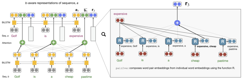
Figure 1: A typical architecture of a cross-sentence inference model (left), and how pair2vec is added to it (right). Given two sequences, $a$ and $b$, existing models create $b$-aware representations of words in $a$. For any word $a_{i}$, this typically involves the BiLSTM representation of word $a_{i}$ ($\mathbf{a}_{i}$), and an attention-weighted sum over $b$’s BiLSTM states with $a_{i}$ as the query ($\mathbf{\overline{b}}_{i}$). To these, we add the word-pair representation of $a_{i}$ and each word in $b$, weighted by attention ($\mathbf{r}_{i}$). Thicker attention arrows indicate stronger word pair alignments (e.g. cheap, expensive).

We first present a general outline for incorporating pair2vec into attention-based architectures, and then discuss changes made to BiDAF++ and ESIM. The key idea is to inject our pairwise representations into the attention layer by reusing the cross-sentence attention weights. In addition to attentive pooling over single word representations, we also pool over cross-sentence word pair embeddings (Figure 1).

3.1 General Approach

Pair Representation

We assume that we are given two sequences $a=a_{1}...a_{n}$ and $b=b_{1}...b_{m}$. We represent the word-pair embeddings between $a$ and $b$ using the pretrained pair2vec model as:

$$\mathbf{r}_{i,j}=\left[\frac{R(a_{i},b_{j})}{\|R(a_{i},b_{j})\|};\frac{R(b_{j},a_{i})}{\|R(b_{j},a_{i})\|}\right]$$ (3)

We include embeddings in both directions, $R(a_{i},b_{j})$ and $R(b_{j},a_{i})$, because the many relations can be expressed in both directions; e.g., hypernymy can be expressed via “X is a type of Y” as well as “Y such as X”. We take the $L_{2}$ normalization of each direction’s pair embedding because the heavy-tailed distribution of word pairs results in significant variance of their norms.

Base Model

Let $\mathbf{a}_{1}...\mathbf{a}_{n}$ and $\mathbf{b}_{1}...\mathbf{b}_{m}$ be the vector representations of sequences $a$ and $b$, as produced by the input encoder (e.g. ELMo embeddings contextualized with model-specific BiLSTMs). Furthermore, we assume that the base model computes soft word alignments between $a$ and $b$ via co-attention (4, 5), which are then used to compute $b$-aware representations of $a$:

$$s_{i,j} =f_{att}(\mathbf{a}_{i},\mathbf{b}_{j})$$ (4)

$$\alpha =\text{softmax}_{j}(s_{i,j})$$ (5)

$$\mathbf{\overline{b}}_{i} =\sum_{j=0}^{m}\alpha_{i,j}\mathbf{b}_{j}$$ (6)

$$\mathbf{a}_{i}^{inf} =\left[\mathbf{a}_{i};\mathbf{\overline{b}}_{i}\right]$$ (7)

The symmetric term $\mathbf{b}_{j}^{inf}$ is defined analogously. We refer to $\mathbf{a}^{inf}$ and $\mathbf{b}^{inf}$ as the inputs to the inference layer, since this layer computes some function over aligned word pairs, typically via a feedforward network and LSTMs. The inference layer is followed by aggregation and output layers.

Injecting pair2vec

We conjecture that the inference layer effectively learns word-pair relationships from training data, and it should, therefore, help to augment its input with pair2vec. We augment $\mathbf{a}_{i}^{inf}$ (7) with the pair vectors $\mathbf{r}_{i,j}$ (3) by concatenating a weighted average of the pair vectors $r_{i,j}$ involving $a_{i}$, where the weights are the same $\alpha_{i,j}$ computed via attention in (5):

$$\mathbf{r}_{i} =\sum_{j}\alpha_{i,j}\mathbf{r}_{i,j}$$ (8)

$$\mathbf{a}_{i}^{inf} =\left[\mathbf{a}_{i};\mathbf{\overline{b}}_{i};\mathbf{r}_{i}\right]$$ (9)

The symmetric term $\mathbf{b}_{j}^{inf}$ is defined analogously.

3.2 Question Answering

We augment the inference layer in the BiDAF++ model with pair2vec. BiDAF++ is an improved version of the BiDAFNoAnswer Seo et al. (2017); Levy et al. (2017) which includes self-attention and ELMo embeddings from  Peters et al. (2018). We found this variant to be stronger than the baselines presented in  Rajpurkar et al. (2018) by over 2.5 F1. We use BiDAF++ as a baseline since its architecture is typical for QA systems, and, until recently, was state-of-the-art on SQuAD 2.0 and other benchmarks.

BiDAF++

Let $\mathbf{a}$ and $\mathbf{b}$ be the outputs of the passage and question encoders respectively (in place of the standard $\mathbf{p}$ and $\mathbf{q}$ notations). The inference layer’s inputs $\mathbf{a}_{i}^{inf}$ are defined similarly to the generic model’s in (7), but also contain an aggregation of the elements in $\mathbf{a}$, with better-aligned elements receiving larger weights:

$$\mu =\text{softmax}_{i}(\max_{j}s_{i,j})$$ (10)

$$\mathbf{\hat{a}}_{i} =\sum_{i}\mu_{i}\mathbf{a}_{i}$$ (11)

$$\mathbf{a}_{i}^{inf} =\left[\mathbf{a}_{i};\mathbf{\overline{b}}_{i};\mathbf{a}_{i}\circ\mathbf{\overline{b}}_{i};\mathbf{\hat{a}}\right]$$ (12)

In the later layers, $\mathbf{a}^{inf}$ is recontextualized using a BiGRU and self attention. Finally a prediction layer predicts the start and end tokens.

BiDAF++ with pair2vec

To add our pair vectors, we simply concatenate $\mathbf{r}_{i}$ (3) to $\mathbf{a}_{i}^{inf}$ (12):

$$\mathbf{a}_{i}^{inf} =\left[\mathbf{a}_{i};\mathbf{\overline{b}}_{i};\mathbf{a}_{i}\circ\mathbf{\overline{b}}_{i};\mathbf{\hat{a}};\mathbf{r}_{i}\right]$$ (13)

3.3 Natural Language Inference

For NLI, we augment the ESIM model Chen et al. (2017), which was previously state-of-the-art on both SNLI Bowman et al. (2015) and MultiNLI Williams et al. (2018) benchmarks.

ESIM

Let $\mathbf{a}$ and $\mathbf{b}$ be the outputs of the premise and hypothesis encoders respectively (in place of the standard $\mathbf{p}$ and $\mathbf{h}$ notations). The inference layer’s inputs $\mathbf{a}_{i}^{inf}$ (and $\mathbf{b}_{j}^{inf}$) are defined similarly to the generic model’s in (7):

$$\mathbf{a}_{i}^{inf} =\left[\mathbf{a}_{i};\mathbf{\overline{b}}_{i};\mathbf{a}_{i}\circ\mathbf{\overline{b}}_{i};\mathbf{a}_{i}-\mathbf{\overline{b}}_{i}\right]$$ (14)

In the later layers, $\mathbf{a}^{inf}$ and $\mathbf{b}^{inf}$ are projected, recontextualized, and converted to a fixed-length vector for each sentence using multiple pooling schemes. These vectors are then passed on to an output layer, which predicts the class.

ESIM with pair2vec

To add our pair vectors, we simply concatenate $\mathbf{r}_{i}$ (3) to $\mathbf{a}_{i}^{inf}$ (14):

$$\mathbf{a}_{i}^{inf} =\left[\mathbf{a}_{i};\mathbf{\overline{b}}_{i};\mathbf{a}_{i}\circ\mathbf{\overline{b}}_{i};\mathbf{a}_{i}-\mathbf{\overline{b}}_{i};\mathbf{r}_{i}\right]$$ (15)

A similar augmentation of ESIM was recently proposed in KIM Chen et al. (2018). However, their pair vectors are composed of WordNet features, while our pair embeddings are learned directly from text (see further discussion in Section 6).

4 Experiments

For experiments on QA (Section 4.1) and NLI (Section 4.2), we use our full model which includes multivariate and typed negative sampling. We discuss ablations in Section 4.3

Data

We use the January 2018 dump of English Wikipedia, containing 96M sentences to train pair2vec. We restrict the vocabulary to the 100K most frequent words. Preprocessing removes all out-of-vocabulary words in the corpus. We consider each word pair within a window of 5 in the preprocessed corpus, and subsample instances based on pair probability with a threshold of $5\cdot 10^{-7}$. We define the context as one word each to the left and right, and all the words in between each pair, replacing both target words with placeholders $X$ and $Y$ (see Table 1). More details can be found in the supplementary material.

4.1 Question Answering

Benchmark		BiDAF	+ pair2vec	$\Delta$
SQuAD 2.0	EM	65.66	68.02	+2.36
	F1	68.86	71.58	+2.72
AddSent	EM	37.50	44.20	+6.70
	F1	42.55	49.69	+7.14
AddOneSent	EM	48.20	53.30	+5.10
	F1	54.02	60.13	+6.11

Table 3: Performance on SQuAD 2.0 and adversarial SQuAD (AddSent and AddOneSent) benchmarks, with and without pair2vec. All models have ELMo.

We experiment on the SQuAD 2.0 QA benchmark Rajpurkar et al. (2018), as well as the adversarial datasets of SQuAD 1.1 Rajpurkar et al. (2016); Jia and Liang (2017). Table 3 shows the performance of BiDAF++, with ELMo , before and after adding pair2vec. Experiments on SQuAD 2.0 show that our pair representations improve performance by 2.72 F1. Moreover, adding pair2vec also results in better generalization on the adversarial SQuAD datasets with gains of 7.14 and 6.11 F1.

4.2 Natural Language Inference

Benchmark	ESIM	+ pair2vec	$\Delta$
Matched	79.68	81.03	+1.35
Mismatched	78.80	80.12	+1.32

Table 4: Performance on MultiNLI, with and without pair2vec. All models have ELMo.

Model	Accuracy
Rule-based Models
WordNet Baseline	85.8
Models with GloVe
ESIM Chen et al. (2017)	77.0
KIM Chen et al. (2018)	87.7
ESIM + pair2vec	92.9
Models with ELMo
ESIM Peters et al. (2018)	84.6
ESIM + pair2vec	93.4

Table 5: Performance on the adversarial NLI test set of Glockner et al. (2018).

We report the performance of our model on MultiNLI and the adversarial test set from Glockner et al. (2018) in Table 5. We outperform the ESIM + ELMo baseline by 1.3% on the matched and mismatched portions of the dataset.

We also record a gain of 8.8% absolute over ESIM on the Glockner et al. (2018) dataset, setting a new state of the art. Following standard practice Glockner et al. (2018), we train all models on a combination of SNLI Bowman et al. (2015) and MultiNLI. Glockner et al. (2018) show that with the exception of KIM Chen et al. (2018), which uses WordNet features, several NLI models fail to generalize to this setting which involves lexical inference. For a fair comparison with KIM on the Glockner test set, we replace ELMo with GLoVE embeddings, and still outperform KIM by almost halving the error rate.

4.3 Ablations

Model	EM ($\Delta$)	F1 ($\Delta$)
pair2vec (Full Model)	69.20	72.68
Composition: 2 Layers	68.35 (-0.85)	71.65 (-1.03)
Composition: Multiply	67.10 (-2.20)	70.20 (-2.48)
Objective: Bivariate NS	68.63 (-0.57)	71.98 (-0.70)
Unsupervised: Pair Dist	67.07 (-2.13)	70.24 (-2.44)
No pair2vec (BiDAF)	66.66 (-2.54)	69.90 (-2.78)

Table 6: Ablations on the Squad 2.0 development set show that argument sampling as well as using a deeper composition function are useful.

Ablating parts of pair2vec shows that all components of the model (Section 2) are useful. We ablate each component and report the EM and F1 on the development set of SQuAD 2.0 (Table 6). The full model, which uses a 4-layer MLP for $R(x,y)$ and trains with multivariate negative sampling, achieves the highest F1 of 72.68.

We experiment with two alternative composition functions, a 2-layer MLP (Composition: 2 Layers) and element-wise multiplication (Composition: Multiply), which yield significantly smaller gains over the baseline BiDAF++ model. This demonstrates the need for a deep composition function. Eliminating sampling of target words $(x,y)$ from the objective (Objective: Bivariate NS) results in a drop of 0.7 F1, accounting for about a quarter of the overall gain. This suggests that while the bulk of the signal is mined from the pair-context interactions, there is also valuable information in other interactions as well.

We also test whether specific pre-training of word pair representations is useful by replacing pair2vec embeddings with the vector offsets of pre-trained word embeddings (Unsupervised: Pair Dist). We follow the PairDistance method for word analogies Mikolov et al. (2013b), and represent the pair $(x,y)$ as the L2 normalized difference of single-word vectors: $(\mathbf{x}-\mathbf{y})/\|\mathbf{x}-\mathbf{y}\|$. We use the same fastText  Bojanowski et al. (2017) word vectors with which we initialized pair2vec before training. We observe a gain of only 0.34 F1 over the baseline.

5 Analysis

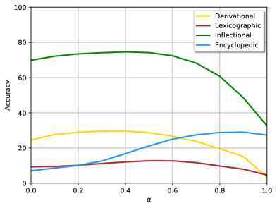
Figure 2: Accuracy as a function of the interpolation parameter $\alpha$ (see Eq. (16)). The $\alpha$=0 configuration relies only on fastText  Bojanowski et al. (2017), while $\alpha$=1 reflects pair2vec.

Relation	3CosAdd	+pair2vec	$\alpha^{*}$
Country:Capital	1.2	86.1	0.9
Name:Occupation	1.8	44.6	0.8
Name:Nationality	0.1	42.0	0.9
UK City:County	0.7	31.7	1.0
Country:Language	4.0	28.4	0.8
Verb 3pSg:Ved	49.1	61.7	0.6
Verb Ving:Ved	61.1	73.3	0.5
Verb Inf:Ved	58.5	70.1	0.5
Noun+less	4.8	16.0	0.2
Substance Meronym	3.8	14.5	0.6

Table 7: The top 10 analogy relations for which interpolating with pair2vec improves performance. $\alpha^{*}$ is the optimal interpolation parameter for each relation.

Relation	Context	X	Y (Top 3)
Antonymy/Exclusion	either X or Y	accept	reject, refuse, recognise
		hard	soft, brittle, polished
Hypernymy	including X and other Y	copper	ones, metals, mines
		google	apps, browsers, searches
Hyponymy	X like Y	cities	solaris, speyer, medina
		browsers	chrome, firefox, netscape
Co-hyponymy	, X , Y ,	copper	malachite, flint, ivory
		google	microsoft, bing, yahoo
City-State	in X , Y .	portland	oregon, maine, dorset
		dallas	tx, texas, va
City-City	from X to Y .	portland	salem, astoria, ogdensburg
		dallas	denton, allatoona, addison
Profession	X , a famous Y ,	ronaldo	footballer, portuguese, player
		monet	painter, painting, butterfly

Table 8: Given a context $c$ and a word $x$, we select the top 3 words $y$ from the entire vocabulary using our scoring function $R(x,y)\cdot C(c)$. The analysis suggests that the model tends to rank correct matches (italics) over others.

In Section 4, we showed that pair2vec adds information complementary to single-word representations like ELMo. Here, we ask what this extra information is, and try to characterize which word relations are better captured by pair2vec. To that end, we evaluate performance on a word analogy dataset with over 40 different relation types (Section 5.1), and observe how pair2vec fills hand-crafted relation patterns (Section 5.2).

5.1 Quantitative Analysis: Word Analogies

Word Analogy Dataset

Given a word pair $(a,b)$ and word $x$, the word analogy task involves predicting a word $y$ such that $a:b::x:y$. We use the Bigger Analogy Test Set (BATS, Gladkova et al., 2016) which contains four groups of relations: encyclopedic semantics (e.g., person-profession as in Einstein-physicist), lexicographic semantics (e.g., antonymy as in cheap-expensive), derivational morphology (e.g., noun forms as in oblige-obligation), and inflectional morphology (e.g., noun-plural as in bird-birds). Each group contains 10 sub-relations.

Method

We interpolate pair2vec and 3CosAdd Mikolov et al. (2013b); Levy et al. (2014) scores on fastText embeddings, as follows:

$$\textrm{score}(y) =\alpha\cdot\textrm{cos}(\mathbf{r}_{a,b},\mathbf{r}_{x,y})$$

$$+(1-\alpha)\cdot\textrm{cos}(\mathbf{b}-\mathbf{a}+\mathbf{x},\mathbf{y})$$ (16)

where $\mathbf{a}$, $\mathbf{b}$, $\mathbf{x}$, and $\mathbf{y}$ represent fastText embeddings and $\mathbf{r}_{a,b}$, $\mathbf{r}_{x,y}$ represent the pair2vec embedding for the word pairs $(a,b)$ and $(x,y)$, respectively; $\alpha$ is the linear interpolation parameter. Following prior work Mikolov et al. (2013b), we return the highest-scoring $y$ in the entire vocabulary, excluding the given words $a$, $b$, and $x$.

Results

Figure 2 shows how the accuracy on each category of relations varies with $\alpha$. For all four groups, adding pair2vec to 3CosAdd results in significant gains. In particular, the biggest relative improvements are observed for encyclopedic (356%) and lexicographic (51%) relations.

Table 7 shows the specific relations in which pair2vec made the largest absolute impact. The gains are particularly significant for relations where fastText embeddings provide limited signal. For example, the accuracy for substance meronyms goes from 3.8% to 14.5%. In some cases, there is also a synergistic effect; for instance, in noun+less, pair2vec alone scored 0% accuracy, but mixing it with 3CosAdd, which got 4.8% on its own, yielded 16% accuracy.

These results, alongside our experiments in Section 4, strongly suggest that pair2vec encodes information complementary to that in single-word embedding methods such as fastText and ELMo.

5.2 Qualitative Analysis: Slot Filling

To further explore how pair2vec encodes such complementary information, we consider a setting similar to that of knowledge base completion: given a Hearst-like context pattern $c$ and a single word $x$, predict the other word $y$ from the entire vocabulary. We rank candidate words $y$ based on the scoring function in our training objective: $R(x,y)\cdot C(c)$. We use a fixed set of example relations and manually define their predictive context patterns and a small set of candidate words $x$.

Table 8 shows the top three $y$ words. The model embeds $(x,y)$ pairs close to contexts that reflect their relationship. For example, substituting Portland in the city-state pattern (“in X, Y.”), the top two words are Oregon and Maine, both US states with cities named Portland. When used with the city-city pattern (“from X to Y.”), the top two words are Salem and Astoria, both cities in Oregon. The word-context interaction often captures multiple relations; for example, Monet is used to refer to the painter (profession) as well as his paintings.

As intended, pair2vec captures the three-way word-word-context interaction, and not just the two-way word-context interaction (as in single-word embeddings). This profound difference allows pair2vec to complement single-word embeddings with additional information.

6 Related Work

Pretrained Word Embeddings

Many state-of-the-art models initialize their word representations using pretrained embeddings such as word2vec Mikolov et al. (2013a) or ELMo Peters et al. (2018). These representations are typically trained using an interpretation of the Distributional Hypothesis Harris (1954) in which the bivariate distribution of target words and contexts is modeled. Our work deviates from the word embedding literature in two major aspects. First, our goal is to represent word pairs, not individual words. Second, our new PMI formulation models the trivariate word-word-context distribution. Experiments show that our pair embeddings can complement single-word embeddings.

Mining Textual Patterns

There is extensive literature on mining textual patterns to predict relations between words Hearst (1992); Snow et al. (2005); Turney (2005); Riedel et al. (2013); Van de Cruys (2014); Toutanova et al. (2015); Shwartz and Dagan (2016). These approaches focus mostly on relations between pairs of nouns (perhaps with the exception of VerbOcean Chklovski and Pantel (2004)). More recently, they have been expanded to predict relations between unrestricted pairs of words Jameel et al. (2018); Espinosa Anke and Schockaert (2018), assuming that each word-pair was observed together during pretraining. Washio and Kato (2018a, b) relax this assumption with a compositional model that can represent any pair, as long as each word appeared (individually) in the corpus.

These methods are evaluated on either intrinsic relation prediction tasks, such as BLESS Baroni and Lenci (2011) and CogALex Santus et al. (2016), or knowledge-base population benchmarks, e.g. FB15 Bordes et al. (2013). To the best of our knowledge, our work is the first to integrate pattern-based methods into modern high-performing semantic models and evaluate their impact on complex end-tasks like QA and NLI.

Integrating Knowledge in Complex Models

Ahn et al. (2016) integrate Freebase facts into a language model using a copying mechanism over fact attributes. Yang and Mitchell (2017) modify the LSTM cell to incorporate WordNet and NELL knowledge for event and entity extraction. For cross-sentence inference tasks, Weissenborn et al. (2017), Bauer et al. (2018), and Mihaylov and Frank (2018) dynamically refine word representations by reading assertions from ConceptNet and Wikipedia abstracts. Our approach, on the other hand, relies on a relatively simple extension of existing cross-sentence inference models. Furthermore, we do not need to dynamically retrieve and process knowledge base facts or Wikipedia texts, and just pretrain our pair vectors in advance.

KIM Chen et al. (2017) integrates word-pair vectors into the ESIM model for NLI in a very similar way to ours. However, KIM’s word-pair vectors contain only hand-engineered word-relation indicators from WordNet, whereas our word-pair vectors are automatically learned from unlabeled text. Our vectors can therefore reflect relation types that do not exist in WordNet (such as profession) as well as word pairs that do not have a direct link in WordNet (e.g. bronze and statue); see Table 8 for additional examples.

7 Conclusion and Future Work

We presented new methods for training and using word pair embeddings that implicitly represent background knowledge. Our pair embeddings are computed as a compositional function of the individual word representations, which is learned by maximizing a variant of the PMI with the contexts in which the the two words co-occur. Experiments on cross-sentence inference benchmarks demonstrated that adding these representations to existing models results in sizable improvements for both in-domain and adversarial settings.

Published concurrently with this paper, BERT  Devlin et al. (2018), which uses a masked language model objective, has reported dramatic gains on multiple semantic benchmarks including question-answering, natural language inference, and named entity recognition. Potential avenues for future work include multitasking BERT with pair2vec in order to more directly incorporate reasoning about word pair relations into the BERT objective.

Appendix A Implementation Details

Hyperparameters

For both word pairs and contexts, we use 300-dimensional word embeddings initialized with FastText Bojanowski et al. (2017). The context representation uses a single-layer Bi-LSTM with a hidden layer size of 100. We use 2 negative context samples and 3 negative argument samples for each pair-context tuple.

For pre-training, we used stochastic gradient descent with an initial learning rate of 0.01. We reduce the learning rate by a factor of 0.9 if the loss does not decrease for 300K steps. We use a batch size of 600, and train for 12 epochs.

For both end-task models, we use AllenNLP’s implementations Gardner et al. (2018) with default hyperparameters; we did not change any setting before or after injecting pair2vec. We use 0.15 dropout on our pretrained pair embeddings.

Appendix B Multivariate Negative Sampling

In this appendix, we elaborate on mathematical details of multivariate negative sampling to support our claims in Section 2.2.

B.1 Global Objective

Equation (Table 2, $J_{3NS}$) in Section 2.2 characterizes the local objective for each data instance. To understand the mathematical properties of this objective, we must first describe the global objective in terms of the entire dataset. However, this cannot be done by simply summing the local objective for each $(x,y,c)$, since each such example may appear multiple times in our dataset. Moreover, due to the nature of negative sampling, the number of times an $(x,y,c)$ triplet appears as a positive example will almost always be different from the number of times it appears as a negative one. Therefore, we must determine the frequency in which each triplet appears in each role.

We first denote the number of times the example $(x,y,c)$ appears in the dataset as $\#(x,y,c)$; this is also the number of times $(x,y,c)$ is used as a positive example. We observe that the expected number of times $(x,y,c)$ is used as a corrupt $x$ example is $k_{x}P(x,\cdot,\cdot)\#(\cdot,y,c)$, since $(x,y,c)$ can only be created as a corrupt $x$ example by randomly sampling $x$ from an example that already contained $y$ and $c$. The number of times $(x,y,c)$ is used as a corrupt $y$ or $c$ example can be derived analogously. Therefore, the global objective of our trenary negative sampling approach is:

$$J_{3NS}^{\text{Global}} =\sum_{(x,y,c)}J_{3NS}^{x,y,c}$$ (17)

$$J_{3NS}^{x,y,c} =\#(x,y,c)\cdot\log\sigma\left(S_{x,y,c}\right)$$

$$+Z_{x,y,c}^{\prime}\cdot\log\sigma\left(-S_{x,y,c}\right)$$ (18)

$$Z_{x,y,c}^{\prime} =k_{x}P(x,\cdot,\cdot)\#(\cdot,y,c)J_{-}^{x,y,c}$$

$$+k_{y}P(\cdot,y,\cdot)\#(x,\cdot,c)J_{-}^{x,y,c}$$

$$+k_{c}P(\cdot,\cdot,c)\#(x,y,\cdot)J_{-}^{x,y,c}$$ (19)

$$S_{x,y,c} =R(x,y)\cdot C(c)$$ (20)

Van de Cruys (2011)	$SI_{1}(x,y,c)$	$\log\frac{P(x,y,\cdot)P(x,\cdot,c)P(\cdot,y,c)}{P(x,\cdot,\cdot)P(\cdot,y,\cdot)P(\cdot,\cdot,c)P(x,y,c)}$
	$SI_{2}(x,y,c)$	$\log\frac{P(x,y,c)}{P(x,\cdot,\cdot)P(\cdot,y,\cdot)P(\cdot,\cdot,c)}$
Jameel et al. (2018)	$SI_{3}(x,y,c)$	$\log\frac{P(x,y,c)}{P(x,y,\cdot)P(\cdot,\cdot,c)}$
	$SI_{4}(x,y,c)$	$\log\frac{P(x,y,c)P(\cdot,\cdot,c)}{P(x,\cdot,c)P(\cdot,y,c)}$
(This Work)	$MVPMI(x,y,c)$	$\log\frac{P(x,y,c)}{k_{c}P(\cdot,\cdot,c)P(x,y,\cdot)+k_{x}P(x,\cdot,\cdot)P(\cdot,y,c)+k_{y}P(\cdot,y,\cdot)P(x,\cdot,c)}$

Table 9: Multivariate generalizations of PMI.

B.2 Relation to Multivariate PMI

With the global objective, we can now ask what is the optimal value of $S_{x,y,c}$ (20) by comparing the partial derivative of (17) to zero. This derivative is in fact equal to the partial derivative of (18), since it is the only component of the global objective in which $R(x,y)\cdot C(c)$ appears:

$$0=\frac{\partial J_{3NS}^{\text{Global}}}{\partial S_{x,y,c}}=\frac{\partial J_{3NS}^{x,y,c}}{\partial S_{x,y,c}}$$

The partial derivative of (18) can be expressed as:

$$0=\#(x,y,c)\cdot\sigma\left(-S_{x,y,c}\right)-Z_{x,y,c}^{\prime}\cdot\sigma\left(S_{x,y,c}\right)$$

which can be reformulated as:

$$S_{x,y,c}=\log\frac{\#(x,y,c)}{Z_{x,y,c}^{\prime}}$$

By expanding the fraction by $1/\#(\cdot,\cdot,\cdot)$ (i.e. dividing by the size of the dataset), we essentially convert all the frequency counts (e.g. $\#(x,y,z)$) to empirical probabilities (e.g. $P(x,y,z)$), and arrive at Equation (1) in Section 2.2.

B.3 Other Multivariate PMI Formulations

Previous work has proposed different multivariate formulations of PMI, shown in Table 9. Van de Cruys (2011) presented specific interaction information ($SI_{1}$) and specific correlation ($SI_{2}$). In addition to those metrics, Jameel et al. (2018) experimented with $SI_{3}$, which is the bivariate PMI between $(x,y)$ and $c$, and with $SI_{4}$. Our formulation deviates from previous work, and, to the best of our knowledge, cannot be trivially expressed by one of the existing metrics.

References

- Ahn et al. (2016) Sungjin Ahn, Heeyoul Choi, Tanel Pärnamaa, and Yoshua Bengio. 2016. A neural knowledge language model. arXiv preprint arXiv:1608.00318.
- Baroni and Lenci (2011) Marco Baroni and Alessandro Lenci. 2011. How we blessed distributional semantic evaluation. In Proceedings of the GEMS 2011 Workshop on GEometrical Models of Natural Language Semantics, GEMS ’11, pages 1–10, Stroudsburg, PA, USA. Association for Computational Linguistics.
- Bauer et al. (2018) Lisa Bauer, Yicheng Wang, and Mohit Bansal. 2018. Commonsense for generative multi-hop question answering tasks. In Proceedings of the 2018 Conference on Empirical Methods in Natural Language Processing, pages 4220–4230, Brussels, Belgium. Association for Computational Linguistics.
- Bojanowski et al. (2017) Piotr Bojanowski, Edouard Grave, Armand Joulin, and Tomas Mikolov. 2017. Enriching word vectors with subword information. Transactions of the Association for Computational Linguistics, 5:135–146.
- Bordes et al. (2013) Antoine Bordes, Nicolas Usunier, Alberto Garcia-Duran, Jason Weston, and Oksana Yakhnenko. 2013. Translating embeddings for modeling multi-relational data. In C. J. C. Burges, L. Bottou, M. Welling, Z. Ghahramani, and K. Q. Weinberger, editors, Advances in Neural Information Processing Systems 26, pages 2787–2795. Curran Associates, Inc.
- Bowman et al. (2015) Samuel R. Bowman, Gabor Angeli, Christopher Potts, and Christopher D. Manning. 2015. A large annotated corpus for learning natural language inference. In Proceedings of the 2015 Conference on Empirical Methods in Natural Language Processing, pages 632–642. Association for Computational Linguistics.
- Chen et al. (2018) Qian Chen, Xiaodan Zhu, Zhen-Hua Ling, Diana Inkpen, and Si Wei. 2018. Neural natural language inference models enhanced with external knowledge. In Proceedings of the 56th Annual Meeting of the Association for Computational Linguistics (Volume 1: Long Papers), pages 2406–2417. Association for Computational Linguistics.
- Chen et al. (2017) Qian Chen, Xiaodan Zhu, Zhen-Hua Ling, Si Wei, Hui Jiang, and Diana Inkpen. 2017. Enhanced LSTM for natural language inference. In Proceedings of the 55th Annual Meeting of the Association for Computational Linguistics (Volume 1: Long Papers), pages 1657–1668. Association for Computational Linguistics.
- Chklovski and Pantel (2004) Timothy Chklovski and Patrick Pantel. 2004. Verbocean: Mining the web for fine-grained semantic verb relations. In Proceedings of the 2004 Conference on Empirical Methods in Natural Language Processing.
- Clark and Gardner (2018) Christopher Clark and Matt Gardner. 2018. Simple and effective multi-paragraph reading comprehension. In Proceedings of the 56th Annual Meeting of the Association for Computational Linguistics (Volume 1: Long Papers), pages 845–855. Association for Computational Linguistics.
- Van de Cruys (2011) Tim Van de Cruys. 2011. Two multivariate generalizations of pointwise mutual information. In Proceedings of the Workshop on Distributional Semantics and Compositionality, pages 16–20. Association for Computational Linguistics.
- Van de Cruys (2014) Tim Van de Cruys. 2014. A neural network approach to selectional preference acquisition. In Proceedings of the 2014 Conference on Empirical Methods in Natural Language Processing (EMNLP), pages 26–35. Association for Computational Linguistics.
- Devlin et al. (2018) Jacob Devlin, Ming-Wei Chang, Kenton Lee, and Kristina Toutanova. 2018. BERT: Pre-training of deep bidirectional transformers for language understanding. arXiv preprint arXiv:1810.04805.
- Espinosa Anke and Schockaert (2018) Luis Espinosa Anke and Steven Schockaert. 2018. Seven: Augmenting word embeddings with unsupervised relation vectors. In Proceedings of the 27th International Conference on Computational Linguistics, pages 2653–2665. Association for Computational Linguistics.
- Gardner et al. (2018) Matt Gardner, Joel Grus, Mark Neumann, Oyvind Tafjord, Pradeep Dasigi, Nelson Liu, Matthew Peters, Michael Schmitz, and Luke Zettlemoyer. 2018. Allennlp: A deep semantic natural language processing platform. arXiv preprint arXiv:1803.07640.
- Gladkova et al. (2016) Anna Gladkova, Aleksandr Drozd, and Satoshi Matsuoka. 2016. Analogy-based detection of morphological and semantic relations with word embeddings: What works and what doesn’t. In Proceedings of the NAACL-HLT SRW, pages 47–54, San Diego, California, June 12-17, 2016. ACL.
- Glockner et al. (2018) Max Glockner, Vered Shwartz, and Yoav Goldberg. 2018. Breaking nli systems with sentences that require simple lexical inferences. In Proceedings of the 56th Annual Meeting of the Association for Computational Linguistics (Volume 2: Short Papers), pages 650–655. Association for Computational Linguistics.
- Harris (1954) Zellig Harris. 1954. Distributional structure. Word, 10(23):146–162.
- Hearst (1992) Marti Hearst. 1992. Automatic acquisition of hyponyms from large text corpora. In Proceedings of the 14th International Conference on Computational Linguistics, Nantes, France.
- Jameel et al. (2018) Shoaib Jameel, Zied Bouraoui, and Steven Schockaert. 2018. Unsupervised learning of distributional relation vectors. In Proceedings of the 56th Annual Meeting of the Association for Computational Linguistics (Volume 1: Long Papers), pages 23–33. Association for Computational Linguistics.
- Jia and Liang (2017) Robin Jia and Percy Liang. 2017. Adversarial examples for evaluating reading comprehension systems. In Proceedings of the 2017 Conference on Empirical Methods in Natural Language Processing, pages 2021–2031. Association for Computational Linguistics.
- Levy et al. (2014) Omer Levy, Ido Dagan, and Jacob Goldberger. 2014. Focused entailment graphs for open ie propositions. In Proceedings of the Eighteenth Conference on Computational Natural Language Learning, pages 87–97. Association for Computational Linguistics.
- Levy and Goldberg (2014) Omer Levy and Yoav Goldberg. 2014. Neural word embedding as implicit matrix factorization. In Proceedings of the 27th International Conference on Neural Information Processing Systems - Volume 2, NIPS’14, pages 2177–2185, Cambridge, MA, USA. MIT Press.
- Levy et al. (2017) Omer Levy, Minjoon Seo, Eunsol Choi, and Luke Zettlemoyer. 2017. Zero-shot relation extraction via reading comprehension. In Proceedings of the 21st Conference on Computational Natural Language Learning (CoNLL 2017), Vancouver, Canada, August 3-4, 2017, pages 333–342.
- Li et al. (2017) Bofang Li, Tao Liu, Zhe Zhao, Buzhou Tang, Aleksandr Drozd, Anna Rogers, and Xiaoyong Du. 2017. Investigating different syntactic context types and context representations for learning word embeddings. In Proceedings of the 2017 Conference on Empirical Methods in Natural Language Processing, pages 2421–2431. Association for Computational Linguistics.
- Mihaylov and Frank (2018) Todor Mihaylov and Anette Frank. 2018. Knowledgeable reader: Enhancing cloze-style reading comprehension with external commonsense knowledge. In Proceedings of the 56th Annual Meeting of the Association for Computational Linguistics (Volume 1: Long Papers), pages 821–832. Association for Computational Linguistics.
- Mikolov et al. (2013a) Tomas Mikolov, Ilya Sutskever, Kai Chen, Gregory S. Corrado, and Jeffrey Dean. 2013a. Distributed representations of words and phrases and their compositionality. In Advances in Neural Information Processing Systems 26: 27th Annual Conference on Neural Information Processing Systems 2013. Proceedings of a meeting held December 5-8, 2013, Lake Tahoe, Nevada, United States., pages 3111–3119.
- Mikolov et al. (2013b) Tomas Mikolov, Wen-tau Yih, and Geoffrey Zweig. 2013b. Linguistic regularities in continuous space word representations. In Proceedings of the 2013 Conference of the North American Chapter of the Association for Computational Linguistics: Human Language Technologies, pages 746–751. Association for Computational Linguistics.
- Peters et al. (2018) Matthew Peters, Mark Neumann, Mohit Iyyer, Matt Gardner, Christopher Clark, Kenton Lee, and Luke Zettlemoyer. 2018. Deep contextualized word representations. In Proceedings of the 2018 Conference of the North American Chapter of the Association for Computational Linguistics: Human Language Technologies, Volume 1 (Long Papers), pages 2227–2237. Association for Computational Linguistics.
- Rajpurkar et al. (2018) Pranav Rajpurkar, Robin Jia, and Percy Liang. 2018. Know what you don’t know: Unanswerable questions for SQuAD. In Proceedings of the 56th Annual Meeting of the Association for Computational Linguistics (Volume 2: Short Papers), pages 784–789. Association for Computational Linguistics.
- Rajpurkar et al. (2016) Pranav Rajpurkar, Jian Zhang, Konstantin Lopyrev, and Percy Liang. 2016. SQuAD: 100,000+ questions for machine comprehension of text. In Proceedings of the 2016 Conference on Empirical Methods in Natural Language Processing, pages 2383–2392, Austin, Texas. Association for Computational Linguistics.
- Riedel et al. (2013) Sebastian Riedel, Limin Yao, Benjamin M. Marlin, and Andrew McCallum. 2013. Relation extraction with matrix factorization and universal schemas. In Joint Human Language Technology Conference/Annual Meeting of the North American Chapter of the Association for Computational Linguistics (HLT-NAACL).
- Santus et al. (2016) Enrico Santus, Anna Gladkova, Stefan Evert, and Alessandro Lenci. 2016. The CogALex-V shared task on the corpus-based identification of semantic relations. In Proceedings of the 5th Workshop on Cognitive Aspects of the Lexicon (CogALex - V), pages 69–79. The COLING 2016 Organizing Committee.
- Seo et al. (2017) Minjoon Seo, Aniruddha Kembhavi, Ali Farhadi, and Hannaneh Hajishirzi. 2017. Bidirectional attention flow for machine comprehension. In Proceedings of the International Conference on Learning Representations (ICLR).
- Shwartz and Dagan (2016) Vered Shwartz and Ido Dagan. 2016. Path-based vs. distributional information in recognizing lexical semantic relations. In Proceedings of the 5th Workshop on Cognitive Aspects of the Lexicon, CogALex@COLING 2016, Osaka, Japan, December 12, 2016, pages 24–29.
- Shwartz et al. (2016) Vered Shwartz, Yoav Goldberg, and Ido Dagan. 2016. Improving hypernymy detection with an integrated path-based and distributional method. In Proceedings of the 54th Annual Meeting of the Association for Computational Linguistics (Volume 1: Long Papers), pages 2389–2398. Association for Computational Linguistics.
- Snow et al. (2005) Rion Snow, Daniel Jurafsky, and Andrew Y. Ng. 2005. Learning syntactic patterns for automatic hypernym discovery. In L. K. Saul, Y. Weiss, and L. Bottou, editors, Advances in Neural Information Processing Systems 17, pages 1297–1304. MIT Press.
- Toutanova et al. (2015) Kristina Toutanova, Danqi Chen, Patrick Pantel, Hoifung Poon, Pallavi Choudhury, and Michael Gamon. 2015. Representing text for joint embedding of text and knowledge bases. In Proceedings of the 2015 Conference on Empirical Methods in Natural Language Processing, EMNLP 2015, Lisbon, Portugal, September 17-21, 2015, pages 1499–1509.
- Turney (2005) Peter D. Turney. 2005. Measuring semantic similarity by latent relational analysis. In Proceedings of the 19th International Joint Conference on Artificial Intelligence, IJCAI’05, pages 1136–1141, San Francisco, CA, USA. Morgan Kaufmann Publishers Inc.
- Washio and Kato (2018a) Koki Washio and Tsuneaki Kato. 2018a. Filling missing paths: Modeling co-occurrences of word pairs and dependency paths for recognizing lexical semantic relations. In Proceedings of the 2018 Conference of the North American Chapter of the Association for Computational Linguistics: Human Language Technologies, Volume 1 (Long Papers), pages 1123–1133. Association for Computational Linguistics.
- Washio and Kato (2018b) Koki Washio and Tsuneaki Kato. 2018b. Neural latent relational analysis to capture lexical semantic relations in a vector space. In Proceedings of the 2018 Conference on Empirical Methods in Natural Language Processing, EMNLP 2018. Association for Computational Linguistics.
- Weissenborn et al. (2017) Dirk Weissenborn, Tomáš Kočiskỳ, and Chris Dyer. 2017. Dynamic integration of background knowledge in neural NLU systems. arXiv preprint arXiv:1706.02596.
- Williams et al. (2018) Adina Williams, Nikita Nangia, and Samuel Bowman. 2018. A broad-coverage challenge corpus for sentence understanding through inference. In Proceedings of the 2018 Conference of the North American Chapter of the Association for Computational Linguistics: Human Language Technologies, Volume 1 (Long Papers), pages 1112–1122. Association for Computational Linguistics.
- Yang and Mitchell (2017) Bishan Yang and Tom Mitchell. 2017. Leveraging knowledge bases in LSTMs for improving machine reading. In Proceedings of the 55th Annual Meeting of the Association for Computational Linguistics (Volume 1: Long Papers), pages 1436–1446. Association for Computational Linguistics.