Non-Equilibrium Field Theory for Dynamics Starting from Arbitrary Athermal Initial Conditions

Abstract

Schwinger Keldysh field theory is a widely used paradigm to study non-equilibrium dynamics of quantum many-body systems starting from a thermal state. We extend this formalism to describe non-equilibrium dynamics of quantum systems starting from arbitrary initial many-body density matrices. We show how this can be done for both Bosons and Fermions, and for both closed and open quantum systems, using additional sources coupled to bilinears of the fields at the initial time, calculating Green’s functions in a theory with these sources, and then taking appropriate set of derivatives of these Green’s functions w.r.t. initial sources to obtain physical observables. The set of derivatives depend on the initial density matrix. The physical correlators in a dynamics with arbitrary initial conditions do not satisfy Wick’s theorem, even for non-interacting systems. However our formalism constructs intermediate “n-particle Green’s functions” which obey Wick’s theorem and provide a prescription to obtain physical correlation functions from them. This allows us to obtain analytic answers for all physical many body correlation functions of a non-interacting system even when it is initialized to an arbitrary density matrix. We use these exact expressions to obtain an estimate of the violation of Wick’s theorem, and relate it to presence of connected multi-particle initial correlations in the system. We illustrate this new formalism by calculating density and current profiles in many body Fermionic and Bosonic open quantum systems initialized to non-trivial density matrices. We have also shown how this formalism can be extended to interacting many body systems.

The most general problem in non-equilibrium dynamics of quantum many body systems can be stated in the following way: given a many body Hamiltonian $H$, and an initial many body density matrix $\hat{\rho}_{0}$ at $t=0$, one needs to find the evolution of the density matrix $\hat{\rho}(t)$. This can then be used to calculate equal and unequal time correlation functions in the system. The information of the full many body density matrix can also be used to construct the reduced density matrix of a subsystem by tracing out remaining degrees of freedom. This leads to calculation of non-local information theoretic measures like entanglement entropy of the subsystem Eisert et al. (2010) with the rest of the degrees of freedom. In case of an open quantum system, the evolution of $\hat{\rho}(t)$ is governed by quantum master equations for Markovian dynamics Breuer and Petruccione (2002); Agarwal (1969) and more complicated equations with non-local memory kernels for non-Markovian dynamics Nakajima (1958); Zwanzig (1960); de Vega and Alonso (2017); Zhang et al. (2012); Chakraborty and Sensarma (2018). While a lot of progress has been made within this direct approach of solving the equation of motion of $\hat{\rho}(t)$, the method runs into the difficulty of dealing with a Hilbert space growing exponentially with size of the system. Several techniques Schollwöck (2011); Eisert (2013); Evenbly and Vidal (2015) have been proposed in recent years to reduce the size of the Hilbert space to be considered in the dynamics, with varying amount of success beyond one dimensional systems Stoudenmire and White (2012); Xiang et al. (2001); Evenbly and Vidal (2015).

Field theoretic techniques have been used extensively to obtain information about quantum many-body systems, both in their ground state as well as in thermal equilibrium at a finite temperature Altland and Simons (2010). This approach can be extended to non-equilibrium situations by considering the time evolution of the density matrix. The resulting Schwinger Keldysh (SK) field theory Keldysh (1965); *kamenev; *rammer_2007; Kamenev (2011), which involves two sets of fields for each space-time point, provides a path integral based approach to the non-equilibrium dynamics of quantum many body systems. However, the current formulation of SK field theory has a major drawback: it can only efficiently deal with initial density matrices which are thermal (this includes ground states). In this case, the real time path integral is extended into the Kadanoff-Baym contour Kadanoff (1962); *SciPost_Aron along the imaginary time axis. The SK field theory is also widely used in describing steady states of quantum systems where the memory of the initial condition is assumed to be erased Jauho et al. (1994); Chakraborty and Sensarma (2018). But several interesting questions in non-equilibrium dynamics of many body systems, where dependence on initial conditions need to be tracked explicitly, cannot even be posed within this formalism. This severely restricts the applicability of SK field theory. In this paper, we formulate a comprehensive action based field theoretic approach which can explicitly keep track of arbitrary initial conditions and their effect on the quantum dynamics of Bosons and Fermions. This extends the domain of applicability of SK field theory to a large class of problems hitherto inaccessible to the field theoretic approaches.

Before we describe the new formalism, we would like to point out some important questions/problems in non-equilibrium many body dynamics, where it is important to keep track of the initial conditions explicitly. (i) Quantum computation works on the principle that different initial conditions (inputs) will generically lead to different measurements (outputs) in the system Nielsen and Chuang (2010); *Qcomp_book. It is obvious that ignoring initial conditions in problems related to implementation of quantum gates would lead to trivial results. (ii) Discussion of approach to thermal equilibrium and development of quantum chaos Jensen (1992) in a many-body system requires studying dynamics starting from an initial state far from equilibrium. In fact in a chaotic system, one would expect the dynamics to be extremely sensitive to initial conditions. (iii) Integrable systems Rigol (2009); Langen et al. (2015) and many body localized systems Nandkishore and Huse (2015) retain memory of the initial state for long times and hence they do not thermalize. To capture this aspect, it is important to construct a description which explicitly takes the initial condition into account. We would like to note that the only experimental evidence  Schreiber et al. (2015); *Choi1547 for MBL is to measure the residual memory of initial state in the long time dynamics. (iv) There are quantum systems whose long time behaviour changes qualitatively depending on the initial condition, e.g. systems with mobility edges Basko et al. (2006); Nandkishore and Huse (2015) may or may not thermalize depending on the state in which they are prepared. Cold atom systems with strong non-linearity Labouvie et al. (2016) have also been found to reach qualitatively different steady states depending on initial preparation. (v) An interesting class of problems related to thermalization involves solving for the dynamics of open quantum systems (OQS)Breuer and Petruccione (2002), where a quantum system can exchange energy/particles with a large reservoir/bath. In the open quantum system set-up, it is interesting to study how the memory of the initial state of the system is being retained in its subsequent dynamics while the external dissipative effect from the baths tries to erase it, as it approaches a thermal equilibrium/non-equilibrium steady state. Interplay of multiple time scales, governing the inherent dynamics of the system and the relaxation coming from the external bath, make this problem particularly interesting. (vi) Recent advances in ultra-fast spectroscopy has led to the study of transient quantum transportYu et al. (2016); *transient2; *transient3; *transient4; *transient5; *transient6; *transient7; *transient8 in condensed matter systems, where the system is initialized to a highly excited state and the change in its transport properties are measured. The full counting statistics of charge and spin in these systems Esposito et al. (2009); Tang and Wang (2014); Tang et al. (2014) measure highly non-linear response in these time-evolving systems. A proper investigation of these properties also require a formalism to treat athermal initial conditions. (vii) Problems related to aging in quantum glasses also require a description of dynamics starting from non-equilibrium initial conditions. Cugliandolo et al. (2006); *aging2; *aging This is not an exhaustive list, but provides some context as to why such a formalism is important to develop.

There have been two major streams of attempts in the past to include arbitrary initial conditions within a field theoretic approach. The first one starts from the Martin-Schwinger hierarchical equation Baym and Kadanoff (1961) for the one-particle Green’s function and then tries to include initial correlations in different ways. In this case one assumes a Dyson equation with a self energy structure, and then modifies the self energy to satisfy initial boundary conditions Semkat et al. (1999); *Bonitz2. There are two main problems with this approach: (i) It assumes that a Dyson equation for one-particle Green’s function can be written in terms of an irreducible self energy, which is itself a function of one particle Green’s functions, or with additive corrections representing initial correlations. Since Wick’s theorem is not valid in a theory with arbitrary initial condition (as we will show from exact expressions in our formalism), it is not clear under what condition this can be done. (ii) Singling out the one particle correlation function does not automatically provide a way to write down equations for higher order correlation functions even in a non-interacting theory Yang et al. (2014); *Zhang2; van Leeuwen and Stefanucci (2012) which will be evident from our formalism. The second approach, due to Konstantinov and Perel KONSTANTINOV and PEREL (1961), essentially states that since the density matrix is a Hermitian operator with non-negative eigenvalues, it can always be written as an exponential of some many body Hamiltonian (which can be quite different from the Hamiltonian which generates dynamics of the system) Wagner (1991); *Stefanucci_GFF; *SciPost_Aron. One can then use the old Kadanoff-Baym contour, with the dynamics along the imaginary time contour governed by this new “Hamiltonian”. However, (i) for a given generic density matrix, finding the “imaginary time Hamiltonian” requires a diagonalization in an exponentially large Hilbert space and (ii) there is no guarantee that the resulting “Hamiltonian” will be local or will only have few-body operators. Then the field theory along the imaginary time contour becomes very hard to implement. Even for systems evolving in real time with a non-interacting Hamiltonian, the arbitrary non- thermal initial state maps the problem into a non-Gaussian field theory along the imaginary time axis of the Kadanoff-Baym contour.

In this paper we will develop a unified action based description of dynamics of many Bosons/Fermions starting from arbitrary initial conditions. For this, we need to consider a SK field theory in presence of a source, $\hat{u}$ which couples to bilinears of the initial fields. We note that in contrast to the other approaches Garny and Müller (2009); van Leeuwen and Stefanucci (2012), the additional term in the action, taking care of the initial correlations, is still quadratic and do not lead to high order vertices in this theory. This source is turned on only at the initial time, i.e. it acts like an impulse. Different n-particle Green’s functions, $\hat{G}^{(n)}(u)$ are then calculated in this theory in presence of the source $\hat{u}$. The physical correlators, corresponding to dynamics starting from a particular $\hat{\rho}_{0}$, can then be obtained by taking a set of derivatives of the Green’s functions with respect to $\hat{u}$ and then setting $\hat{u}$ to zero. The particular set of derivatives to be taken depends on $\hat{\rho}_{0}$. We note that, in this formulation the calculation of the Green’s functions are universal, i.e. they do not depend on particular $\hat{\rho}_{0}$. The information of specific $\hat{\rho}_{0}$ is required solely to determine the set of derivatives (w.r.t $\hat{u}$) to be taken to obtain the physical correlators.

In this formalism, we are able to construct a set of intermediate quantities, $\hat{G}^{(n)}(u)$, which have the structure of “n-particle Green’s functions” and are derived from the action (with the source $\hat{u}$) in the usual field theoretic way; i.e. Wick’s theorem holds for these quantities. One can, for example, construct a diagrammatic perturbation theory for $\hat{G}^{(n)}(u)$ using standard rules of SK field theory. The usual paradigms of obtaining interacting Green’s functions in terms of self-energies and higher order vertex functions are valid for these quantities. These are however not the physical n-particle correlators; we provide a prescription to compute the physical correlators for different initial density matrices from these intermediate quantities. The key theoretical advance in this formalism is to prescribe a two step process: (i) construction of intermediate quantities where we can apply the well studied structures and standard approximations of SK quantum field theory, and (ii) a prescription to obtain physical correlation functions from them. We would like to emphasize that the above statements are exact even for interacting open quantum systems and do not involve any ad-hoc approximation regarding the initial correlations.

There are some other key advantages of having an action based formalism: (i) all correlation functions can be derived from a unified description by adding linear source fields $J$ to the action and then taking appropriate derivatives w.r.t $J$. Hence they are all on the same theoretical footing, as opposed to a focus on one particle correlators (ii) The general formalism keeps track of all “n-particle initial correlations”. For non-interacting theories it leads to exact answers for physical correlation functions, even for open quantum systems. This is in itself non-trivial since there is no Wick’s theorem for physical correlators. This is an advantage from the Konstantinov Perel (KP) formalism, where it is hard to get exact answers even for non-interacting theories starting from arbitrary initial condition. (iii) For interacting theories, it leads to exact expressions on which approximations have to be made for practical calculations. In this case, this formalism provides the most transparent way to understand and make useful approximations. (iv) The action principle provides a way to integrate out degrees of freedom and construct effective theories. Effective theories of dynamics starting from arbitrary initial conditions is a completely unexplored area where there may be new surprises. This may lead to a renormalization group analysis Sieberer et al. (2014); *Sangita of non-equilibrium dynamics starting from non-trivial initial conditions.

In this paper, we will set up the general formalism, but focus mainly on non-interacting systems (including open quantum systems), where we can make exact statements. We will construct the intermediate quantities for which a diagrammatic perturbation theory can be worked out in case of an interacting system, and sketch how that can be done, but we will leave the question of the different approximations and their validity in interacting systems for a future work. We will now provide a guide map for the reader to explore this paper. In section I, we have briefly outlined the structure of the standard SK field theory formalism and set up the notation to be used in this paper. In the next section II, we have explained the main idea behind the extension of the SK formalism to include arbitrary initial condition and introduce the new ingredients of the field theory. In section III, we have explicitly worked them out for a system of Bosons starting from generic density matrix in Fock space. We first consider the pedagogical case of a single Bosonic mode starting from a density matrix diagonal in the number basis and derived the corresponding formalism. We then extend this to a multi-mode system starting with density matrix diagonal in the Fock basis. Finally, we consider the extension to arbitrary initial density matrices with off-diagonal elements in the Fock basis. In section IV, we consider a Fermionic theory. A large part of the derivations of the Fermionic theory follow along lines similar to that of Bosonic theory. In this section, we mainly focus on the modifications required to convert the Bosonic theory to the Fermionic theory. In section V, we focus on calculating multi-particle physical correlators for a system of non-interacting Bosons and Fermions starting from arbitrary initial condition. We show how the Wick’s theorem is violated by explicitly computing the corrections to the Wick reconstruction of the two particle physical correlators in terms of one particle physical correlators. In section VI we extended the formalism to the case of a many body open quantum system. We also work out some examples of the above formalism to compute the evolution of densities and currents in many body open quantum systems. Finally, in section VII we sketch the general structure of the interacting theory without going into the details of the approximation strategies.

I Brief Review of Standard Schwinger-Keldysh Field Theory

We start with a brief review of the standard SK field theory Kamenev (2011), both to set up notations and to provide context for our extension of the formalism. The time evolution of a many body density matrix is given by $\hat{\rho}(t)=U(t,0)\hat{\rho}_{0}U^{\dagger}(t,0)$, where, for Hamiltonian dynamics of a closed quantum system, the time evolution operator is $U(t,0)={\cal T}[e^{-i\int_{0}^{t}dt^{\prime}H(t^{\prime})}]$. For an open quantum system, $U$ is not an unitary operator in general. In SK field theory, each of $U$ and $U^{\dagger}$ is expanded in a path/functional integral, resulting in the Keldysh partition function for Bosons

$$Z = Tr[U(\infty,0)\hat{\rho}_{0}U^{\dagger}(\infty,0)]$$

$$= \int D[\phi_{+},\phi_{-}]e^{\mathbf{i}(S[\phi_{+}]-S[\phi_{-}])}\langle\phi_{+}(0)|\hat{\rho}_{0}|\phi_{-}(0)\rangle$$

where the complex Bosonic fields $\phi_{+}$ and $\phi_{-}$ correspond to the expansion of $U$ and $U^{\dagger}$ respectively, and $|\phi\rangle$ is a many body Bosonic coherent state. Note that the time evolution operators, which result in the $e^{\pm\mathbf{i}S}$ terms, shift the trace over final states to a trace over initial states. The detailed form of $S$ is not relevant for the present discussion. For Fermionic systems, a similar expansion with Grassmann coherent states leads to

$$Z = \int D[\psi_{+},\psi_{-}]e^{\mathbf{i}(S[\psi_{+}]-S[\psi_{-}])}{\color[rgb]{0,0,0}\langle\psi_{+}(0)|\hat{\rho}_{0}|-\psi_{-}(0)\rangle}$$ (2)

where $\psi_{\pm}$ are the Grassmann fields. Note the additional minus sign in the matrix element, which comes from writing a trace in the Fermionic Fock space as integrals over Grassmann fields Negele and Orland (2002). This will be important in the detailed discussion in Section IV. Thus the SK field theory is written in terms of doubled fields in a real time formalism, with a path/functional integral over a contour shown in Fig. 1(a). It is clear that if the matrix element of $\hat{\rho}_{0}$ can be written as an exponential of a low order polynomial of the fields, one can obtain a standard action based formalism for the dynamics. This can be achieved if $\hat{\rho}_{0}$ is a thermal density matrix corresponding to a Hamiltonian $\hat{H}_{0}$ containing only a few body operators, i.e. $\hat{\rho}_{0}=exp[-\beta\hat{H}_{0}]$ ($\hat{H}_{0}$ does not need to be generator of the real time dynamics; c.f. quantum quench problems). In this case the matrix element can be written as an Euclidean path integral, and the full $Z$ is a path integral over the Kadanoff Baym contour shown in Fig. 1(b), which extends into the imaginary axis from $t=0$ to $t=-\mathbf{i}\beta$. We note that for a large class of $\hat{\rho}_{0}$, the above prescription does not work. We have already articulated the problem with the KP formalism, which tries to cast every $\hat{\rho}_{0}$ into the above mentioned formalism, even at the cost of having a $\hat{H}_{0}$ with arbitrary $n-$ particle interactions. Clearly a new formalism is required to treat the vast set of initial conditions, which do not lend themselves to a simple $\hat{H}_{0}$.

Correlation functions are calculated in SK theory by coupling sources $J_{\pm}$ linearly to the fields and taking appropriate derivatives with respect to these sources. For one-particle Green’s functions, the doubled field approach leads to redundancies, i.e. the $4$ possible Green’s functions are not independent. To make this explicit, one works with symmetric and anti-symmetric combination of the fields. For Bosons, these are called “classical” $\phi_{cl}=(\phi_{+}+\phi_{-})/\sqrt{2}$ and “quantum” fields, $\phi_{q}=(\phi_{+}-\phi_{-})/\sqrt{2}$. In this case, the quadratic action has the form

$$S=\int dt\int dt^{\prime}[\phi^{\ast}_{cl}(t),\phi^{\ast}_{q}(t)]\left[\begin{array}[]{cc}0&G^{-1}_{A}\\ G^{-1}_{R}&-\Sigma_{K}\end{array}\right]\left[\begin{array}[]{c}\phi_{cl}(t^{\prime})\\ \phi_{q}(t^{\prime})\end{array}\right]$$ (3)

We see that $S[\phi_{q}=0]=0$, a statement which holds true even when external baths and inter-particle interactions are present in the description. Here, $G_{R(A)}$ are the retarded (advanced) Green’s function, with $G_{A}=[G_{R}]^{\dagger}$, and $\Sigma_{K}$ is anti-hermitian Kamenev (2011). This leads to the following structure in Green’s functions,

$$\hat{G}(t,t^{\prime})=\left[\begin{array}[]{cc}G_{K}(t,t^{\prime})&G_{R}(t,t^{\prime})\\ G_{A}(t,t^{\prime})&0\end{array}\right]$$

where the Keldysh component $G_{K}$ is anti-hermitian. For Fermions, we follow Larkin-Ovchinikov transformation, $\psi_{1}=(\psi_{+}+\psi_{-})/\sqrt{2}$, $\psi^{\ast}_{1}=(\psi^{\ast}_{+}-\psi^{\ast}_{-})/\sqrt{2}$, $\psi_{2}=(\psi_{+}-\psi_{-})/\sqrt{2}$, and $\psi^{\ast}_{2}=(\psi^{\ast}_{+}+\psi^{\ast}_{-})/\sqrt{2}$ and get

$$S=\int dt\int dt^{\prime}[\psi^{\ast}_{1}(t),\psi^{\ast}_{2}(t)]\left[\begin{array}[]{cc}G^{-1}_{R}&-\Sigma_{K}\\ 0&G^{-1}_{A}\end{array}\right]\left[\begin{array}[]{c}\psi_{1}(t^{\prime})\\ \psi_{2}(t^{\prime})\end{array}\right]$$ (4)

In this case, $S[\psi_{1}^{\ast}=0,\psi_{2}=0]=0$ and the Green’s functions have a structure similar to that for Bosons. Note that for non-interacting theories, $\hat{G}$ is obtained simply by inverting the matrix in the microscopic action.

One can study the effects of interparticle interactions by adding terms to the Keldysh actions (eqns 3, 4). For a pairwise interacting system, the added terms are quartic in the fields. For a generic interaction, the problem cannot be solved exactly, but a diagrammatic perturbation theory can be constructed with the matrix of propagators and vertices having $cl/q$ indices along with other quantum numbers. With these changes, standard field theoretic calculations, including non-perturbative resummation of the series can be undertaken in the usual way. The SK field theory then operationally becomes equivalent to the standard field theories with this added $2-$component structure.

It is important to note that the retarded Green’s function $G_{R}(i,t;j,t^{\prime})$ has the physical interpretation of the probability amplitude of finding a particle in state $i$ at time $t$ if it is already known to be in state $j$ at some earlier time $t^{\prime}$ without creating additional excitations in the system. For non-interacting systems, this is independent of the initial conditions. For interacting systems, this amplitude does depend on initial conditions, since probability amplitude of scattering at intermediate times depend on the distribution functions, which depends on initial conditions. On the contrary, the Keldysh Green’s function explicitly keeps track of the initial conditions (e.g. it depends explicitly on the temperature of the initial distribution for thermal cases).

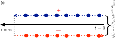
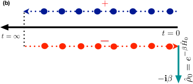
Figure 1: (a) Keldysh contours showing forward and backward propagation in time. In our formalism, the matrix element of the initial density matrix, $\hat{\rho}_{0}$ is written as the derivative of $exp[\mathbf{i}\delta S(u)]$, where $\delta S(u)$ is an added quadratic term in the action which couples to the initial bilinear source $\hat{u}$. The set of derivatives, ${\cal L}(\partial_{u},\rho_{0})$, to be taken, is completely dictated by initial $\hat{\rho}_{0}$. (b) The Kadanoff Baym contour with an extension along the imaginary time axis, from $t=0$ to $t=-\mathbf{i}\beta$, in the Konstantinov Perel formalism. In the KP formalism, $\hat{\rho}_{0}=exp(-\beta\hat{H}_{0})$, with some many body operator $\hat{H}_{0}$, is written as a path integral along the imaginary axis.

II Structure of the new formalism for Arbitrary Initial Conditions

In this section, we will describe the general structure of the formalism which allows us to treat dynamics of a system of Bosons/Fermions starting from an arbitrary initial density matrix. We will focus on the key modifications of the SK field theory required to achieve this, leaving the detailed derivation for later sections. We intend to highlight the fact that several properties, which are taken for granted in standard field theories, do not hold in this case and the ways to get around these difficulties.

We will develop our formalism for a system with large but finite number of degrees of freedom. We will consider the question of taking the continuum limit in terms of the physical correlation functions at the very end. In the new formalism, the matrix element of $\hat{\rho}_{0}$ between coherent states in Eq. I and Eq. 2 is written as a polynomial of the bi-linears of the initial fields. This can be exponentiated by adding to the standard Keldysh action, a term $\delta S$, where functions of a source field $\hat{u}$, couple to bilinears of the fields only at $t=0$. The polynomial can then be retrieved by taking appropriate derivatives of $exp[\mathbf{i}~{}\delta S(u)]$ w.r.t $\hat{u}$ and setting $\hat{u}$ to zero [Fig. 1 (a)]. The additional initial source is similar to the conjugate field in the full counting statistics *kamenev; Tang and Wang (2014), derivatives with respect to which lead to moments of the number distribution. We have replaced the arbitrary polynomial resulting from the matrix element of $\hat{\rho}_{0}$ by its generating function in our formalism. We note that our source field is quite different from the additional field of Ref. Tang and Wang, 2014, where an integral with respect to the field acts as a projector onto number states. The detailed derivation of the source function which achieves this will be slightly different for Bosons and Fermions and depends on the structure of the initial density matrix. These details will be filled in the next sections, and are cataloged in Table 1. For both Bosons and Fermions, the new term can be seen as an addition to the term $\Sigma^{K}$ in eq. 3 and eq. 4 and maintains the anti-hermiticity property of $\Sigma^{K}$. This term can be thought of as a generalized impulse potential felt by the system at the initial time.

The functional integral over the fields can be done first to obtain the partition function $Z(u)$ and the derivative w.r.t $\hat{u}$ can then be taken on this quantity to get the physical partition function corresponding to $\hat{\rho}_{0}$. On the top of this, sources $J$ which couple linearly to the fields at all times $t>0$ can be added to this action, and the functional integrals over the fields performed to yield the partition function, $Z(J,u)$. Note that $u$ and $J$ couple differently to the fields: $\hat{u}$ couples to bilinears only at $t=0$, while $J$ couples linearly at all times. This implies that no cross derivative of any quantity w.r.t $\hat{u}$ and $J$ survives when all the source fields are set to zero. Then the Green’s function in presence of $\hat{u}$ can be calculated by taking appropriate derivatives of $Z(J,u)$ with respect to $J$, and setting $J=0$. For a quadratic theory with action

$$S(u)=\int dt\int dt^{\prime}\Psi^{\dagger}(t)\hat{G}^{-1}(t,t^{\prime},u)\Psi(t^{\prime}),$$ (5)

where $\Psi^{\dagger}(t)=[\phi^{\ast}_{cl}(t),\phi^{\ast}_{q}(t)]$ for Bosons and $\Psi^{\dagger}(t)=[\psi^{\ast}_{1}(t),\psi^{\ast}_{2}(t)]$ for Fermions, the physical one particle correlation function can be obtained by taking proper derivative of ${\cal N}(u)\hat{G}(u)$, where the normalization ${\cal N}(u)=[\textrm{Det}~{}\{-\mathbf{i}\hat{G}^{-1}(u)\}]^{-\zeta}$ comes from performing the Gaussian integral, with $\zeta=\pm 1$ for Bosons (Fermions), and $\hat{G}(u)$ is the inverse of the matrix in equation 5. While $\hat{G}(u)$ is not the physical one-particle correlation function, we will see that it is an important intermediate construction, which has very useful properties and will be used many times in developing the theory. We will call this object the “Green’s function in presence of initial source $\hat{u}$”, since it is indeed the Green’s function for the saddle point equations of the action with the initial bilinear source term. We stress once again that this is not the physical one particle correlator of the system.

The physical one-particle correlator is now given by,

$$\hat{{\cal G}}_{\rho_{0}}={\cal L}(\partial_{u},\rho_{0})[{\cal N}(u)\hat{G}(u)]|_{u=0}$$ (6)

where ${\cal L}$ is a differential operator which depends on $\hat{\rho}_{0}$ and encodes initial correlations. The different forms of $\delta S$, ${\cal N}(u)$ and ${\cal L}(\partial_{u},\rho_{0})$ for a large class of initial conditions for both Bosons and Fermions are tabulated in Table 1. The detailed derivations are given in later sections of this paper. We can generalize the above procedure to the computation of a physical “n-particle correlator”, i.e

$$\hat{{\cal G}^{(n)}}_{\rho_{0}}={\cal L}(\partial_{u},\rho_{0})[{\cal N}(u)\hat{G}^{(n)}(u)]\bigg{|}_{u=0}$$ (7)

Note that the differential operator ${\cal L}$ and the normalization ${\cal N}(u)$ is the same for all order correlation functions. $\hat{G}(u)$ and $\hat{G}^{(n)}(u)$ are derived from the action $S(u)$ using standard SK field theoretic ways, i.e. initial conditions do not play a role in the derivation. Thus, $\hat{G}^{(n)}(u)$ can be easily written as a sum of products of $\hat{G}(u)$ using Wick’s theorem. This relationship is violated by the application of the differential operator ${\cal L}(\partial_{u},\rho_{0})$, i.e. ${\cal G}^{(n)}_{\rho_{0}}$ can not be written as a sum of products of ${\cal G}_{\rho_{0}}$ even for a non-interacting theory. The absence of a Wick’s theorem for physical correlators in a non-interacting theory is at the heart of all the complications in constructing physical correlators in interacting theory in terms of non-interacting correlators.

Our formalism bypasses this difficulty by constructing $\hat{G}_{int}(u)$ and $\hat{G}_{int}^{(n)}(u)$ for an interacting theory. These quantities are obtained by standard SK field theoretic techniques from an action $S(u)+S_{int}$ where $S_{int}$ represents the inter-particle interactions. The diagrammatic expansion of $\hat{G}_{int}(u)$, in terms of $\hat{G}(u)$ and the interaction vertices, follow the Feynman rules of the standard SK theory. The series can be resumed in terms of a self-energy $\Sigma[\hat{G}(u)]$ (for a perturbative expansion of $\Sigma$) or $\Sigma[\hat{G}_{int}(u)]$ (for a skeleton diagram expansion). Similarly, one can can construct $\hat{G}^{(n)}_{int}(u)$ in terms of $\hat{G}(u)$ and higher order vertex functions. All the knowledge from the standard SK field theory and different perturbative or non-perturbative approximations can be used to compute $\hat{G}_{int}(u)$ and $\hat{G}^{(n)}_{int}(u)$. We finally need to compute physical correlators, ${\cal G}^{(n)}_{\rho_{0},int}$ from $\hat{G}^{(n)}_{int}(u)$, which are once again related by eqn. 7, with $\hat{G}^{(n)}(u)$ replaced by $\hat{G}^{(n)}_{int}(u)$ and $\hat{{\cal G}}^{(n)}_{\rho_{0}}$ replaced by ${\cal G}^{(n)}_{\rho_{0},int}$.

Our formalism thus breaks up the calculation of “n-particle correlators” in an interacting theory starting from arbitrary initial conditions into $2$ parts: (i) a universal calculation of $\hat{G}_{int}(u)$ and $\hat{G}^{(n)}_{int}(u)$ which does not depend on particular choice of $\hat{\rho}_{0}$ and uses standard SK field theoretic techniques with a $\hat{u}$ dependent bare Green’s functions and (ii) obtaining ${\cal G}^{(n)}_{\rho_{0},int}$ by applying ${\cal L}(\partial_{u},\rho_{0})$ on ${\cal N}(u)\hat{G}^{(n)}_{int}(u)$. All the dependence on $\hat{\rho}_{0}$ enters in the theory through the last step. We note that there is no approximation made in the construction of the theory, i.e. all statements made above are exact. In the next sections, we provide a derivation of the theory outlined above, pointing out the details of how $\delta S$, ${\cal N}$ and ${\cal L}$ depend on the statistics of the particles and the initial density matrix $\hat{\rho}_{0}$.

System	Initial Density Matrix	$\delta S(u)$	${\cal N}(u)$	${\cal L}(\partial_{u},\rho_{0})$
	Single mode :Diagonal $\hat{\rho}_{0}$	$\mathbf{i}\phi^{\ast}_{q}(0)\phi_{q}(0)\frac{1+u}{1-u}$	$\frac{1}{1-u}$	$\sum\limits_{n}\frac{1}{n!}c_{n}\partial_{u}^{n}$
	$=\sum_{n}c_{n}|n\rangle\langle n|$
	Multi-mode :Diagonal $\hat{\rho}_{0}$	$\mathbf{i}\sum_{\alpha}\phi^{\ast}_{q}(\alpha,0)\phi_{q}(\alpha,0)\frac{1+u_{\alpha}}{1-u_{\alpha}}$	$\frac{1}{\prod_{\alpha}(1-u_{\alpha})}$	$\sum\limits_{\{n\}}c_{\{n\}}\prod_{\gamma}\frac{\partial_{u_{\gamma}}^{n_{\gamma}}}{n_{\gamma}!}$
Boson	$=\sum_{\{n\}}c_{\{n\}}|\{n\}\rangle\langle\{n\}|$
	Multi-mode :Generic $\hat{\rho}_{0}$	$\mathbf{i}\sum\limits_{\alpha\beta}\phi^{\ast}_{q}(\alpha,0)\phi_{q}(\beta,0)[2\left(1-\hat{u}\right)^{-1}-1]_{\alpha\beta}$	$\mathrm{Det}(1-\hat{u})^{-1}$	$\sum\limits_{nm}c_{nm}\prod\limits_{\alpha}\frac{1}{\sqrt{n_{\alpha}!m_{\alpha}!}}\prod\limits_{j}\partial_{\alpha_{j}\beta_{j}}$
	$=\sum\limits_{nm}c_{nm}|\{n\}\rangle\langle\{m\}|$
	Single mode :Diagonal $\hat{\rho}_{0}$	$\mathbf{i}\psi^{\ast}_{1}(0)\psi_{2}(0)\frac{1-u}{1+u}$	$1+u$	$c_{0}+c_{1}\frac{\partial}{\partial u}$
	$=\sum_{n=0,1}c_{n}|n\rangle\langle n|$
	Multi-mode :Diagonal $\hat{\rho}_{0}$	$\mathbf{i}\sum_{\alpha}\psi^{\ast}_{1}(\alpha,0)\psi_{2}(\alpha,0)\frac{1-u_{\alpha}}{1+u_{\alpha}}$	$\prod_{\alpha}(1+u_{\alpha})$	$\sum\limits_{\{n\}}c_{\{n\}}\prod\limits_{\gamma\in\mathcal{A}}\partial_{u_{\gamma}}$
Fermion	$=\sum_{\{n\}}c_{\{n\}}|\{n\}\rangle\langle\{n\}|$
	Multi-mode :Generic $\hat{\rho}_{0}$	$\mathbf{i}\sum\limits_{\alpha\beta}\psi^{\ast}_{1}(\alpha,0)\psi_{2}(\beta,0)[2\left(1+\hat{u}\right)^{-1}-1]_{\alpha\beta}$	$\mathrm{Det}(1+\hat{u})$	$\sum_{nm}c_{nm}\prod\limits_{j}\partial_{\alpha_{j}\beta_{j}}$
	$=\sum\limits_{nm}c_{nm}|\{n\}\rangle\langle\{m\}|$

Table 1: Modification in the structure of the Keldysh field theory to incorporate arbitrary initial density matrix, $\hat{\rho}_{0}$ for Bosonic and Fermionic systems: the matrix element of $\hat{\rho}_{0}$ is added as a quadratic term, $\delta S(u)$ in the action, where a function of the initial source $\hat{u}$ couples to the bilinears of the initial quantum fields, $\phi^{\ast}_{q}\phi_{q}$ for Bosons and $\psi_{1}^{\ast}\psi_{2}$ for Fermions. ${\cal N}(u)$ is the normalization of the partition function obtained from the modified action, $S+\delta S(u)$ and physical correlation functions are obtained by taking the set of derivatives, ${\cal L}(\partial_{u},\rho_{0})$, completely dictated by $\hat{\rho}_{0}$, of ${\cal N}(u)\hat{G}^{(n)}(u)$, where $\hat{G}^{(n)}(u)$ is the “n-particle Green’s function” in presence of the initial source $\hat{u}$. For the generic density matrix of a multi-mode system, $\hat{\rho}_{0}=\sum_{nm}c_{nm}|\{n\}\rangle\langle\{m\}|$ with $N=\sum_{\gamma}n_{\gamma}=\sum_{\gamma}m_{\gamma}$, $~{}\partial_{\alpha_{j}\beta_{j}}$ denotes partial derivative with respect to $u_{\alpha_{j}\beta_{j}}$ which couples to the $j^{th}$ pair of the fields with indices $(\alpha_{j},\beta_{j})$. In case of Fermions, the set $\mathcal{A}$ denotes the set of occupied modes in the initial $\hat{\rho}_{0}$.

III Bosonic Field theory for Arbitrary Initial Conditions

For pedagogical reasons, we will first derive the new formalism for a closed system of a single non-interacting Bosonic mode (i.e. a harmonic oscillator) starting from a density matrix diagonal in number basis. While dynamics of this system may seem trivial, we will see the general structure mentioned in the previous section emerge in this simple setting. Further, the derivation and the algebra in more complicated scenario, discussed in later subsections, follow along similar lines, and can be thought of as the extension of this basic theory.

III.1 Single mode system

We consider the dynamics of a single mode system described by the Hamiltonian $H=\omega_{0}a^{\dagger}a$, where $\omega_{0}$ is the energy of the harmonic oscillator mode, starting from an initial density matrix diagonal in the number basis of $a^{\dagger}$, i.e.

$$\hat{\rho}_{0}=\sum_{n}c_{n}|n\rangle\langle n|$$ (8)

where $|n\rangle$ are number states, and $\sum_{n}c_{n}=1$.

The identity which enables us to exponentiate the matrix element of $\hat{\rho}_{0}$ is

$$\langle\phi|n\rangle\langle n|\phi^{{}^{\prime}}\rangle = \frac{(\phi^{\ast}\phi^{{}^{\prime}})^{n}}{n!}=\left.\frac{1}{n!}\left[\frac{\partial}{\partial u}\right]^{n}e^{u\phi^{\ast}\phi^{{}^{\prime}}}\right|_{u=0}$$ (9)

$$\langle\phi_{+}(0)|\hat{\rho}_{0}|\phi_{-}(0)\rangle = \sum_{n}\frac{c_{n}}{n!}\left[\frac{\partial}{\partial u}\right]^{n}e^{u\phi^{\ast}_{+}(0)\phi_{-}(0)}\bigg{|}_{u=0}.$$

where $|\phi\rangle$ are the harmonic oscillator coherent states. One can thus exponentiate the initial matrix element in terms of a source field $u$ coupling to the bilinear of the fields $\phi^{\ast}_{+}\phi_{-}$ only at $t=0$, at the cost of taking multiple derivatives with respect to this initial source. In the notation of the previous section we have $\delta S(u)=-\mathbf{i}u\phi^{\ast}_{+}(0)\phi_{-}(0)$. The set of $u$ derivatives depend on $\hat{\rho}_{0}$ and in this particular case, we have ${\cal L}(\partial_{u},\rho_{0})=\sum_{n}(c_{n}/n!)\partial_{u}^{n}$. Incorporating this in equation I, we get the source dependent partition function,

$$Z(J,u)=\int D[\phi_{+}]D[\phi_{-}]e^{\mathbf{i}[\int_{0}^{\infty}dt\int_{0}^{\infty}dt^{\prime}\phi^{\dagger}(t)\hat{G}^{-1}(t,t^{\prime},u)\phi(t^{\prime})+\int dtJ^{\dagger}(t)\phi(t)+h.c.]}$$ (10)

where $\phi^{\dagger}(t)=[\phi^{\ast}_{+}(t),\phi^{\ast}_{-}(t)]$, $J^{\dagger}(t)=[J^{\ast}_{+}(t),J^{\ast}_{-}(t)]$, and

$$G^{-1}_{++}(t,t^{\prime}) = -G^{-1}_{--}(t,t^{\prime})=\delta(t-t^{\prime})[i\partial_{t}-\omega_{0}]$$

$$G^{-1}_{+-}(t,t^{\prime},u) = -\mathbf{i}u\delta(t)\delta(t^{\prime}),~{}~{}~{}G^{-1}_{-+}(t,t^{\prime})=0$$

Since we are working with a non-interacting system, one can easily show by working with the time discretized version of the matrix $\hat{G}(u)$, that $Det(-\mathbf{i}\hat{G}^{-1})=(1-u)$  Kamenev and Levchenko (2009). The gaussian integrals over the fields then give

$$Z(J,u)=\frac{1}{1-u}e^{-\mathbf{i}\int_{0}^{\infty}dt\int_{0}^{\infty}dt^{\prime}J^{\dagger}(t)\hat{G}(t,t^{\prime},u)J(t^{\prime})}$$ (11)

where the normalization factor ${\cal N}(u)=(1-u)^{-1}$ and $\hat{G}(u)$ is given by

$$G_{+-}(t,t^{\prime},u) = \frac{-\mathbf{i}u}{1-u}e^{-i\omega_{0}(t-t^{\prime})}$$

$$G_{-+}(t,t^{\prime},u) = \frac{-\mathbf{i}}{1-u}e^{-i\omega_{0}(t-t^{\prime})}$$

$$G_{++}(t,t^{\prime},u) = \Theta(t-t^{\prime})G_{-+}(t,t^{\prime},u)+\Theta(t^{\prime}-t)G_{+-}(t,t^{\prime},u)$$

$$G_{--}(t,t^{\prime},u) = \Theta(t^{\prime}-t)G_{-+}(t,t^{\prime},u)+\Theta(t-t^{\prime})G_{+-}(t,t^{\prime},u)$$ (12)

We note that setting $u=0$ recovers the usual vacuum Green’s functions for the theory. Further, the physical partition function corresponding to $\hat{\rho}_{0}$ reduces to $Z_{\rho}=\sum_{n}c_{n}(1/n!)(\partial/\partial_{u})^{n}Z(0,u)|_{u=0}=\sum_{n}c_{n}=Tr\hat{\rho}_{0}$, where we have used $(\partial/\partial u)^{n}(1/1-u)|_{u=0}=n!$. These act as consistency checks for the Keldysh partition function of a closed quantum system.

We take the derivatives of $Z(J,u)$ w.r.t the linear sources $J$ and set $J=0$, to define an n-particle Green’s function in presence of the source $u$

$$\left.\frac{\mathbf{i}^{n}~{}\partial^{2n}Z(J,u)}{\partial_{J(t_{1})}..\partial_{J(t_{n})}\partial_{J^{\ast}(t_{n+1})}...\partial_{J^{\ast}(t_{2n})}}\right|_{J=0} = \frac{1}{1-u}G^{(n)}(t_{1},...t_{2n},u)$$

Note that other than the normalization $(1-u)^{-1}$, which is kept explicitly for its $u$ dependence, $G^{n}(u)$ is a standard “n-particle Green’s function” obtained from a field theory described by an action $S+\delta S(u)$. We then take appropriate derivatives of $G^{(n)}(u)/(1-u)$ with respect to $u$ to obtain the physical correlation function for the particular initial density matrix $\hat{\rho}_{0}$ as

$${\cal G}^{(n)}_{\rho}(t_{1},...t_{2n})=\sum_{n}\frac{c_{n}}{n!}\left[\frac{\partial}{\partial_{u}}\right]^{n}\frac{G^{(n)}(t_{1},...t_{2n},u)}{1-u}|_{u=0}$$

Focusing on the one particle Green’s functions, we get $i{\cal G}_{+-}(t,t^{\prime})=\sum_{n}nc_{n}e^{-i\omega_{0}(t-t^{\prime})}$ and $\mathbf{i}{\cal G}_{-+}(t,t^{\prime})=\sum_{n}(n+1)c_{n}e^{-\mathbf{i}\omega_{0}(t-t^{\prime})}$. At this point, it is useful to work in a rotated basis with the “classical” and “quantum” fields, $\phi_{cl}=(\phi_{+}+\phi_{-})/\sqrt{2}$ and $\phi_{q}=(\phi_{+}-\phi_{-})/\sqrt{2}$. In this new basis, $G_{qq}(t,t^{\prime},u)=0$ and

$$G_{R}(t,t^{\prime}) = -\mathbf{i}\Theta(t-t^{\prime})e^{-i\omega_{0}(t-t^{\prime})}$$

$$G_{K}(t,t^{\prime},u) = -\mathbf{i}G^{R}(t,0)\frac{1+u}{1-u}G^{A}(0,t^{\prime})=-\mathbf{i}\frac{1+u}{1-u}e^{-\mathbf{i}\omega_{0}(t-t^{\prime})}$$ (13)

where $G_{R}$ is independent of the initial source $u$. It is easy to see that the physical retarded one-particle correlator, ${\cal G}_{R\rho_{0}}(t,t^{\prime})=G^{R}(t,t^{\prime})$ is independent of the initial density matrix (i.e. does not depend on $c_{n}$), while the Keldysh propagator

$${\cal G}_{K\rho_{0}}(t,t^{\prime}) = -i\sum_{n}c_{n}(2n+1)G^{R}(t,0)G^{A}(0,t^{\prime})$$ (14)

$$= -\mathbf{i}(2\langle a^{\dagger}a\rangle_{0}+1)G^{R}(t,0)G^{A}(0,t^{\prime})$$

$$= -\mathbf{i}(2\langle a^{\dagger}a\rangle_{0}+1)e^{-\mathbf{i}\omega_{0}(t-t^{\prime})}$$

carries the information of the initial distribution $\langle a^{\dagger}a\rangle_{0}$.

We now construct a continuum action in Keldysh field theory, in the $cl/q$ basis of the form

$$S=\int_{0}^{\infty}dt\int_{0}^{\infty}dt^{\prime}\bar{\phi}(t)\left[\begin{array}[]{cc}0&G_{A}^{-1}(t,t^{\prime})\\ G_{R}^{-1}(t,t^{\prime})&-\Sigma_{K}(t,t^{\prime},u)\end{array}\right]\phi(t^{\prime})$$ (15)

with $\bar{\phi}(t)=\left[\phi_{cl}^{*}(t),\phi_{q}^{*}(t)\right]$ and $G_{R}^{-1}(t,t^{\prime})=\delta(t-t^{\prime})[\mathbf{i}\partial_{t}-\omega_{0}],{\color[rgb]{0,0,0}\Sigma_{K}(t,t^{\prime},u)=-\mathbf{i}(1+u)/(1-u)\delta(t)\delta(t^{\prime})}.$ This action $S(u)$ with the $u$ dependent part $\delta S(u)=\mathbf{i}\phi^{\ast}_{q}(0)\phi_{q}(0)(1+u)/(1-u)$ correctly reproduces the Green’s function in presence of the source $u$, i.e. $G_{R}(t,t^{\prime})$ and $G_{K}(t,t^{\prime},u)$. From now on, this is the action we will start with and then add couplings to baths or interparticle interactions, as the case may require, and work out the dynamics of the system. We will finally take necessary $u$ derivatives to get the physical correlators with the correct initial conditions.

To summarize, we have obtained a formalism similar to the one described in the previous section for the dynamics of a single Bosonic mode starting from a $\hat{\rho}_{0}=\sum_{n}c_{n}|n\rangle\langle n|$. As shown in Table 1,

$$\delta S(u) = {\color[rgb]{0,0,0}\mathbf{i}\phi^{\ast}_{q}(0)\phi_{q}(0)\frac{1+u}{1-u}}$$

$${\cal N}(u) = (1-u)^{-1}~{}~{}~{}and$$ (16)

$${\cal L}(\partial_{u},\rho_{0}) = \sum_{n}\frac{c_{n}}{n!}\partial_{u}^{n}$$

A special simplification takes place when the initial density matrix has the form $\hat{\rho}_{0}=\rho^{\hat{n}}$; i.e. $c_{n}=\rho^{n}$ for a real $\rho$. In this case ${\cal L}$ leads to a Taylor series expansion, and as a result one can simply calculate the physical correlators by setting $u=\rho$, rather than calculating the derivatives. We note that the thermal density matrix is of this form with $\rho=e^{-\omega_{0}/T}$, and hence the case of an initial thermal distribution can be obtained by setting $u=e^{-\omega_{0}/T}$ rather than by taking derivatives with respect to $u$. For a time independent Hamiltonian, this gives the same result which is obtained for thermal states using usual infinitesimal regularization Kamenev (2011).

III.2 Multi-mode systems with diagonal $\hat{\rho}_{0}$

We now extend this formalism to a multi-mode Bosonic system starting from $\hat{\rho}_{0}$ which is diagonal in the occupation number basis in the Fock space. We will focus on a system with large but finite number of countable modes and develop this theory. We will comment on the continuum limit at the end of this section. Most of the algebra will be similar to the single mode case, so we will point out the main differences in this case. We consider a closed non-interacting system with $H=\sum_{\alpha,\beta}H_{\alpha\beta}a^{\dagger}_{\alpha}a_{\beta}$, where $\alpha,\beta$ denote one particle basis states. We consider an initial density matrix diagonal in the Fock basis,

$$\hat{\rho}_{0}=\sum_{\{n\}}c_{\{n\}}|\{n\}\rangle\langle\{n\}|,$$ (17)

where $|\{n\}\rangle=\prod_{\alpha}|n_{\alpha}\rangle$ is a configuration in the Fock space with basis $\alpha$; e.g. if $\alpha$ indicates lattice sites, then the initial density matrix is diagonal in the basis of local particle numbers. Note that we will not assume that the Hamiltonian is diagonal in the basis $\alpha$ and hence our formalism can track non-trivial dynamics of even in a closed non-interacting system.

The first task is to find a way to exponentiate the matrix elements of $\hat{\rho}_{0}$. Using the many body coherent states $|\phi\rangle$ we have

$$\langle\phi|\{n\}\rangle\langle\{n\}|\phi^{{}^{\prime}}\rangle = \prod_{\alpha}\frac{(\phi^{\ast}_{\alpha}\phi^{{}^{\prime}}_{\alpha})^{n_{\alpha}}}{n_{\alpha}!}=\left.\prod_{\alpha}\frac{1}{n_{\alpha}!}\left[\frac{\partial}{\partial{u_{\alpha}}}\right]^{n_{\alpha}}e^{\sum_{\beta}u_{\beta}\phi^{\ast}_{\beta}\phi^{{}^{\prime}}_{\beta}}\right|_{\vec{u}=0}$$ (18)

$$\langle\phi_{+}(0)|\hat{\rho}_{0}|\phi_{-}(0)\rangle = \sum_{\{n\}}c_{\{n\}}\left.\prod_{\alpha}\frac{1}{n_{\alpha}!}\left[\frac{\partial}{\partial{u_{\alpha}}}\right]^{n_{\alpha}}e^{\sum_{\beta}u_{\beta}\phi^{\ast}_{+\beta}(0)\phi_{-\beta}(0)}\right|_{\vec{u}=0}$$

An analysis similar to the single mode can now be carried out, with the single source now extended to a vector $\vec{u}$. Working in the $\pm$ basis, the partition function can be written in a form similar to eqn. 10 with the matrix structure in the space of quantum number $\alpha$. Here, $G^{-1}_{++}(\alpha,t;\beta,t^{\prime})=\delta(t-t^{\prime})[\mathbf{i}\partial_{t}\delta_{\alpha\beta}-H_{\alpha\beta}]$, $G^{-1}_{--}(\alpha,t;\beta,t^{\prime})=-G^{-1}_{++}(\alpha,t;\beta,t^{\prime})$, and $G^{-1}_{-+}(\alpha,t;\beta,t^{\prime})=0$. In equation 18, we see that the additional $\vec{u}$ dependent action is given by $\delta S(u)=-\mathbf{i}\sum_{\alpha}u_{\alpha}\phi^{\ast}_{+}(\alpha,0)\phi_{-}(\alpha,0)$, while the differential operator used to obtain physical correlation functions ${\cal L}(\partial_{u},\rho_{0})=\sum_{\{n\}}c_{\{n\}}\prod_{\gamma}\partial_{u_{\gamma}}^{n_{\gamma}}/n_{\gamma}!$

To continue the analysis similar to the single mode case, we need to find expressions for $Det(-\mathbf{i}\hat{G}^{-1})$, which gives the normalization factor ${\cal N}(u)$, and the Green’s functions $\hat{G}(u)$. The detailed algebra for analytic expressions of $Det(-\mathbf{i}\hat{G}^{-1})$ and $\hat{G}(u)$ are provided in Appendix A. Here we quote the final answers for both of them. The determinant is given by

$$Det[-\mathbf{i}\hat{G}^{-1}]=Det[-\mathbf{i}\hat{G}^{-1}(0)]\prod_{\alpha}1-u_{\alpha}$$ (19)

where $Det[-\mathbf{i}G^{-1}(0)]$ is an $\vec{u}$ independent prefactor and can be ignored as in usual field theory, while the $\vec{u}$ dependent normalization ${\cal N}(u)=\prod_{\alpha}(1-u_{\alpha})^{-1}$ has to be kept in the calculations explicitly.

Similarly, one can invert the matrix $\hat{G}^{-1}(u)$ to obtain (see Appendix A for details) the $\vec{u}$ dependent Green’s functions,

$$G_{\mu\nu}(\alpha,t;\beta,t^{\prime};\vec{u}) = G^{v}_{\mu\nu}(\alpha,t;\beta,t^{\prime})+\sum_{\gamma}G^{v}_{\mu+}(\alpha,t;\gamma,0)\frac{\mathbf{i}~{}u_{\gamma}}{1-u_{\gamma}}G^{v}_{-\nu}(\gamma,0;\beta,t^{\prime})$$

where $\mu,\nu=\pm$. Here $\hat{G}^{v}$ are the Green’s functions for the dynamics of a system starting from a vacuum state, and is obtained by setting $\vec{u}=0$ in $\hat{G}(u)$. Explicit expressions for $\hat{G}^{v}$ can be written in terms of the eigenvalues $E_{a}$ and the corresponding eigenvectors $\psi_{a}(\alpha)$ of the Hamiltonian: $G^{v}_{-+}(\alpha,t;\beta,t^{\prime})=-\mathbf{i}\sum_{a}\psi^{\ast}_{a}(\beta)\psi_{a}(\alpha)e^{-iE_{a}(t-t^{\prime})}$, $G^{v}_{+-}(\alpha,t;\beta,t^{\prime})=0$, $G^{v}_{++}(\alpha,t;\beta,t^{\prime})=\Theta(t-t^{\prime})G^{v}_{-+}(\alpha,t;\beta,t^{\prime})$ and $G^{v}_{--}(\alpha,t;\beta,t^{\prime})=\Theta(t^{\prime}-t)G^{v}_{-+}(\alpha,t;\beta,t^{\prime})$. The physical one-particle correlator is then given by

$${\cal G}_{\mu\nu\rho_{0}}(\alpha,t;\beta,t^{\prime})=G^{v}_{\mu\nu}(\alpha,t;\beta,t^{\prime})+\mathbf{i}\sum_{\{n\}}c_{\{n\}}\sum_{\gamma}n_{\gamma}G^{v}_{\mu+}(\alpha,t;\gamma,0)G^{v}_{-\nu}(\gamma,0;\beta,t^{\prime})$$

Working in the classical-quantum basis, we find that $G_{R}(\vec{u})=G_{R}^{v}={\cal G}_{R\rho_{0}}$, i.e. the retarded Green’s function is independent of $\vec{u}$ and hence the physical retarded correlator is independent of the initial condition. Similarly we find

$$G_{K}(\alpha,t;\beta,t^{\prime},\vec{u}) = -\mathbf{i}\sum_{\gamma}\frac{1+u_{\gamma}}{1-u_{\gamma}}G_{R}^{v}(\alpha,t;\gamma,0)G_{A}^{v}(\gamma,0;\beta,t^{\prime})$$ (20)

and the physical Keldysh correlator

$${\cal G}_{K\rho_{0}}(\alpha,t;\beta,t^{\prime}) = -\mathbf{i}\sum_{\{n\}}c_{\{n\}}\sum_{\gamma}(2n_{\gamma}+1)G_{R}^{v}(\alpha,t;\gamma,0)G_{A}^{v}(\gamma,0;\beta,t^{\prime})$$

$$= -\mathbf{i}\sum_{\gamma}(2\langle a^{\dagger}_{\gamma}a_{\gamma}\rangle_{0}+1)G_{R}^{v}(\alpha,t;\gamma,0)G_{A}^{v}(\gamma,0;\beta,t^{\prime})$$ (21)

where $\langle a^{\dagger}_{\gamma}a_{\gamma}\rangle_{0}$ is the occupancy of the mode $\gamma$ in the initial density matrix.

In this case all the correlation functions in the classical-quantum basis can be obtained from a continuum Keldysh action of the same form as in Eq. 15, with $G^{-1}_{R}(\alpha,t,\beta,t^{\prime})=\delta(t-t^{\prime})[\mathbf{i}\partial_{t}\delta_{\alpha\beta}-H_{\alpha\beta}],{\color[rgb]{0,0,0}\Sigma_{K}(\alpha,t,\beta,t^{\prime},\vec{u})=-\mathbf{i}\delta_{\alpha\beta}(1+u_{\alpha})/(1-u_{\alpha})\delta(t)\delta(t^{\prime})}$. One can now start with this action, add a bath or inter-particle interactions, work out the correlators and take appropriate derivatives to construct correlation functions in the physical non-equilibrium system.

To summarize, for a many body bosonic system with an initial density matrix diagonal in the Fock basis, $\hat{\rho}_{0}=\sum_{\{n\}}c_{\{n\}}|\{n\}\rangle\langle\{n\}|$, we have

$$\delta S(u) = {\color[rgb]{0,0,0}\mathbf{i}\sum_{\alpha}\phi^{\ast}_{q}(\alpha,0)\phi_{q}(\alpha,0)\frac{1+u_{\alpha}}{1-u_{\alpha}}},$$

$${\cal N}(u) = \prod_{\alpha}(1-u_{\alpha})^{-1}~{}~{}~{}and$$ (22)

$${\cal L} = \sum_{\{n\}}c_{\{n\}}\prod_{\gamma}\frac{\partial_{u_{\gamma}}^{n_{\gamma}}}{n_{\gamma}!}$$

We note that it is not easy to obtain the continuum limit of the normalization ${\cal N}$ or the operator ${\cal L}$ which is defined w.r.t finite but large number of discrete modes. This stems from the problem of defining a continuum limit of a many body density matrix. However, it is clear from equation 21 that it is straightforward to take the continuum limit of the physical correlators obtained within this formalism by replacing the sum over the modes by corresponding integrals.

We note once again that the case of a thermal initial density matrix can be handled by getting rid of the derivatives and setting $u_{a}=e^{-E_{a}/T}$ and matches with the answers from usual infinitesimal regularization.

III.3 Generic initial density matrix for multimode systems

We now want to extend our formalism to the case of density matrices which have off-diagonal matrix elements between occupation number states. We will put the following restriction on the class of initial density matrices: if the occupation number state $|\{n\}\rangle$ and $|\{m\}\rangle$ are connected by the initial density matrix, then $\sum_{\alpha}n_{\alpha}=\sum_{\alpha}m_{\alpha}$, i.e. total particle number in $|\{n\}\rangle$ and $|\{m\}\rangle$ are equal. The density matrix is thus block diagonal in the fixed total particle number sectors of the Fock space. In this case, we can again formulate the field theory in terms of an initial source coupled to bilinears of the fields. We note that this covers almost all density matrices where one can reasonably expect to prepare the many body system.

Let us consider an initial density matrix of the form

$$\hat{\rho}_{0}=\sum_{nm}c_{nm}|\{n\}\rangle\langle\{m\}|$$ (23)

where $c_{nm}=c^{\ast}_{mn}$ to maintain hermiticity of the density matrix and $\sum_{n}c_{nn}=1$ for conservation of probabilities. The matrix element of $\hat{\rho}_{0}$ between initial coherent states is given by

$$\langle\phi|\hat{\rho}_{0}|\phi^{\prime}\rangle=\sum_{nm}c_{nm}\prod_{\alpha}\frac{[\phi^{\ast}_{\alpha}]^{n_{\alpha}}[\phi^{\prime}_{\alpha}]^{m_{\alpha}}}{\sqrt{n_{\alpha}!m_{\alpha}!}}$$

Now, if $\sum_{\alpha}n_{\alpha}=\sum_{\alpha}m_{\alpha}$, then one can always pair up each $\phi^{\ast}_{\alpha}$ with a $\phi^{{}^{\prime}}_{\beta}$ in the above product. While this choice is not unique, we will proceed with a particular pairing and show that our final answers for physical correlators are invariant with respect to permutations leading to different pairings.

In this case the exponentiation of the matrix element of $\hat{\rho}_{0}$ is achieved by

$$\prod_{\alpha}[\phi^{\ast}_{\alpha}]^{n_{\alpha}}[\phi^{\prime}_{\alpha}]^{m_{\alpha}} = \prod_{j=1}^{N}{\phi}^{\ast}_{\alpha_{j}}\phi^{\prime}_{\beta_{j}}=\left.\prod_{j=1}^{N}\left[\frac{\partial}{\partial u_{\alpha_{j}\beta_{j}}}\right]e^{\sum_{\gamma\delta}u_{\gamma\delta}\phi^{\ast}_{\gamma}\phi^{\prime}_{\delta}}\right|_{\hat{u}=0},$$

$$\langle\phi_{+}(0)|\hat{\rho}_{0}|\phi_{-}(0)\rangle = \sum_{nm}\frac{c_{nm}}{\prod_{\alpha}\sqrt{n_{\alpha}!m_{\alpha}!}}\left.\prod_{j}[\partial_{\alpha_{j}\beta_{j}}]e^{{\sum_{\gamma\delta}u_{\gamma\delta}\phi^{\ast}_{+\gamma}(0)\phi_{-\delta}(0)}}\right|_{\hat{u}=0},$$ (24)

where, $(\alpha_{j},\beta_{j})$ are the mode indices of the fields forming the $j^{th}$ pair out of total $N=\sum_{\alpha}n_{\alpha}=\sum_{\alpha}m_{\alpha}$ pairs. The vector source for the diagonal density matrix is now replaced by a matrix source $\hat{u}$ with elements $u_{\alpha\beta}$ and $\partial_{\alpha_{j}\beta_{j}}$ indicate derivative with respect to $u_{\alpha_{j}\beta_{j}}$. Following algebra similar to the earlier two cases, we find that we need to add a term to the Keldysh action $\delta S=-\mathbf{i}\sum_{\alpha\beta}u_{\alpha\beta}\phi^{\ast}_{+}(\alpha,0)\phi_{-}(\beta,0)$, and the differential operator used to obtain physical correlators is given by ${\cal L}(\partial_{u},\rho_{0})=\sum_{nm}c_{nm}\prod(n_{\alpha}!m_{\alpha}!)^{-1/2}\prod_{j}\partial_{\alpha_{j}\beta_{j}}$.

As before, we are interested in analytical expressions for $\mathrm{Det}[-\mathbf{i}G^{-1}(\hat{u})]$ and the Green’s functions $G(\hat{u})$, which are given by

$$\mathrm{Det}[-\mathbf{i}G^{-1}(\hat{u})]=\mathrm{Det}[-\mathbf{i}G^{-1}(0)]\mathrm{Det}(1-\hat{u})$$

$$G_{\mu\nu}(\alpha,t;\beta,t^{\prime};\hat{u})=G^{v}_{\mu\nu}(\alpha,t;\beta,t^{\prime})+\mathbf{i}\sum_{\gamma\delta}G^{v}_{\mu+}(\alpha,t;\gamma,0)[\left(1-\hat{u}\right)^{-1}-1]_{\gamma\delta}G^{v}_{-\nu}(\delta,0;\beta,t^{\prime})$$ (25)

Note that the derivation of these identities [See Appendix B for derivation] follow a different route than those for the case of diagonal initial density matrices. We can now compute the physical Green’s functions, ${\cal G}_{\rho_{0}}$, by taking appropriate functional derivatives with respect to $u_{\alpha\beta}$. We find that

$${\cal G}_{\mu\nu\rho_{0}}(\alpha,t;\beta,t^{\prime})=G^{v}_{\mu\nu}(\alpha,t;\beta,t^{\prime})+\mathbf{i}\sum_{\gamma\delta}G_{\mu+}(\alpha,t;\gamma,0)\langle\hat{a}_{\delta}^{\dagger}\hat{a}_{\gamma}\rangle_{0}G_{-\nu}(\delta,0;\beta,t^{\prime})$$

where $\langle\hat{a}_{\delta}^{\dagger}\hat{a}_{\gamma}\rangle_{0}$ gives the initial one-particle correlations.

After a Keldysh rotation to $cl/q$ basis, we find that $\hat{G}_{R}(\hat{u})=\hat{G}_{R}^{v}$. The Keldysh Green’s function, on the other hand, is given by

$$G_{K}(\alpha,t;\beta,t^{\prime},\hat{u}) = G^{v}_{K}(\alpha,t;\beta,t^{\prime})-\mathbf{i}\sum_{\gamma\delta}G^{v}_{R}(\alpha,t;\gamma,0)[2\left(1-\hat{u}\right)^{-1}-1]_{\gamma\delta}G^{v}_{A}(\delta,0;\beta,t^{\prime}).$$ (26)

The physical Green’s functions are then given by,

$${\cal G}_{R\rho_{0}}(\alpha,t;\beta,t^{\prime}) = G^{v}_{R}(\alpha,t;\beta,t^{\prime}),$$

$${\cal G}_{K\rho_{0}}(\alpha,t;\beta,t^{\prime}) = -\mathbf{i}\sum_{\gamma\delta}G^{v}_{R}(\alpha,t;\gamma,0)[2\langle\hat{a}_{\delta}^{\dagger}\hat{a}_{\gamma}\rangle_{0}+\delta_{\gamma\delta}]G^{v}_{A}(\delta,0;\beta,t^{\prime}).$$ (27)

Once again, all the correlation functions in the classical-quantum basis can be obtained from a continuum Keldysh action of the same form as in Eq. 15, with $G^{-1}_{R}(\alpha,t,\beta,t^{\prime})=\delta(t-t^{\prime})[\mathbf{i}\partial_{t}\delta_{\alpha\beta}-H_{\alpha\beta}],\Sigma_{K}(\alpha,t,\beta,t^{\prime},u)=\mathbf{i}[2\left(1-\hat{u}\right)^{-1}-1]_{\alpha\beta}\delta(t)\delta(t^{\prime})$. To summarize, for a many body Bosonic system with an initial , $\hat{\rho}_{0}=\sum_{nm}c_{nm}|\{n\}\rangle\langle\{m\}|$, we have

$$\delta S(u) = -\mathbf{i}\sum_{\alpha\beta}\phi^{\ast}_{q}(\alpha,0)\phi_{q}(\beta,0)[2\left(1-\hat{u}\right)^{-1}-1]_{\alpha\beta},$$

$${\cal N}(u) = \mathrm{Det}(1-\hat{u})^{-1}~{}~{}~{}and$$ (28)

$${\cal L}(\partial_{u},\rho_{0}) = \sum_{nm}c_{nm}\prod(n_{\alpha}!m_{\alpha}!)^{-1/2}\prod_{j}\partial_{\alpha_{j}\beta_{j}}$$

This concludes the derivation of our new formalism which can treat the quantum dynamics of a Bosonic system starting from an arbitrary initial density matrix.

IV Fermionic Field Theory for Arbitrary Initial Conditions

In the previous sections, we have developed the Schwinger Keldysh path integral based formalism to study the dynamics of a many body Bosonic system starting from an arbitrary initial density matrix. In this section, we will extend this newly developed formalism to a Fermionic many body system. The basic structure of the theory follows along a line similar to that proposed for Bosons, i.e. corresponding to the matrix element $\langle\psi_{+}(0)|\hat{\rho}_{0}|-\psi_{-}(0)\rangle$ in eqn. 2, we have to add a term $\delta S(u)$ to the standard Keldysh action, where $\hat{u}$ is a source which couples to bilinears of the Grassmann fields only at initial time. One can then calculate the Green’s functions, $\hat{G}(u)$ from the action $S+\delta S(u)$ and the $\hat{u}$ dependent normalization ${\cal N}(u)$ by Gaussian integrals of the Grassmann fields. The physical correlation functions are then obtained by applying appropriate set of derivatives ${\cal L}(\partial_{u},\rho_{0})$, determined by the initial density matrix $\hat{\rho}_{0}$. The derivation of $\delta S(u)$, ${\cal N}(u)$ and ${\cal L}(\partial_{u},\rho_{0})$ for a Fermionic theory for different initial conditions is very similar to that of Bosons, with some important changes. We will focus on the distinctions between Bosonic and Fermionic theory, instead of repeating the algebra similar to that in the previous sections.

To extend the new formalism for Fermions, we need to keep track of two major differences between Bosonic theories with complex fields and Fermionic theories with Grassmann fields. The first one is that, in a Fermionic theory, the trace of an operator, written as a functional integral over Grassmann fields, has an additional minus sign from that in the Bosonic expression Negele and Orland (2002), as seen in Eq. 2. This is a characteristic of all Fermionic theories. For example, for a diagonal density matrix in a single mode system, $\hat{\rho}_{0}=\sum_{n}c_{n}|n\rangle\langle n|$, where $n=0,1$ for Fermionic systems, the matrix element

$$\langle\psi_{+}(0)|\hat{\rho}_{0}|-\psi_{-}(0)\rangle = \sum_{n}c_{n}[-\psi^{\ast}_{+}(0)\psi_{-}(0)]^{n}=\sum_{n}c_{n}[\partial_{u}]^{n}e^{-u\psi^{\ast}_{+}(0)\psi_{-}(0)}|_{u=0}$$

Thus one can exponentiate the matrix element of the initial density matrix in a way similar to that for Bosons, with the additional minus sign absorbed by the transformation $u\rightarrow-u$. The second difference is that the Gaussian integration over Grassmann fields in the Fermionic partition function gives $Det[-\mathbf{i}\hat{G}^{-1}(u)]$ in the numerator as opposed to $1/Det[-\mathbf{i}\hat{G}^{-1}(u)]$ in the case of Bosons (eqn 11).

We will consider a many body Fermionic system with Hamiltonian $H=\sum_{\alpha,\beta}H_{\alpha\beta}a^{\dagger}_{\alpha}a_{\beta}$ where $a^{\dagger}_{\alpha}$ creates a Fermion in mode $\alpha$ and an initial density matrix which is diagonal in Fock basis, given in equation 17, where the occupation numbers of the mode $\alpha$, $n_{\alpha}$, are restricted to be only $1$ or $0$ due to Pauli exclusion principle. In this case the matrix element of $\hat{\rho}_{0}$ is given by,

$$\langle\psi_{+}(0)|\hat{\rho}_{0}|-\psi_{-}(0)\rangle=\sum\limits_{\{n\}}c_{\{n\}}\prod_{\alpha}\left[\frac{\partial}{\partial_{u_{\alpha}}}\right]^{n_{\alpha}}e^{-\sum_{\beta}u_{\beta}\psi^{*}_{+\beta}(0)\psi_{-\beta}(0)}\Bigg{|}_{\vec{u}=0}$$ (29)

where $\psi^{*}$ is the conjugate to the Grassmann field $\psi$. Using this, we obtain the Fermionic partition function $Z[J,u]$ in presence of both the sources: Grassmann source $J_{\pm}$ coupled linearly to $\psi^{*}_{\pm}$ and the real quadratic source $\vec{u}$ turned on at $t=0$ as,

$$Z(J,u)=\int D[\psi_{+}]D[\psi_{-}]e^{\mathbf{i}[\int_{0}^{\infty}dt\int_{0}^{\infty}dt^{\prime}\psi^{\dagger}(t)\hat{G}^{-1}(t,t^{\prime},u)\psi(t^{\prime})+\int dtJ^{\dagger}(t)\psi(t)+h.c.]}$$ (30)

The inverse Green’s function in the Fermionic action is the same as that in the Bosonic action (10), except for the $+-$ component which is modified to $G^{-1}_{+-}(\alpha,t;\beta,t^{\prime},\vec{u})=\mathbf{i}u_{\alpha}\delta_{\alpha\beta}\delta(t)\delta(t^{\prime})$, i.e. $\delta S(u)=\mathbf{i}\sum_{\beta}u_{\beta}\psi^{*}_{+\beta}(0)\psi_{-\beta}(0)$. We perform the Gaussian integration over the Grassmann fields to obtain,

$$Z[J,u]=\prod_{\alpha}(1+u_{\alpha})e^{-\mathbf{i}\int_{0}^{\infty}dt\int_{0}^{\infty}dt^{\prime}J^{\dagger}(\gamma,t)G(\gamma,t;\beta,t^{\prime},\vec{u})J(\beta,t^{\prime})}$$ (31)

A notable difference between the Fermionic partition function and the Bosonic one is that the determinant $Det[-\mathbf{i}G^{-1}]=\prod_{\alpha}(1+u_{\alpha})$ appears in the numerator, leading to the normalization, ${\cal N}(u)=\prod_{\alpha}(1+u_{\alpha})$. It is evident from equation 29, that ${\cal L}(\partial_{u},\rho_{0})=\sum_{\{n\}}c_{\{n\}}\prod_{\alpha}\left[\partial/\partial_{u_{\alpha}}\right]^{n_{\alpha}}=\sum_{\{n\}}c_{\{n\}}\prod_{\alpha\in\mathcal{A}}\partial/\partial_{u_{\alpha}}$ where $\mathcal{A}$ denotes the set of modes occupied in the Fock state $|\{n\}\rangle$. We find that in the $+,-$ basis, the Fermionic Green’s function $\hat{G}(u)$ can be obtained from the Bosonic ones by taking $\vec{u}\rightarrow-\vec{u}$. Working in the rotated basis $\psi_{1(2)}$, we obtain the retarded Green’s function, $G_{R}(\alpha,t,\beta,t^{\prime})=G_{R}^{v}(\alpha,t,\beta,t^{\prime})$, again independent of $\vec{u}$, and the Keldysh Green’s function,

$$G_{K}(\alpha,t;\beta,t^{\prime},\vec{u})=-\mathbf{i}\sum_{\gamma}\frac{1-u_{\gamma}}{1+u_{\gamma}}G_{R}^{v}(\alpha,t;\gamma,0)G_{A}^{v}(\gamma,0;\beta,t^{\prime})$$

The physical observables are obtained by applying ${\cal L}(\partial_{u},\rho_{0})$ on ${\cal N}(u)\hat{G}(u)$ and setting $\vec{u}=0$, i.e.

$${\cal G}_{R\rho}(\alpha,t;\beta,t^{\prime}) = G_{R}^{v}(\alpha,t;\beta,t^{\prime})$$ (32)

$${\cal G}_{K\rho}(\alpha,t;\beta,t^{\prime}) = -\mathbf{i}\sum_{\{n\}}c_{\{n\}}\sum_{\gamma}(1-2n_{\gamma})G_{R}^{v}(\alpha,t;\gamma,0)G_{A}^{v}(\gamma,0;\beta,t^{\prime})$$ (33)

$$= -\mathbf{i}\sum\limits_{\gamma}(1-2{\color[rgb]{0,0,0}\langle a^{\dagger}_{\gamma}a_{\gamma}\rangle_{0}})G_{R}^{v}(\alpha,t;\gamma,0)G_{A}^{v}(\gamma,0;\beta,t^{\prime})$$

To continue working in the rotated $1(2)$ basis for Fermionic fields, we construct the Keldysh action in continuum in presence of the initial source $\vec{u}$. The retarded, advanced and Keldysh Fermionic propagators, $\hat{G}(\vec{u})$ can be obtained by inverting the kernels in the action 37.

$$S=\int_{0}^{\infty}dt\int_{0}^{\infty}dt^{\prime}\sum_{\alpha\beta}\psi^{*}(\alpha,t)\hat{G}^{-1}(\alpha,t;\beta,t^{\prime},u)\psi(\beta,t^{\prime})$$ (37)

$$\bar{G}^{-1}(\alpha,t,\beta,t^{\prime})=\left[\begin{array}[]{cc}G_{R}^{-1}(\alpha,t,\beta,t^{\prime})&-\Sigma_{K}(\alpha,t,\beta,t^{\prime},u)\\ 0&G_{A}^{-1}(\alpha,t,\beta,t^{\prime})\end{array}\right]$$

with $G_{R}^{-1}(\alpha,t,\beta,t^{\prime})=\delta(t-t^{\prime})[\mathbf{i}\partial_{t}\delta_{\alpha\beta}-H_{\alpha\beta}]$ and ${\color[rgb]{0,0,0}\Sigma_{K}(\alpha,t,\beta,t^{\prime},\vec{u})=-\mathbf{i}\delta_{\alpha\beta}\frac{1-u_{\alpha}}{1+u_{\alpha}}\delta(t)\delta(t^{\prime})}$. To summarize, for a many body Fermionic system with an initial density matrix diagonal in the Fock basis, $\hat{\rho}_{0}=\sum_{\{n\}}c_{\{n\}}|\{n\}\rangle\langle\{n\}|$, we have

$$\delta S(u) = {\color[rgb]{0,0,0}\mathbf{i}\sum_{\alpha}\psi^{\ast}_{1}(\alpha,0)\psi_{2}(\alpha,0)\frac{1-u_{\alpha}}{1+u_{\alpha}}},$$

$${\cal N}(u) = \prod_{\alpha}(1+u_{\alpha})~{}~{}~{}and$$ (38)

$${\cal L} = \sum_{\{n\}}c_{\{n\}}\prod_{\gamma\in\mathcal{A}}\partial_{u_{\gamma}}$$

The Fermionic Green’s functions satisfy a large number of constraints reflecting the fact that initial occupation numbers can not be greater than $1$. This leads to $(\partial/\partial u_{\gamma})^{n}\mathcal{N}(u)\hat{G}(u)=0~{}|_{\vec{u}=0}$ for any $\gamma$ and $n\geq 2$. The non-interacting Green’s functions derived above explicitly satisfy these conditions. We note that these relations are manifestations of Fermi statistics and should continue to hold for interacting systems as well as open quantum systems. The simplicity of the normalization factor $\mathcal{N}(u)$ allows us to write ${\cal G}_{\rho_{0}}=\sum_{\{n\}}c_{\{n\}}\prod_{\gamma\in\mathcal{A}}(1+\partial_{u_{\gamma}})\hat{G}(u)|_{\vec{u}=0}$. This compact relation is useful for practical computation of physical correlators for Fermionic systems.

This formalism can be generalized to the case of generic initial density matrix with off-diagonal elements in the Fock basis, given by eqn. 23 in a way similar to that of Bosons with the modifications mentioned above. We will not go into the details, but provide the answers for the physical one particle correlators here,

$${\cal G}_{R\rho_{0}}(\alpha,t;\beta,t^{\prime}) = G^{v}_{R}(\alpha,t;\beta,t^{\prime}),$$

$${\cal G}_{K\rho_{0}}(\alpha,t;\beta,t^{\prime}) = -\mathbf{i}\sum_{\gamma\delta}G^{v}_{R}(\alpha,t;\gamma,0)[\delta_{\gamma\delta}-2\langle\hat{a}_{\delta}^{\dagger}\hat{a}_{\gamma}\rangle_{0}]G^{v}_{A}(\delta,0;\beta,t^{\prime}).$$ (39)

Thus the initial off-diagonal density matrix for a system of Fermions leads to,

$$\delta S(u) = {\color[rgb]{0,0,0}\mathbf{i}\sum_{\alpha}\psi^{\ast}_{1}(\alpha,0)\psi_{2}(\beta,0)[2\left(1+\hat{u}\right)^{-1}-1]_{\alpha\beta}},$$

$${\cal N}(u) = \mathrm{Det}(1+\hat{u})~{}~{}~{}and$$ (40)

$${\cal L}(\partial_{u},\rho_{0}) = \sum_{nm}c_{nm}\prod_{j}\partial_{\alpha_{j}\beta_{j}}$$

where we use similar notations as used in the Bosonic case.

V Two-particle Correlators and violation of Wick’s theorem

In standard field theories, Wick’s theorem states that the expectation of a multi-particle operator (i.e. a multi-particle correlation function) in a non-interacting theory (gaussian action) can be calculated as a product of single particle Green’s functions, summed over all possible pairings of the operators into bilinear forms. For an interacting theory, this is the backbone of constructing a diagrammatic perturbation theory in terms of single particle Green’s functions and interaction vertices, and various non-perturbative resummations that result from this. Throughout this paper we have emphasized that the physical correlators in a dynamics with arbitrary initial conditions are not related by Wick’s theorem, even for a non-interacting Hamiltonian. We will illustrate this point in details in this section by considering physical two-particle correlators in non-interacting Bosonic/Fermionic theories. In fact, a major accomplishment of this formalism is to construct Green’s functions which satisfy Wick’s theorem, and for which standard approximations of field theories can be used.

Our goal is not simply to establish a violation of Wick’s theorem, but to characterize and quantify the violation. To this end, we will work in the Keldysh rotated basis ($(cl,q)$ for Bosons and $(1,2)$ for Fermions), where the initial condition dependence of the one particle correlators is more streamlined. Any physical two particle correlator $\hat{{\cal G}}^{(2)}_{\rho_{0}}$ can be written in terms of the corresponding “two-particle Green’s function in presence of source”, $\hat{G}^{(2)}(u)$ through Eq. 7. To illustrate the violation, we will focus on a multi-mode system starting from a density matrix diagonal in the Fock basis $\hat{\rho}_{0}=\sum_{\{n\}}c_{\{n\}}|\{n\}\rangle\langle\{n\}|$; in this case, $\hat{{\cal G}}^{(2)}_{\rho_{0}}={\cal L}(\partial_{u},\rho_{0}){\cal N}(u)\hat{G}^{(2)}(u)|_{u=0}$ with ${\cal L}=\sum_{\{n\}}c_{\{n\}}\prod_{\gamma}[\partial_{u_{\gamma}}^{n_{\gamma}}/n_{\gamma}!]$ and ${\cal N}(u)=\prod_{\mu}(1-\zeta u_{\mu})^{-\zeta}$ where $\zeta=\pm 1$ for Bosons(Fermions).

As we have emphasized before, $\hat{G}^{(2)}(u)$ is related to the one particle Green’s functions $\hat{G}(u)$ through Wick’s theorem, i.e. $\hat{G}^{(2)}(u)=\sum_{(ab)}G_{a}(u)G_{b}(u)$, where $a,b=R/A/K$, and $\sum_{(ab)}$ indicates sum over all allowed pairings. We will now consider the action of ${\cal L}$ on ${\cal N}(u)G_{a}(u)G_{b}(u)$ for different combinations of $a,b$; the required sum over pairings can always be performed at the end. Let us consider the action of ${\cal L}$ when both $a$ and $b$ are either $R$ or $A$; i.e. we are considering a pair of retarded or advanced Green’s functions. In this case, $G_{R(A)}(u)$ is independent of $u$, and ${\cal L}{\cal N}(u)|_{u=0}=1$ by normalization of the density matrix; so this part of ${\cal G}^{(2)}_{\rho_{0}}={\cal G}_{a,\rho_{0}}{\cal G}_{b,\rho_{0}}$, i.e. this part of the physical 2-particle correlator can be written as a Wick contraction over the physical retarded or advanced one-particle correlators. We now consider the case where one, but not both of $a,b$ is the Keldysh Green’s function. In this case, $G_{R(A)}$ is independent of $u$, ${\cal L}$ acts on ${\cal N}(u)G_{K}(u)$ to give ${\cal G}_{K,\rho_{0}}$, and once again Wick contraction in terms of physical correlators work, i.e. for this part we also get ${\cal G}^{(2)}_{\rho_{0}}={\cal G}_{R(A),\rho_{0}}{\cal G}_{K,\rho_{0}}$.

The violation of Wick’s theorem comes from the pairing where both single particle Green’s function are Keldysh propagators. For a non-interacting system,

$$G_{K}(\alpha,t,\beta,t^{\prime},\vec{u})=-\mathbf{i}\sum_{\gamma}G_{R}(\alpha,t,\gamma,0)G^{\ast}_{R}(\beta,t^{\prime},\gamma,0)\frac{1+\zeta u_{\gamma}}{1-\zeta u_{\gamma}}.$$ (41)

To show the structure of the violation, we consider the correlator, $\langle\phi^{*}_{cl}(\alpha,t)\phi^{*}_{cl}(\beta,t^{\prime})\phi_{cl}(\gamma,t^{\prime})\phi_{cl}(\delta,t)\rangle=\mathbf{i}^{2}{\cal G}^{(2)}_{\rho_{0}}(\alpha,t,\beta,t^{\prime},\gamma,t^{\prime}\delta,t)$ for Bosons,

$${\cal G}^{(2)}_{\rho_{0}}(\alpha,t,\beta,t^{\prime},\gamma,t^{\prime}\delta,t) = \sum_{\{n\}}c_{\{n\}}\sum_{x,y}\left[G_{R}^{\ast}(\alpha,t,x,0)G_{R}(\gamma,t^{\prime},x,0)G_{R}^{\ast}(\beta,t^{\prime},y,0)G_{R}(\delta,t,y,0)\right.$$

$$+ \left.G_{R}^{\ast}(\alpha,t,x,0)G_{R}(\delta,t,x,0)G_{R}^{\ast}(\beta,t^{\prime},y,0)G_{R}(\gamma,t^{\prime},y,0)\right][(2n_{x}+1)(2n_{y}+1)-2\delta_{x,y}n_{x}(n_{x}+1)]$$

Similarly, for Fermions we get,

$${\cal G}^{(2)}_{\rho_{0}}(\alpha,t,\beta,t^{\prime},\gamma,t^{\prime}\delta,t) = \sum_{\{n\}}c_{\{n\}}\sum_{x,y}\left[G_{R}^{\ast}(\alpha,t,x,0)G_{R}(\gamma,t^{\prime},x,0)G_{R}^{\ast}(\beta,t^{\prime},y,0)G_{R}(\delta,t,y,0)\right.$$

$$+ \zeta\left.G_{R}^{\ast}(\alpha,t,x,0)G_{R}(\delta,t,x,0)G_{R}^{\ast}(\beta,t^{\prime},y,0)G_{R}(\gamma,t^{\prime},y,0)\right][(1-2n_{x})(1-2n_{y})-4\delta_{x,y}n_{x}]$$

For a single Fock state, where the $\sum_{\{n\}}$ is redundant, we note that the first term with $(1+\zeta 2n_{x})(1+\zeta 2n_{y})$ can be written as ${\cal G}_{K\rho_{0}}{\cal G}_{K\rho_{0}}$, i.e. this part corresponds to a Wick contraction with physical ${\cal G}_{K\rho_{0}}$. In this case the term with $\delta_{x,y}$ contains the connected density correlations in the initial state and leads to a violation of Wick’s theorem. For a generic diagonal density matrix, both terms lead to violation of Wick’s theorem, since even for $x\neq y$, the connected density correlations in the initial state is non-zero. The expressions for Bosons and Fermions can be written in a compact notation in terms of initial correlations in the system,

$${\cal G}^{(2)}_{\rho_{0}}(\alpha,t,\beta,t^{\prime},\gamma,t^{\prime},\delta,t)=\sum_{x,y}\left[G_{R}(\alpha,t,x,0)G^{\ast}_{R}(\gamma,t^{\prime},x,0)G_{R}(\beta,t^{\prime},y,0)G^{\ast}_{R}(\delta,t,y,0)\right.$$

$$+ \zeta\left.G_{R}(\alpha,t,x,0)G^{\ast}_{R}(\delta,t,x,0)G_{R}(\beta,t^{\prime},y,0)G^{\ast}_{R}(\gamma,t^{\prime},y,0)\right][\langle(1+\zeta 2\hat{n}_{x})(1+\zeta 2\hat{n}_{y})\rangle_{0}-2\delta_{x,y}\langle\hat{n}_{x}(\hat{n}_{x}+1)\rangle_{0}]$$

where $\hat{n}_{x}$ is the number operator in mode $x$, and $\langle\rangle_{0}$ indicates expectation with the initial density matrix. Writing the above expression in terms of a Wick’ theorem and a correction term, we have

$${\cal G}^{(2)}_{\rho_{0}}(\alpha,t,\beta,t^{\prime},\gamma,t^{\prime}\delta,t)={\cal G}_{K\rho_{0}}(\alpha,t,\gamma,t^{\prime}){\cal G}_{K\rho_{0}}(\beta,t^{\prime},\delta,t)+\zeta{\cal G}_{K\rho_{0}}(\alpha,t,\delta,t){\cal G}_{K\rho_{0}}(\beta,t^{\prime},\gamma,t^{\prime})+\delta{\cal G}^{(2)}$$ (45)

where

$$\delta{\cal G}^{(2)}= \sum\limits_{x,y}\left[G_{R}(\alpha,t,x,0)G^{\ast}_{R}(\gamma,t^{\prime},x,0)G_{R}(\beta,t^{\prime},y,0)G^{\ast}_{R}(\delta,t,y,0)\right.$$

$$+\left.G_{R}(\alpha,t,x,0)G^{\ast}_{R}(\delta,t,x,0)G_{R}(\beta,t^{\prime},y,0)G^{\ast}_{R}(\gamma,t^{\prime},y,0)\right]2[\langle a^{\dagger}_{x}a^{\dagger}_{y}a_{y}a_{x}\rangle_{0c}(2-\delta_{x,y})]$$

$\langle\rangle_{0c}$ indicates connected expectation value in the initial density matrix. We thus see that the violation of the Wick’s theorem can be directly tied to the presence of two particle connected correlations in the initial state of the system.

The above calculation can easily be generalized to multi-particle correlators. The Wick’s theorem violating terms would come from having multiple $G_{K}$ in the product decomposition and are proportional to connected multi-particle correlations in the initial state.

VI Open Quantum systems with Arbitrary Initial Conditions

In the previous sections, we have generalized the Keldysh field theory to treat dynamics of closed quantum systems starting from arbitrary initial conditions. In this section, we will extend this formalism to study the dynamics of many particle open quantum systems (OQS) coupled to external baths. We will then work out examples of a Bosonic and a Fermionic OQS undergoing non-unitary dynamics starting from different initial conditions.

The general problem of a system coupled to external baths can be treated using a Hamiltonian of the form $H=H_{s}+H_{b}+H_{sb}$, where $H_{s}$ and $H_{b}$ are the Hamiltonians of the system and the baths respectively, while $H_{sb}$ is a coupling between the system and the baths. Here, we will assume that both $H_{s}$ and $H_{b}$ are non-interacting Hamiltonians, whereas the system bath coupling $H_{sb}$ is linear in both the bath and system degrees of freedom, so that the combined system can be represented by a Gaussian theory. At $t=0$, the density matrix of the combined system, $\hat{\rho}_{0}=\hat{\rho}_{0S}\otimes\hat{\rho}^{l}_{0B}$, where $\hat{\rho}_{0S}$ is an arbitrary density matrix of the system, which will be encoded by using an initial bilinear source $\hat{u}$, similar to previous sections. Here $\hat{\rho}^{l}_{0B}$ is a thermal density matrix for the $l^{th}$ bath with temperature $T_{l}$ and chemical potential $\mu_{l}$. We will assume that the system bath coupling $H_{sb}$ is turned on through an infinitely rapid quench at $t=0$. This quench will break the time-translation invariance of the full problem.

We will also assume that while the coupling to the baths changes the system dynamics for $t>0$, the baths themselves are not affected by the presence of the system. The bath Green’s functions are then time-translation invariant and are given by the thermal Green’s functions. These can be evaluated either by using standard infinitesimal regularization Kamenev (2011) or by using a initial source field for the baths, and setting them to their thermal value. For $t>0$, we trace out the bath degrees of freedom and study the effective action of the system. Since the bath is non-interacting and the couplings are linear, this produces only quadratic terms in the effective action of the OQS, which can be written in the form of retarded and Keldysh self energies, $\Sigma^{B}_{R}$ and $\Sigma^{B}_{K}$ respectively. The matrix self-energy $\hat{\Sigma}^{B}$ has the structure,

$$\hat{\Sigma}^{B}=\left[\begin{array}[]{cc}0&\Sigma^{B}_{A}\\ \Sigma^{B}_{R}&\Sigma^{B}_{K}\end{array}\right]~{}~{}\textrm{for ~{}Bosons~{} and~{}~{}}\hat{\Sigma}^{B}=\left[\begin{array}[]{cc}\Sigma^{B}_{R}&\Sigma^{B}_{K}\\ 0&\Sigma^{B}_{A}\end{array}\right]~{}~{}\textrm{for ~{}Fermions}.$$ (51)

where $\Sigma_{R}^{B}=\Sigma_{A}^{B\dagger}$ incorporates the dissipative effects of the bath, while $\Sigma_{K}^{B}$ incorporates the stochastic fluctuations due to the bath. Since the bath Green’s functions are time translation invariant, it is easy to see that the self energies have the following structure

$$\Sigma^{B}_{R/K}(t,t^{\prime})=\Theta(t)\Theta(t^{\prime})\int\frac{d\omega}{2\pi}\Sigma^{B}_{R/K}(\omega)e^{\mathbf{i}\omega t}$$

where $\Sigma^{B}_{R}(\omega)$ is related to the spectral density of the baths $\mathcal{J}(\omega)$Zhang et al. (2012); Chakraborty and Sensarma (2018) ( a combination of bath density of states and system bath coupling), while $\Sigma^{B}_{K}(\omega)$ is related to both $\mathcal{J}(\omega)$ and the thermal distributions in the baths. Note that we have suppressed the quantum number indices for brevity here. The Dyson equation for the retarded Green’s function can be solved to get

$$G_{R}(t,t^{\prime}) =G^{O}_{R}(t-t^{\prime}) ~{}\text{for}~{}t,t^{{}^{\prime}}>0$$

$$=G^{O}_{R}(t)G^{0}_{R}(-t^{\prime}) ~{}\text{for}~{}t>0,~{}t^{{}^{\prime}}<0$$

$$=G^{0}_{R}(t-t^{\prime}) ~{}\text{for}~{}t,t^{{}^{\prime}}<0$$

where $G^{0}$ is the Green’s function for the closed system and Zhang et al. (2012)

$$G^{O}_{R}(t-t^{\prime})=\mathbf{i}\int\frac{d\omega}{\pi}e^{\mathbf{i}\omega t}\text{Im}[G^{0-1}_{R}(\omega)-\Sigma^{B}_{R}(\omega)]^{-1}$$ (52)

We note that the retarded Green’s function of the OQS is still independent of the source $\hat{u}$ and hence represents the physical retarded Green’s function, which is independent of $\hat{\rho}_{0S}$. The information of $\hat{\rho}_{0S}$ is carried by the physical Keldysh correlation function,

$${\cal G}^{O}_{K\rho_{0}}(\alpha,t;\beta,t^{\prime}) = {\cal G}^{s}_{K\rho_{0}}(\alpha,t;\beta,t^{\prime})+\int_{0}^{t}dt_{1}\int_{0}^{t^{\prime}}dt_{2}G_{R}^{O}(\alpha,\gamma,t-t_{1})\Sigma_{K}^{B}(\gamma,\delta,t_{1}-t_{2})G_{A}^{O}(\delta,\beta,t_{2}-t^{\prime})$$

where we have reinstated the quantum number of the modes and

$${\cal G}^{s}_{K\rho_{0}}(\alpha,t;\beta,t^{\prime})=-\mathbf{i}\sum_{\gamma\delta}G^{O}_{R}(\alpha,t;\gamma,0)[\delta_{\gamma\delta}+2\zeta\langle a^{\dagger}_{\gamma}a_{\delta}\rangle]G^{O}_{A}(\delta,0;\beta,t^{\prime})$$ (54)

We note that $\hat{{\cal G}}^{s}_{K\rho_{0}}$ carries information about initial condition and is not a function of $(t-t^{\prime})$. This, along with integration limits in the second term break the time translation invariance of the physical observables.

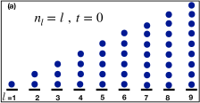
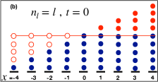
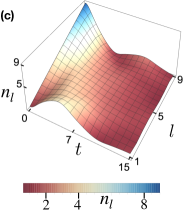
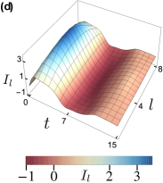
Figure 2: Evolution of a linear chain of Bosons, starting from a Fock state. Each site $l$ is connected to a bath with temperature $T=g$ and chemical potential $\mu_{l}$, where $\mu_{l}=\mu_{1}+\nu(l-1)$ with $\mu_{1}=-4.05g$ and $\nu=0.75g$. Here $g$ is the tunneling amplitude in the linear chain. (a) The initial Fock state in a $N=9$ site system where the $l^{th}$ site is occupied by $l$ particles. Each circle represents a particle. (b) The same Fock state with the origin shifted to the central site and local densities defined in terms of their deviations from the occupation of the central site, i.e $5$. The filled red circles indicate positive deviations while empty red circles indicate negative deviations. In terms of the deviations, the initial profile is anti-symmetric under reflection about the central site. (c) Color-plot of density, $n_{l}(t)$ and (d) current, $I_{l}(t)$ in the system as a function of site (link) number and time in under-damped regime with system bath coupling $\epsilon=0.35g$. The density profile executes a see-saw motion keeping the density of the central site almost constant at short times. The current shows a maximum at the center at short times. At long times, system settles to a density profile decreasing from left to right, governed by the chemical potential gradient in the baths. We use $g=1$ to set the unit of time, $t$ and $l$ is measured in units of lattice spacing.

We now illustrate the potency of this formalism by studying the dynamics of current and density profiles in Fermionic/ Bosonic OQS initialized to specific $\hat{\rho}_{0S}$. We consider a system of Bosons/Fermions hopping on a 1D lattice of $N$ sites with nearest neighbour tunneling amplitude $g$. Each site $l$ of the lattice is coupled to the first site of a semi-infinite 1D Bosonic/Fermionic bath kept at fixed temperature $T_{l}$ and chemical potential $\mu_{l}$ with the same coupling strength $\epsilon$. The baths are modeled by a hopping Hamiltonian with the hopping strength $t_{B}$. The total Hamiltonian of the system ($H_{s}$) , the baths ($H_{b}$) and system bath interaction ($H_{sb}$) are then given by Chakraborty and Sensarma (2018),

$$H_{s} = -g\sum_{l=1}^{N}a_{l}^{\dagger}a_{l+1}+h.c~{}~{}and~{}~{}H_{sb}=\epsilon\sum_{l=1}^{N}a_{l}^{\dagger}b^{(l)}_{1}+h.c$$

$$H_{b} = -t_{B}\sum_{l=1}^{N}\sum_{s=1}^{\infty}b^{(l)\dagger}_{s}b^{(l)}_{s+1}+h.c.$$ (55)

where $a_{l}$ is the annihilation operator (Bosons/Fermions) on the $l^{th}$ site of the system, and $b^{(l)}_{s}$ is the annihilation operator (Bosons/Fermions) of the $s^{th}$ site of the bath connected to $l^{th}$ site of the system. This kind of semi-infinite bath model yields a bath spectral function $\mathcal{J}(\omega)$, which has a square-root derivative singularity at the two band edges, $\omega=\pm 2t_{B}$,

$$\mathcal{J}(\omega)=\Theta(4t_{B}^{2}-\omega^{2})\frac{2}{t_{B}}\sqrt{1-\frac{\omega^{2}}{4t^{2}_{B}}}.$$ (56)

This is a minimal model of non-Markovian dynamics of the OQS induced by non-analyticities in the bath spectral function Chakraborty and Sensarma (2018). The motivation for choosing this model is two-fold: (i) to show that our formalism can easily treat non-Markovian dynamics of OQS and (ii) this is an ideal case to study the effects of the initial condition, since the system retains memories over long timescales.

In this case [Chakraborty and Sensarma, 2018], we have

$$\Sigma^{B}_{R}(\alpha,\beta,\omega)=\delta_{\alpha\beta}\left[\frac{\epsilon^{2}\omega}{2t_{B}^{2}}-\mathbf{i}~{}\frac{\epsilon^{2}}{t_{B}}\left[1-\frac{(\omega+\mathbf{i}\eta)^{2}}{4t_{B}^{2}}\right]^{1/2}\right]$$

and hence the retarded Green’s function is obtained to be,

$${G}_{R}^{O}(\alpha,\beta,\omega)=(-1)^{\alpha+\beta}\frac{M_{\alpha-1}M_{N-\beta}}{gM_{N}}~{}~{}~{}for~{}\alpha<\beta$$

and ${G}_{R}^{O}(\alpha,\beta)={G}_{R}^{O}(\beta,\alpha)$ for $\alpha>\beta$, where

$$M_{\alpha}=\frac{\sinh[(\alpha+1)\lambda]}{\sinh[\lambda]}~{}~{}with~{}~{}\cosh\left[\lambda\right]=\frac{1}{2g}[\omega-\Sigma^{R}(\omega)].$$

From these analytical solutions, we obtain the retarded Green’s functions in time domain by performing the integral in Eq. 52. Finally, the physical Keldysh Green’s functions are obtained by plugging ${G}_{R}^{O}(\alpha,\beta,t-t^{\prime})$ and

$$\Sigma^{B}_{K}(\alpha,\beta,t-t^{\prime}) = -\mathbf{i}\delta_{\alpha,\beta}~{}\epsilon^{2}/2\pi\int d\omega J(\omega)$$

$$\left[\coth(\omega-\mu_{\alpha})/2T_{\alpha}\right]^{\zeta}exp[-\mathbf{i}\omega(t-t^{\prime})]$$

back in eqn. LABEL:gkoqsB, where $\zeta=\pm 1$ for Bosons (Fermions).

The inherent non-Markovianness of the model is manifested as power law kernels, $\sim(t-t^{\prime})^{-3/2}$ in $\Sigma^{B}_{R}(\alpha,\beta,t-t^{\prime})$ and $\Sigma^{B}_{K}(\alpha,\beta,t-t^{\prime})$. This leads to an initial exponential decay in ${G}_{R}^{O}(\alpha,\beta,t-t^{\prime})$, followed by a long time power law tail $\sim(t-t^{\prime})^{-3/2}$, appearing at a time scale $\sim t_{B}/\epsilon^{2}$, which have been explored in great details in Ref [Chakraborty and Sensarma, 2018] .

We first consider a linear chain of Bosons of $N=9$ sites. The system is initialized in a Fock state where the first site has 1 particle, the second site has 2 particles .. the $l^{th}$ site has $l$ particles, as shown in Fig. 2 (a). This creates a positive density gradient from left to right in the initial state. We couple each site to a bath, with the chemical potential $\mu_{l}=\mu_{1}+\nu(l-1)$, keeping the temperature same for all baths. The chemical potential is set up in such a way that in the steady state, the system will have a positive density gradient from right to left, thus ensuring a non-trivial dynamics in this OQS. We choose the system bath coupling strength to be in the under-damped regime, i.e. $\epsilon/g=0.35<1$, so that we can study the interesting transient quantum dynamics of the OQS. The other parameters are chosen to be $t_{B}=2g,T_{l}=g,\mu_{1}=-4.05g$ and $\nu=0.75g$.

The time-dependent density at site $l$ and the current on the link between the sites $l$ and $l+1$ sites are given by, $n_{l}(t)=\zeta[\mathbf{i}{\cal G}^{O}_{K\rho_{0}}(l,t,l,t)-1]/2$ and $I_{l}(t)=g~{}Re[{\cal G}^{O}_{K\rho_{0}}(l,t,l+1,t)]$. The change in the density profile with time is plotted in Fig. 2(c), while the change in current profile along the links of the system is plotted in Fig. 2(d). At short times, we find that the density at the central site, $\bar{n}$ does not change with time, while the profile executes a see-saw type motion with the central site as a fulcrum, i.e. the local density deviation from $\bar{n}$ increases in magnitude with distance from the central site and is antisymmetric under reflection through this point. To understand the short time quantum dynamics of the system, it is enough to consider the dynamics of a closed system with an odd ($2N+1$) number of sites (we will comment on the case of even number of sites later). This description will be valid upto a time scale $\sim t_{B}/\epsilon^{2}$, when the effect of the bath starts to become prominent. In this case, it is useful to set the origin at the central site, and denote the new co-ordinates by $x$ ($-N\leq x\leq N$), so that the Hamiltonian has a reflection symmetry about the origin ($x\rightarrow-x$). Further we consider the deviation of the density from $\bar{n}$, $\delta n_{x}(t)$. The initial profile $\delta n_{x}(0)$ is antisymmetric under reflection. This is shown in Fig. 2(c) in terms of open (negative $\delta n_{x}(0)$) and filled (positive $\delta n_{x}(0)$) red circles. Probability conservation implies that $\sum_{y}|G^{R}(x,t;y,0)|^{2}=1$. Using this we get,

$$\delta n_{x}(t)=\sum_{y}|G^{R}(x,t;y,0)|^{2}\delta n_{y}(0)$$ (57)

Here the retarded Green’s function $G^{R}$ does not depend on the initial conditions and exhibits the reflection symmetry of the Hamiltonian, i.e. $G^{R}(x,t;y,0)=G^{R}(-x,t;-y,0)$, while $\delta n_{-y}(0)=-\delta n_{y}(0)$. It is then easy to see that $\delta n_{x}(t)$ is antisymmetric under reflection, and hence $\delta n_{x}(t)$ is $0$ for the central site ($x=0$). This leads to a piling up of current in the middle at shown in figure 2(d). The maximum of the current at the center can be understood from the continuity equation $\partial n/\partial t\sim\nabla.\vec{j}$.We can get further insight for a large system, where the boundaries can be neglected. In this case, $|G^{R}(x,t,y,0)|^{2}$ is a function of $|x-y|$, and using the anti-symmetry of the initial profile, it can be shown that $\delta n_{x}(t)\sim x$, i.e it increases in magnitude linearly with the distance from the central site. In presence of a series of baths with a chemical potential gradient, the reflection symmetry is broken, and at long times $\sim t_{B}/\epsilon^{2}$, the system gradually settles down to a steady state behaviour. Note that for a system with even number of sites, the reflection symmetry is about the center of a link. Sites at the two ends of this central link will have a small but non-zero change in density with mutually opposite signs at short times.

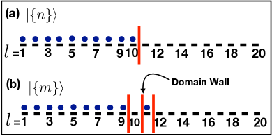
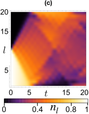
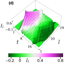
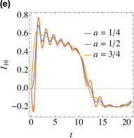
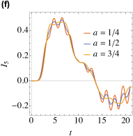
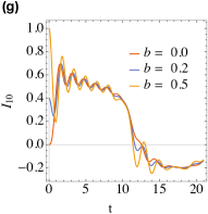
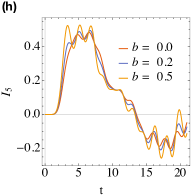
Figure 3: Dynamics of a Fermionic OQS starting from arbitrary initial condition. A $20$ site linear chain of spinless Fermions with nearest neighbour tunneling amplitude $g$ is coupled at each site to the baths at temperature $T_{l}=g$ and the chemical potential $\mu_{l}=-4.05g$ through a coupling $\epsilon=0.2g$. (a) The initial state $|\{n\}\rangle$, with left half occupied, the right half empty and a domain wall at the center. (b) Another initial state $|\{m\}\rangle$, obtained from moving the rightmost particle in $|\{n\}\rangle$, one site to its right. Color plot of (c) for density and (d) for current as a function of site (link) number and time for a system starting with $|\{n\}\rangle\langle\{n\}|$. The diamonds are defined by ballistic motion of domain walls and their reflection from the edges. (e)-(h) Current as a function of time for off-diagonal $\hat{\rho}_{0S}=a\left|\left\{n\right\}\right\rangle\left\langle\left\{n\right\}\right|+\left(1-a\right)\left|\left\{m\right\}\right\rangle\left\langle\left\{m\right\}\right|+[\mathbf{i}b\left|\left\{n\right\}\right\rangle\left\langle\left\{m\right\}\right|+h.c.]$. (e) Current at the central link ($l=10$) for $b=0$ and $a=1/4,1/2,3/4$. (f) Same as (e) for a link far from the center ($l=5$). The initial oscillations at the central link are more pronounced for smaller $a$. (g) Current at the central link ($l=10$) and (h) current at the link far from the center $l=5$ for $\hat{\rho}_{0S}$ with $a=1/2$ and $b=0.0,0.2,0.5$. The initial current on the central link is controlled by the value of $b$. We use $g=1$ to set the unit of time, $t$ and $l$ is measured in units of lattice spacing.

We next consider spinless Fermions hopping on a 1D lattice of $N=20$ sites. We first consider an initial Fock state, where the left half of the lattice (sites $1$ to $10$) is occupied by particles, while the right half of the system is empty, creating a domain wall in the middle of the lattice, as shown in Fig 3 (a). The Fermionic bath parameters are fixed to $T_{l}=g$ and $\mu_{l}=-4.05g$ and $\epsilon=0.2g$, i.e there is no inhomogeneity in the bath parameters. At short times, the effect of the bath can be ignored and the quantum dynamics can be understood by considering the domain wall as a free particle. This particle splits coherently and moves in either direction ballistically with a timescale $\sim g^{-1}$. The effect is seen both in the changes in the density profile ( Fig. 3 (c) ) and in the current profile (Fig. 3 (d)), which shows a sudden jump at a site when the particle first passes through that site, creating the initial wedge shaped profiles. The particle is coherently reflected back at the boundary and rephases at a single point  Preiss et al. (2015), creating the diamond shape in the profile. Since the system is underdamped, this cycle is repeated with associated sign change in the current profile, as seen in Fig. 3 (d). Beyond the time scale $\sim t_{B}/\epsilon^{2}$, the presence of the bath governs the dynamics; here the current goes to zero and the density profile attains its steady uniform value dictated by the chemical potential in the bath at long times, but the approach to the steady state is governed by the power law of the non-Markovian bath.

We now consider the same Fermionic system initialized to a different density matrix. We consider 2 Fock states, with one state given by the domain wall profile shown in Fig. 3 (a) (i.e. the initial state with the domain wall at the center). The second state is obtained from this state by hopping the particle at site $10$ to the site $11$, resulting in a configuration shown in Fig. 3 (b). Let us call these states $|\left\{n\right\}\rangle$ and $|\left\{m\right\}\rangle$ respectively. We will consider a general $2\times 2$ initial density matrix in the qubit space, spanned by these two states of the form, $\hat{\rho}_{0S}=a\left|\left\{n\right\}\right\rangle\left\langle\left\{n\right\}\right|+\left(1-a\right)\left|\left\{m\right\}\right\rangle\left\langle\left\{m\right\}\right|+[\mathbf{i}b\left|\left\{n\right\}\right\rangle\left\langle\left\{m\right\}\right|+h.c.]$. We note that the positivity of the eigenvalues of $\hat{\rho}_{0S}$ demands $\left|b\right|^{2}\leq a\left(1-a\right)$. When $b$ is finite, the system has a non-zero current on the central link. We first consider the system with $b=0$, and plot the current on the central link as a function of time in Fig 3 (e). In this case, the current is initially expected to rise for $a>1/2$, since there is more density at $l=10$ than at $l=11$, and to fall in value for $a<1/2$ (note that the current from right to left is considered to be positive in our notation). This is indeed observed as $a$ is varied from $1/4$ to $3/4$ in Fig. 3 (e). We note that the amplitude of the oscillations of the current decreases with increases in $a$. In Fig. 3 (f), we plot the current at a link $l=5$ far from the center. We see that the current rises after a finite time, as discussed in the previous case. We also find that changing $a$ from $1/2$ to $3/4$ causes minor changes in the current, i.e. the changes in the initial conditions mainly affect the dynamics in the center of the lattice.

We now consider an off-diagonal $\hat{\rho}_{0S}$ with $a$ fixed to $1/2$, and change $b$ from $0$ to $1/2$. The current in the central link is plotted in Fig. 3 (g), while the current in the link far away $(l=5)$ is plotted in Fig. 3 (h). The key difference in seen in Fig. 3 (g), where the current in the central link starts from a finite value, governed by $b$. The subsequent dynamics is almost independent of $b$ in all cases.

VII Interacting Systems

In the previous sections, we have built up a field theoretic formalism to describe the dynamics of quantum many body systems starting from arbitrary initial conditions. We have also extended this formalism to the case of open quantum systems. However, till now, we have only looked at non-interacting systems (quadratic or gaussian field theories), where we can solve the problem exactly and the question of calculating a correlator is reduced to evaluating one or a few integrals. In this section we finally tackle the question of applying our formalism to the dynamics of interacting quantum many body systems starting from an arbitrary initial condition.

In this case, we start by adding to the quadratic Keldysh action with the initial bilinear source, $S(u)$, a term $S_{int}$, representing the interaction between particles. We then consider the field theory controlled by the action $S=S(u)+S_{int}$, and calculate Green’s functions $\hat{G}^{(n)}_{int}(u)$ in this theory. $\hat{G}^{(n)}_{int}(u)$ has a diagrammatic expansion in terms of the non-interacting Green’s functions $\hat{G}(u)$ and the interaction vertices of a standard SK field theory. The details of this construction depends on the form of $S_{int}$, but the Feynman rules for computing the diagrams are exactly similar to that of a SK field theory, with $u$ dependent propagators $\hat{G}(u)$.

The diagrammatic perturbation theory for the Green’s functions work well at short times, but one needs to resum the series or part of it to all orders to obtain an accurate description of the long time behaviour. This is a general characteristics of perturbation theories and has nothing to do with arbitrary initial conditions. This is where our formalism has an advantage: the standard resummation techniques known in field theories apply to $G^{(n)}_{int}(u)$, while they do not apply to the physical correlators ${\cal G}^{(n)}_{int,\rho_{0}}={\cal L}(\partial_{u},\rho_{0}){\cal N}(u)G^{(n)}_{int}(u)|_{u=0}$. Focusing on the one-particle Green’s function, one can now write a Dyson equation $\hat{G}_{int}(u)=[G^{-1}(u)-\Sigma(G(u))]^{-1}$, where the irreducible self energy can be constructed diagrammatically in perturbation theory. One can also use a skeleton expansion in terms of $\Sigma(G_{int}(u))$, or resum a class of diagrams as in a RPA expansion; in other words one can bring the full force of accumulated knowledge of such approximation schemes to bear down on the problem of calculating $\hat{G}_{int}(u)$. Similar constructions are possible for higher order correlation functions in terms of higher order vertex functions.

We will not go into any particular approximation in this paper since the validity of different approximations are both model dependent and parameter dependent. We will take this up in a future work. It may seem that applying a large number of derivatives (equal to number of particles) through ${\cal L}$ will be a daunting task in the case of thermodynamically large interacting systems, specially for resumed approximations, where $G_{int}(u)$ may only be known approximately, or even numerically. We will not provide a complete solution to this problem here, but indicate a way forward. We will consider the system to initially be in a single Fock state. The generalization to arbitrary density matrices can be done suitably. For a Fermionic system, starting in a Fock state $|\{n\}\rangle$, where the set of occupied modes are denoted by ${\cal A}$, we can write

$${\cal G}_{\rho_{0}}=\prod_{\alpha\in{\cal A}}[1+\partial_{u_{\alpha}}]G(u)|_{u=0} = G(0)+\sum_{\alpha\in{\cal A}}G^{\alpha}(0)$$

$$+ \frac{1}{2!}\sum_{\alpha\beta\in{\cal A},\alpha\neq\beta}G^{\alpha\beta}(0)+...$$

where $G^{ijk....n}=\partial_{u_{i}}...\partial_{u_{n}}G(u)$. For a Bosonic system, a similar derivative expansion can be written as

$${\cal G}_{\rho_{0}}=\prod_{\alpha}\sum_{m=0}^{n_{\alpha}}\frac{\partial^{m}_{u_{\alpha}}}{m!}G(u)|_{u=0}=G(0)+\sum_{\alpha\in{\cal A}}G^{\alpha}(0)+...$$ (59)

where ${\cal A}$ is the set of modes with at least $1$ particles. For a thermodynamically large system, there are two possible practical approximations to treat the derivative expansion: (i) truncate the series or (ii) resum this series by assuming factorization of correlation functions of higher order. We will not go into the relative merits of these different approximation strategies, and leave this as a topic of future studies on this subject.

VIII Conclusion

In this paper, we have formulated a field theoretic description of dynamics of a quantum many body system (Bosons and Fermions) starting from an arbitrary initial density matrix. We have shown that the matrix element of the density matrix can be incorporated using a source which couples to the bilinears of the fields only at initial time, i.e by adding an impulse term to the original SK action. The Green’s functions can be evaluated in this theory as a function of the addition source $\hat{u}$. The physical correlation functions can then be obtained by taking an appropriate set of derivatives of the Green’s functions w.r.t the initial source and setting the sources to zero. The initial density matrix only governs the particular set of derivatives to be taken. Our formalism thus breaks up into two parts: (i) calculation of Green’s functions in presence of a bilinear source, where the hierarchy of Green’s functions satisfy Wick’s theorem and the standard SK field theoretic techniques can applied to compute them, (ii) taking a particular set of derivatives, which depend on the initial conditions. We extend this formalism to open quantum systems and calculate evolution of density and current profile in Bosonic and Fermionic OQS. We calculate the exact expressions for physical one-particle and two-particle correlators in a non-interacting system and characterize the violation of Wick’s theorem, relating it to the connected to particle correlations in the initial state. We have briefly sketched how our formalism can be extended to interacting systems. The biggest challenge that we have not addressed here are strategies to obtain reasonable approximation schemes which are controlled in particular limits. The issue of making conserving approximations which are valid at long times (i.e. no perturbation theory for physical correlators) is one of great importance which we hope to address in a future work.

Appendix A Calculation of $\mathcal{N}(u)$ and $\hat{G}(u)$ for the diagonal initial density matrix

An important step in the formalism we have developed for a quantum many body system starting from $\hat{\rho}_{0}=\sum_{\{n\}}c_{\{n\}}|\{n\}\rangle\langle\{n\}|$ is to invert the kernel $\hat{G}^{-1}(\alpha,t,\beta,t^{\prime},\vec{u})$ in the inverse Green’s function analytically and obtain the closed form expression for the $\vec{u}$ dependent normalization, $\mathcal{N}(u)=Det[-\mathbf{i}\hat{G}^{-1}(u)]^{-\zeta}$ and also the Green’s function, $\hat{G}(u)$ with the initial source $\vec{u}$, as they serve as the building blocks for the further steps of the many body formalism. In this appendix, we will work out the structure of calculating $\mathcal{N}(u)$ and $\hat{G}(u)$ from $\hat{G}^{-1}(\alpha,t,\beta,t^{\prime},\vec{u})$ for a many body Bosonic system.

To construct these objects, it is useful to isolate the $\vec{u}$ dependent part in the action from the from part independent of the initial condition to write,

$$\hat{G}^{-1}(u_{\alpha})=\hat{G}^{-1}(0)-\hat{\Delta}(u_{\alpha})$$ (60)

where $\hat{G}^{-1}(0)=\hat{G}^{-1}(\alpha,t;\beta,t^{\prime})|_{\vec{u}=0}$ is the two component inverse Green’s function when the system starts in the vacuum state, and is obtained by setting $u_{\alpha}=0$. It is evident from the text below equation 18 of the main text, that the $\vec{u}$ dependent part $\Delta$ is finite only for the $+-$ component, i.e.

$$\Delta_{++}=\Delta_{--}=\Delta_{-+}=0~{},~{}\Delta_{+-}(\alpha,t;\beta,t^{\prime},\vec{u})=\mathbf{i}\delta_{\alpha\beta}\delta_{t}\delta_{t^{\prime}}u_{\alpha}.$$ (61)

Now, we will write,

$$Det[-\mathbf{i}\hat{G}^{-1}(\vec{u})]=e^{Tr[\log\{-\mathbf{i}\hat{G}^{-1}(\vec{u})\}]}$$

which leads to,

$$Tr[\log\{-\mathbf{i}\hat{G}^{-1}(\vec{u})\}] = Tr[\log\{-\mathbf{i}\hat{G}^{-1}(0)\}]+Tr[\log\{1-\hat{G}(0)\hat{\Delta}(\vec{u})\}]$$ (62)

$$= Tr[\log\{-\mathbf{i}\hat{G}^{-1}(0)\}]-Tr\left[\hat{G}(0)\hat{\Delta}(\vec{u})+\frac{1}{2}\hat{G}(0)\hat{\Delta}(\vec{u})\hat{G}(0)\hat{\Delta}(\vec{u})+..\right]$$

where,

$$Tr\left[\hat{G}(0)\hat{\Delta}(\vec{u})\right] = Tr\left[\hat{G}_{-+}(0)\hat{\Delta}_{+-}(\vec{u})\right]=\mathbf{i}\sum\limits_{\alpha}G_{-+}(\alpha,0;\beta,0;0)u_{\alpha}=\sum\limits_{\alpha}u_{\alpha}.$$ (63)

Here the vacuum Green’s functions $\hat{G}(0)=\hat{G}^{v}$are given by

$$G_{-+}^{v}(\alpha,t;\beta,t^{\prime}) = -\mathbf{i}\sum_{a}\psi^{\ast}_{a}(\beta)\psi_{a}(\alpha)e^{-iE_{a}(t-t^{\prime})}~{},~{}G_{+-}^{v}(\alpha,t;\beta,t^{\prime})=0,$$

$$G_{++}^{v}(\alpha,t;\beta,t^{\prime}) = \Theta(t-t^{\prime})G_{-+}^{v}(\alpha,t;\beta,t^{\prime})~{},~{}and~{}G_{--}^{v}(\alpha,t;\beta,t^{\prime})=\Theta(t^{\prime}-t)G_{-+}^{v}(\alpha,t;\beta,t^{\prime}),$$ (64)

where $E_{a}$ are the eigenvalues and $\psi_{a}(\alpha)$ are the corresponding eigenvectors of the Hamiltonian of the multimode system. Using the orthogonality property of eigenmodes we get, $\mathbf{i}G_{-+}(\alpha,0;\beta,0;0)=\delta_{\alpha,\beta}$ at the initial time $t=t^{\prime}=0$, Similarly,

$$Tr\left[\hat{G}(0)\hat{\Delta}(\vec{u})\hat{G}(0)\hat{\Delta}(\vec{u})\right] = \frac{1}{2}Tr\left[\hat{G}_{-+}(\alpha,0;\beta,0;0)\mathbf{i}u_{\beta}\hat{G}_{-+}(\beta,0;\gamma,0;0)\mathbf{i}u_{\gamma}\right]=\frac{1}{2}\sum\limits_{\alpha}u^{2}_{\alpha}.$$ (65)

Using similar argument for all terms in the expansion (equation 62) and adding them up, we obtain,

$$Tr[\log\{-\mathbf{i}\hat{G}^{-1}(\vec{u})\}] = Tr[\log\{-\mathbf{i}\hat{G}^{-1}(0)\}]+\sum\limits_{\alpha}\log\left(1-u_{\alpha}\right)$$

$$Det[-\mathbf{i}G^{-1}] = Det[-\mathbf{i}G^{-1}(0)]\prod_{\alpha}1-u_{\alpha}$$ (66)

which is quoted in equation 19 in the main text.

Now, we will show how to invert the kernel $\hat{G}^{-1}(u)$ to obtain closed form answer for $\hat{G}(u)$. We have,

$$\hat{G}(\vec{u})=\left[\hat{G}^{-1}(0)-\hat{\Delta}(u_{\alpha})\right]^{-1}=\hat{G}(0)\left[1-\hat{G}(0)\hat{\Delta}(u_{\alpha})\right]^{-1}$$

$$=\hat{G}(0)+\hat{G}(0)\hat{\Delta}(u_{\alpha})\hat{G}(0)+\hat{G}(0)\hat{\Delta}(u_{\alpha})\hat{G}(0)\hat{\Delta}(u_{\alpha})\hat{G}(0)+...$$

We will show here the structure of the above sum for one of the components, say $G_{++}(\alpha,t;\beta,t^{\prime};\vec{u})$. The expansion of $\hat{G}_{++}(\vec{u})$ can be written as,

$$G_{++}(\alpha,t;\beta,t^{\prime};\vec{u}) = G_{++}^{v}(\alpha,t;\beta,t^{\prime})+\mathbf{i}\sum\limits_{\gamma}G_{++}^{v}(\alpha,t;\gamma,0)u_{\gamma}G_{-+}^{v}(\gamma,0;\beta,t^{\prime})$$ (67)

$$+ \mathbf{i}^{2}\sum\limits_{\gamma,\kappa}G_{++}^{v}(\alpha,t;\gamma,0)u_{\gamma}G_{-+}^{v}(\gamma,0;\kappa,0)u_{\kappa}G_{-+}^{v}(\kappa,0;\beta,t^{\prime})+..$$

$$= G_{++}^{v}(\alpha,t;\beta,t^{\prime})+\mathbf{i}\sum\limits_{\gamma}G_{++}^{v}(\alpha,t;\gamma,0)u_{\gamma}G_{-+}^{v}(\gamma,0;\beta,t^{\prime})+\mathbf{i}\sum\limits_{\gamma}G_{++}^{v}(\alpha,t;\gamma,0)u_{\gamma}^{2}G_{-+}^{v}(\gamma,0;\beta,t^{\prime})$$

$$= G_{++}^{v}(\alpha,t;\beta,t^{\prime})+\mathbf{i}\sum\limits_{\gamma}\frac{u_{\gamma}}{1-u_{\gamma}}G_{++}^{v}(\alpha,t;\gamma,0)G_{-+}^{v}(\gamma,0;\beta,t^{\prime})$$

Similar arguments will apply to the other components as well which will lead to equation for $G_{\mu\nu}(\alpha,t;\beta,t^{\prime};\vec{u})$ in the main text.

Appendix B Generic density matrix

Green’s functions

The physical Green’s function is given by

$${\cal G}^{\rho}=\sum_{nm}\frac{c_{nm}}{\prod_{\alpha}\sqrt{n_{\alpha}!m_{\alpha}!}}\left.\prod_{i}[\partial_{\alpha_{i}\beta_{i}}]Z[0,\hat{u}]G(\hat{u})\right|_{\hat{u}=0},$$ (68)

where $G(\hat{u})$ is given by eqn. 25. The first term in $G(\hat{u})$, the vacuum Green’s function part, is independent of $\hat{u}$ and the just goes out of the above derivatives. For the second term, we need to evaluate

$$\sum_{nm}\frac{c_{nm}}{\prod_{\alpha}\sqrt{n_{\alpha}!m_{\alpha}!}}\left.\prod_{i}[\partial_{\alpha_{i}\beta_{i}}]\frac{[(1-\hat{u})^{-1}-1]_{\gamma\delta}}{\det(1-\hat{u})^{-1}}\right|_{\hat{u}=0}.$$ (69)

We shall calculate the derivatives below. Again defining $A=1-\hat{u}$, we have

$$d_{N}\cdots d_{1}\left(A^{-1}\det A^{-1}\right) =A^{-1}d_{N}d_{N-1}\cdots d_{2}d_{1}\det A^{-1}$$

$$\ \ \ +d_{1}A^{-1}d_{N}d_{N-1}\cdots d_{2}\det A^{-1}+d_{2}A^{-1}d_{N}d_{N-1}\cdots d_{3}d_{1}\det A^{-1}+\cdots$$

$$\ \ \ +d_{2}d_{1}A^{-1}d_{N}d_{N-1}\cdots d_{3}\det A^{-1}+d_{3}d_{1}A^{-1}d_{N}d_{N-1}\cdots d_{4}d_{2}\det A^{-1}+\cdots$$

$$\ \ \ +d_{3}d_{2}d_{1}A^{-1}d_{N}d_{N-1}\cdots d_{4}\det A^{-1}+\cdots$$

$$\ \ \ +\cdots+d_{N}d_{N-1}\cdots d_{2}d_{1}A^{-1}\det A^{-1}.$$ (70)

After substituting $\hat{u}=0$, the first line of eqn. 70 gives

$$\left.[A^{-1}]_{\gamma\delta}\prod_{i}[\partial_{\alpha_{i}\beta_{i}}]\det A^{-1}\right|_{\hat{u}=0}=\delta_{\gamma\delta}\langle\{m\}|\{n\}\rangle\prod_{\alpha}n_{\alpha}!\ .$$ (71)

which cancels the contribution from $[-1]_{\gamma\delta}$ part in eqn. 25 exactly. To get an intuition for how to deal with the rest of the terms, let us focus on the first term in the second line of eqn. 70,

$$\left.[\partial_{\alpha_{1}\beta_{1}}A^{-1}]_{\gamma\delta}\prod_{i\neq 1}[\partial_{\alpha_{i}\beta_{i}}]\det A^{-1}\right|_{\hat{u}=0}=\delta_{\gamma\alpha_{1}}\delta_{\beta_{1}\delta}\sum_{P}\langle P(\vec{\beta})|\vec{\alpha}\rangle.$$ (72)

where $P$ is now understood to be a permutation on $N$ labels that fixes $\beta_{1}$, that is, $P(\beta_{1})=\beta_{1}$, and the matrix element has only $\alpha_{i}$’s and $\beta_{i}$’s for $i=2,\ldots,N$. The other terms in the sum can now be determined using the symmetry arguments using before in calculating the partition function. We could start our analysis with the states $|\alpha^{\prime}_{1}\cdots\alpha^{\prime}_{N}\rangle=|Q(\alpha_{1})\cdots Q(\alpha_{N})\rangle$ and $|\beta^{\prime}_{1}\cdots\beta^{\prime}_{N}\rangle=|R(\beta_{1})\cdots R(\beta_{N})\rangle$, where $Q$ and $R$ any permutations, because nothing physical depends on this choice. Using these new labels, the above equation would give us

$$\left.[\partial_{\alpha^{\prime}_{1}\beta^{\prime}_{1}}A^{-1}]_{\gamma\delta}\prod_{i\neq 1}[\partial_{\alpha^{\prime}_{i}\beta^{\prime}_{i}}]\det A^{-1}\right|_{\hat{u}=0}=\delta_{\gamma\alpha^{\prime}_{1}}\delta_{\beta^{\prime}_{1}\delta}\sum_{P}\langle P(\vec{\beta}^{\prime})|\vec{\alpha}^{\prime}\rangle=\delta_{\gamma\alpha_{k}}\delta_{\beta_{l}\delta}\sum_{P}\langle P(Q(\vec{\beta}))|R(\vec{\alpha})\rangle=\delta_{\gamma\alpha_{k}}\delta_{\beta_{l}\delta}\sum_{P}\langle P(\vec{\beta})|\vec{\alpha}\rangle,$$ (73)

where, there exist $k$ and $l$ such that $Q(\alpha_{1})=\alpha_{k}$, $R(\beta_{1})=\beta_{l}$, and the vectors $\vec{\alpha}$ and $\vec{\beta}$ do not contain $\alpha_{k}$ and $\beta_{l}$ respectively. Also, $P$ runs over all permutations that fix $\beta_{l}$.

It is not hard to convince oneself that all the terms in eqn. 70 are of the above form for different choices of $Q$ and $R$. For example, the second term in the second line, $d_{2}A^{-1}d_{N}d_{N-1}\cdots d_{3}d_{1}\det A^{-1}$, corresponds to $k=l=2$, whereas the sum

$$= d_{2}d_{1}A^{-1}d_{N}\cdots d_{3}\det A^{-1}+d_{2}d_{3}d_{1}A^{-1}d_{N}\cdots d_{4}\det A^{-1}+d_{2}d_{4}d_{1}A^{-1}d_{N}\cdots d_{5}d_{3}\det A^{-1}+\cdots$$

$$+\ d_{2}d_{3}d_{4}d_{1}A^{-1}d_{N}\cdots d_{5}\det A^{-1}+d_{2}d_{3}d_{5}d_{1}A^{-1}d_{N}\cdots d_{6}d_{4}\det A^{-1}+d_{2}d_{4}d_{5}d_{1}A^{-1}d_{N}\cdots d_{6}d_{3}\det A^{-1}+\cdots,$$

[that is, the sum of all terms with $d_{1}$ and $d_{2}$ being the first and last derivatives to act on $A^{-1}$] corresponds to $k=2$ and $l=1$. Hence, the LHS of eqn. 70 reduces to the following expression in occupation number basis,

$$\prod_{i}[\partial_{\alpha_{i}\beta_{i}}]\frac{[A^{-1}-1]_{\gamma\delta}}{\det A} =\sum_{kl}\delta_{\gamma\alpha_{k}}\delta_{\beta_{l}\delta}\sum_{P}\langle P(\vec{\beta})|\vec{\alpha}\rangle=\sum_{P}\langle P(\vec{\beta})|\hat{a}^{\dagger}_{\delta}\hat{a}_{\gamma}|\vec{\alpha}\rangle=\langle\{m\}|\hat{a}^{\dagger}_{\delta}\hat{a}_{\gamma}|\{n\}\rangle\prod_{\gamma}\sqrt{n_{\gamma}!m_{\gamma}!}\ .$$ (75)

The expression in eqn. 69 can then be written as an expectation value in the initial density matrix,

$$\sum_{nm}\frac{c_{nm}}{\prod_{\alpha}\sqrt{n_{\alpha}!m_{\alpha}!}}\left.\prod_{i}[\partial_{\alpha_{i}\beta_{i}}]\frac{[(1-\hat{u})^{-1}-1]_{\gamma\delta}}{\det(1-\hat{u})^{-1}}\right|_{\hat{u}=0}=\sum_{nm}c_{nm}\langle\{m\}|\hat{a}^{\dagger}_{\delta}\hat{a}_{\gamma}|\{n\}\rangle=\text{tr}(\hat{\rho}_{0}\hat{a}^{\dagger}_{\delta}\hat{a}_{\gamma})\equiv\langle\hat{a}^{\dagger}_{\delta}\hat{a}_{\gamma}\rangle_{0}.$$ (76)

Substituting this result into eqn. 68 gives the physical Green’s functions in the main text,

$${\cal G}_{K\rho_{0}}(\alpha,t;\beta,t^{\prime})=-\mathbf{i}\sum_{\gamma\delta}G^{v}_{R}(\alpha,t;\gamma,0)[2\langle\hat{a}_{\delta}^{\dagger}\hat{a}_{\gamma}\rangle_{0}+\delta_{\gamma\delta}]G^{v}_{A}(\delta,0;\beta,t^{\prime}).$$ (77)

References

- Eisert et al. (2010) J. Eisert, M. Cramer, and M. B. Plenio, Rev. Mod. Phys. 82, 277 (2010).
- Breuer and Petruccione (2002) H.-P. Breuer and F. Petruccione, The theory of open quantum systems (Oxford University Press on Demand, 2002).
- Agarwal (1969) G. S. Agarwal, Phys. Rev. 178, 2025 (1969).
- Nakajima (1958) S. Nakajima, Progress of Theoretical Physics 20, 948 (1958).
- Zwanzig (1960) R. Zwanzig, The Journal of Chemical Physics 33, 1338 (1960).
- de Vega and Alonso (2017) I. de Vega and D. Alonso, Rev. Mod. Phys. 89, 015001 (2017).
- Zhang et al. (2012) W.-M. Zhang, P.-Y. Lo, H.-N. Xiong, M. W.-Y. Tu, and F. Nori, Phys. Rev. Lett. 109, 170402 (2012).
- Chakraborty and Sensarma (2018) A. Chakraborty and R. Sensarma, Phys. Rev. B 97, 104306 (2018).
- Schollwöck (2011) U. Schollwöck, Annals of Physics 326, 96 (2011), january 2011 Special Issue.
- Eisert (2013) J. Eisert, in Autumn School on Correlated Electrons: Emergent Phenomena in Correlated Matter Jülich, Germany, 23-27. September 2013 (2013) arXiv:1308.3318 [quant-ph] .
- Evenbly and Vidal (2015) G. Evenbly and G. Vidal, Phys. Rev. Lett. 115, 180405 (2015).
- Stoudenmire and White (2012) E. Stoudenmire and S. R. White, Annual Review of Condensed Matter Physics 3, 111 (2012), https://doi.org/10.1146/annurev-conmatphys-020911-125018 .
- Xiang et al. (2001) T. Xiang, J. Lou, and Z. Su, Phys. Rev. B 64, 104414 (2001).
- Altland and Simons (2010) A. Altland and B. D. Simons, Condensed matter field theory (Cambridge University Press, 2010).
- Keldysh (1965) L. Keldysh, JETP 20, 1018 (1965).
- Kamenev and Levchenko (2009) A. Kamenev and A. Levchenko, Advances in Physics 58, 197 (2009).
- Rammer (2007) J. Rammer, Quantum Field Theory of Non-equilibrium States (Cambridge University Press, 2007).
- Kamenev (2011) A. Kamenev, Field theory of non-equilibrium systems (Cambridge University Press, 2011).
- Kadanoff (1962) G. Kadanoff, Leo P./Baym, Quantum Statistical Mechanics (Frontiers in Physics Series by W.A. Benjamin, Inc., 1962).
- Aron et al. (2018) C. Aron, G. Biroli, and L. F. Cugliandolo, SciPost Phys. 4, 008 (2018).
- Jauho et al. (1994) A.-P. Jauho, N. S. Wingreen, and Y. Meir, Phys. Rev. B 50, 5528 (1994).
- Nielsen and Chuang (2010) M. A. Nielsen and I. L. Chuang, Quantum Computation and Quantum Information: 10th Anniversary Edition (Cambridge University Press, 2010).
- Hoover (1999) W. G. Hoover, Time Reversibility, Computer Simulation, and Chaos, Vol. 13 (1999).
- Jensen (1992) R. V. Jensen, Nature 355, 311 EP (1992).
- Rigol (2009) M. Rigol, Phys. Rev. Lett. 103, 100403 (2009).
- Langen et al. (2015) T. Langen, S. Erne, R. Geiger, B. Rauer, T. Schweigler, M. Kuhnert, W. Rohringer, I. E. Mazets, T. Gasenzer, and J. Schmiedmayer, Science 348, 207 (2015), http://science.sciencemag.org/content/348/6231/207.full.pdf .
- Nandkishore and Huse (2015) R. Nandkishore and D. A. Huse, Annual Review of Condensed Matter Physics 6, 15 (2015), https://doi.org/10.1146/annurev-conmatphys-031214-014726 .
- Schreiber et al. (2015) M. Schreiber, S. S. Hodgman, P. Bordia, H. P. Lüschen, M. H. Fischer, R. Vosk, E. Altman, U. Schneider, and I. Bloch, Science 349, 842 (2015), http://science.sciencemag.org/content/349/6250/842.full.pdf .
- Choi et al. (2016) J.-y. Choi, S. Hild, J. Zeiher, P. Schauß, A. Rubio-Abadal, T. Yefsah, V. Khemani, D. A. Huse, I. Bloch, and C. Gross, Science 352, 1547 (2016), http://science.sciencemag.org/content/352/6293/1547.full.pdf .
- Basko et al. (2006) D. Basko, I. Aleiner, and B. Altshuler, Annals of Physics 321, 1126 (2006).
- Labouvie et al. (2016) R. Labouvie, B. Santra, S. Heun, and H. Ott, Phys. Rev. Lett. 116, 235302 (2016).
- Yu et al. (2016) Z. Yu, G.-M. Tang, and J. Wang, Phys. Rev. B 93, 195419 (2016).
- Myöhänen et al. (2009) P. Myöhänen, A. Stan, G. Stefanucci, and R. van Leeuwen, Phys. Rev. B 80, 115107 (2009).
- Jin et al. (2010) J. Jin, M. W.-Y. Tu, W.-M. Zhang, and Y. Yan, New Journal of Physics 12, 083013 (2010).
- Zhou et al. (2016) C. Zhou, X. Chen, and H. Guo, Phys. Rev. B 94, 075426 (2016).
- Myöhänen et al. (2008) P. Myöhänen, A. Stan, G. Stefanucci, and R. van Leeuwen, EPL (Europhysics Letters) 84, 67001 (2008).
- Maciejko et al. (2006) J. Maciejko, J. Wang, and H. Guo, Phys. Rev. B 74, 085324 (2006).
- Yang and Zhang (2016) P.-Y. Yang and W.-M. Zhang, Frontiers of Physics 12, 127204 (2016).
- Karlsson et al. (2018) D. Karlsson, R. van Leeuwen, E. Perfetto, and G. Stefanucci, Phys. Rev. B 98, 115148 (2018).
- Esposito et al. (2009) M. Esposito, U. Harbola, and S. Mukamel, Rev. Mod. Phys. 81, 1665 (2009).
- Tang and Wang (2014) G.-M. Tang and J. Wang, Phys. Rev. B 90, 195422 (2014).
- Tang et al. (2014) G.-M. Tang, F. Xu, and J. Wang, Phys. Rev. B 89, 205310 (2014).
- Cugliandolo et al. (2006) L. F. Cugliandolo, T. Giamarchi, and P. L. Doussal, Phys. Rev. Lett. 96, 217203 (2006).
- Kennett et al. (2001) M. P. Kennett, C. Chamon, and J. Ye, Phys. Rev. B 64, 224408 (2001).
- Halimeh et al. (2018) J. C. Halimeh, M. Punk, and F. Piazza, Phys. Rev. B 98, 045111 (2018).
- Baym and Kadanoff (1961) G. Baym and L. P. Kadanoff, Phys. Rev. 124, 287 (1961).
- Semkat et al. (1999) D. Semkat, D. Kremp, and M. Bonitz, Phys. Rev. E 59, 1557 (1999).
- Semkat et al. (2000) D. Semkat, D. Kremp, and M. Bonitz, Journal of Mathematical Physics 41, 7458 (2000), https://doi.org/10.1063/1.1286204 .
- Yang et al. (2014) P.-Y. Yang, C.-Y. Lin, and W.-M. Zhang, Phys. Rev. B 89, 115411 (2014).
- Yang et al. (2015) P.-Y. Yang, C.-Y. Lin, and W.-M. Zhang, Phys. Rev. B 92, 165403 (2015).
- van Leeuwen and Stefanucci (2012) R. van Leeuwen and G. Stefanucci, Phys. Rev. B 85, 115119 (2012).
- KONSTANTINOV and PEREL (1961) O. V. KONSTANTINOV and V. I. PEREL, JETP 12, 142 (1961).
- Wagner (1991) M. Wagner, Phys. Rev. B 44, 6104 (1991).
- Leeuwen and Stefanucci (2013) R. v. Leeuwen and G. Stefanucci, Journal of Physics: Conference Series 427, 012001 (2013).
- Garny and Müller (2009) M. Garny and M. M. Müller, Phys. Rev. D 80, 085011 (2009).
- Sieberer et al. (2014) L. M. Sieberer, S. D. Huber, E. Altman, and S. Diehl, Phys. Rev. B 89, 134310 (2014).
- Sarkar et al. (2014) S. D. Sarkar, R. Sensarma, and K. Sengupta, Journal of Physics: Condensed Matter 26, 325602 (2014).
- Negele and Orland (2002) J. W. Negele and H. Orland, Quantum Many Body Systems (Oxford University Press on Demand, 2002).
- Preiss et al. (2015) P. M. Preiss, R. Ma, M. E. Tai, A. Lukin, M. Rispoli, P. Zupancic, Y. Lahini, R. Islam, and M. Greiner, Science 347, 1229 (2015), http://science.sciencemag.org/content/347/6227/1229.full.pdf .