Population and Empirical PR Curves for Assessment of Ranking Algorithms
Abstract
The ROC curve is widely used to assess the quality of prediction/classification/ranking algorithms, and its properties have been extensively studied. The precision-recall (PR) curve has become the de facto replacement for the ROC curve in the presence of imbalance, namely where one class is far more likely than the other class. While the PR and ROC curves tend to be used interchangeably, they have some very different properties. Properties of the PR curve are the focus of this paper. We consider: (1) population PR curves, where complete distributional assumptions are specified for scores from both classes; and (2) empirical estimators of the PR curve, where we observe scores and no distributional assumptions are made. The properties have direct consequence on how the PR curve should, and should not, be used. For example, the empirical PR curve is not consistent when scores in the class of primary interest come from discrete distributions. On the other hand, a normal approximation can fit quite well for points on the empirical PR curve from continuously-defined scores, but convergence can be heavily influenced by the distributional setting, the amount of imbalance, and the point of interest on the PR curve.
Keywords: class imbalance, classifier assessment, estimated PR curve, PR curve properties, precision-recall curve
1 Introduction
ROC curves provide concise and informative summaries of the effectiveness of prediction or classification or ranking algorithms for distinguishing between two classes (see, for example, Pepe, 2003; Fawcett, 2006; Krzanowski and Hand, 2009). For this article, we refer to these classes as positive () and negative . The vertical axis displays the true positive rate, , which is the probability of predicting a as , while the horizontal axis displays the false positive rate, , which is the probability of predicting a as . The curve arises from varying the threshold applied to ranking-algorithm scores in order to make predictions for individual instances; instances with scores larger than the threshold are predicted as , and otherwise as . As the threshold changes, and may also change. Clearly, the ideal point on the ROC curve is the pair (0,1), where there are no false positives and all members of the class are identified as such. But, akin to standard hypothesis testing where one must acknowledge that errors will occur, the task is to find an appropriate balance between the being small and the being large.
If we emulate hypothesis testing to limit the probability of a type I error to while maximizing the power, this equates to setting then finding the largest . The ROC curve is quite often strictly increasing, and so this largest usually occurs at the vertical axis value that corresponds to horizontal axis value of . Indeed, for a fixed , the ROC point may be cast as a most powerful Neyman Pearson test where the null hypothesis is that the instance is and the alternative hypothesis is that the instance is . The difficulty comes in two ways: (1) it is often not clear what constitutes an appropriate value for , or the maximum allowed ; and (2) once is specified, data is used to estimate the threshold (unlike usual hypothesis testing, where the threshold corresponding to is clearly defined) at which is determined, thus extra uncertainty is injected into the process. Threshold determination is important because a ranking algorithm could perfectly separate the classes yet still not give perfect results if a poor choice is made regarding a threshold (Fawcett, 2006).
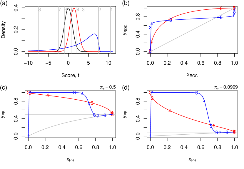
When comparing two ROC curves (from two ranking algorithms), the ideal scenario is that one curve dominates the other. More specifically, for each fixed value of , , i.e., the from curve A is at least as large as the from curve B. Alternatively, dominance could be described as for each fixed value of . In this case, ranking algorithm A is uniformly better than ranking algorithm B. In practice, however, we more often observe ROC curves that cross. Consider the two ROC curves shown in Figure 3(b) (full explanation to follow in Section 2). Ranking algorithm A is better if we consider values above 0.2 tolerable, while ranking algorithm B is better if we need less than 0.2. So we are faced with the question of which algorithm is best, subject to a maximum tolerable value for . This translates into how to choose the threshold.
A natural way to provide greater focus to small values of is afforded by the increasingly popular precision-recall (PR) curve (Raghavan et al., 1989; Provost et al., 1998; Davis and Goadrich, 2006; Brodersen et al., 2010). While the PR curve is used quite often in machine learning and information retrieval, it has received relatively little attention regarding its statistical inferential properties; the most notable exceptions are Davis and Goadrich (2006), Clémençon and Vayatis (2009), and Boyd et al. (2012). The PR curve parallels the ROC curve in many ways, but can actually be more informative in that it is affected by what is commonly called the prior probabilities. Prior probabilities represent class membership, and , and are rarely known in practice, but something can usually be said about the so-called skew defined as . ROC curves provide no information about skew and in fact are invariant to skew (Pepe, 2003; Fawcett, 2006; Krzanowski and Hand, 2009). On the other hand, PR curves are very much a function of the class probabilities and tend to be more useful in cases of imbalance (i.e., skew not equal to one); see Raghavan et al. (1989); Davis and Goadrich (2006); Clémençon and Vayatis (2009); Boyd et al. (2012).
For example, consider the extremely desirable ROC point when . If the goal is to rank-order instances to find members of the class (e.g., predicting emails as scam), one will be interested in the probability that an instance is given it was predicted as . This probability is a minuscule .09, thus suggesting the desirable ROC point is actually a complete failure. The PR curve places this ROC point when in an undesirable region because it becomes the PR point , where optimality is far away at . Using exactly the same input as the ROC curve, the PR curve provides a summary regarding utility of an algorithm for finding members of the class, making the PR curve a very viable tool. Proper use of the PR curve (and any summaries obtained from it) should be guided by the properties and limitations of this curve.
The remainder of this paper is organized as follows. Section 2 defines and presents properties of the PR curve when complete distributional assumptions are specified for scores from both classes. Complete proofs are given for properties of these population PR curves. Six sets of distributional assumptions serve to illustrate the various properties, including bi-normal, bi-beta, overlapping uniforms, subset ranges for continuously-defined scores, and overlapping ranges for discretely defined scores. Section 3 defines and present properties of a nonparametric (empirical) estimator of the PR curve; small-sample and asymptotic behavior are studied. Concluding remarks are given in Section 4.
2 Defining PR Curves from Population Scores
In this section, we first define population PR curves as arising when full distributional information is known, then investigate some relevant properties. Finally, full details of these population PR curves and their properties are illustrated using six cases that include discrete and continuous scores.
2.1 Definitions
Ranking algorithms produce a score, , that is used in predicting class membership for an instance (also commonly referred to as an item, record, object, etc.). Without loss of generality, assume large values of are consistent with membership in class and small values of are consistent with membership in class . is viewed as a random variable whose distribution depends on the true (unknown) class. For a specified threshold , one can consider the joint distribution of true and predicted class membership as given in Table 1. This population-level confusion matrix can change with changing values of threshold , but for a given it can be summarized using only three numbers. In fact, provided and , the confusion matrix can be uniquely and equivalently represented using either triplet
| (1) |
or triplet
| (2) |
| Truth | ||||
| Predicted | ||||
The ROC curve is based on representation (1) and plots as a function of . For all values of , the ROC curve plots , where
and and are the distribution functions of score for different classes. To more directly identify as a function of rather than as a function of , we can write , where is the generalized inverse of distribution function . Hence, the ROC curve is
| (3) |
It is interesting to note that although motivated by triplet representation (1) of the population-level confusion matrix in Table 1, the ROC curve actually ignores class probability that is a part of the triplet. This is often described as an advantage of the ROC curve (Pepe, 2003; Fawcett, 2006; Krzanowski and Hand, 2009). But, depending on the intended usage of ranking results, this could be a disadvantage, as demonstrated in the introduction.
The PR curve is based on representation (2) and plots as a function of for all values of . The precision, , is the probability that an instance is given it was predicted . In medical testing, precision is usually referred to as the positive predictive value. Originating in the specialty of information retrieval, the term recall is equivalent to , hence the name of the PR curve. For all values of , the PR curve plots , where
| (4) |
and hence
| (5) |
2.2 Properties
We now consider some useful properties of PR curves, with proofs given in the Appendix. Some, but not all, of these properties have been presented or even proved elsewhere, while for others we provide refined statements. Boyd et al. (2013a, b) suggest that the PR curve decreases to as recall increases to one; while this is often the case, we demonstrate that this is not guaranteed. Clémençon and Vayatis (2009) correctly argue that the PR curve approaches as recall increases to one when and have the same support; we derive the limit even when and have differing support. In fact, Clémençon and Vayatis (2009) limit all discussion to continuous and having the same support, but this paper takes a broader view on the set of possible and that might occur in practice. Although conditions for monotonicity of the PR curve have been addressed by Clémençon and Vayatis (2009) and lower bounds on the PR curve have been addressed by Boyd et al. (2012), this paper adds to those contributions.
As above, the ranking-algorithm score is assumed to be a random variable with distribution functions and in the and classes. For each of and , the possible values of the score range from to . If scores are continuous random variables, they have densities and .
Quantile functions or generalized inverse distribution functions are heavily used below. The usual definition is used, that is, for , where it is understood that . Many properties result (see Embrechts and Hofert, 2013), including: is nondecreasing; if , is left-continuous at and admits a limit from the right at ; and ; and and if is strictly increasing. These properties allow us to conclude that and , but .
Proofs for the following properties are provided in Appendix A:
-
P1.
The ROC curve is nondecreasing, with (one-sided) limiting values as follows:
-
(a)
.
-
(b)
.
-
(a)
-
P2.
The PR curve is not necessarily monotone, with (one-sided) limiting values as follows:
-
(a)
.
-
(b)
If the maximum possible score among members of class is at least as large as the maximum possible score among members of class (i.e., ), then , where may be infinity.
-
(c)
If , then .
-
(a)
-
P3.
Monotonicity of the PR curve.
-
(a)
If the ROC curve is concave and , then the PR curve is nonincreasing.
-
(b)
If the ROC curve is convex, , and , then the PR curve is nondecreasing.
-
(a)
-
P4.
Chance Curves. A ranking algorithm is useless if score distributions are the same across classes. If the populations of scores for and are identical, then chance ROC and PR curves are
with equality at values of and for which and for a unique .
-
P5.
Perfect-Separation Curves. The ideal ROC and PR curves occur when all scores for the class exceed all scores for the class, meaning . The perfect-separation ROC and PR curves are actually not true functions because each curve can have multiple ordinates for the same abscissa. For this reason, it is more convenient to describe these perfect-separation curves as a function of threshold, as follows and graphed in Figure 1:
and

Figure 1: Perfect-separation ROC and PR curves. -
P6.
Reverse-Separation Curves. In the event that all scores for the class are exceeded by all scores for the class (i.e., ), one could simply multiply all scores by negative one to yield perfect-separation ROC and PR curves. Nonetheless, it is interesting to investigate the scenario when because it represents the lower bounds on these curves. The reverse-separation ROC and PR curves are actually not true functions because each curve can have multiple ordinates for the same abscissa. For this reason, it is more convenient to describe these reverse-separation curves as a function of threshold, as follows and graphed in Figure 2:
and
Moreover, the achievable lower bound curves are
and

Figure 2: Reverse-separation ROC and PR curves. -
P7.
Invariance to increasing transformation. ROC and PR curves are unaffected if the same increasing transformation is applied to scores for both classes.
2.3 Illustrations
Properties P1–P7 are illustrated using six cases described below and depicted in Figures 3–6. Cases C and D are motivated by Boyd et al. (2013a). Cases A and B are depicted in Figure 3, Case C is depicted in Figure 4, Cases D and E are depicted in Figure 5, and Case F is depicted in Figure 6. Each case may be viewed as output from a ranking algorithm, meaning scores are assigned to instances in the and classes. An effective ranking algorithm tends to produce highly separated scores for the classes.
- Case A:
-
Scores follow the popular bi-normal model, meaning scores from the class are distributed as normal with mean and variance , while scores from the class are distributed as normal with mean and variance . For consistency with large scores suggesting the class, . For depiction in Figure 3, values are set as , and . Because and , the ROC curve starts at (0,0), is nondecreasing, and ends at (1,1), according to P1. The ROC curve is concave because increases with (see proof of P3). Given that the ROC curve is concave and , P3 says the PR curve is nonincreasing, and by P2 the PR curve starts at (0,1) and ends at . PR curves are shown for and , to demonstrate the impact of imbalance; the class is ten times as likely as the class when .
This ranking algorithm performs better than random (exceeds the chance curve) for both ROC and PR curves over all thresholds. The PR curve is much closer to the perfect-separation curve when than when .
- Case A*:
-
Scores follow a bi-lognormal model, meaning scores from the class are distributed as lognormal with parameters and , while scores from the class are distributed as lognormal with parameters and . Because the same log transformation can be applied to scores from both the and classes to simultaneously convert the bi-lognormal model to a bi-normal model, property P7 tells us the ROC and PR curves will match those displayed in Figure 3 for the bi-normal model.
- Case B:
-
Scores from the class are distributed as normal with mean and variance . Scores from the class are distributed as , where follows a lognormal distribution with parameters and . Letting and denote the standard normal distribution and inverse distribution functions, the class-level distribution functions are and , with , , and . By P1, the ROC curve starts at (0,0), is nondecreasing, and ends at (1,1). But the ROC curve is neither concave nor convex because is not a monotone function of . The PR curve is non-monotone, starting at (0,0) (by P2), increasing, then decreasing, then increasing again to end at (by P2).
This ranking algorithm is near-perfect for large thresholds (i.e., , which results in , and as large as 0.7, and when ), but is worse than random for very small thresholds (i.e., ). One could argue, however, that the region where it performs poorly () is of limited practical relevance because one would rarely consider using a threshold that results in a 75% false-positive rate. Comparing performance of ranking algorithms from Cases A and B, ranking algorithm B is clearly better in regions of practical relevance, especially considering the PR curve when . The choice of thresholds is clearly a critical component to comparing and choosing among ranking algorithms.
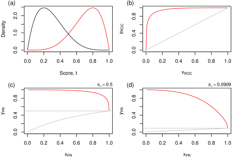
Figure 4: Densities, ROC curve, and PR curves for Case C. (a) Density functions for: the beta(2,5) distribution as the black curve, corresponding to the class; and for the beta(5,2) distribution as the red curve, corresponding to the class. (b) ROC curve, where the gray diagonal line is the chance curve. (c) PR curve assuming balanced classes so that . The gray horizontal line is the chance curve, while the other gray curve is the achievable lower bound curve. (d) Same as (c), except assuming the class is ten times as likely as the class so that . - Case C:
-
Scores follow a bi-beta model with scores for the class distributed as beta with parameters 2 and 5, and the class distributed as beta with parameters 5 and 2. Both ROC and PR curves are well behaved. The ROC curve starts at (0,0), increases to (1,1), and is concave because increases with , where and . As a result, the PR curve is decreasing from its starting point of (0,1) (by P3) to end at (by P2). The bi-beta model is particularly well-suited to scenarios where scores are bounded, and the beta distribution offers a variety of shapes (e.g., levels of skewness).
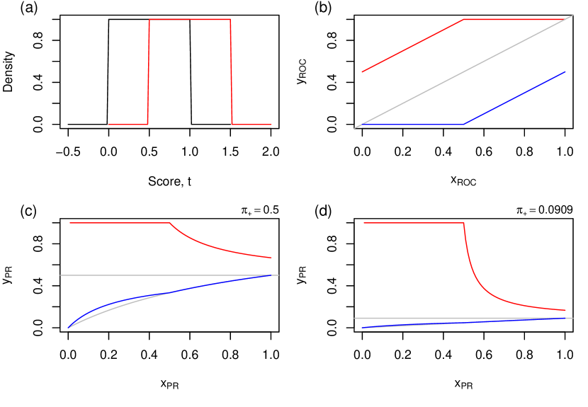
Figure 5: Densities, ROC curves, and PR curves for Cases D and E. (a) Density functions for the uniform [0,1] distribution as the black curve and the uniform [0.5,1.5] as the red curve; vertical reference lines delineate the possible values for each density. For case D, the black curve corresponds to the class and the red curve to the class. Case E is the reverse of Case D. (b) ROC curves: Case D is the red curve, Case E is the blue curve. The gray diagonal line is the chance curve. (c) PR curves assuming balanced classes so that : Case D is the red curve, Case E is the blue curve. The gray horizontal line is the chance curve, while the other gray curve is the achievable lower bound curve. (d) Same as (c), except assuming the class is ten times as likely as the class so that . - Case D:
-
Scores have non-subset ranges, with scores for the class distributed as uniform on and scores for the class distributed as uniform on . By P1, the ROC curves starts at , which might at first seem strange but is a consequence of the overlapping but non-subset relationship between the possible scores for different classes. More specifically, the ROC curve does not start at (0,0) because . Also by P1, the ROC curve is nondecreasing and ends at (1,1). The ROC curve is concave because for , 1 for , for is nondecreasing in . Consequently, the PR curve is nonincreasing by P3 and by P2 it starts at (0,1) and ends at . The PR curve does not end at as with the previous cases because , resulting in . The endpoint is (1,2/3) for balanced classes, and (1,1/6) when the class is ten times more likely than the class.
- Case E:
-
This is Case D, except the scores are reversed for the classes. That is, scores for the class are distributed as uniform on , and scores for the class are distributed as uniform on [0,1]. Operationally, large scores should suggest the class, so this ranking algorithm is expected to perform rather poorly. The ROC curve is still nondecreasing, but it is now below the chance curve, indicating a completely ineffective ranking algorithm (which is as expected). The ROC curve starts at (0,0) and ends at (1,0.5) by P1; it does not end at (1,1) because . The ROC curve is convex because for , 1 for , 0 for is nonincreasing in . By P3, the PR curve is nondecreasing because the ROC curve is convex, , and . By P2, the PR curve starts at (0,0) and ends at (1,).
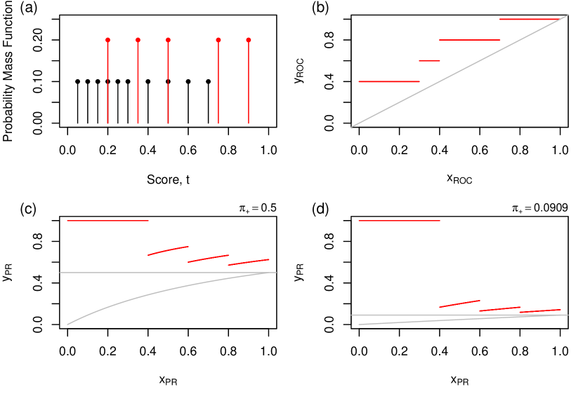
Figure 6: Probability mass functions, ROC curve, and PR curves for Case F. (a) Probability mass functions: the discrete uniform on 0.05, 0.1,.15, 0.2, 0.25, 0.3, 0.4, 0.5, 0.6, 0.7 as the black dots, corresponding to the class; and discrete uniform on 0.2, 0.35, 0.5, 0.75, 0.9 as the red dots, corresponding to the class. (b) ROC curve, where the gray diagonal line is the chance curve. (c) PR curve assuming balanced classes so that . The gray horizontal line is the chance curve, while the other gray curve is the achievable lower bound curve. (d) Same as (c), except assuming the class is ten times as likely as the class so that . - Case F:
-
This case demonstrates ranking-algorithm scores where only a finite number of possible values are allowed, i.e., the scores are discrete random variables. Scores for the class follow a discrete uniform distribution with 10 possible score values of 0.05, 0.1, 0.15, 0.2, 0.25, 0.3, 0.4, 0.5, 0.6, and 0.7. Scores for the class follow a discrete uniform distribution with five possible score values of 0.2, 0.35, 0.5, 0.75, and 0.9. Because and , P1 implies the ROC curve is nondecreasing, starting at and ending at . Nothing can be said about monotonicity of the PR curve because the ROC curve is neither concave or convex. In fact, it can be seen that the PR curve is not monotone; it consists of continuous nondecreasing pieces separated by jumps. By P2, the PR curve starts at (0,1) and ends at . The PR curve endpoint is (1,0.625) for balanced classes, and (1,0.143) when the class is ten times more likely than the class.
This case provides a preliminary view of what to expect from empirical estimation of the PR curve. Observed scores, even from continuous distributions, will be countable sets that may be viewed as arising from discrete distributions. Section 3.1 further addresses this connection.
3 Empirical PR Curves
In this section, we define empirical PR curves as obtained from observed scores without additional distributional assumptions. Stochastic convergence properties are presented and investigated using small-sample simulation studies.
3.1 Definitions and Asymptotics
Suppose we observe independent random samples of scores from the class and from the class, where is the total number of items or instances. Let and denote the class-level empirical distribution functions, i.e., and , where is the indicator function. Ignoring class membership and combining all scores as , also define .
A popular and computationally efficient empirical estimator of the PR curve results from estimating the pair (recall , precision) for different thresholds as described in (4). A natural selection of threshold values is the set of distinct scores observed (collectively over both classes). In other words, an estimated PR curve is
To avoid division by zero while not using if-then-else statements, sometimes the slightly modified definition
is used. Neither nor present as functional definitions for estimated precision as a function of recall. More importantly, they can result in multiple distinct values of estimated precision for a single value of recall. This creates confusion when evaluating metrics such as area under the PR curve. Davis and Goadrich (2006) and Boyd et al. (2013a) extensively investigate this issue. They also give guidance on the proper interpolation that should be used to fill in the gaps created in the estimated PR curve based on estimators and . Clearly, a functional definition would avoid the need for interpolation.
This author sides with Clémençon and Vayatis (2009) in recommending the estimator that naturally comes from the functionally defined PR curve as presented in (5), but applied using and in place of and . Specifically, consider the empirical estimator of the PR curve
This estimator is free of the disadvantages given above for and . While it requires computation of the inverse empirical distribution function , also known as the empirical quantile function, the additional computations are well worth the benefits.
Some properties of are clearly demonstrated in Figure 6 showing Case F based on discrete distributions for scores. Sampling, even from continuous score populations, will result in empirical distribution functions that are step functions as in Case F. The resulting curve consists of at most disjoint segments, each associated with distinct values of observed . Suppose the points of discontinuity occur at . Then the segments are defined on , and . is either continuous or continuous from the right at . Estimated precision is an increasing function on each segment. Furthermore, at points of discontinuity, the limit from the left of the estimated precision curve is larger than the limit from the right, i.e., .
An extensive body of literature focuses on asymptotic properties of the empirical ROC curve ; see, for example, Csörgő (1983), Hsieh and Turnbull (1996), Pepe (2003), and Bertail et al. (2009). Building on this body of literature to take advantage of the similarity between the empirical ROC and as appearing in , then applying a multivariate Taylor approximation to the function that converts to obtain , Clémençon and Vayatis (2009) obtain the following strong approximation result for .
Theorem 1 (Strong approximation)
Suppose and have densities and , and the following conditions hold:
-
1.
For some , the slope of the function is bounded on , i.e.,
(6) -
2.
The density
-
(a)
is differentiable,
-
(b)
does not vanish for , i.e.,
-
(c)
and has controlled tail behavior in that there exists such that
(7)
-
(a)
Then, we almost surely have, as :
-
A.
The empirical PR curve is strongly consistent, uniformly over , i.e.,
-
B.
There exist two independent sequences of Brownian bridges and
, and a Gaussian random variable independent from the Brownian bridges, such that uniformly over :
Moreover, pointwise limits are obtained for a fixed in as
where
and and .
Note that a typo has been corrected in (B.), namely replaced a in the first term of . Typos have also been corrected in (1): the last two terms of were missing multipliers , and inverse distribution functions were needed in two places. For defining tail behavior, has been included in (7), in the spirit of Parzen (1979).
The variance decomposition presented in (1) has interesting properties. Variance clearly increases as (i.e., imbalance) increases. The slope of the function as given in (6) is important, with variance being a quadratic function of this slope; variance can quickly increase for large slopes. On the other hand, the slope being zero causes the second term of the variance to vanish. The first and third term of the variance vanish when ; this happens when scores have different ranges across classes, with the class having larger values. The third term of the variance also vanishes when ; this happens when scores have different ranges across classes, with the class having smaller values.
The normal approximations suggested by (B.) work very well for some situations, even for relatively small and large . On the other hand, they are completely inappropriate in other situations. These comments are further discussed in the following subsection.
3.2 Small-sample Properties
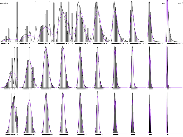
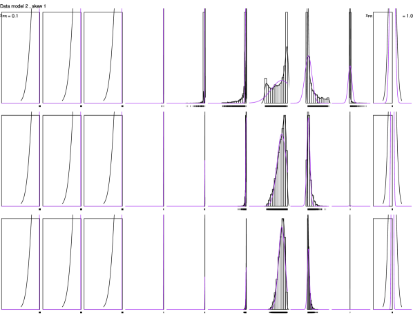
To study the small-sample behavior of , samples of sizes using (corresponding to ) were generated from Cases A, B, C, D, and F. Some of the resulting histograms, based on 5000 simulation replicates, of are shown in Figures 7–11, at . For a particular data-generating mechanism and a value for , these figures show histograms of , , …, for . A kernel density estimate is shown along with each histogram, and in some figures approximating normal densities as obtained from (1) are also shown. In situations where the normal approximation is valid, we expect the kernel density to coincide with the normal density, with improved performance for increasing , where the top row of histograms correspond to and the bottom row to .
Consider Case A where scores have the same range for both classes (meaning and have equal support), and class-specific densities have exponential-type tail behavior with in (7). The slope in (6) gets very large as approaches 1, but is less than 5 when . These are near-ideal conditions for the normal approximation to hold. Figure 7 demonstrates that even with a large and relatively small , resulting in a small on average, the normal approximation from (1) very nearly matches the kernel density when . The normal approximation does not perform well near the extremes, namely close to zero or one; this is no surprise as the approximation in (B.) is valid for for .
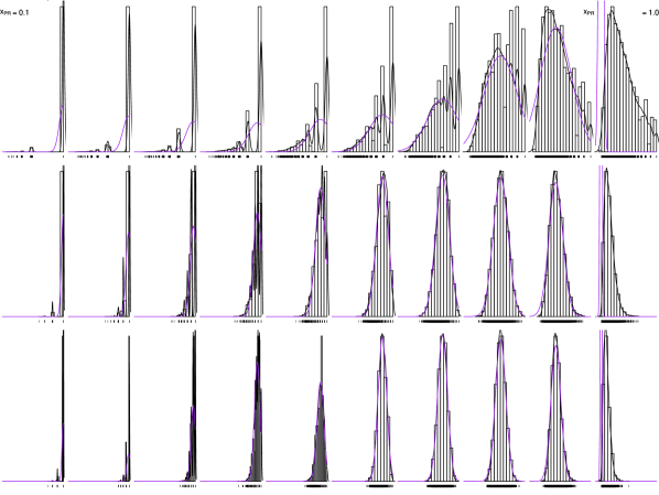
For other situations, much larger is needed to deal with the same value of . Consider Case C where scores again have the same range for both classes. A major difference from Case A is that the scores of Case C have finite range, corresponding to which by itself would yield faster convergence. However, the slope from (6) can be very large, especially for . This will serve to destabilize the second term of in (B.). The second term of in (B.) also suggests that decreasing the may offset the effect of large slope. In fact, all three terms in are expected to become more stable as approaches one. Additionally, when , essentially dropping the first and third terms from . All of this results in slower convergence, as demonstrated in Figure 8.
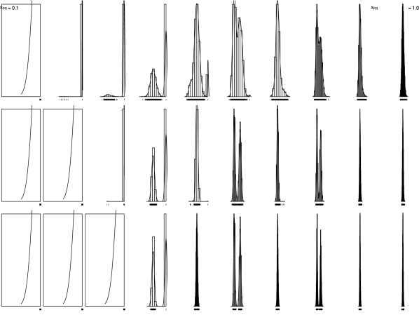
The shortcomings and limitations of Theorem 1 are quite enlightening. First, the results do not apply to scores observed from discrete populations. This, of course, is obvious because the theorem calls for densities that do not exist. However, other limitations exist. Figure 9 corresponding to Case F demonstrates that may be inconsistent. For the “best” scenario of and , the distributions of , , and are all bimodal. As may be seen in Figure 6, is discontinuous at exactly the same values of . The root cause of inconsistency is that is only consistent for provided is continous at (Csörgő, 1983, p.5). Scores from discrete distributions violate this condition.
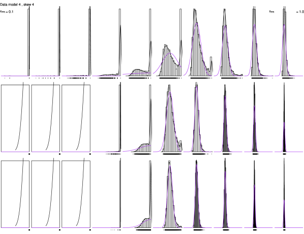
Theorem 1 may be thoughtfully applied even when scores do not have the same range for both classes. Consider Case D. When , then and consequently, and . Hence, (B.) yields , so the limiting distribution is degenerate. Moreover, the difficulty of estimating the boundary where the class densities no longer overlap has the consequence that larger and smaller will be needed for the normal approximation to be reasonable even when . See Figure 10 for Case D with . Even when , the approximation is reasonable only for .
The very poor performance of the normal approximation in Case B may be somewhat surprising. See Figure 11 for Case B when ; the approximation is far worse for other values of skew. The tail behavior of the lognormal distribution yields , resulting in the slowest convergence rate among all cases considered in this article. When , both and are essentially zero, causing all three terms in to practically drop out. When , is again neglible, causing the second term in to practically drop out. Also when , is so close to one that the Brownian bridge is essentially degenerate, with practical consequence that basically has only the first term.
4 Concluding Remarks
This paper contains a comprehensive exposition on properties of population PR curves. Some results have been previously presented, most notably by Davis and Goadrich (2006), Clémençon and Vayatis (2009), and by Boyd et al. (2012). Other results are new or conditions have been relaxed. By looking at a variety of distributional settings, defined according to Cases A to F, new results have been discovered.
This paper also investigates properties of the functional empirical estimator of the PR curve. It is quite alarming that is not consistent at points corresponding to positive probability from discrete distributions of scores in the class. For continuously-defined scores, strong approximation is useful but convergence rates can be heavily influenced by the distributional setting, the , and the point of interest on the PR curve.
While the population and empirical PR curves inherit many properties from their ROC counterparts, PR curves have several complexities not seen in ROC curves. A thorough understanding of these complexities will allow users to avoid misuse or misinterpretation.
Appendix A
Properties of ROC and PR curves as given in Section 2.2 are proved below.
-
P1.
Proof By equation (3), for . As stated above, distribution functions and their generalized inverses are nondecreasing functions. Hence, is nonincreasing in , so that is also nonincreasing in , and finally is nondecreasing in for .
Noting that and , we get . Similarly, .
-
P2.
Proof To show possible non-monotonicity, consider continuous ranking-algorithm scores that admit densities. From equation (5),
(10) where . Monotonicity of the PR curve is determined by monotonicity of for a fixed value of . Because
(11) can be positive or negative, the PR curve can decrease or increase as changes for a fixed . Moreover,
yields (a). When ,
because , and this yields (c). Because when , using l’Hopital’s Rule we get
to yield (b).
-
P3.
Proof Concavity or convexity of the ROC curve implies continuity of the distribution functions, and hence existence of densities. From equation (3),
and define . If the ROC curve is concave (meaning is nondecreasing as decreases), then is nondecreasing as increases, i.e., . Similarly, if the ROC curve is convex. Now consider the PR curve as defined in (10) and whose monotonicity is determined by the monotonicity of . By (11), the sign of equals the sign of
Moreover,
It is helpful the clarify the role of thereshold . The earlier view of allowed us to characterize the shape of function for changing values of threshold : either or for all , based on concavity or convexity of the ROC curve. For studying monotonicity of the PR curve, however, the threshold must be viewed as as used in the expression for above.
-
(a)
If the ROC curve is concave, then implies , so is nonincreasing as increases. As a result,
But implies , so
Consequently, , and so the PR curve is nonincreasing.
-
(b)
If the ROC curve is convex, then implies , so is nondecreasing as increases. As a result,
But implies , and , so . Consequently, , and so the PR curve is nondecreasing.
-
(a)
-
P4.
Proof For the ROC curve, applied to (3) yields
by property of generalized inverse distribution functions, with equality when is strictly increasing.
-
P5.
Proof Let us first consider for different values of threshold . For , because , hence . For the same reason, for , so . For other allowable thresholds, , and increases to one as decreases.
Now consider . For , and increases to one as decreases. Because for , for . This completes the perfect-separation ROC curve. Note that property P1 regards , thus ignoring the other possible values of that correspond to , and that the resulting becomes a legitimate function.
Given the perfect-separation ROC curve, use (4) to get
and
which yields the result. Note that property P2 regards , thus ignoring the other possible values of that correspond to , and that the resulting becomes a legitimate function.
-
P6.
Proof First consider . For , and increases to one as decreases. For , and so .
Now consider . For , because . For , and increases to one as decreases. This completes the reverse-separation ROC curve.
Given the reverse-separation ROC curve,
and use a slight modification of (4) to get
which yields the reverse-separation PR curve.
Because is a probability, is clearly bounded below by zero, and this lower bound is achieved by the reverse-separation ROC curve.
As a probability, precision (i.e., ) is clearly bounded below by zero, but there is a much tighter bound. By properties of distribution functions, , so
Hence, with a slight modification to (5),
Furthermore, this lower bound is achieved by the reverse-separation PR curve as demonstrated above.
-
P7.
Proof First consider an ROC curve based on the original score :
Now consider an increasing function with inverse . Then the ROC curve based on the transformed score , using thresholds such that , is
Hence, the transformed scores lead to the same ROC curve as the original scores.
Similarly,
Hence, the transformed scores lead to the same PR curve as the original scores.
References
- Bertail et al. (2009) Patrice Bertail, Stéphan J. Clémençcon, and Nicolas Vayatis. On bootstrapping the ROC curve. In Proceedings of Neural Information Processing Systems 21 - NIPS ’08, pages 137–144, Vancouver, Canada, 2009. Curran Associates, Inc. URL http://papers.nips.cc/paper/3404-on-bootstrapping-the-roc-curve.pdf.
- Boyd et al. (2012) Kendrick Boyd, Vítor Santos Costa, Jesse Davis, and C. David Page. Unachievable region in precision-recall space and its effect on empirical evaluation. In Proceedings of the 29th International Conference on Machine Learning, ICML’12, pages 1619–1626, USA, 2012. Omnipress. ISBN 978-1-4503-1285-1. URL http://dl.acm.org/citation.cfm?id=3042573.3042780.
- Boyd et al. (2013a) Kendrick Boyd, Kevin H. Eng, and C. David Page. Area under the precision-recall curve: Point estimates and confidence intervals. In H. Blockeel, K. Kersting, S. Nijssen, and F. Železný, editors, Machine Learning and Knowledge Discovery in Databases - European Conference, ECML PKDD 2013, Prague, Czech Republic, September 23-27, 2013, Proceedings, Part III, pages 451–466. Springer, Berlin, Heidelberg, 2013a. ISBN 978-3-642-40993-6. doi: 10.1007/978-3-642-40994-3˙29. URL https://doi.org/10.1007/978-3-642-40994-3_29.
- Boyd et al. (2013b) Kendrick Boyd, Kevin H. Eng, and C. David Page. Erratum: Area under the precision-recall curve: Point estimates and confidence intervals. In Machine Learning and Knowledge Discovery in Databases - European Conference, ECML PKDD 2013, Prague, Czech Republic, September 23-27, 2013, Proceedings, Part III. Springer, Berlin, Heidelberg, 2013b. doi: 10.1007/978-3-642-40994-3˙55. URL https://doi.org/10.1007/978-3-642-40994-3_55.
- Brodersen et al. (2010) Kay Henning Brodersen, Cheng Soon Ong, Klaas Enno Stephan, and Joachim M. Buhmann. The binormal assumption on precision-recall curves. In 2010 20th International Conference on Pattern Recognition, pages 4263–4266. IEEE, 2010. doi: 10.1109/icpr.2010.1036.
- Clémençon and Vayatis (2009) Stéphan Clémençon and Nicolas Vayatis. Nonparametric estimation of the precision-recall curve. In Proceedings of the 26th International Conference on Machine Learning - ICML ’09, pages 185–192, New York, NY, USA, 2009. ACM Press. ISBN 978-1-60558-516-1. doi: 10.1145/1553374.1553398. URL http://doi.acm.org/10.1145/1553374.1553398.
- Csörgő (1983) Miklós Csörgő. Quantile Processes with Statistical Applications. SIAM, Philadelphia, 1983. ISBN 9780898711851.
- Davis and Goadrich (2006) Jesse Davis and Mark Goadrich. The relationship between precision-recall and ROC curves. In Proceedings of the 23rd International Conference on Machine learning - ICML ’06, pages 233–240, New York, NY, USA, 2006. ACM Press. ISBN 1-59593-383-2. doi: 10.1145/1143844.1143874. URL http://doi.acm.org/10.1145/1143844.1143874.
- Embrechts and Hofert (2013) Paul Embrechts and Marius Hofert. A note on generalized inverses. Mathematical Methods of Operations Research, 77(3):423–432, 2013. URL https://EconPapers.repec.org/RePEc:spr:mathme:v:77:y:2013:i:3:p:423-432.
- Fawcett (2006) Tom Fawcett. An introduction to ROC analysis. Pattern Recognition Letters, 27(8):861–874, 2006. doi: 10.1016/j.patrec.2005.10.010.
- Hsieh and Turnbull (1996) Fushing Hsieh and Bruce W. Turnbull. Nonparametric and semiparametric estimation of the receiver operating characteristic curve. Annals of Statistics, 24(1):25–40, 1996. doi: 10.1007/s10822-014-9808-1.
- Krzanowski and Hand (2009) Wojtek J. Krzanowski and David J. Hand. ROC Curves for Continuous Data. Chapman and Hall/CRC Press, 2009. ISBN 9781439800225.
- Parzen (1979) Emanuel Parzen. Nonparametric statistical data modeling. Journal of the American Statistical Association, 74(365):105–121, 1979. doi: 10.1080/01621459.1979.10481621. URL https://amstat.tandfonline.com/doi/abs/10.1080/01621459.1979.10481621.
- Pepe (2003) Margaret S. Pepe. The Statistical Evaluation of Medical Tests for Classification and Prediction. Oxford University Press, New York, 2003. ISBN 0198509847.
- Provost et al. (1998) Foster J. Provost, Tom Fawcett, and Ron Kohavi. The case against accuracy estimation for comparing induction algorithms. In Proceedings of the Fifteenth International Conference on Machine Learning, ICML ’98, pages 445–453, San Francisco, CA, USA, 1998. Morgan Kaufmann Publishers Inc. ISBN 1-55860-556-8. URL http://dl.acm.org/citation.cfm?id=645527.657469.
- Raghavan et al. (1989) Vijay Raghavan, Peter Bollmann, and Gwang S. Jung. A critical investigation of recall and precision as measures of retrieval system performance. ACM Transactions on Information Systems, 7(3):205–229, 1989. ISSN 1046-8188. doi: 10.1145/65943.65945. URL http://doi.acm.org/10.1145/65943.65945.