Reverse Quantum Annealing Approach
to Portfolio Optimization Problems

Abstract

We investigate a hybrid quantum-classical solution method to the mean-variance portfolio optimization problems. Starting from real financial data statistics and following the principles of the Modern Portfolio Theory, we generate parametrized samples of portfolio optimization problems that can be related to quadratic binary optimization forms programmable in the analog D-Wave Quantum Annealer 2000Q^TM. The instances are also solvable by an industry-established Genetic Algorithm approach, which we use as a classical benchmark. We investigate several options to run the quantum computation optimally, ultimately discovering that the best results in terms of expected time-to-solution as a function of number of variables for the hardest instances set are obtained by seeding the quantum annealer with a solution candidate found by a greedy local search and then performing a reverse annealing protocol. The optimized reverse annealing protocol is found to be more than 100 times faster than the corresponding forward quantum annealing on average.

Keywords:	Portfolio Optimization, Quadratic Unconstrained Binary
	Optimization, Quantum Annealing, Genetic Algorithm,
	Reverse Quantum Annealing
JEL classification:	C61, C63, G11

1 Introduction

One reason behind the current massive investment in quantum computing is that this computational paradigm has access to resources and techniques that are able to circumvent several bottlenecks of state-of-the-art digital algorithms. Much research is today devoted to understanding how to exploit this power to deliver high quality solutions to discrete optimization problems at a fraction of the time required using the best classical methods on high-end hardware.

Quantum annealers are special-purpose machines inspired by the adiabatic quantum computing paradigm. These machines are manufactured by D-Wave Systems and appeared on the market in 2011, and while being limited in programmability with respect to other experimental devices under testing by other companies, are still the only available quantum devices that feature a sufficient amount of quantum memory (qubits) to be applied to non-trivial problems at the time of writing. For this reason they are subject to extensive empirical investigation by several groups around the world, not only for scientific and research purposes [1, 2], but also for performance evaluation on structured real world optimization challenges [3, 4, 5]. It is expected that as quantum computing devices mature, they’d become available to enterprises for use through dedicated cloud services [6].

Optimization problems comprise a large class of hard to solve financial problems, not to mention the fact that many supervised and reinforcement learning tools used in finance are trained via solving optimization problems (minimization of a cost function, maximization of reward). Several proposed applications of the D-Wave machine to portfolio optimization [7, 8], dealt with portfolios that were too small to evaluate the scaling of the chosen approach with the problem size. In this paper we go beyond these early approaches and provide an analysis on sufficient data points to infer a scaling and measure a limited speedup with respect a state-of-the-art numerical method based on genetic algorithms. Moreover, we extensively tune the D-Wave machine’s runs using the hybrid method of Reverse Annealing which is available only on the most advanced models to date, and whose usage has never been published before on structured optimization problems.

Portfolio optimization

The optimal portfolio construction problem is one of the most extensively studied problems in quantitative finance. The Modern Portfolio Theory (MPT) as formulated by Markowitz [9] has laid the foundation for highly influential mean-variance portfolio optimisation approach. According to the MPT, a typical portfolio optimisation problem can be formulated as follows. Let $N$ be the number of assets, $\mu_{i}$ be the expected return of asset $i$, $\sigma_{ij}$ be the covariance between the returns for assets $i$ and $j$, and $R$ be the target portfolio return. Then the decision variables are the weights $w_{i}$, i.e. the investment associated with asset $i$ ($w_{i}\in\mathbb{R}$). The standard Markowitz mean-variance approach consists in the constrained, quadratic optimisation problem:

$$\min\sum_{i=1}^{N}\sum_{j=1}^{N}w_{i}w_{j}\sigma_{ij}\;\;; \sum_{i=1}^{N}w_{i}=1\;\;; \sum_{i=1}^{N}w_{i}\mu_{i}=R\;.$$ (1)

Quadratic problems of the form (1) are efficiently solvable by standard computational means (e.g., quadratic programming with linear constraints [10]) if the covariance matrix is positive definite. Interestingly, the problem can also be cast into an unconstrained quadratic optimization problem (QUBO) which is a suitable formulation for quantum annealers. This observation spurred in the last few years a couple of proof-of-principle papers that were performing runs on the first generation D-Wave machines solving discrete portfolio optimization problems [7, 8]. The discrete portfolio optimization problem is much harder to solve than continuous mean-variance portfolio optimization problem due to strong non-linearity, and is known to be NP-complete [11].

In this paper we propose an original approach to portfolio optimization that extends the mean-variance model to a general dependence structure and allows portfolio managers to express discretionary views on relative attractiveness of different assets and their combinations. The manuscript is structured as follows: in Section 2 the formulation of the portfolio optimization problem is constructively described starting from real market data. Section 3 describes the hybrid quantum annealing solver and its setup. Section 4 is devoted to the experimental results, including results obtained with the classical Genetic Algorithm (GA) benchmark (following [12]). In Section 5 we conclude with a discussion and considerations for future work.

2 Portfolio Optimization Beyond Markowitz

The problem we are trying to solve here is construction of the optimal portfolio from the assets with known characteristics such as asset returns, volatilities and pairwise correlations. A typical portfolio optimization problem consists of selecting $M$ assets from the universe of $N$ investible assets. These $M$ assets should ideally be the best possible choice according to some criteria. The scenario we target is a Fund of Funds portfolio manager who is facing a task of selecting the best funds that follow particular trading strategies (e.g., EM Macro Funds) in order to maximize the risk-adjusted returns according to some model.

A realistic case occurs when the assets are selected with equal preference weights (a classical example of exposure to equally weighted assets is the CSO portfolio). Should we want to generalize the portfolio with larger allocation to a given asset, we could allow for multiples of the reference weight by cloning an asset and treating it as a new one.

The task of encoding the relationship among the choices of $M$ funds (without replacement) from the universe of $N$ funds can then be formulated as a quadratic form:

$$O({\bf q})=\sum_{i=1}^{N}a_{i}q_{i}+\sum_{i=1}^{N}\sum_{j=i+1}^{N}b_{ij}q_{i}q_{j}\;,$$ (2)

where $q_{i}=1$ means that asset $i$ is selected and $q_{i}=0$ means that asset $i$ is not selected. Coefficients $a_{i}$ reflect asset attractiveness on a standalone basis and can be derived from the individual asset’s expected risk-adjusted returns. Coefficients $b_{ij}$ reflect pairwise diversification penalties (positive values) and rewards (negative values). These coefficients can be derived from the pairwise correlations.

The minimization of the QUBO objective function given by expression (2) should optimize the risk-adjusted returns by the use of the metrics of Sharpe ratio [13] for the $a_{i}$ parameters (measuring expected excess asset return in the asset volatility units) and correlation between assets (as a measure of diversification) for the $b_{ij}$ coefficients.

The Sharpe ratio is calculated as $(r-r_{0})/\sigma$ where $r$ is the asset’s expected annualized return, $r_{0}$ is the applicable risk-free interest rate and $\sigma$ is asset’s volatility (annualized standard deviation of the asset’s log-returns). The higher fund’s Sharpe ratio, the better fund’s returns have been relative to the risk it has taken on. Volatility can be estimated as historical annualized standard deviation of the Net Asset Value (NAV) per share log-returns. Expected return can be either estimated as historical return on fund investment or derived independently by the analyst/portfolio manager taking into account different considerations about the future fund performance. The asset correlation matrix $\rho_{ij}$ is constructed from the time series of log-returns [14].

QUBO instances

Instead of using the raw real numbers obtained from financial data for the QUBO coefficients, we opt to coarse-grain the individual funds Sharpe ratios and their mutual correlation values down to integer values by grouping intervals in buckets according to Table 1. By using bucketed values we define a scorecard, which is loosely based on the past fund performances but can be easily adjusted by portfolio manager according to his/her personal views and any new information not yet reflected in the funds reports. Indeed, in real world scenarios, optimization needs to be performed with respect to the discretionary views about the future held by portfolio manager, not necessarily with respect to automatically fetched market data. Moreover, if we assume that funds report their NAV per share on a monthly basis and we have comparable funds data for the previous year, then we only have 12 NAV observations in our time series from which we want to construct a correlation matrix for $N$ assets ($N\gg 12$). It is likely that the resulting correlation matrix will not be positive definite due to the number of observations being much smaller than the number of assets, ruling out the traditional solvers of mean-variance portfolio optimization problems which require a positive definite correlation matrix.

SR bucket (asset $i$)	Coefficient $a_{i}$
Equally spaced buckets,	Sample Mapping
from worst to best	Scheme
1st	15
2nd	12
3rd	9
4th	6
5th	3
6th	0
7th	$-$3
8th	$-$6
9th	$-$9
10th	$-$12
11th	$-$15

Correlation bucket	Coefficient $b_{ij}$
	Sample Mapping
	Scheme
$-1.00\leq\rho_{ij}<-0.25$	$-$5
$-0.25\leq\rho_{ij}<-0.15$	$-$3
$-0.15\leq\rho_{ij}<-0.05$	$-$1
$-0.05\leq\rho_{ij}<0.05$	0
$0.05\leq\rho_{ij}<0.15$	1
$0.15\leq\rho_{ij}<0.25$	3
$0.25\leq\rho_{ij}\leq 1.00$	5

Table 1: Specification of the sample QUBO coefficients from NAV time series market data

The instance set used for our case study is obtained by simulating asset values with the help of correlated Geometric Brownian Motion (GBM) processes with uniform constant asset correlation $\rho$, drift $\mu$ and log-normal asset volatility $\sigma$. The specific values of these parameters were derived from a wide range of fund industry researches (see, e.g., [15] for the Sharpe ratio distributions) and, therefore, can be viewed as representative for the industry. The simulation time horizon was chosen to be 1 year and the time step was set at 1 month $-$ this setup corresponds to the situation where a Fund of Funds portfolio manager is dealing with the short time series of comparable monthly fund performance reports. Detailed description of the simulation scheme can be found in Appendix A. Every simulated (or, ”realized”) portfolio scenario consists of 12 monthly returns for each asset. From these returns we calculated total realized return and realized volatility for each asset (which, obviously, differ from the their expected values $\mu$ and $\sigma$) and for the portfolio as a whole. We also calculated realized pairwise correlations between all assets according to the input uniform correlation $\rho$. Finally, we calculated individual assets and portfolio Sharpe ratios. For instance, with $\rho=0.1$, $\mu=0.075$, $\sigma=0.15$ and the constant risk-free interest rate set at $r_{0}=0.015$, the expected Sharpe ratio for each asset in a portfolio is 0.4. The expected Sharpe ratio for the portfolio of $N$ assets is significantly larger due to the diversification and low correlation between the assets, e.g., for a 48-asset portfolio we would expect Sharpe ratio values from 0.5 (25th percentile) to 2.1 (75th percentile) with a mean around 1.4.

Constraint on the number of selected assets

In QUBOs, the standard way to deal with the cardinality constraint (i.e., selection of only $M$ assets) would be to add a term $O_{\textrm{penalty}}({\bf q})$ to the objective function given by expression (2) such that the unsatisfying selections would be penalized by a large value $P\gg 1$, which would force the global minimum to be such that $\sum_{i=1}^{N}q_{i}=M$:

$$O_{\textrm{penalty}}({\bf q})=P\left(M-\sum_{i=1}^{N}q_{i}\right)^{2}\;.$$ (3)

Unfortunately, the introduction of such a large energy scale $P$ is typically associated with precision issues connected to the analog nature of the machine and the fact that there is a physical maximum to the energy that can be controllably programmed on local elements of the D-Wave chip [16]. However, several hybrid quantum-classical strategies can be put in place to overcome the limitation. For instance, we observe that shifting artificially the Sharpe ratio values by a constant amount $\pm\Delta$ (and adding buckets according to the prescription chosen, e.g., Table 1) will essentially amount to forcing the ground state solution of the unconstrained problem to have more or less desired number of assets selected. Hence, while not solving the same problem, we could imagine a solver of a similarly constrained problem that will enclose the quantum annealing runs in a classical loop which checks for the number of selected assets $m(\Delta)$ in the best found solution with $\Delta=0$, then increases or decreases the individual desirability of the assets according to whether $m$ is larger or smaller than $M$ and runs again until $m(\Delta)=M$ for $\Delta=\Delta^{\star}$. This sort of hybridization scheme is not uncommon for quantum-assisted solvers [17, 3] and the number of expected rounds of runs should scale as $\propto\log_{2}(\Delta^{\star})$ as per a binary search introducing a prefactor over the time-to-solution complexity which should stay manageable. Other hybrid approaches could also be put forward to deal with the constraint such as fixing some asset selections in pre-processing via sample persistence [18].

Per above arguments, in our benchmark case study in this work, we will focus on running unconstrained problems, setting $\Delta=0$. By design, the instance ensambles are such that the average number of assets in the ground state should be around $N/2$ (see Table 2) corresponding to the largest combinatorial space by exhaustive enumeration of the possible solutions, so our tests will arguably be targeting among the most challenging instances of our parametrized model.

3 Quantum Annealing Hybrid Solver

A QUBO problem can be easily translated into a corresponding Ising problem of $N$ variables $s_{i}$, $i=1,\ldots,N$ with $s_{i}\in\{+1,-1\}$ given by the following expression:

$$O_{\textrm{Ising}}({\bf s})=\sum_{i=1}^{N}h_{i}s_{i}+\sum_{i=1}^{N}\sum_{j=i+1}^{N}J_{ij}s_{i}s_{j}\;.$$ (4)

Ising and QUBO models are related through the transformation $s_{i}=2q_{i}-1$, hence the relationship with Eq.(2) is $J_{ij}=\frac{1}{4}b_{ij}$ and $h_{i}=(\frac{1}{2}a_{i}+\sum_{j}b_{ij})$, disregarding an unimportant constant offset.

Chimera-embedded Ising representation

In the standard programming practices of the analog D-Wave Quantum Annealer 2000Q^TM (DW2000Q) each spin-variable $s_{i}$ should be ideally assigned to a specific chip element, a superconducting flux qubit, modeled by a quantum two level system that could represent the quantum Hamiltonian $\mathcal{H}_{\textrm{local}}=\sum_{i}h_{i}\sigma_{i}^{z}$, with $\sigma_{i}^{z}$ being the usual Pauli matrix representation for an Ising quantum spin-$\frac{1}{2}$. Each qubit supports the programming of the $h_{i}$ terms. Instead, $J_{ij}$ parameters can then be implemented energetically through inductive elements, meant to represent $\mathcal{H}_{\textrm{couplers}}=\sum_{ij}J_{ij}\sigma_{i}^{z}\sigma_{j}^{z}$, if and only if the required circuitry exists between qubits $i$ and $j$. Couplers cannot be manufactured connecting qubits too far apart in the spatial layout of the processor due to engineering considerations. In other words $J_{ij}=0$ unless $(i,j)\in\chi_{16}$, where $\chi_{16}=(V,E)$ is the Chimera graph of DW2000Q, featuring 16x16 unit cells of 8 qubits each, in the ideal case, for a total of 2048 qubits .

To get around this restriction, we employ the minor-embedding compilation technique for fully connected graphs [19, 20]. By means of this procedure, we obtain another Ising form, where qubits are arranged in ordered 1D chains interlaced on the Chimera graph:

$$\mathcal{H}_{\chi\textrm{-Ising}} = -\sum_{i=1}^{N}|J_{F}|\left[\sum_{c=1}^{N_{c}-1}\bf{\sigma_{ic}^{z}}\sigma_{i(c+1)}^{z}\right]$$ (5)

$$+ \sum_{i=1}^{N}\frac{h_{i}}{N_{c}}\left[\sum_{c=1}^{N_{c}}\bf{\sigma_{ic}^{z}}\right]+\sum_{i,j=1}^{N}J_{ij}\sum_{c_{i},c_{j}=1}^{N_{c}}\delta_{ij}^{\chi}(c_{i},c_{j})\bf{\sigma_{ic_{i}}^{z}}\bf{\sigma_{jc_{j}}^{z}}\;.$$ (6)

In Eq. (5) we explicitly isolate the encoding of the logical quantum variable: the classical binary variable $s_{i}$ is associated with $N_{c}$=($N/4+1$) Ising spins $\sigma_{ic}^{z}$, ferromagnetically coupled directly by strength $J_{F}$, forming an ordered 1D chain subgraph of $\chi_{16}$. The value of $J_{F}$ should be strong enough to correlate the value of the magnetization of each individual spin if measured in the computational basis ($\langle\bf{\sigma_{ic}^{z}}\rangle=\langle\bf{\sigma_{ic^{\prime}}^{z}}\rangle$). In the term (6), we encode the objective function (4) through our extended set of variables: the local field $h_{i}$ is evenly distributed across all qubits belonging to the logical chain $i$, and each couplers $J_{ij}$ is active only between one specific pair of qubits $\bf{\sigma_{ic_{i}^{\star}}^{z}}$, $\bf{\sigma_{jc_{j}^{\star}}^{z}}$ which is specified by the adjacency check function $\delta^{\chi}_{ij}(c_{i},c_{j})$ which assumes unit value only if $(c_{i}=c_{i}^{\star})$ and $(c_{j}=c_{j}^{\star})$ and is zero otherwise.

Forward Quantum Annealing

The quantum annealing protocol, inspired by the adiabatic principle of quantum mechanics, dictates to drive the system from an initial (easy to prepare) ground state of a quantum Hamiltonian $\mathcal{H}_{\textrm{initial}}$ to the unknown low energy subspace of states of the problem Hamiltonian (6), ideally to the lowest energy states corresponding to the global minima of the objective function (4). This forward quantum annealing procedure on DW2000Q can be ideally described as attempting to drive the evolution of the following time-dependent Hamiltonian:

$$\mathcal{H}_{\textrm{QA}}(t) = A[t]\sum_{i=1}^{N}\left(\sum_{c=1}^{N_{c}}\bf{\sigma_{ic}^{x}}\right)+B[t]\mathcal{H}_{\chi\textrm{-Ising}}\;,$$ (7)

where the term multiplying $A[t]$ is a Hamiltonian describing an independent collection of local transverse fields for each spin of the system [16]. Figure 1-a shows how $A[t]$ and $B[t]$ are varying over the scale of total annealing time $\tau$ on DW2000Q in units of the typical energy scale of the nominal temperature measured on the chip, 12 milliKelvin. At the end of the annealing run, $A[t]$=0 and the system is projected on the computational basis by a measurement of each qubit magnetization. The duration of the anneal, $\tau$, is a free parameter, hence it is often useful to define the fractional completion of the annealing schedule, $s=t/\tau$.

We note that the real time-dependent evolution of the spin-system programmed in the DW2000Q chip is only loosely modeled correctly by the Schrödinger evolution of $\mathcal{H}_{\textrm{QA}}$, mostly because of the dominance of open-system dynamics effects [21], the existence of unknown static and dynamic misspecification on the programmed parameters $h_{i}$ and $J_{ij}$, and cross-talk couplings [22]. Recent research attempts to model accurately the forward annealing dynamics of DW2000Q and earlier models of D-Wave machines by means of ab-initio reasoning have been moderately successful on carefully crafted problems [23]. However, for the purpose of benchmarking the details of the evolution are not important: once specified $\mathcal{H}_{\chi-\textrm{Ising}}$, a single machine run could essentially be treated as a black-box solver dependent on the parameters $J_{F}$, and $\tau$, returning a bitstring at every run.

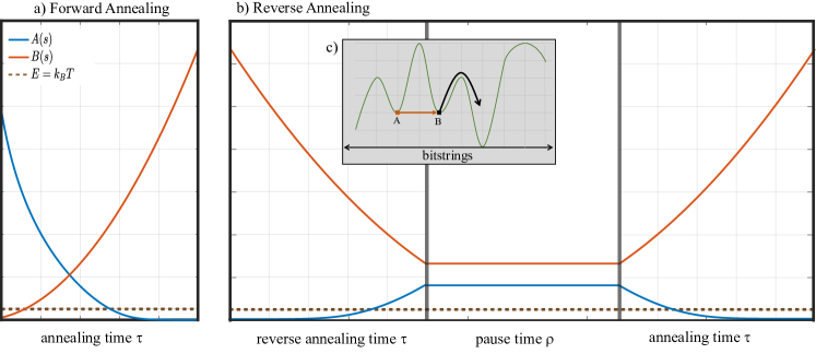
Figure 1: Quantum annealing schedules on DW2000Q used in our investigations, with reference to Eq.(7). a) Forward quantum annealing schedule. b) Reverse quantum annealing schedule where the three steps of the protocol are all set to the same duration of $\tau$=$\rho$. c) Pictorial view of what should be facilitated by reverse quantum annealing: when the initial bitstring is a local minimum (A), the reverse protocol should allow tunneling between valleys (A$\rightarrow$B) while the pause should facilitate gradient descent as well as allow for local exploration through thermal hopping (escape from B towards the global minimum).

Reverse Quantum Annealing

Figure 1-b illustrates the quantum annealing protocol when the DW2000Q is set to operate as a reverse annealer. The system is initialized with $B[t]$=$\max{B}$ and $A[t]$=0, with spins set to a classical bitstring $\mathcal{S}$. The evolution then undergoes an inverse schedule illustrated in Figure 1-a up to a point where the Hamiltonian time-dependence is temporarily paused. With reference to the Hamiltonian evolution in Eq.(7), the transverse field evolution that we program for this protocol is the following three-phases function (identical equations for $B^{R}[t]$, $B^{p}[t]$, $B^{F}[t]$ in terms of $B[t]$):

$$A^{R}[t]=A[\tau+(s_{p}-1)t] \textrm{(Reverse Annealing)}\;\;t\in[0,\tau]$$ (8)

$$A^{p}[t]=A[s_{p}\tau] \textrm{(Annealing Pause)}\;\;t\in[\tau,\tau+\rho]$$

$$A^{F}[t]=A[(1-s_{p})(t-\rho)-(1-2s_{p})\tau] \textrm{(Forward Annealing)}\;\;t\in[\tau+\rho,2\tau+\rho]$$

where $\rho$ is the duration of the pause and $s_{p}\in[0,1]$ indicates the location of the forward schedule where the pause is implemented. The total duration of the selected reverse anneal protocol is $2\tau+\rho$ as opposed to $\tau$ for the forward anneal.

While the theory of reverse annealing is just starting to be investigated [24, 25, 26], the physics rationale of reverse annealing is to be found in the oversimplified idea that, if the system is initialized in a state $\mathcal{S}$ corresponding to a local minimum of the objective function (4), the interplay of quantum and thermal fluctuations might help the state tunnel out of the energy trap during the reverse annealing, while the annealing pause (and to some extent the final forward annealing) allows the system to thermalize and relax in the neighborhood of the newfound minimum. See Figure 1-c for a pictorial view of the concept.

The quality of the initial state $\mathcal{S}$ is likely to influence dramatically the reverse annealing process. For our experiments we use a classical greedy algorithm to set $\mathcal{S}$, as described in the next section.

4 Experimental Results

We aim to solve representative portfolio instances at the limit of programmability of the most advanced DW2000Q device, and to benchmark the results by means of a competitive heuristics running on classical computers. Note that due to the embedding overhead on DW2000Q we can embed a maximum of 64 logical binary variables on a fully-connected graph, which means that the largest search space for our benchmarks is around $60!/(30!)^{2}\simeq$ hundred thousand trillion if $M=N/2$. Our instance set consists of 30 randomly generated instances for each of the following number of assets $N=${24, 30, 36, 42, 48, 54, 60}. In Table 2 we show the expected number of assets in the optimal portfolio of our unconstrained problem sets, computed by using all methods in this study, showing that the search space is non-trivial for all tested cases. Since exhaustive search is out of question for the largest problems, we provide two algorithms below that will be used to have a reference benchmark of the DW2000Q results.

A common metric to benchmark performance of non-deterministic iterative heuristics against quantum annealing is Time-to-Solution (TTS). The TTS is defined as the expected number of independent runs of the method in order to find the ground state with probability (confidence level) $\alpha$:

$$\textrm{TTS}=t_{\textrm{run}}\frac{\ln(1-\alpha)}{\ln(1-p)}\;,$$ (9)

where $t_{\textrm{run}}$ is the running time elapsed for a single run (either $\tau$ for forward or $2\tau+\rho$ for reverse), and $p$ is the probability of finding the optimum of the objective function in that single shot [1, 27].

Greedy Search

The simplest reference benchmark to consider is the portfolio obtained with the best $M$ assets, neglecting correlations ($b_{ij}$=0). The second simplest approach is to consider an iterative greedy search where correlations are taken into account progressively starting from the selection/exclusion of the most desirable/undesirable assets. This is implemented for instance by the routine shown in the pseudocode (Algorithm 1) below.

Note that this greedy search is the procedure we use to set the initial state $\mathcal{S}$ for reverse annealing. Table 2 displays results obtained by applying the greedy search algorithm to the unconstrained problem Eq. (2) for the instance set, as a reference point, highlighting the percentage of instances solved with the greedy search heuristic as a function of problem size.

Problem	% of instances solved:		Number of assets	Parameters search space
size	Greedy	Forward	in the optimal
$N$	Search	Annealing	portfolio	$J_{F}$	$s_{p}$	$\rho$ (µs)
24	80%	100%	10 ($-3,+$4)	3-7(0.5)	$-$	$-$
30	90%	100%	12 ($-5,+$7)	3-7(0.5)	$-$	$-$
36	93%	97%	13 ($-7,+$7)	3-7(0.5)	$-$	$-$
42	70%	90%	16 ($-7,+6$)	5-8(0.5)	0.32-0.5(0.02)	1-15(7)
48	47%	87%	17 ($-6,+5$)	5-8(0.5)	0.32-0.5(0.02)	1-15(7)
54	60%	60%	19 ($-7,+12$)	5-8(0.5)	0.32-0.5(0.02)	1-15(7)
60	57%	30%	23 ($-13,+15$)	6-9(0.5)	0.32-0.5(0.02)	1-15(7)

Table 2: Benchmark Instance Set characterization. For the number of assets in the optimal portfolio we report the median and the maximum and minimum in parenthesis, over 30 instances. The parameters search space for optimization of quantum annealing is reported in the last three columns, in the format min-max(step).

Algorithm 1 Greedy Search Heuristic

1:  # Initialize energy tuples with the local magnetic fields, $h$:

2:  for $i$ from 0 to number of qubits $-$ 1 do

3:     $energy[i]$ = $\{-|h(i)|,h(i),i\}$

4:  end for

5:  # Reorder energy tuples into a heap according to absolute magnitude:

6:  $Energies$ = heap($energy$)

7:  # Initialize solutions:

8:  while $Energies$ do

9:     # Energy tuple elements (largest magnitude energy tuple first):

10:     $\{x,e,i\}$ = heappop($Energies$)

11:     if $e>0$ then

12:        $Solution[i]=-1$

13:     else

14:        $Solution[i]=+1$

15:     end if

16:     # Update the rest of the heap:

17:     for $z$ in $Energies$ do

18:        $n=z[2]$ # Qubit number

19:        # Energy update with the coupling strength, $J$:

20:        $z[1]=z[1]+Solution[i]*(J(i,n)+J(n,i))$

21:        $z[0]=-|z[1]|$

22:     end for

23:  end while

Genetic Algorithm

We choose Genetic Algorithm (GA) as a classical benchmark heuristics. Genetic Algorithms are adaptive methods of searching a solution space by applying operators modelled after the natural genetic inheritance and simulating the Darwinian struggle for survival. There is a rich history of GA applications to solving portfolio optimization problems [28, 29], including recent researches [12, 30] that explored a range of new portfolio optimization use cases.

A GA performs a multi-directional search by maintaining a population of proposed solutions (called chromosomes) for a given problem. Each solution is represented in a fixed alphabet with an established meaning (genes). The population undergoes a simulated evolution with relatively good solutions producing offsprings, which subsequently replace the worse ones. The estimate of the quality of a solution is based on a fitness function, which plays role of an environment. The simulation cycle is performed in three basic steps. During the selection step a new population is formed by stochastic sampling (with replacement). Then, some of the members of the newly selected populations recombine. Finally, all new individuals are re-evaluated. The mating process (recombination) is based on the application of two operators: mutation and crossover. Mutation introduces random variability into the population, and crossover exchanges random pieces of two chromosomes in the hope of propagating partial solutions.

In the case of portfolio optimization problem the solution (chromosome) is a vector ${\bf q}=(q_{1},\ldots,q_{N})$ consisting of $N$ elements (genes) that can take binary values $q_{i}\in\{0,1\}$. Our task is to find the combination of genes that minimizes the objective (fitness) function $O({\bf q})$. Due to the relatively short string of genes we do not use the crossover recombination mechanism as it provides very little value in improving the algorithm convergence (see Algorithm 2 for details).

Algorithm 2 Genetic Algorithm $-$ unconstrained portfolio optimization

1:  Generation of $L$ initial solutions by populating the chromosomes through the random draw from the pool of possible gene values {0, 1}.

2:  Evaluation of the objective (fitness) function for each solution.

3:  Ranking of solutions from ’best’ to ’worst’ according to the objective function evaluation results.

4:  for $i$ from 0 to number of iterations $-$ 1 do

5:     Selection of $K$ best solutions from the previous generation and production of $L$ new solutions by randomly changing the values of one or more genes. With $L=mK$ every one of the ’best’ solutions will be used to produce $m$ new solutions.

6:     Evaluation of the objective (fitness) function for each solution.

7:     Ranking of solutions from ’best’ to ’worst’ according to the objective function evaluation results.

8:  end for

The best values of parameters $L$ and $K$ depend on the problem size and specific QUBO coefficient mapping scheme and can be found through the trial and error process. The objective here is to achieve the target convergence with the smallest number of objective function calls. The computational time of a single objective function call on the test machine (Intel(R) Xenon(R) CPU E5-1620 v4 processor run at 20% CPU utilization) has been measured to be proportional to $N^{2}$ up to a cost of about 30 µs for $N=60$.

Note that, as with all heuristics, the GA approach does not guarantee optimality. Hence the scaling measured is not necessarily representative of the complexity of the problem $-$ but rather a measure of the ability of the algorithmic approach to find the best solution.

Optimization of Forward and Reverse Quantum Annealing

As discussed in Section 3, our runs on DW2000Q are fully specified by: an embedded Ising model (5) where the free embedding parameter $J_{F}$ has been set, an annealing time $\tau$, and the pause time $\rho$ and location $s_{p}$ (for reverse annealing). Moreover, in order to obtain meaningful results on the values of the logical variables, a majority voting decoding procedure has been applied to the returned measurements of the physical qubits of the embedded Ising Eq. (5-6) for each 1D chain, as customary [20]. Finally, runs are separated in batches of 1500 anneals each with a different spin-reversal transormation (or ”gauge”) in order to average out systematic errors during the anneals [22].

In order to determine the best parameters, we bruteforce over a fixed set of values (see Table 2), and we measure the TTS for all those parameters, singling-out the lowest found value, instance by instance (see Appendix C). This simple procedure represents a statistical pre-characterization of the instance ensemble sensitivity to the parameters, and it is common for quantum annealing benchmarking initial studies of a problem [3, 20, 31]. Due to the post-selection of the best embedding and pause location parameters, the reported results then will represent a “best case scenario”, however previous empirical research show that once the distribution of typical optimal parameters has been estimated, it is possible to set up a lightweight on-the-fly procedure to set the parameters dynamically while performing the runs [32]. The results of the parameter setting optimization are shown in Figure 2 for forward and reverse annealing. It should be immediately noted that we don’t optimize over $\tau$ since our experiments (as well as prior research on similar instances [31]) indicates that the best TTS is obtained for the fastest annealing time, $\tau$ = 1 µs . What is shown is that the median best choice for $|J_{F}|$ is increasing with the problem size (as expected [20]) and the mean best choice for $s_{p}$ increases with the pause period. With regard to reverse annealing, we should note that we don’t pre-characterize all 30 instances, but only those that have not been solved by the greedy heuristics (Algorithm 1) that is used to initialize the reverse annealing procedure. For those instances we are facing a three-parameter optimization ($|J_{F}|$, $\rho$, $s_{p}$).

Figure 2: Left: Median and distribution of optimal $J_{F}$ as a function of problem size (See Table 2 for ranges of search). Darker colors indicate higher probability (forward quantum annealing results). Right: Mean optimal $s_{p}$ as a function of pause time, $\rho$. Error bars show 1 standard deviation confidence bands. Annealing time $\tau$ was fixed at 1 µs.

What is clear from the results on reverse annealing is that (i) a good guess for the optimal $J_{F}$ parameter is accurately predicted by the value obtained for forward annealing, and (ii) the optimal pause location is consistently later in the anneal for larger $\rho$. The first observation considerably simplifies the parameter setting strategy when considering operational scenarios with a new unknown instance, while the second observation is consistent with recent results and interpretation of the annealing pause tested on native Chimera problems [24].

Results

Figure 3 displays the TTS results for the GA algorithm, the forward QA solver and the reverse QA solver results. Of particular interest of this study are the probability of success obtained for 42-, 48-, 54- and 60-asset portfolios against the forward annealing results obtained for all portfolio sizes. We report also on the comparison with GA - to have a baseline reference on how comparatively perfomant is the quantum solver against a classical CPU. GA can also be initialized by the Greedy Search heuristics, and this also decreases the TTS required for GA to find the global minimum (orange curve in Figure 3).

From the comparisons, the best solver appears to be reverse quantum annealing at minimum annealing time and pause time. In the median case, we observe one to three orders of magnitude speed-up when applying reverse quantum annealing with respect to quantum annealing.

Figure 3: Time-to-solution (99% confidence level): GA, Forward and Reverse Quantum Annealing. Curves follow the median and error bars indicate 30% and 70% percentile over the 30 instances. The TTS curve for Forward QA is limited to $N=54$ since for $N=60$ the median is not well defined, as only 30% of instances solve to the best known objective value. Dashed curves indicate median TTS obtained with higher $\rho$ (no error bars displayed for clarity). All TTS are measured not counting the time required to run the greedy descent that initializes the initial ansatz $\mathcal{S}$, nor the overhead times for operating the DW2000Q (see Discussion in Section 5).

5 Conclusion and Next Steps

In this paper we did investigate a combinatorial optimization problem in Finance, identifying parameters and mappings that are related to real-world portfolio optimization approaches and that are compatible with the precision requirements of current D-Wave machines. The resulting QUBO has integer coefficients and is very densely connected. Hence, we leveraged prior research on fully-connected graphs by employing the state-of-the-art methods to compile the problem on the Chimera architecture.

While for general coefficients the quadratic problem is NP-hard, the instances that we randomly generate are not necessarily hard. As a matter of fact, using the simple greedy pre-processing approach (Algorithm 1) we can solve a large part of them as shown in Table 2. We did not filter on difficulty since we don’t expect all portfolio optimization problems of interests to be hard necessarily, and it is difficult to classify the instances on their expected difficulty beforehand. However, as the number of variables $N$ increases, while QUBO parameters are kept the same, we expect greedy approaches and classical heuristics to fail on typical instances.

Consistently with the rest of the literature, all reported times for runs on the DW2000Q have been calculated in terms of the annealing times $\tau$ (or $\rho$), ignoring all other necessary setup and iteration times, since they don’t scale with the problem size and they could be reduced in the future as system integration of the chips improves. However, once one considers the additional overhead times required to complete a full run on the D-Wave machine, the advantage disappears, and the TTS results are on par with our classical benchmark. It is important to note that the reported scaling of TTS with problem size has not a fundamental character as the parameters that influence TTS ($J_{F}$, $\tau$, $\rho$, $s_{p}$) are optimized only within a limited range. In particular, the annealing time is expected to be suboptimal for $N\leq 50$, leading to a measurement of a flatter slope for the median TTS [33]. While asymptotic scaling analysis can be extrapolated only on future devices that support more variables and parameter values, we believe there is value in reporting on the complexity according to the current operational scenarios.

We note that improvements can be made over our analysis and approach and engineering advances are being planned in the next few years on quantum annealers. For instance, research papers on reverse annealing and paused annealing are just beginning to appear [24, 34], and it seems that for hard problems it might be beneficial to implement a longer pause, larger than 100 microseconds, to gain a sizeable TTS advantage. Moreover, we do not expect difference in probability of success if we were to decrease the forward/reverse anneal time $\tau$ beyond 1 µs, since the process is dominated by thermalization during the pause. Based on these considerations, it is reasonable to believe that more than an order of magnitude of performance can be gained by further tuning the quench time $\tau$ and the pause time $\rho$.

A second very promising development that could also lead to order of magnitudes improvements is the transition of the D-Wave Chimera architecture to the Pegasus architecture. According to forecasts, the next chip will be able to embed almost 400 logical variables, reducing embedding overhead of at least a factor of 3. According to recent research [31] the embedding overhead is responsible for a large part of the performance, hence we expect conservatively to gain at least an order of magnitude from this improvement. Another possible performance enhancement could be coming from inhomogeneous driving [35]. As the number of physical qubits increases, we could also leverage error-suppression encodings nested with embedding [36] that while reducing the total number of logical variables they provably improve the probability of success. Additional knobs available that could improve upon the current TTS are: the use of multiple pauses and the additional precision on the J couplings offered by the extended J-range feature.

Bearing all these considerations in mind, while it is not clear if quantum annealing is going to be the most compelling solver for portfolio optimization, our results indicate that as technology and theory progresses it could represent a viable choice. Our conclusion is indeed that these first results on the use of quantum annealing in reverse mode look very promising, especially in light of the large room for improvement that is possible to achieve by future hardware design.

From a Finance perspective, another direction of future research is to explore alternative portfolio optimization approaches. For example, we can mention here work done by Sortino and van der Meer [37] on skewed return distributions. Sortino ratio that normalizes excess return by the downside deviation often provides more valuable information about relative portfolio performances than widely used Sharpe ratio, where excess return is normalized by the standard deviation of both positive and negative portfolio returns.

Acknowledgements

The collaboration between USRA and Standard Chartered Bank has been supported by the USRA Cycle 3 Program that allowed the use of the D-Wave Quantum Annealer 2000Q^TM, and by funding provided by NSF award No. 1648832 obtained in collaboration with QC-Ware. We acknowledge QC-Ware and specifically thank Eric Berger, for facilitating the collaboration and contributing to the runs on the D-Wave machine. D.V. acknowledges general support from NASA Ames Research Center and useful discussions with QuAIL research team. A.K. would like to thank David Bell and USRA for the opportunity to conduct research on the quantum annealer at QuAIL.

Disclaimer and Declaration of Interest

The authors report no conflict of interest. The authors alone are responsible for the content and writing of the paper. The opinions expressed are those of the authors and do not necessarily reflect the views and policies of Standard Chartered Bank or the Universities Space Research Association. All figures are based on own calculations.

This paper is for information and discussion purposes only and does not constitute either an offer to sell or the solicitation of the offer to buy any security or any financial instrument or enter into any transaction or recommendation to acquire or dispose of any investment.

Appendix A Geometric Brownian Motion

A Geometric Brownian Motion (GBM) is a stochastic process $S(t)$ that satisfies the following stochastic differential equation (SDE):

$$dS(t)=\mu S(t)dt+\sigma S(t)dB(t)\;,$$

where $t$ is continuous time and $B(t)$ is a Brownian motion. GBM is widely used to model asset prices. If a unit of time is 1 year, then $\sigma$ is interpreted as an annualized volatility (standard deviation) of asset’s log-returns, which are assumed to be normally distributed. The drift coefficient $\mu$ controls deterministic component of the asset price process.

Integrating the process we obtain:

$$S(t)=S(0)\exp\left(\left(\mu-\frac{1}{2}\sigma^{2}\right)t+\sigma B(t)\right)\;.$$

Although GBM SDE can be used directly to simulate an asset process, it is better to use its solution to ensure that simulated asset prices do not turn negative $-$ this may be the case for large enough time step. In our portfolio optimization example $\Delta t$ = 1 month and we use the following discretization scheme for a single asset price process:

$$S(t_{n})=S(t_{n-1})\exp\left(\left(\mu-\frac{1}{2}\sigma^{2}\right)\Delta t+\sigma z_{n}\sqrt{\Delta t}\right)\;,$$

where $t_{n}=t_{n-1}+\Delta t$ and $z_{n}$ is a standard normal random variable. Asset prices from the $N$-asset portfolio are jointly simulated using the same scheme but correlated standard normal random variables $(z^{(1)},\ldots,z^{(N)})$ are constructed via Cholesky decomposition of the correlation matrix $\rho$.

Appendix B Chimera Graph of DW2000Q and Embedding

In Figure 4 we show the layout of the chip used for the experiments, belonging to the machine D-Wave 2000Q hosted at NASA Ames Research Center.

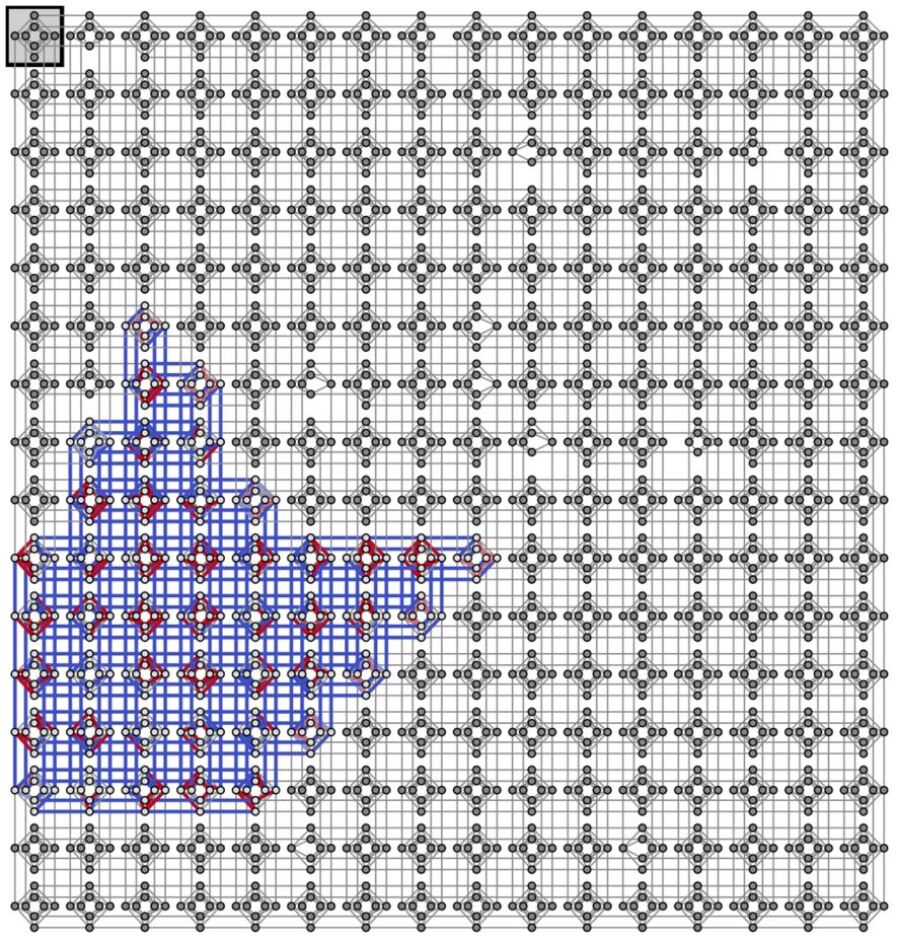
Figure 4: Chimera Chip of DW2000Q. Each gray dot represents an active qubit (missing dots are broken qubits), the black shaded square is representative of one unit cell. The embedding for an instance ($N$=42) is highlighted: blue bonds are ferromagnetic couplings set to $J_{F}$, while red and pink bonds represent logical couplings ($J_{ij}$ in Eq.(6)).

Appendix C More details on parameter setting for Reverse Annealing

Figure 5 displays median TTS results obtained for the mapping schemes provided by Table 1 and annealing times 1 µs and 10 µs, obtained for the first 10 instances of the benchmark ensamble on an independent set of runs with respect to the results presented in Figure 3. It is clear that the choice of $\tau$ = 1 µs is the most advantageous.

Figure 5: Time-to-solution (99% confidence level) for different $t_{\textrm{run}}$ (median over 10 instances).

In Figure 6 we show on an example how the optimal parameter setting is performed to generate data in Figure 2 and 3. Scans are performed for different $J_{F}$ and $s_{p}$ and the best TTS is selected, instance by instance.

Figure 6: Time-to-solution (99% confidence level) as a function of annealing parameter $s_{p}$. Results for a single instance, $N=42$, $\tau$ = 1 µs. Circles point out to the best found ($J_{F}$, $s_{p}$) for these three illustrative cases.

References

- [1] Troels F Rønnow, Zhihui Wang, Joshua Job, Sergio Boixo, Sergei V Isakov, David Wecker, John M Martinis, Daniel A Lidar, and Matthias Troyer. Defining and detecting quantum speedup. Science, 345(6195):420–424, 2014.
- [2] Vasil S Denchev, Sergio Boixo, Sergei V Isakov, Nan Ding, Ryan Babbush, Vadim Smelyanskiy, John Martinis, and Hartmut Neven. What is the computational value of finite-range tunneling? Physical Review X, 6(3):031015, 2016.
- [3] Davide Venturelli, Dominic JJ Marchand, and Galo Rojo. Quantum annealing implementation of job-shop scheduling. arXiv preprint arXiv:1506.08479, 2015.
- [4] Tobias Stollenwerk, Bryan O’Gorman, Davide Venturelli, Salvatore Mandrà, Olga Rodionova, Hok K Ng, Banavar Sridhar, Eleanor G Rieffel, and Rupak Biswas. Quantum annealing applied to de-conflicting optimal trajectories for air traffic management. arXiv preprint arXiv:1711.04889, 2017.
- [5] Alex Mott, Joshua Job, Jean-Roch Vlimant, Daniel Lidar, and Maria Spiropulu. Solving a higgs optimization problem with quantum annealing for machine learning. Nature, 550(7676):375, 2017.
- [6] Johnson, Matthew and Correll, Randall and Giesecke, Kay and McMahon, Peter and Su, Vincent Quantum-Annealing Computer Method for Financial Portfolio Optimization US20170372427A1 QC-Ware Corp. Patent application
- [7] Gili Rosenberg, Poya Haghnegahdar, Phil Goddard, Peter Carr, Kesheng Wu, and Marcos López De Prado. Solving the optimal trading trajectory problem using a quantum annealer. IEEE Journal of Selected Topics in Signal Processing, 10(6):1053–1060, 2016.
- [8] Michael Marzec. Portfolio optimization: applications in quantum computing. Handbook of High-Frequency Trading and Modeling in Finance (John Wiley & Sons, Inc., 2016) pp, pages 73–106, 2016.
- [9] Harry Markowitz. Portfolio selection. The journal of finance, 7(1):77–91, 1952.
- [10] KV Fernando. Practical portfolio optimization. The Numerical Algorithms Group, Ltd White Paper, 2000.
- [11] Hans Kellerer, Renata Mansini, and M Grazia Speranza. Selecting portfolios with fixed costs and minimum transaction lots. Annals of Operations Research, 99(1-4):287–304, 2000.
- [12] Alexei Kondratyev and George Giorgidze. Evolutionary algos for mva optimisation. Risk, 30(12):136–141, 2017.
- [13] William F Sharpe. Mutual fund performance. The Journal of business, 39(1):119–138, 1966.
- [14] John C Hull and Sankarshan Basu. Options, futures, and other derivatives. Pearson Education India, 2016.
- [15] Serge Darolles and Christian Gourieroux. Conditionally fitted sharpe performance with an application to hedge fund rating. Journal of banking & finance, 34(3):578–593, 2010.
- [16] Mark W Johnson, Mohammad HS Amin, Suzanne Gildert, Trevor Lanting, Firas Hamze, Neil Dickson, R Harris, Andrew J Berkley, Jan Johansson, Paul Bunyk, et al. Quantum annealing with manufactured spins. Nature, 473(7346):194, 2011.
- [17] Tony T Tran, Minh Do, Eleanor G Rieffel, Jeremy Frank, Zhihui Wang, Bryan O’Gorman, Davide Venturelli, and J Christopher Beck. A hybrid quantum-classical approach to solving scheduling problems. In Ninth Annual Symposium on Combinatorial Search, 2016.
- [18] Hamed Karimi and Gili Rosenberg. Boosting quantum annealer performance via sample persistence. Quantum Information Processing, 16(7):166, 2017.
- [19] Tomas Boothby, Andrew D King, and Aidan Roy. Fast clique minor generation in chimera qubit connectivity graphs. Quantum Information Processing, 15(1):495–508, 2016.
- [20] Davide Venturelli, Salvatore Mandra, Sergey Knysh, Bryan OǴorman, Rupak Biswas, and Vadim Smelyanskiy. Quantum optimization of fully connected spin glasses. Physical Review X, 5(3):031040, 2015.
- [21] Joshua Job and Daniel Lidar. Test-driving 1000 qubits. Quantum Science and Technology, 3(3):030501, 2018.
- [22] Andrew D King and Catherine C McGeoch. Algorithm engineering for a quantum annealing platform. arXiv preprint arXiv:1410.2628, 2014.
- [23] Sergio Boixo, Vadim N Smelyanskiy, Alireza Shabani, Sergei V Isakov, Mark Dykman, Vasil S Denchev, Mohammad H Amin, Anatoly Yu Smirnov, Masoud Mohseni, and Hartmut Neven. Computational multiqubit tunnelling in programmable quantum annealers. Nature communications, 7:10327, 2016.
- [24] J. Marshall, D. Venturelli, I. Hen, and E. G. Rieffel. The power of pausing: advancing understanding of thermalization in experimental quantum annealers. ArXiv e-prints, October 2018.
- [25] Masaki Ohkuwa, Hidetoshi Nishimori, and Daniel A. Lidar. Reverse annealing for the fully connected -spin model. Phys. Rev. A, 98:022314, Aug 2018.
- [26] Kostyantyn Kechedzhi, Vadim Smelyanskiy, Jarrod R McClean, Vasil S Denchev, Masoud Mohseni, Sergei Isakov, Sergio Boixo, Boris Altshuler, and Hartmut Neven. Efficient population transfer via non-ergodic extended states in quantum spin glass. arXiv preprint arXiv:1807.04792, 2018.
- [27] Salvatore Mandra and Helmut G Katzgraber. A deceptive step towards quantum speedup detection. Quantum Science and Technology, 2018.
- [28] Dan Lin, Xiaoming Li, and Minqiang Li. A genetic algorithm for solving portfolio optimization problems with transaction costs and minimum transaction lots. In International Conference on Natural Computation, pages 808–811. Springer, 2005.
- [29] Kyong Joo Oh, Tae Yoon Kim, and Sungky Min. Using genetic algorithm to support portfolio optimization for index fund management. Expert Systems with Applications, 28(2):371–379, 2005.
- [30] Saranya Kshatriya and P Krishna Prasanna. Genetic algorithm-based portfolio optimization with higher moments in global stock markets. Risk, 20(4):1–26, 2018.
- [31] Ryan Hamerly, Takahiro Inagaki, Peter L McMahon, Davide Venturelli, Alireza Marandi, Tatsuhiro Onodera, Edwin Ng, Carsten Langrock, Kensuke Inaba, Toshimori Honjo, et al. Experimental investigation of performance differences between coherent ising machines and a quantum annealer. arXiv preprint arXiv:1805.05217, 2018.
- [32] Alejandro Perdomo-Ortiz, Joseph Fluegemann, Rupak Biswas, and Vadim N Smelyanskiy. A performance estimator for quantum annealers: Gauge selection and parameter setting. arXiv preprint arXiv:1503.01083, 2015.
- [33] Tameem Albash and Daniel A Lidar. Demonstration of a scaling advantage for a quantum annealer over simulated annealing. Physical Review X, 8(3):031016, 2018.
- [34] Daniele Ottaviani and Alfonso Amendola. Low rank non-negative matrix factorization with d-wave 2000q. arXiv preprint arXiv:1808.08721, 2018.
- [35] Adame, J and McMahon, P. L.. Inhomogeneous driving in quantum annealers can result in orders-of-magnitude improvements in performance. arXiv preprint arXiv:1806.11091, 2018.
- [36] Walter Vinci, Tameem Albash, and Daniel A Lidar. Nested quantum annealing correction. npj Quantum Information, 2:16017, 2016.
- [37] Frank A Sortino and Robert Van Der Meer. Downside risk. Journal of portfolio Management, 17(4):27–31, 1991.