On the possibility of homogeneous nucleation of water droplets and/or ice crystals during the bounces of a cavitation bubble.

Abstract

Acoustic cavitation is known to trigger ice nucleation in supercooled water. Several competing and still debatable mechanisms have been proposed in the literature and are related to the pressure field in the vicinity of the bubble at the end of its collapse. Numerical simulations of the bubble dynamics show that during the bubble expansions in the bounces following the main collapse, the bubble core temperature reaches values far below $0\text{\,}\mathrm{\SIUnitSymbolCelsius}$ for time periods of about $500\text{\,}\mathrm{n}\mathrm{s}$. The water vapour present in the bubble during these time intervals explores the liquid and the solid region of the phase diagrams before going back to the vapour region. On the base of approximate nucleation kinetics calculations, we examine to what extent liquid droplets could nucleate homogenously in the bubble core during these excursions. We also discuss the possibility that the nucleated clusters reach the bubble wall and trigger ice nucleation in the surrounding liquid if the latter is supercooled.

I Introduction

Gas bubbles submitted to a sound field undergo radial oscillations, a phenomenon known as acoustic cavitation. For enough large amplitude of the driving field, such bubbles undergo an explosive growth followed by a rapid collapse. The density energy in the compressed gas at the end of the collapse is large enough to break chemical bounds and produce light emission, known as sonoluminescence.

Cavitation bubbles are also known to trigger ice nucleation in supercooled water. In absence of ultrasound, nucleation is a stochastic process and can occur over a relatively wide range of supercooling temperatures. When subject to even short ultrasound bursts, supercooled water can freeze at lower supercooling level Hem (1967); Hunt and Jackson (1966a); Bhadra (1968); Gitlin and Lin (1969); Inada et al. (2001); Chow et al. (2005); Nakagawa et al. (2006); Lindinger et al. (2007); Saclier et al. (2010). This ability to control the nucleation temperature has interesting and promising industrial applications. Despite various mechanisms have been proposed to explain this effect and several studies report experimental results, the mechanism of ice nucleation by a radially oscillating bubble remains unclear.

Two main available theories have been proposed Hickling (1965, 1994); Hunt and Jackson (1966b); Hunt and Jackson (1966a), and share a common feature: both attribute ice nucleation to a shift of the freezing point in the supercooled liquid phase, because of large pressure variations at the end of the bubble collapse. A large majority of species increase their freezing temperature $T_{f}$ as pressure increases. Normal ice (ice I) constitutes an exception since the solid phase is less dense than the liquid, so that a compression of supercooled water would therefore normally quench freezing. Hickling Hickling (1965) argues that the very large pressures attained (typically several GPa) in the vicinity of the bubble allow the nucleation of ice V, VI and VII, which contrarily to ice I, have a positive $dT_{f}/dp$ slope. Hunt & Jackson notices that the large pressure increase at the end of the collapse is followed by a very high negative transient pressure, which may increase supersaturation relative to ice I nucleation. Both theories are equally mentioned in studies of cavitation-enhanced water freezing. Due to the very short space- and timescales involved, a direct confirmation of one or the other mechanism appears hardly feasible, despite Hickling’s statement has been favored by calculations of orders of magnitude Ohsaka and Trinh (1998).

In the present work, we examine the possibility of a third mechanism, which has been overlooked in past studies. The above-mentioned theories only examine the thermodynamic state of the surrounding water. However, in the curse of the volume oscillations of the bubble, water evaporates and condensates at the interphase, so that the bubble encloses a variable quantity of water vapor. Finite-rate mass diffusion of water vapor through noncondensable gas Storey and Szeri (2000); Toegel et al. (2000) and non-equilibrium evaporation/condensation at the bubble wall Yasui (1997); Colussi and Hoffmann (1999); Storey and Szeri (2000) are known to prevent water from condensing during the collapse. This water-trapping mechanism has been recognized to decrease the final collapse temperature Moss et al. (1999); Yasui (2001); Storey and Szeri (2000), which plays a crucial role in sonoluminescence, and in particular explains the enhancement of single-bubble sonoluminescence (SBSL) in cold water Barber et al. (1994); Vazquez and Putterman (2000); Storey and Szeri (2002); Yasui (2001).

However, poor attention has been paid to the fate of the bubble vapor content after the collapse. A first plausible reason for that is that sonoluminescence and sonochemistry studies are mainly concerned with the hot state of the bubble interior at the end of the collapse, so that the subsequent phases of the bubble dynamics are of little interest in this framework. A second reason is that a bubble is not granted to maintain a spherical shape and even to survive after its collapse in multi-bubble conditions. However, a single bubble in a levitation experiment is shape-stable for millions of cycles in single-bubble experiments Barber et al. (1997); Brenner et al. (2002), and bubbles stable for several cycles have been reported in some multi-bubbles experiments Mettin (2005). This justifies the study of the water vapor content after the main collapse. Of special interest is the re-expanding phase of the bubble after the primary or secondary collapses. A naive examination of the radius-time curve around the collapse shows that the re-expansion also occurs on a timescale almost as fast as the collapse (see for example Fig. 2a). One may therefore expect that, as the collapse yields considerable heating of the bubble interior, the re-expansion might produce a large cooling of the bubble content, including water vapor. The goal of this work is the assess the latter point and to examine its implications on potential nucleation of liquid water droplets or ice crystals. From an historical point of view, this is an attempt to link the long known effect of cavitation on ice nucleation, to more recent theories modeling water and heat transport in an oscillating spherical bubble.

II The state of water vapor during bubble bounces

To calculate the water state in the bubble, we use a simplified model based on thermal and mass diffusion layers popularized by studies on SBSL Toegel et al. (2000); Storey and Szeri (2001), and recently validated against more refined models Stricker et al. (2011). In order to simplify the discussion, we neglect chemical dissociation of the bubble content. The bubble radial dynamics is described by a Keller equation Keller and Kolodner (1956); Prosperetti and Lezzi (1986); Brenner et al. (2002). We study the case of an air bubble in water, at ambient pressure $p_{0}=101300$ Pa, driven at 20 kHz. We first consider a bubble in water at ambient temperature $T_{0}=298$ K, with physical properties of water $\rho_{l}=$ 1000 kg/m³, $\mu_{l}=$ 10^-3 Pa.s, $\sigma=$ 0.0725 N.m^-1

Figure 1 displays the variations of the radius (Fig. 1a) and core temperature (Fig. 1b) of an air bubble of ambient radius $R_{0}=5\>\mu$m, driven by a 20 kHz sinusoidal field of amplitude $p_{a}=130$ kPa. The classical temperature peaks can be observed at the main and secondary collapses. Moreover, an interesting feature of the temperature curve can be observed on Figs 2a-b, which are zoom into Figs 1a-b around the bubble afterbounces: slightly after the main collapse and also after the secondary ones, the bubble core temperature falls down below 0^∘C for a short time during the bubble re-expansion. Although this feature is visible in other works (see for example Fig. 1c in Yasui (1996), Fig. 1d in Yasui (1997), Fig. 4 in Gong and Hart (1998), Fig. 2 in Kim et al. (2007)), to our knowledge, it has never been commented.

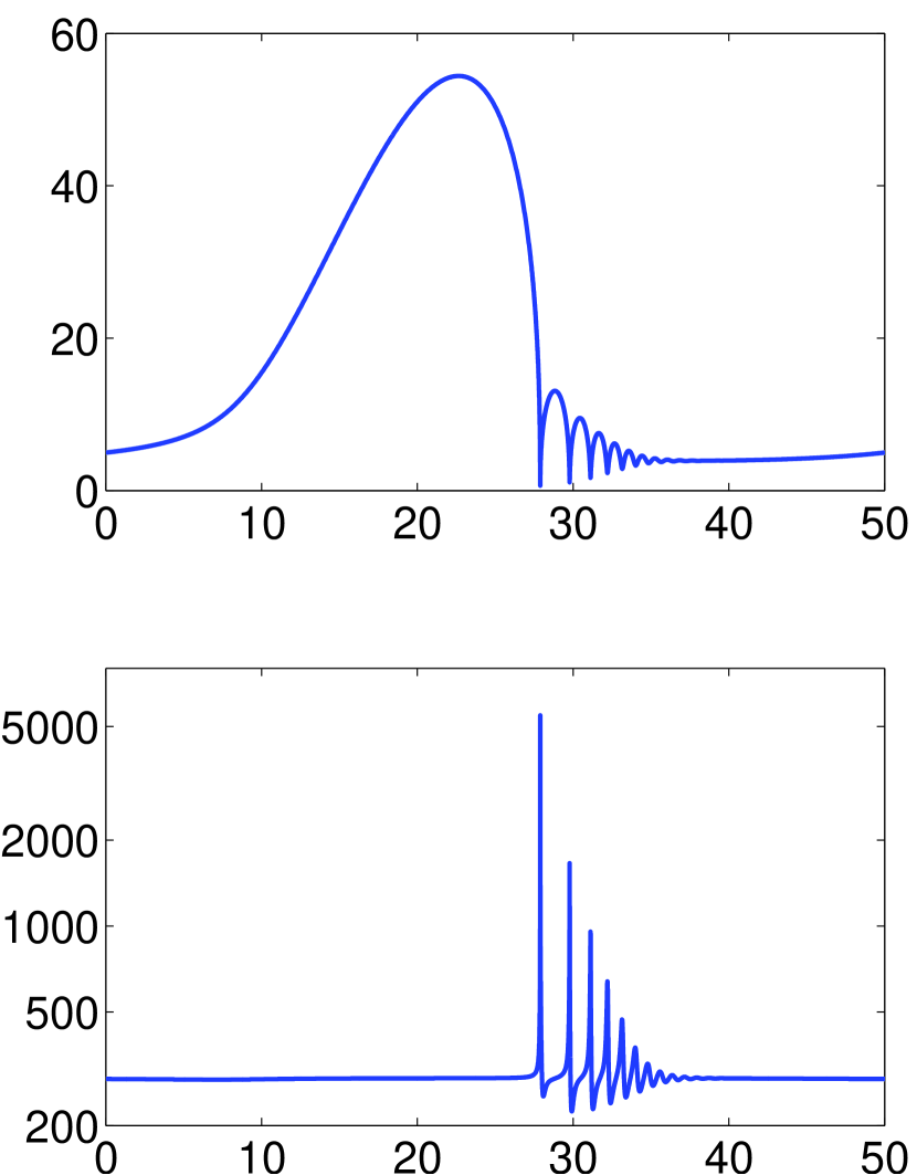
Figure 1: a. Temporal evolution of the radius of a 5 $\mu$m air bubble in water driven by a 20 kHz field at $p_{a}=130$ kPa. b. Temporal evolution of the bubble core temperature.

The physical origin of this feature shares some similarities with the adiabatic heating of the bubble core during the collapse: the expansion velocity is fast enough to partially inhibit heat conduction between the liquid and the bubble core, so that the expansion phases are almost adiabatic.

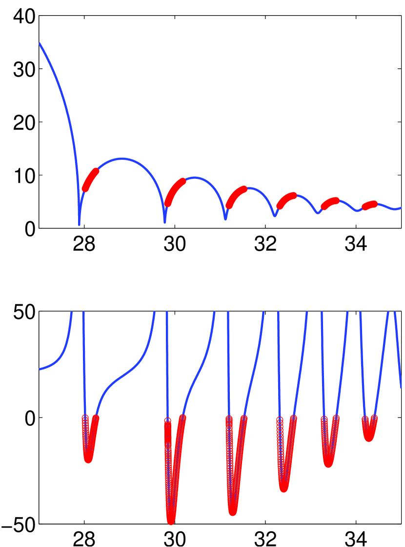
Figure 2: Zoom of Fig. 1 around the collapses. The red (color online) circle marks on both curves materialize the times at which the bubble core is at a temperature below 0^∘C

Moreover, owing to finite diffusion of vapor through air, there is excess water trapped in the bubble core during the bounces, which slowly condenses at the bubble wall from one bounce to the other Storey and Szeri (2000); Toegel et al. (2000). Thus, when the temperature of the bubble core drops below 0^∘C, the water vapor content is cooled down to freezing temperatures. This raises the question of whether this water vapor is thermodynamically stable against liquefaction or ice formation. In order to assess this issue, we first plot the path followed by the state of water in a temperature/water partial pressure phase diagram. Fig. 3 displays a subset of this path around the post-collapse bubble expansions materialized by red circle-marks (color online) on Fig. 2. It can be seen that the vapor state crosses several time the liquid-vapor boundary and even performs six excursions in the solid region, during time periods of hundreds of ns. This timescale, although very short compared to the acoustic period, is much larger than the collapse characteristic time. The partial pressure of water vapor ranges between $10^{3}$ and $10^{4}$ Pa, so that at this scale the liquid-solid boundary is almost the vertical line $T=0^{\circ}$ C. The numbers correspond to the order of appearance in the acoustic cycle, and the paths are described anti-clockwise. The second excursion yields the lowest temperature ($-48.9^{\circ}$ C), as could also be seen in Fig. 2b.

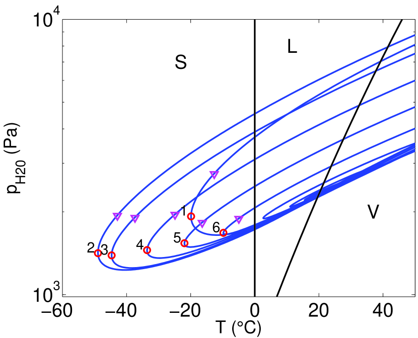
Figure 3: (Color online) Evolution of water conditions in the phase diagram of water $(T,p_{\text{H${}_{2}$O}})$ in the conditions of Fig. 1 (blue thick solid lines). The phase boundaries are drawn in black thin dashed lines. The circles materialize the six negative peak temperatures visible in Fig. 2, numbered by increasing time. The triangles materialize the water vapor state slightly before the minimal temperature is attained, and are represented to illustrate the direction followed by the trajectories. The dashed lines are the boundaries between the vapor, liquid and solid states of water. The excursion of the trajectories in the solid region are, for the paths numbered from 1 to 6: 236 ns, 332 ns, 331 ns, 305 ns, 266 ns, 204 ns.

The present simulation suggests therefore that even in a liquid at ambient temperature, the water vapor of the bubble becomes repeatedly metastable during the bubble bounces, not only against liquefaction, but also against ice formation, for time lapses of about hundreds of ns. This opens the interesting issue of whether this metastable vapor has enough time to nucleate into droplets or ice crystals inside the bubble. Before going further, one should comment on the singularity of the above results, in view of the parameters used for the simulation yielding Figs. 1-3, which are typical of bubbles levitated in SBSL cells. Such bubbles are known to keep their spherical shapes for a large number of cycles, so that they indeed undergo bounces. The present result would thus suggest that inertial single bubbles commonly observed in levitation cells have their content ready for ice nucleation in the expansive part of their bounces, even at room temperature. Whether ice nuclei have indeed enough time to form in such bubbles or not has therefore to be clarified.

If the latter observation also held for a bubble surrounded by supercooled water, this result would provide a new explanation, albeit incomplete, of how cavitation can trigger so easily ice formation in supercooled water. In order to clarify this point, we reproduced the precedent simulation in supercooled water at temperature $T_{L}^{\infty}=-5^{\circ}\>\text{C}$. The path of the water state in the plane ($T$, $p_{\text{H${}_{2}$O}}$) is displayed as a solid line in Fig. 4. The path obtained for $T_{L}^{\infty}=20^{\circ}\>\text{C}$ (as displayed in Fig. 3) is recalled in dashed line for comparison. Several differences can be observed. As expected, the bubble inner temperature is shifted toward low values since the surrounding liquid is colder. It is seen that the minimal temperatures attained during bounces are thus lower than for a bubble at ambient temperature (the minimum temperature attained reaches $-67.5^{\circ}C$ in this case). Moreover, the water vapor pressure is also shifted toward lower values, since the bubble in colder water initially contains less vapor.

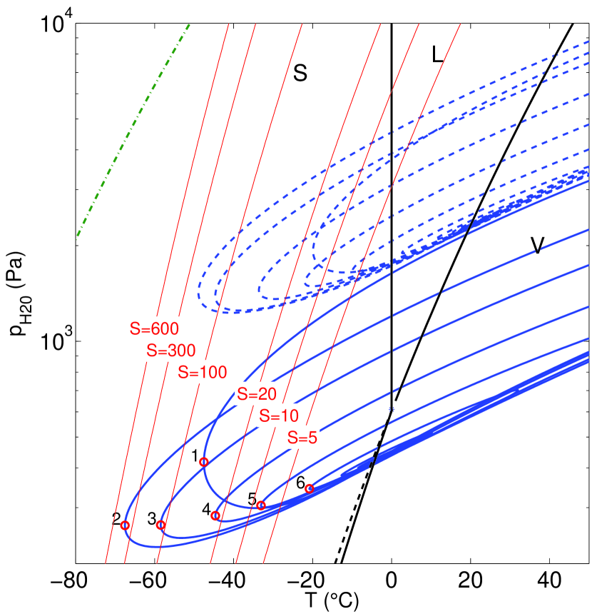
Figure 4: (Color online) Evolution of water conditions in the phase diagram of water $(T,p_{\text{H${}_{2}$O}})$ for a 5 $\mu$m air bubble in water driven by a 20 kHz field at $p_{a}=130$ kPa. Solid (blue) line: $T_{L}^{\infty}=-5^{\circ}\>\text{C}$; Dashed (blue) line: $T_{L}^{\infty}=20^{\circ}\>\text{C}$ (same as Fig. 3). The phase boundaries are drawn in thin dashed (black) lines. The additional thin dashed line starting from the triple point is the equilibrium curve between supercooled water and vapor. There are 10 excursion loops in the solid whose respective durations are 908 ns, 663 ns, 531 ns, 455 ns, 420 ns, 417 ns, 413 ns, 425 ns, 445 ns, and 514 ns. The (red) solid line are the supersaturation ratio level curves from Eq. (1). The (green) dash-dotted line is an estimation of the vapor spinodal line (see appendix A)

Thus, in the case of a bubble surrounded by supercooled water, the water vapor in the bubble is therefore not only metastable against liquefaction, but moreover enters in the temperature range below the so-called homogeneous freezing point of water at -42${}^{\circ}C$, which has long been considered as the supercooling limit for liquid water Angell (1983), below which homogeneous freezing occurs. One might therefore be tempted to conclude that ice should nucleate, at least temporarily in the bubble during the excursions in the solid phase on Fig. 4. Whether freezing indeed occurs inside the bubble is the main question discussed in this paper. We first propose a short review of the abundant literature on water freezing, notably in the context of cloud microphysics, and extending in the more general frame of water physics.

III Review of water freezing

III.1 Cloud physics

The conditions in the bubble are similar to the ones encountered in clouds, and the related issue of the formation of liquid and/or ice in the latter. The state of water in clouds has been recently found to be crucial for climate change predictions, and motivated an active research in this field. Clouds are formed by expansion and cooling of humid air as it ascends, so that vapor becomes thermodynamically unstable and condensation into liquid droplets occurs Debenedetti (1996); Mason (2010). This condensation is favored by the presence of soluble or insoluble aerosol particles called cloud condensation nuclei (CCN) Mason (2010). Formation of ice can occur at moderate negative temperatures by several mechanisms involving specific aerosol particles (called ice forming nuclei, IFN) in low and middle troposphere clouds Cantrell and Heymsfield (2005); Murray et al. (2012). However in high altitude clouds such as cirrus, the dearth of such IFNs prevents such mechanisms and supercooled water droplets can be found down to $-40$ ^∘C Sassen et al. (1985); Sassen (1992); Heymsfield and Miloshevich (1993); Debenedetti (2003). Below this temperature, the supercooled droplets in the cloud freeze homogeneously.

III.2 Water no man’s land

These results are in close agreement with laboratory experiments, which have evidenced the so-called homogeneous freezing temperature $T_{H}$ below which supercooled droplets unavoidably undergo homogeneous freezing. According to classical nucleation theory, this temperature in fact slightly varies with the droplet size, since the number of nucleated embryos per unit time is proportional to the sample volume. At the time of Angell’s early review on supercooled water Angell (1983), the lowest temperature ever reached for supercooled pure water was -42^∘C in micron-sized droplets Mossop (1955).

However, it has been demonstrated that ultra-fast cooling of water allows to bypass homogeneous freezing, and to obtain amorphous ice with a glass transition at 136 K, which further crystallize into cubic ice (Ic) near $150$ K upon heating Debenedetti (2003). There exists therefore a domain between 150 K and 231 K, termed as “no man’s land” Mishima and Stanley (1998), where the existence and properties of supercooled water could not be assessed for long.

Entering the no man’s land has been achieved first by the pioneering work of Bartell and co-workers Bartell and Huang (1994); Huang and Bartell (1995), by expanding a mixture of carrier gas (neon) and water vapor through small supersonic nozzles. With cooling rates of $10^{7}$ K/s, liquid water clusters of 74 Å (6000 molecules) could be observed and analyzed by electron diffraction spectroscopy. The clusters were found to freeze at temperatures as low as 200 K, and diffraction patterns showed that cubic ice (Ic) was nucleated. Similar recent experiments with slightly lower cooling rate ($10^{5}$ K/s) and argon as the carrier gas allowed to nucleate and freeze supercooled droplets between 202 K and 215 K Manka et al. (2012). The estimated homogeneous nucleation rates in supersonic nozzle experiment can reach about $10^{30}$ m^-3s^-1, which is between 15 and 20 orders of magnitude larger than the nucleation rates observed slightly above the no man’s land, where numerous results have been collected Huang and Bartell (1995). In spite if this large range of nucleation rate, models based on classical nucleation theory, and assuming nucleation of cubic ice (Ic), seem to yield rather good results, even if there remains uncertainties on the interfacial energy between liquid and ice (Ic) Murray et al. (2010); Manka et al. (2012).

That deeply supercooled water freezes into cubic ice (Ic) rather than hexagonal ice (Ih) is supported by Bartell’s electron diffraction spectra Bartell and Huang (1994); Huang and Bartell (1995) and by the presence of cubic ice in clouds Riikonen et al. (2000); Goodman et al. (1989). As noted by Murray and co-workers Murray et al. (2012), this also agrees with Ostwald’s rule of stages, which states that the metastable phase nucleate (in this case cubic ice) preferentially to the stable phase (hexagonal ice). Recent experiments, computer simulations, and careful reinterpretations of past studies, revealed that ice formed from supercooled water is in fact composed of randomly stacked layer of cubic and hexagonal sequences Malkin et al. (2012). As noted by Murray and co-workers Murray et al. (2012), the precise phase of the ice critical nucleus remains unknown, and this constitutes an additional difficulty in the establishment of a definitive nucleation theory for supercooled droplets freezing, especially for the estimation of the liquid-solid interfacial energy, which has a huge influence on the nucleation rate. Despite the latter reservations, the freezing rate proposed in Ref. Murray et al. (2010) seems to yield good agreement with a large set of experimental results, over a large range of supercooling, including the no man’s land Manka et al. (2012).

As a final remark on ice nucleation, there seems to have general evidence that direct homogeneous deposition of ice from vapor does not occur, neither in clouds, nor in supersonic expansions experiments Manka et al. (2012). Thus, liquid droplets would always nucleate prior to freezing, which, again, is a consequence of Ostwald’s rule of stages. It sounds therefore reasonable to discard such a mechanism in the present case, and assume that the water vapor in the bubble cannot form ice nuclei without the prior formation of liquid droplets.

III.3 Relevance to the present problem

Following one of the paths visible on Fig. 4, it is seen that the water vapor in the bubble core can be super-cooled to temperatures falling in the no man’s land range. If direct ice deposition from vapor can be discarded, ice formation in the bubble core, if any, could only occur by primary condensation of vapor into droplets, which, further supercooled as the bubble expands, might undergo homogeneous freezing, possibly in the no man’s land region. A reasonable theory for the latter process is available over a wide range of freezing temperatures Murray et al. (2010); Manka et al. (2012). The physics involved is therefore strikingly similar to the one encountered in supersonic nozzles phase transitions. In both cases, the fast cooling of the mixture of water vapor and carrier gas results from an almost adiabatic expansion. The latter owes to a supersonic flow in the nozzle divergent in one case, and by the bubble outward motion in the other.

There remains however the problem of the nucleation of droplets itself. Ultrasonic nozzle experiments Manka et al. (2012) show that droplets first nucleate when supersaturation $p_{\text{H${}_{2}$O}}/p_{\text{sat,liq}}(T)$ reaches a critical value and further grow by condensation of the surrounding vapor. In doing so, heat is released in the carrier gas and increases its temperature, which in turn quenches liquid nucleation, yielding an almost monodisperse aerosol. Once water vapor has almost entirely been consumed, the subsequent expansion in the nozzle cools the droplets until they freeze homogeneously. During the growth phase, droplets are hotter than the surrounding mixture, as vapor condenses at their surface.

Models for this three-step process, droplet nucleation / droplet growth / droplet freezing, are now available and show good agreement with nozzle experiments Hill (1966); Bartell (1990); Sinha et al. (2009); Tanimura et al. (2010). Transposing such models to the present case is technically feasible, by supplementing the ODE set describing the bubble motion with the ODEs describing the droplets nucleation and growth. This would require however to reconsider the thermal model for the bubble interior and add a source term accounting for the heat released by vapor condensation. Embarking in such a procedure is out of the scope of the present paper.

Nevertheless, it is interesting to investigate at least the first step along a given bubble bounce, to assess whether a significant number of droplets can be nucleated, their sizes, and the fraction of the vapor available in the bubble core that is condensed into clusters. Before carrying out these nucleation calculations, we must make sure that spinodal liquefaction of water vapor in the bubble can be discarded in the present case. As can be seen on Fig. 4, the paths followed by water in the $(T,p_{\text{H${}_{2}$O}})$ plane remain sufficiently far from the estimated vapor spinodal line (dash-dotted line), whose estimation is deferred to appendix A. This ensures that condensation of liquid water in the bubble, if any, can only occur through homogeneous droplet nucleation.

IV Kinetics of droplets nucleation

IV.1 Nucleation model

The instantaneous supersaturation ratio related to the vapor-liquid transition is classically defined by:

$$S(p_{\text{H${}_{2}$O}},T)=\frac{p_{\text{H${}_{2}$O}}}{p_{\text{sat,liq}}(T)}$$ (1)

where $p_{\text{sat,liq}}(T)$ is the equilibrium vapor pressure at temperature $T$. As we are dealing with potentially supercooled water, the correlation used for the latter must extend into the deeply supercooled regime, and we use the results of Ref. Murphy and Koop (2005). On the other hand, it should be emphasized that $p_{\text{H${}_{2}$O}}$ is not constant in our case, because the bubble continuously exchanges water with the surrounding liquid phase through its interface. This is why, contrarily to most studies, the supersaturation ratio does not depend on $T$ only.

The evolution of $S$ on the second rebound is displayed on Fig. 5 in the two cases corresponding to Fig. 4: $T_{L}^{\infty}=-5^{\circ}\>\text{C}$ ( solid line, blue online) and $T_{L}^{\infty}=20^{\circ}\>\text{C}$ (dashed line, red online). We also displayed the iso-S curves in the ($T,p_{\text{H${}_{2}$O}})$ plane in Fig. 4 (red online).

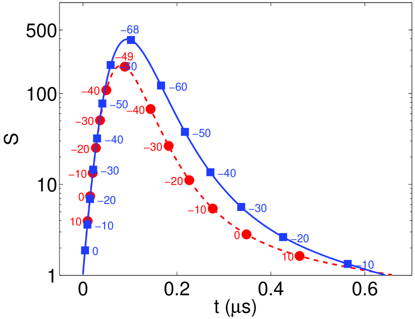
Figure 5: (Color online) Supersaturation ratio in a 5 $\mu$m air bubble in water driven by a 20 kHz field at $p_{a}=130$ kPa, along the second bounce. The conditions are the ones of Fig. 4. The origin of time is chosen when the water vapor state crosses the liquid-vapor equilibrium curve in each case. The markers on the curves indicate the bubble core temperature in ^∘C.

The classical nucleation theory (CNT) Kashchiev (2000) assumes that nucleation occurs through progressive build-up of clusters of molecules, that are precursors of the new phase. A ${g}$-sized cluster can yield a $({g}+1)$-sized cluster by attachment to a water molecule (termed as “monomer”), and conversely the latter can loose a monomer by the backward reaction:

$$({g})+(1)\begin{array}[]{c}\rightharpoonup\\ \leftharpoondown\end{array}({g}+1),\qquad g=1,2,\dots$$ (2)

Under the so-called capillary approximation, the formation energy of a ${g}$-sized cluster can be written as

$$W({g})=kT\left(\Theta{g}^{2/3}-{g}\ln S\right),\qquad\Theta=\frac{a\sigma}{kT}$$ (3)

where $a$ is the area of a monomer, $\sigma$ is the interfacial free energy between the bulk phases, and $\Theta$ its dimensionless form. Assuming spherical clusters, $a=(36\pi v_{0}^{2})^{1/3}$, where $v_{0}$ is the molecular volume.

The energy of formation has a maximum $W^{*}$, which is the nucleation barrier, for a cluster of critical size ${g}^{*}$, defined by :

$$W^{*}=\frac{4}{27}\frac{\Theta^{3}}{(\ln S)^{2}}kT\,\qquad{g}^{*}=\left(\frac{2}{3}\frac{\Theta}{\ln S}\right)^{3},$$ (4)

so that the nucleation rate is essentially the rate of production of critical clusters. Assuming that the cluster size $g$ is a continuous variable, the kinetics of the reaction set (2) can be described by a standard balance equation:

$$\frac{\partial f({g},t)}{\partial t}=-\frac{\partial J({g},t)}{\partial{g}},$$ (5)

where $f({g},t)$ is the concentration in ${g}$-sized clusters and $J({g},t)$ is the cluster flux along the cluster size axis $({g})$. This flux can be shown to read:

$$J({g},t)=-\beta({g},t)f({g},t)\frac{\partial}{\partial g}\left[\frac{f({g},t)}{f_{\text{eq}}({g},t)}\right],$$ (6)

where $\beta({g},t)$ is the attachment rate by collisions between monomers in concentrations $f(1,t)$ and a ${g}$-sized cluster:

$$\beta({g},t)=f(1,t)ag^{2/3}\left(\frac{kT}{2\pi m}\right)^{1/2}$$

with $m$ mass of a water molecule. The quantity $f_{\text{eq}}({g},t)$ is the so-called equilibrium concentration of clusters deduced from the law of mass action.

The correct expression for the latter has been a matter of debate Kashchiev (2000) since the initial work of Becker and Döring Becker and Döring (1935). We use the self-consistent expression proposed by Girshick and co-workers Girshick and Chiu (1990); Girshick et al. (1990); Kashchiev (2006), which, contrarily to the classical formulation, has the advantage to be valid for ${g}=1$:

$$f_{\text{eq}}({g},t)=f_{\text{eq}}(1,t)\exp\left[-\frac{W({g})-W(1)}{kT}\right]$$ (7)

The set of equations (5)-(6) is known as master equation of nucleation. It has no analytic solution in the general case of time-dependent supersaturation, as in the present problem. In particular, as far as we are aware, analytic treatment of the number of nuclei produced by a supersaturation pulse has been poorly explored. A noticeable exception can be found in the work of Trinkaus & Yoo Trinkaus and Yoo (1987) who used Green functions formalism to derive approximate analytic solutions of the master equation, in the case of an idealized nucleation barrier whose location has a parabolic time-dependence around a minimum ${g}^{*}(t)$. However, the analytic expressions proposed by these authors is restricted to the case where the system is still supersaturated when the supersaturation pulse has relaxed, which is not the case here. We must therefore revert to some approximation. The two solutions adopted are described hereafter.

We first note that the simpler problem of transient nucleation in response to a supersaturation step has been extensively studied Kashchiev (1969); Shi et al. (1990); Demo and Kožíšek (1993); Kashchiev (2000). In this case, the transient duration is of the order of the so-called nucleation time lag:

$$\tau=\frac{\delta^{2}}{2\beta({g}^{*})},$$ (8)

where

$$\delta=\left.\left(-\frac{1}{2kT}\frac{\partial^{2}W}{{\partial{g}}^{2}}\right)^{-1/2}\right|_{{g}={g}^{*}}=3{{g}^{*}}^{2/3}\Theta^{-1/2}$$ (9)

is the width of the nucleation barrier. The time-lag is physically the order of magnitude of the time required for the clusters to populate the subcritical region ${g}<{g}^{*}$ by fluctuations.

IV.2 Quasi stationary nucleation rate

If supersaturation has been maintained constant for a duration sufficiently larger than the time-lag, nucleation can be considered stationary, and $\partial f({g},t)/\partial t=0$. Under some approximations, Eq. (5) can then be solved to obtain the steady-state cluster concentration Kashchiev (2000). The stationary nucleation rate $J_{S}$ is defined as the cluster flux through the critical size $J({g}^{*})$ and is found to write:

$$J_{S} = \left(\frac{2\sigma}{\pi m}\right)^{1/2}\left(\frac{p_{\text{sat,liq}}(T)}{kT}\right)^{2}v_{0}e^{\Theta}S$$ (10)

$$\quad\times\exp\left(-\frac{4}{27}\frac{\Theta^{3}}{(\ln S)^{2}}\right).$$

We calculated the latter quantity along the second bounce, in the conditions of Fig. 4, for a liquid at ambient temperature and for a supercooled liquid at $T_{L}^{\infty}=-5^{\circ}\>\text{C}$ (Fig. 6). In both cases, the nucleation rate increases sharply and reaches a maximum after about 100 ns after entering in the metastable liquid zone. The main difference is that both the nucleation rate and the temperature drop much more slowly in the bubble surrounded by the supercooled liquid. On the other hand, a counter-intuitive result is that the maximum nucleation rate is lower for the bubble in the supercooled liquid. This is mainly due to the pre-factor $(p_{\text{sat}}/(kT))^{2}$ which is lower for the supercooled bubble because there is less vapor in the latter (see Fig. 4).

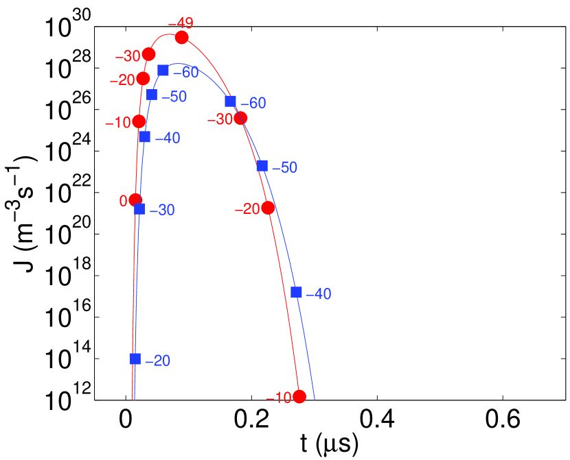
Figure 6: (Color online) Stationary nucleation rate of droplets in a 5 $\mu$m air bubble in water driven by a 20 kHz field at $p_{a}=130$ kPa, along the second bounce, calculated from Eq. (10). Square symbols (blue online): $T_{L}^{\infty}=-5^{\circ}\>\text{C}$; Round symbols (red online): $T_{L}^{\infty}=20^{\circ}\>\text{C}$ (same as Fig. 3). The origin of time is chosen when the water vapor state crosses the liquid-vapor equilibrium curve in each case. The markers on the curves indicate the bubble core temperature in ^∘C.

As proposed by Kashchiev Kashchiev (1970, 2000); Trinkaus and Yoo (1987), the nucleation rate Eq. (10) can still be used if supersaturation evolves on a time scale much larger than the time-lag, a situation referred to as quasi-stationary nucleation. Assuming this assumption valid in our case, the number of critical nuclei formed at time $t$ can be expressed as:

$$N^{\text{QS}}(t)=\int_{0}^{t}J_{S}\bigl{[}S(s),T(s)\bigr{]}\,V(s)\;ds,$$ (11)

whereas the number of water molecules condensed into nuclei reads:

$$n^{\text{QS}}(t)=\int_{0}^{t}J_{S}\bigl{[}S(s),T(s)\bigr{]}\,V(s)\,{g}^{*}(s)\;ds,$$ (12)

In both integrals, the origin of time is chosen when the vapor becomes supersaturated.

In the present case, calculated instantaneous values of the time lag $\tau$ are found to be larger than 1 $\mu$s, except near the supersaturation peak where it becomes of the order of 100 ns. It has therefore the same order of magnitude as the typical time scale of the supersaturation variations, so that the assumption of quasi-stationary nucleation may be not fully reliable here. For a given change of the supersaturation value, nucleation does not reach steady state, and the use of Eqs. (11) probably yields an overestimation of the number of nuclei formed.

IV.3 Transient nucleation

The second method used is to revert to some treatment of transient nucleation in response to a supersaturation step. In the present case, supersaturation evolves rather as a dome-shaped pulse, and a turnaround must be used. Since the rise of $S(t)$ is very abrupt, we replace it by a square pulse between $t_{0}$ and $t_{F}$, defined as (see Fig. 7). The latter times are chosen such that $J_{S}(t_{0})=J_{S}(t_{F})=\alpha J_{S}^{\text{max}}$, where $\alpha$ is a free parameter.

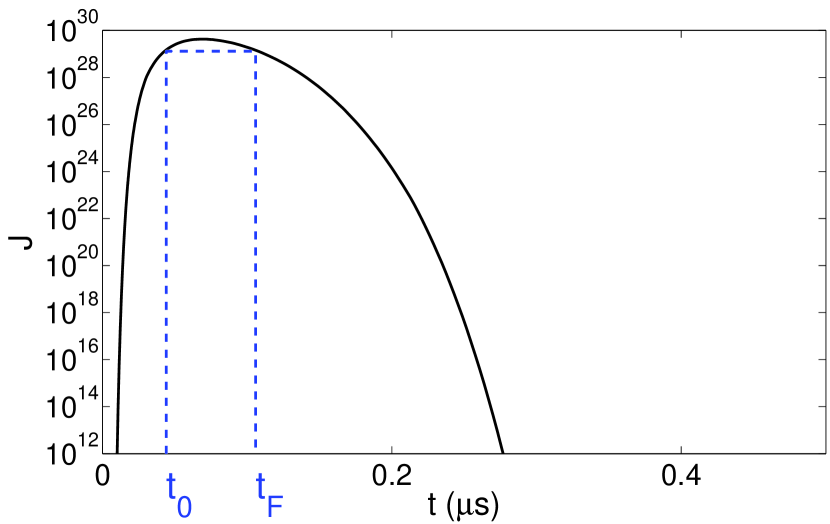
Figure 7: Choice of start-time $t_{0}$ and end-time $t_{F}$ to apply the transient nucleation results of Shi et al. (1990). The values are chosen so that the stationnary nucleation rate $J_{S}$ lies in the range $\alpha J_{S}^{\text{max}}\leq J_{S}\leq J_{S}^{\text{max}}$, where $\alpha$ is a free parameter of order 1 (typically $\alpha=1/2$, see text and Tab. IV.4)

If we restrict our analysis to times lower than $t_{F}$, all happens as if the system had undergone a supersaturation step at $t_{0}$, and classical results of transient nucleation can be used up to time $t_{F}$. The main drawback of the method is that the choice of times $t_{0}$ and $t_{F}$ is somewhat arbitrary, and the sensitivity of the results to this parameter will be examined a posteriori.

We then used the results of Shi, Seinfeld & Okuyama Shi et al. (1990), who used a combination of a boundary-layer method and Laplace transform to solve the nucleation master equation (5) for a supersaturation step at $t=0$. They obtained an analytic expression of the instantaneous cluster size distribution :

$$\frac{f({g},t)}{f_{\text{eq}}({g})} = \frac{1}{2}\textrm{erfc}\left[\frac{{g}-{g}^{*}}{\delta}+\exp\left(-\frac{t}{\tau}+\lambda\right)\right]$$ (13)

$$\qquad-\frac{1}{2}\textrm{erfc}\left[\frac{{g}-{g}^{*}}{\delta}+e^{\lambda}\right],$$

where

$$\lambda={{g}^{*}}^{-1/3}-1+\ln\left[3{g}^{*}\frac{1-{{g}^{*}}^{-1/3}}{\delta}\right].$$ (14)

The concentration of nuclei produced

$$F(t)=\int_{0}^{t}J({g}^{*},s)\;ds$$

was also obtained in analytic form by the authors as:

$$F(t)=J_{S}\frac{\tau}{2}\left[E_{1}(e^{2(\lambda-t/\tau)})-E_{1}(e^{2\lambda})\right],$$ (15)

where $J_{S}$ is the stationary nucleation rate given by Eq. (10), $\tau$ is the nucleation time lag from Eq. (8), and $E_{1}$ is the exponential integral.

In order to use these analytic results, we set the quantities ${g}^{*}$, $\delta$ and $\tau$ to their values at $t_{0}$ and replace $t$ by $t-t_{0}$, up to $t_{F}-t_{0}$. The total number of nuclei $N(t)=\int_{t_{0}}^{t_{F}}J(s)V(s)ds$ formed in the bubble was then approximated by:

$$N^{\text{TRANS}}(t)\simeq F(t-t_{0})V_{m},\qquad t_{0}<t<t_{F}$$ (16)

with $F$ given by Eq. (15), and $V_{m}$ is the mean volume of the bubble during the equivalent supersaturation pulse between $t_{0}$ and $t_{F}$. The number of water molecules condensed into critical nuclei reads similarly:

$$n^{\text{TRANS}}(t)\simeq F(t-t_{0})V_{m}{g}^{*},\qquad t_{0}<t<t_{F}$$ (17)

Since we replaced the exact dome-shaped supersaturation pulse by a smaller square pulse, these estimations are expected to yield lower bounds of the number of nuclei produced and the number of molecules consumed, respectively.

IV.4 Results

Figure 8 displays the number of nuclei produced, $N^{\text{TRANS}}(t)$ from Eq. (16) (thin solid lines) and $N^{\text{QS}}(t)$ from (11) (thick solid lines), in the conditions of Figs. 4-6. The curves for the bubble in ambient water $T_{L}^{\infty}=20^{\circ}\>\text{C}$ end with round symbols (red line online), and the one in supercooled water $T_{L}^{\infty}=-5^{\circ}\>\text{C}$ with square symbols (blue online). The times $t_{0}$ and $t_{F}$ have been chosen on the criterion $J_{S}(t_{0})=J_{S}(t_{F})=\frac{1}{2}J_{S}^{\text{max}}$. The two estimations are expected to yield lower and upper boundaries, respectively, of the number of liquid nuclei formed in the bubble. The number of nuclei obtained at $t_{F}$ in the two cases are displayed as bold lines in Tab. IV.4. As expected from the comparisons of the nucleation rates on Fig. 6, less nuclei are produced in the bubble surrounded by supercooled water.

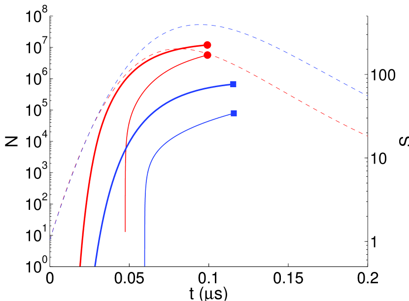
Figure 8: (Color online) Number of nuclei produced during the supersaturation pulse; Thick solid lines: assuming quasi-stationary nucleation ; Thin solid lines: assuming transient nucleation. The conditions are the same as in fig. 6. Square symbols (blue online): $T_{L}^{\infty}=-5^{\circ}\>\text{C}$; Round symbols (red online): $T_{L}^{\infty}=20^{\circ}\>\text{C}$ (same as Fig. 3). The supersaturation is recalled in dashed lines (right ordinate axis) for the two conditions.

We can also make use of Eqs.(12)-(17) to calculate upper and lower bounds for the number of water molecules that have clusterized into nuclei, or more eloquent, the fraction $x$ of those molecules relative to the initial number of water molecules in the bubble as the vapor becomes supersaturated (rightmost columns of Tab. IV.4). It can be seen that during the second rebound of the bubble surrounded by liquid at ambient temperature, between 5 % and 10 % of the water vapor initially present can clusterize into droplets. This fraction drops down to between 0.35 % and 2.5 % in the case of a bubble in supercooled water.

$R_{0}$	$p_{a}$	$T_{L}^{\infty}$	$\displaystyle\alpha=\frac{J_{\text{cut}}}{J_{\text{max}}}$	$N^{\text{TRANS}}$	$N^{\text{QS}}$	$x^{\text{TRANS}}$	$x^{\text{QS}}$
$\mu$m	kPa	∘C				%	%
5	130	-5	1/2	$\mathbf{7.8\times 10^{4}}$	$\mathbf{6.7\times 10^{5}}$	0.35	2.5
5	140	-5	1/2	$7.5\times 10^{4}$	$6.5\times 10^{5}$	0.32	2.5
5	150	-5	1/2	$7.1\times 10^{4}$	$6.4\times 10^{5}$	0.31	2.4
5	130	20	1/2	$\mathbf{5.7\times 10^{6}}$	$\mathbf{1.2\times 10^{7}}$	5.6	10.
5	140	20	1/2	$4.9\times 10^{6}$	$1.1\times 10^{7}$	4.7	9.3
5	150	20	1/2	$4.2\times 10^{6}$	$1.0\times 10^{7}$	3.9	8.3

5 & 130 -5 1/3 $6.5\times 10^{4}$ $7.2\times 10^{5}$ 0.32 2.8 5 140 -5 1/3 $6.5\times 10^{4}$ $7.1\times 10^{5}$ 0.31 2.7 5 150 -5 1/3 $5.9\times 10^{4}$ $6.9\times 10^{5}$ 0.28 2.6 5 130 20 1/3 $5.0\times 10^{6}$ $1.3\times 10^{7}$ 5.5 11. 5 140 20 1/3 $4.5\times 10^{6}$ $1.2\times 10^{7}$ 4.7 9.9 5 150 20 1/3 $4.2\times 10^{6}$ $1.1\times 10^{7}$ 4.2 9.0

Table 1: Number of clusters created and number of water molecules consumed during the buble second rebound, for various bubble ambient radii and driving pressure amplitudes. The calculation have been performed twice for each parameter set, using $\alpha=1/2$ and $\alpha=1/3$, respectively (see Fig. 7). The two bold lines correspond to the data displayed on Fig. 8

Table IV.4 also displays results obtained for larger driving acoustic pressures. It can be seen that increasing the driving decreases the number of nuclei formed. This is due to the fact that larger driving amplitudes produce hotter collapses, so that the initial temperature at the beginning of the rebounds becomes larger. Thus, vapor supersaturation decreases and so does the nucleation rate.

Finally, we also varied the arbitrary factor $\alpha$ used to define the equivalent supersaturation step (see Fig. 7) in order to assess the sensitivity of the results to this quantity. Table IV.4 shows that the latter is reasonably weak.

A last useful information is the evolution of the cluster size distribution during the supersaturation pulse. The size distribution non-dimensionalized by the equilibrium distribution $f({g},t)/f_{\text{eq}}({g})$ calculated from Eq. (13), is displayed on Fig. 9a, for metastable water at $T_{L}^{\infty}=-5^{\circ}\>\text{C}$ in the same conditions as Fig. 5, for 10 equidistant times covering the supersaturation pulse (thin lines). The classical steady-state $\mathop{\rm erfc}\nolimits$ function is also displayed in thick solid line and the critical size is materialized by the vertical dashed line. It can be clearly seen that the steady-state is not reached, which demonstrates that the latter assumption would be difficult to justify in the present problem.

Another interesting result is the order of magnitude of the largest cluster formed in the bubble during the supersaturation pulse. The number of clusters of each size formed in the bubble was calculated by:

$${\mathcal{N}}({g},t)=f({g},t)V_{m}$$

where $f$ was estimated from Eq. (13), and $V_{m}$ is the mean volume of the bubble during the equivalent supersaturation pulse. The result is displayed as thin lines on Fig. 9b (time increasing from bottom to top). The largest cluster formed is seen to reach only a dozen of monomers.

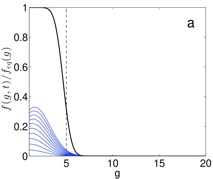
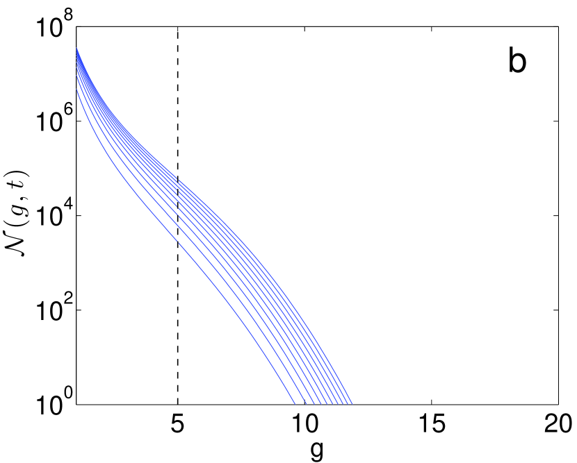
Figure 9: a. Thin lines: dimensionless cluster size distribution calculated from (13) at ten equidistant times covering the supersaturation pulse (time increasing from bottom to top). The thick line represents the number of clusters formed in steady state. b. Number of clusters formed in the bubble.

V Discussion

Using a classical reduced model of bubble dynamics including heat and mass transfer, we have shown that in typical inertial cavitation conditions at 20 kHz, the water vapor in an air bubble becomes strongly metastable during the bubble second rebound, both against liquefaction and freezing. Approximate nucleation calculations show that vapor-liquid phase transition indeed takes place and that a few percents of the initial water content clusterize during the supersaturation pulse. However, owing to the huge supersaturation level, the critical size is about 5 molecules and the largest cluster formed reaches roughly 10 molecules. It is therefore difficult to conclude to the formation of real droplets, in contrast with the experiments in supersonic expansion, where clusters of several thousands molecules are formed, and have additional time to freeze homogeneously. This is due to the typical time scales involved in the respective experiments: the full process in nozzles lasts for about tens of microseconds, whereas the metastable state of the vapor in the bubble lingers for less than 1 $\mu$s (see caption of Fig. 4). Since nucleation is a kinetic process, it cannot proceed efficiently over such a small timescale.

Homogeneous freezing of such small liquid clusters is therefore very unlikely and the scheme of ice crystals nucleating inside the bubble, as was initially suggested by Fig. 4 must be abandoned. However, the fate of the small clusters formed remains an interesting issue. As supersaturation decreases after the peak, one may expect these clusters to dissociate back to monomers (after about 600 ns in the case of Fig. 5). This short lifetime casts some doubts on their ability to redisperse in the surrounding liquid. We note however that the same issue can be raised about the redispersion of the radicals produced by water sonolysis during the bubble collapse, in the frame of sonochemistry. Indeed, such radicals are also short-lived species whose precise mechanism of redispersion in the liquid after the bubble collapse remains unclear. In spite of this lack of knowledge, the entrance of OH^∘ radicals in the liquid is the mechanism commonly put forward to explain their contribution to chemical reactions in the liquid phase. Whether the liquid clusters formed in the bubble are actually able to hit the surrounding liquid pertains to the same questioning. If for the purpose of reasoning, one does not exclude such a mechanism, a highly supercooled liquid cluster coming into contact with the surrounding supercooled liquid might act as a pre-existing entity able to trigger freezing. All would happen as if some part of the surrounding supercooled liquid (typically at $T_{L}^{\infty}=-5^{\circ}\>\text{C}$) underwent a sudden fluctuation down to minus tens of Celsius. Among the plausible contacting mechanisms, non-symmetrical bubble collapse or bubble coalescence may be invoked. Of course, we do not claim that all bubbles undergo such an event precisely when clusters have formed inside, but that such an event has a nonzero probability over billions of bubbles collapsing 20000 times per second. The whole process constitutes an alternative explanation of the ability of cavitation to trigger freezing in supercooled liquids.

Whatever the existence of such a process, the large cooling of the gas/vapor mixture during the bubble rebounds constitutes an interesting and, as far as the authors are aware, unreported feature of acoustic cavitation. More complete models of the bubble interior based on direct Navier-Stokes simulations Storey and Szeri (2000) would be required to confirm and quantify more precisely the reached level of supercooling. If the answer is affirmative, the cavitation bubble would (again) constitute a rather uncommon physical object, whose content is able to cool down to temperatures seldom encountered for water vapor, after having heated up to thousands of Kelvins.

Appendix A Calculation of the vapor spinodal curve

The vapor spinodal curve is generally poorly documented in thermodynamic database. We use therefore the approach of Kim and co-workers Kim et al. (2004) who assumed that the ratio $p_{\text{spinodal}}(T/T_{C})/p_{\text{sat}}(T/T_{C})$ for the fluid of interest was the same as that obtained for an equation of state (EOS) describing a hard sphere fluid corrected by an attractive Yukawa potential Li and Wilemski (2003). We recall the main lines of calculations in this appendix.

The fluid pressure and chemical potential are given respectively by the EOS:

$$p(\rho) = \rho kT\frac{1+\eta+\eta^{2}-\eta^{3}}{\left(1-\eta\right)^{3}}-\frac{1}{2}\alpha\rho^{2},$$ (18)

$$\mu_{(}\rho) = kT\left[\ln\eta+\frac{8\eta-9\eta^{2}+3\eta^{3}}{\left(1-\eta\right)^{3}}\right]-\alpha\rho,$$ (19)

where $\rho$ is the molecular density, $\eta=\pi\sigma^{3}\rho/6$ is the packing fraction, $\sigma$ is the hard sphere diameter, and $\alpha$ is the amplitude of the attractive potential. The corresponding dimensionless critical density $\rho_{C}$ and critical temperature $T_{C}$ are found to be:

$$\rho_{C}\sigma^{3}=6/\pi\eta_{C}=0.24913\quad\text{and}\quad T_{C}=\frac{\alpha}{11.1016\;k\sigma^{3}}.$$

The binodal curve is calculated by solving simultaneously

$$\mu(T,\rho_{l}^{\text{sat}}) = \mu(T,\rho_{v}^{\text{sat}}),$$

$$p(T,\rho_{l}^{\text{sat}}) = p(T,\rho_{v}^{\text{sat}}),$$

for the equilibrium densities $\rho_{l}^{\text{sat}}$ and $\rho_{v}^{\text{sat}}$, and the liquid and vapor spinodal $\rho_{l}^{\text{spin}}$ and $\rho_{v}^{\text{spin}}$ densities are the roots of:

$$\left(\frac{\partial\mu}{\partial\rho}\right)_{T}=0.$$

The equilibrium curve and the two spinodal curves in the $(p,T)$ plane are then obtained by applying the EOS  (18) to the values obtained. The equilibrium and vapor spinodal curves obtained are displayed as thick lines on Fig. 10, and the H₂O equilibrium curve from Ref. Murphy and Koop (2005) used in this paper in thin solid line. We then assume the real vapor spinodal curve to be:

$$p_{\text{spinodal}}=p_{\text{sat}}\frac{p_{\text{spinodal}}^{\text{Yukawa}}}{p_{\text{sat}}^{\text{Yukawa}}}$$ (20)

where $p_{\text{sat}}$ is the vapor pressure calculated from Ref. Murphy and Koop (2005). Figure 10 displays the predicted binodal (thin solid line) and spinodal (thin dashed line) of the hard-sphere Yukawa equation of state. The binodal of Ref. Murphy and Koop (2005) used throughout this paper is represented by a thick solid line and the spinodal deduced from Eq. (20) by a thick dashed line. The latter results displays reasonable agreement with the theoretical prediction of Ref. Dobbins et al. (1988) (square symbols).

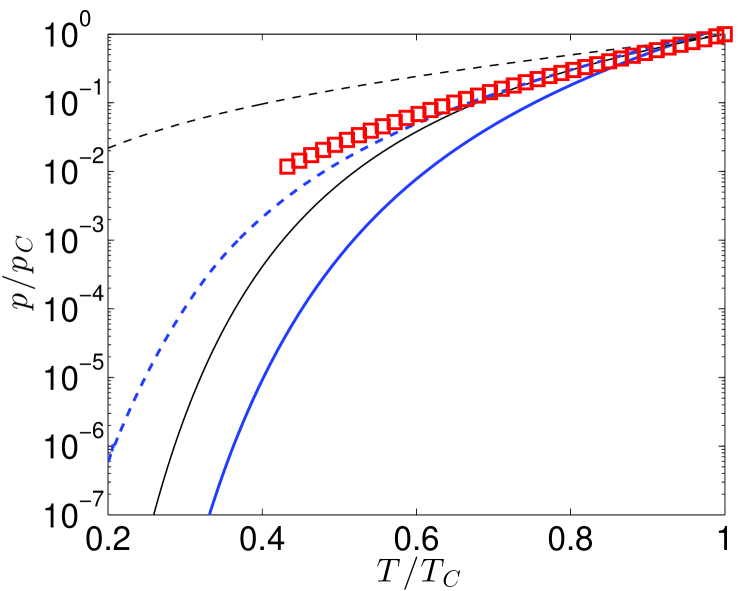
Figure 10: (Color online) Thin (black) lines: vapor pressure curve (solid) and vapor spinodal curve (dashed) calculated from hard sphere/Yukawa EOS (18)-(19). Thick (blue) solid line: vapor pressure of water used in this paper Murphy and Koop (2005). Thick (blue) dashed line: corrected vapor spinodal estimated from (20). The (red) square symbols are the vapor spinodal data for water tabulated in Ref. Dobbins et al. (1988)

References

- Hem (1967) S. L. Hem, Ultrasonics 5, 202 (1967).
- Hunt and Jackson (1966a) J. D. Hunt and K. A. Jackson, Nature 211, 1080 (1966a).
- Bhadra (1968) T. Bhadra, Indian J. Phys. 42, 91 (1968).
- Gitlin and Lin (1969) S. N. Gitlin and S. S. Lin, J. Appl. Phys. 40, 4761 (1969).
- Inada et al. (2001) T. Inada, X. Zhang, A. Yabe, and Y. Kozawa, Int. J. Heat Mass Transfer 44, 4523 (2001).
- Chow et al. (2005) R. Chow, R. Blindt, R. Chivers, and M. Povey, Ultrasonics 43, 227 (2005).
- Nakagawa et al. (2006) K. Nakagawa, A. Hottot, S. Vessot, and J. Andrieu, Chem. Eng. Proc. 45, 783 (2006).
- Lindinger et al. (2007) B. Lindinger, R. Mettin, R. Chow, and W. Lauterborn, Phys. Rev. Lett. 99, 045701 (2007).
- Saclier et al. (2010) M. Saclier, R. Peczalski, and J. Andrieu, Chem. Eng. Sci. 65, 3064 (2010).
- Hickling (1965) R. Hickling, Nature 206, 915 (1965).
- Hickling (1994) R. Hickling, Phys. Rev. Lett. 273, 2853 (1994).
- Hunt and Jackson (1966b) J. D. Hunt and K. A. Jackson, J. Appl. Phys. 37, 254 (1966b).
- Ohsaka and Trinh (1998) K. Ohsaka and E. H. Trinh, Appl. Phys. Lett. 73, 129 (1998).
- Storey and Szeri (2000) B. D. Storey and A. Szeri, Proc. R. Soc. London, Ser. A 456, 1685 (2000).
- Toegel et al. (2000) R. Toegel, B. Gompf, R. Pecha, and D. Lohse, Phys. Rev. Lett. 85, 3165 (2000).
- Yasui (1997) K. Yasui, Phys. Rev. E 56, 6750 (1997).
- Colussi and Hoffmann (1999) A. J. Colussi and M. R. Hoffmann, ”J. Phys. Chem. A”, 103, 11336 (1999).
- Moss et al. (1999) W. C. Moss, D. A. Young, A. David, J. A. Harte, J. L. Levatin, B. F. Rozsnyai, G. B. Zimmerman, and I. H. Zimmerman, pre 59, 2986 (1999).
- Yasui (2001) K. Yasui, Phys. Rev. E 64, 1 (2001).
- Barber et al. (1994) B. P. Barber, C. C. Wu, R. Löfstedt, P. H. Roberts, and S. J. Putterman, Phys. Rev. Lett. 72, 1380 (1994).
- Vazquez and Putterman (2000) G. E. Vazquez and S. J. Putterman, Phys. Rev. Lett. 85, 3037 (2000).
- Storey and Szeri (2002) B. D. Storey and A. J. Szeri, Phys. Rev. Lett. 88, 074301 (2002).
- Barber et al. (1997) B. P. Barber, R. A. Hiller, R. Löfstedt, S. J. Putterman, and K. R. Weninger, Phys. Rep. 281, 65 (1997).
- Brenner et al. (2002) M. P. Brenner, S. Hilgenfeldt, and D. Lohse, Rev. Mod. Phys. 74, 425 (2002).
- Mettin (2005) R. Mettin, in Bubble and Particle Dynamics in Acoustic Fields: Modern Trends and Applications, edited by A. A. Doinikov (Research Signpost, Kerala (India), 2005), pp. 1–36.
- Storey and Szeri (2001) B. D. Storey and A. Szeri, Proc. R. Soc. London, Ser. A 457, 1685 (2001).
- Stricker et al. (2011) L. Stricker, A. Prosperetti, and D. Lohse, J. Acoust. Soc. Am. 130, 3243 (2011).
- Keller and Kolodner (1956) J. B. Keller and I. I. Kolodner, J. Appl. Phys. 27, 1152 (1956).
- Prosperetti and Lezzi (1986) A. Prosperetti and A. Lezzi, J. Fluid Mech. 168, 457 (1986).
- Yasui (1996) K. Yasui, J. Phys. Soc. Japan 65, 2830 (1996).
- Gong and Hart (1998) C. Gong and D. P. Hart, J. Acoust. Soc. Am. 104, 2675 (1998).
- Kim et al. (2007) K. Y. Kim, K. T. Byun, and H. Y. Kwak, Chem. Eng. Sci. 132, 125 (2007).
- Angell (1983) C. A. Angell, Ann. Rev. Phys. Chem. 34, 593 (1983).
- Debenedetti (1996) P. G. Debenedetti, Metastable liquids: concepts and principles (Princeton University Press, 1996).
- Mason (2010) B. J. Mason, Physics of clouds (Clarendon Press, 2010).
- Cantrell and Heymsfield (2005) W. Cantrell and A. Heymsfield, B. Am. Meteorol. Soc. 86 (2005).
- Murray et al. (2012) B. J. Murray, D. O’Sullivan, J. D. Atkinson, and M. E. Webb, Chem. Soc. Rev. 41, 6519 (2012).
- Sassen et al. (1985) K. Sassen, K. N. Liou, S. Kinne, and M. Griffin, Science 227, 411 (1985).
- Sassen (1992) K. Sassen, Science 257, 516 (1992).
- Heymsfield and Miloshevich (1993) A. J. Heymsfield and L. M. Miloshevich, J. Atm. Sci. 50, 2335 (1993).
- Debenedetti (2003) P. G. Debenedetti, Journal of Physics: Condensed Matter 15, R1669 (2003).
- Mossop (1955) S. C. Mossop, Proc. Phys. Soc. B 68, 193 (1955).
- Mishima and Stanley (1998) O. Mishima and H. E. Stanley, Nature 396, 329 (1998).
- Bartell and Huang (1994) L. S. Bartell and J. Huang, J. Phys. Chem. 98, 7455 (1994).
- Huang and Bartell (1995) J. Huang and L. S. Bartell, J. Phys. Chem. 99, 3924 (1995).
- Manka et al. (2012) A. Manka, H. Pathak, S. Tanimura, J. Wolk, R. Strey, and B. E. Wyslouzil, Phys. Chem. Chem. Phys. 14, 4505 (2012).
- Murray et al. (2010) B. J. Murray, S. L. Broadley, T. W. Wilson, S. J. Bull, R. H. Wills, H. K. Christenson, and E. J. Murray, Phys. Chem. Chem. Phys. 12, 10380 (2010).
- Riikonen et al. (2000) M. Riikonen, M. Sillanpää, L. Virta, D. Sullivan, J. Moilanen, and I. Luukkonen, Applied optics 39, 6080 (2000).
- Goodman et al. (1989) J. Goodman, O. B. Toon, R. F. Pueschel, K. G. Snetsinger, and S. Verma, J. Geophys. Res. Atmos. 94, 16449 (1989).
- Malkin et al. (2012) T. L. Malkin, B. J. Murray, A. V. Brukhno, J. Anwar, and C. G. Salzmann, P. Natl. Acad. Sci. 109, 1041 (2012).
- Hill (1966) P. G. Hill, J. Fluid Mech. 25, 593 (1966).
- Bartell (1990) L. S. Bartell, J. of Phys. Chem. 94, 5102 (1990).
- Sinha et al. (2009) S. Sinha, B. E. Wyslouzil, and G. Wilemski, Aerosol Science and Technology 43, 9 (2009).
- Tanimura et al. (2010) S. Tanimura, B. E. Wyslouzil, and G. Wilemski, J. Chem. Phys. 132, 144301 (2010).
- Murphy and Koop (2005) D. M. Murphy and T. Koop, Q. J. R. Meteorol. Soc. 131, 1539 (2005).
- Kashchiev (2000) D. Kashchiev, Nucleation : Basic theory with applications (Butterworths-Heinemann, Oxford, 2000).
- Becker and Döring (1935) R. Becker and W. Döring, Ann. Phys. 24, 719 (1935).
- Girshick and Chiu (1990) S. L. Girshick and C.-P. Chiu, J. Chem. Phys. 93, 1273 (1990).
- Girshick et al. (1990) S. L. Girshick, C. P. Chiu, and P. H. McMurry, Aerosol Sci. Technol. pp. 465–477 (1990).
- Kashchiev (2006) D. Kashchiev, J. Chem. Phys. 125, 044505 (2006).
- Trinkaus and Yoo (1987) H. Trinkaus and M. H. Yoo, Philos. Mag. A 55, 269 (1987).
- Kashchiev (1969) D. Kashchiev, Surf. Sci. 14, 209 (1969).
- Shi et al. (1990) G. Shi, J. H. Seinfeld, and K. Okuyama, Phys. Rev. A 41, 2101 (1990).
- Demo and Kožíšek (1993) P. Demo and Z. Kožíšek, Phys. Rev. B 48, 3620 (1993).
- Kashchiev (1970) D. Kashchiev, Surf. Sci. 22, 319 (1970).
- Kim et al. (2004) Y. J. Kim, B. E. Wyslouzil, G. Wilemski, J. Wölk, and R. Strey, J. Phys. Chem. A 108, 4365 (2004).
- Li and Wilemski (2003) J. S. Li and G. Wilemski, J. Chem. Phys. 118, 2845 (2003).
- Dobbins et al. (1988) R. A. Dobbins, K. Mohammed, and D. A. Sullivan, Journal of physical and chemical reference data 17, 1 (1988).
- Shi and Seinfeld (1994) F. G. Shi and J. H. Seinfeld, Mater. Chem. Phys. 37, 1 (1994).