Investigation of the exchange-correlation potential of functionals based on the adiabatic connection interpolation

Abstract

We have studied the correlation potentials produced by various adiabatic connection models (ACM) for several atoms and molecules. The results have been compared to accurate reference potentials (coupled cluster and quantum Monte Carlo results) as well as to state-of-the-art ab initio DFT approaches. We have found that all the ACMs yield correlation potentials that exhibit a correct behavior, quite resembling scaled second-order Görling-Levy (GL2) potentials, and including most of the physically meaningful features of the accurate reference data. The behavior and contribution of the strong-interaction limit potentials has also been investigated and discussed.

1 Introduction

The study of the exchange-correlation (XC) functional and the development of efficient and accurate approx- imations to it are among the main research topics in density functional theory (DFT). Within this theoreti- cal framework, the XC functional describes in fact all the quantum effects of the electron-electron interaction and it finally determines the accuracy of the overall com- putational procedure.

Over the years many different XC approximations have been developed ^{1, 2} and they are conventionally organized on the so called Jacob’s ladder of DFT ³. To the highest rung of the ladder belong functionals that depend on the Kohn-Sham orbitals and eigenvalues. Some examples of these are the random-phase approximation ^{4, 5}, double-hybrids functionals ^{6, 7} and the ab initio DFT methods ^{8, 9, 10}.

Another class of high-level XC approximations is the one of functionals based on interpolating the adiabatic connection integrand between its weak and strong-interaction limits. These functionals use as starting point the adiabatic connection formula ^{11, 12, 13, 14}

$$E_{xc}=\int_{0}^{1}W_{\lambda}[\rho]d\lambda\ ,$$ (1)

where $\rho$ is the electron density, $\lambda$ is the interaction strength, and $W_{\lambda}[\rho]=\langle\Psi_{\lambda}[\rho]|\hat{V}_{ee}|\Psi_{\lambda}[\rho]\rangle-U[\rho]$ is the density-fixed linear adiabatic connection integrand, with $\Psi_{\lambda}[\rho]$ being the wave function that minimizes $\hat{T}+\lambda\hat{V}_{ee}$ while yielding the density $\rho$ ($\hat{T}$ and $\hat{V}_{ee}$ are the kinetic and electron-electron interaction operators, respectively), and $U[\rho]$ being the Hartree energy. The task of constructing an XC approximation is then translated to the one of developing a proper approximation for the density-fixed linear adiabatic connection integrand $W_{\lambda}$ ¹⁵ by interpolating between its known exact asymptotic behaviors in the weak- and strong-interaction limits ^{16, 17, 18, 19}, i.e.

$$W_{\lambda\rightarrow 0}[\rho] \sim W_{0}[\rho]+\lambda W^{\prime}_{0}[\rho]+\cdots$$ (2)

$$W_{\lambda\rightarrow\infty}[\rho] \sim W_{\infty}[\rho]+\frac{1}{\sqrt{\lambda}}W^{\prime}_{\infty}[\rho]+\cdots\ ,$$ (3)

with

$$W_{0}[\rho]=E_{x}[\rho]\;,\;W^{\prime}_{0}[\rho]=2\,E_{c}^{\rm GL2}[\rho]\ ,$$ (4)

where $E_{x}$ is the exact exchange, $E_{c}^{\rm GL2}$ is the second-order Görling-Levy (GL2) ¹⁶ correlation energy, $W_{\infty}[\rho]$ is the indirect part of the minimum expectation value of the electron-electron repulsion in a given density ¹⁸, and $W^{\prime}_{\infty}[\rho]$ is the potential energy of coupled zero-point oscillations ¹⁹.

The functionals $W_{\infty}[\rho]$ and $W^{\prime}_{\infty}[\rho]$ have a highly nonlocal density dependence, captured by the strictly-correlated electrons (SCE) limit ^{18, 19, 20}, and their exact evaluation in general cases is a non-trivial problem. Notice that while the form of the leading term $W_{\infty}[\rho]$ in Eq. (3) rests on recent mathematical proofs ^{21, 22}, the zero-point term $W^{\prime}_{\infty}[\rho]$ is a very reasonable conjecture that has been confirmed numerically in simple cases ²³, but lacks a rigorous proof. The $\lambda\to\infty$ functionals can also be approximated by the much cheaper semilocal gradient expansions (GEA) derived within the point-charge-plus-continuum (PC) model ²⁴

$${W}_{\infty}^{\rm PC}[\rho] = \int\left[A\rho^{4/3}(\mathbf{r})+B\frac{|\nabla\rho(\mathbf{r})|^{2}}{\rho^{4/3}(\mathbf{r})}\right]d\mathbf{r}$$ (5)

$${W^{\prime}}_{\infty}^{\rm PC}[\rho] = \int\left[C\rho^{3/2}(\mathbf{r})+D\frac{|\nabla\rho(\mathbf{r})|^{2}}{\rho^{7/6}(\mathbf{r})}\right]d\mathbf{r}\ ,$$ (6)

with $A=-9(4\pi/3)^{1/3}/10$, $B=3[3/(4\pi)]^{1/3}/350$, $C=\sqrt{3\pi}/2$, and $D=-0.028957$. For small atoms, it has been shown that these PC approximations provide energies quite close to the exact SCE values ^{18, 19}. More recently, new approximate functionals inspired to the SCE mathematical structure have been also proposed and tested ^{25, 26, 27}. They retain the non-locality of SCE by using as key ingredient some integrals of the density, and their implementation in a self-consistent scheme is still the object of on-going work.

Different interpolation formulas have been employed to obtain several XC functionals based on the adiabatic connection formalism ^{15, 28, 24, 19, 17, 29, 30}. Some of these functionals have been recently tested against realistic physical chemistry problems in order to investigate their performance and understand the corresponding limitations ^{31, 32, 33}. These functionals are all size-extensive but not size consistent when a system dissociates into fragments of different species. However, it has been recently shown that this size consistency error can be easily corrected at no additional computational cost ³³. All these tests have concerned only the quality of the computed energies, whereas no information has been gathered on the XC potentials delivered by the functionals.

Actually, the XC potential is a very important quantity since it enters directly in the Kohn-Sham equations determining the quality of the Kohn-Sham orbitals and energies as well as the features of the electron density ^{34, 35, 36, 37, 38, 39, 40, 41, 42, 43, 44, 45, 46, 47, 48, 49, 50, 51, 52}. Thus, any accurate XC approximation should be able to yield not only precise energies at given densities but also accurate XC potentials. However, this fact is generally overlooked in most investigations of XC approximations, which mainly focus on the energy properties only. On the other hand, a few studies ^{36, 53, 54, 55, 56, 57, 58, 59, 38, 39, 40, 41, 42, 43} have considered the problem of the XC potential showing that an accurate description of both the energy and the potential can be usually achieved only by high-rung approximations (although some important exceptions can be found at the meta-GGA level of theory ^{60, 61}). The ability of an XC functional to describe correctly the XC potential is therefore a significant problem for DFT development.

In this paper, we consider some relevant XC functionals obtained by interpolating between the two limits of Eqs. (2)-(3), studying their ability to describe the XC potential. Obviously, this potential also depends on how the $\lambda\to\infty$ limit of Eq. (3) is approximated. We thus start by comparing the functional derivative of the PC model for the leading term, $W_{\infty}^{\rm PC}[\rho]$ of Eq. (6), with the one from the exact SCE formalism for small atoms. Since the PC model is a GEA (and not a GGA), it diverges far from the nucleus. However, we find that in the energetically important region, the PC functional derivative is a rather good approximation of the SCE potential, at least when evaluated on a given reference density (self-consistently the two will give very different results ^{62, 20, 63}). Moreover, because (due to the $\lambda\to 0$ expansion) all the considered approximations are complicated non-linear functionals of the Kohn-Sham orbitals and eigenvalues, full self-consistent calculations have not been possible, regardless of how the $\lambda\to\infty$ limit is treated. Thus, as explained in the next section, the XC potentials have been computed for fixed reference densities and compared to accurate reference potentials as well as to the second-order Görling-Levy one. This approach was already successfully utilized in some studies ^{64, 35} to investigate the XC potentials properties. Although the procedure does not provide access to the final self-consistent Kohn-Sham orbitals and density, it allows anyway to study the quality of the potential and the ability of each functional to reproduce its most relevant features. This work is therefore a fundamental first step towards the possible full self-consistent implementation of adiabatic-connection-based XC functionals.

2 Potentials from Adiabatic Connection Models

In this work we consider XC functionals based on different adiabatic connection models (ACMs) that use the input quantities of Eqs. (2)-(3), namely the exact exchange $E_{x}$, the second-order Görling-Levy correlation energy $E_{c}^{\rm GL2}$, the strong-interaction limit of the density-fixed adiabatic connection integrand $W_{\infty}$, and possibly the zero-point term $W^{\prime}_{\infty}$. In a compact notation, the XC functionals can be denoted as

$$E_{xc}^{\rm ACM}=f^{\rm ACM}(E_{x},E_{c}^{\rm GL2},W_{\infty},W^{\prime}_{\infty})\ ,$$ (7)

where $f^{\rm ACM}$ is an appropriate non-linear function for the given ACM model. The exact expressions of the $f^{\rm ACM}$ functions corresponding to the functionals considered in this work, namely ISI ¹⁵, revISI ¹⁹, SPL ¹⁷, and LB ²⁹, are given in Appendix. Notice that ISI and revISI depend on all four input quantities while SPL and LB do not depend on $W^{\prime}_{\infty}$. The XC potential corresponding to the functionals defined by Eq. (7) is

$$v_{xc}^{\rm ACM}(\mathbf{r}) \equiv \frac{\delta E_{xc}^{\rm ACM}}{\delta\rho(\mathbf{r})}=$$

$$= D^{\rm ACM}_{E_{x}}\frac{\delta E_{x}}{\delta\rho(\mathbf{r})}+D^{\rm ACM}_{E_{c}^{\rm GL2}}\frac{\delta E_{c}^{\rm GL2}}{\delta\rho(\mathbf{r})}+$$

$$+D^{\rm ACM}_{W_{\infty}}\frac{\delta W_{\infty}}{\delta\rho(\mathbf{r})}+D^{\rm ACM}_{W^{\prime}_{\infty}}\frac{\delta W^{\prime}_{\infty}}{\delta\rho(\mathbf{r})}$$

$$= D^{\rm ACM}_{E_{x}}v_{x}(\mathbf{r})+D^{\rm ACM}_{E_{c}^{\rm GL2}}v_{c}^{\rm GL2}(\mathbf{r})+$$

$$+D^{\rm ACM}_{W_{\infty}}\frac{\delta W_{\infty}}{\delta\rho(\mathbf{r})}+D^{\rm ACM}_{W^{\prime}_{\infty}}\frac{\delta W^{\prime}_{\infty}}{\delta\rho(\mathbf{r})}\ ,$$

where

$$D^{\rm ACM}_{E_{x}}=\frac{\partial f^{\rm ACM}}{\partial E_{x}}\;,\;D^{\rm ACM}_{E_{c}^{\rm GL2}}=\frac{\partial f^{\rm ACM}}{\partial E_{c}^{\rm GL2}}\;,$$ (9)

$$D^{\rm ACM}_{W_{\infty}}=\frac{\partial f^{\rm ACM}}{\partial W_{\infty}}\;,\;D^{\rm ACM}_{W^{\prime}_{\infty}}=\frac{\partial f^{\rm ACM}}{\partial W^{\prime}_{\infty}}\;,$$ (10)

and we used the short-hand notations

$$v_{x}(\mathbf{r})=\frac{\delta E_{x}}{\delta\rho(\mathbf{r})}\;,\;v_{c}^{\rm GL2}(\mathbf{r})=\frac{\delta E_{c}^{\rm GL2}}{\delta\rho(\mathbf{r})}\ .$$ (11)

For the functionals not depending on $W^{\prime}_{\infty}$, i.e. SPL and LB, we have $D^{\rm ACM}_{W^{\prime}_{\infty}}=0$. The derivatives of Eqs. (9) and (10) are straightforward once the function $f^{\rm ACM}$ is fixed. The potentials $\delta W_{\infty}/\delta\rho$ and $\delta W^{\prime}_{\infty}/\delta\rho$ depend on how the $\lambda\to\infty$ limit is treated. For the PC model, they are standard gradient expansion functional derivatives (see Appendix). For the exact case, they can be computed by integrating the SCE force equation ^{18, 62, 20}, see the subsection on the potentials for the strong-interaction limit below.

2.1 Potentials for the weak-interaction limit

The calculations of $v_{x}$ and $v_{c}^{\rm GL2}$ require some attention. In this work we have used the optimized effective potential (OEP) method ^{54, 65}. Then, the potential $v_{x}$ or $v_{c}^{\rm GL2}$ (denoted with general notation $v$ in Eq. (12)) is given by the solution of the integral equation

$$\int\chi(\mathbf{r},\mathbf{r}^{\prime})v(\mathbf{r}^{\prime})d\mathbf{r}^{\prime}=\Lambda(\mathbf{r})\ ,$$ (12)

where $\chi(\mathbf{r},\mathbf{r}^{\prime})$ is the static linear-response function and

$$\Lambda(\mathbf{r}) = \sum_{p}\left[\int\phi_{p}(\mathbf{r})\frac{\delta E}{\delta\phi_{p}(\mathbf{r})}\sum_{q\neq p}\frac{\phi_{q}(\mathbf{r})\phi_{q}(\mathbf{r}^{\prime})}{\epsilon_{p}-\epsilon_{q}}d\mathbf{r}^{\prime}\right.$$ (13)

$$\quad\quad+\left.\frac{\delta E}{\delta\epsilon_{p}}|\phi_{p}(\mathbf{r})|^{2}\right]\ ,$$

with $E$ being either the exact exchange or the second-order Görling-Levy correlation energies, $\phi_{p}$ and $\epsilon_{p}$ being the Kohn-Sham orbitals and orbital energies, respectively. A similar approach was used in Ref. ⁷, leading to the fully self-consistent solution of double-hybrid functionals.

2.2 Computational details

In our study we have considered several atoms, He, Be, Ne, and Ar, the H${}_{2}^{-}$ and F^- ions, as well as the H₂ and N₂ molecules. For all these systems we have determined the self-consistent exact exchange orbitals and density. Exact exchange potential calculations have been carried out with a locally modified version of the ACESII code ⁶⁶ using an uncontracted cc-pVTZ basis set ⁶⁷ for H₂ and N₂, a 20s10p2d basis set ⁶⁸ for He, an uncontracted ROOS-ATZP basis set ⁶⁹ for H, Be, Ne, and F, and for the Ar atom a modified basis set combining $s$- and $p$-type basis functions from the uncontracted ROOS-ATZP ⁶⁹ with $d$- and $f$-type functions coming from the uncontracted aug-cc-pwCVQZ basis set ^{53, 70}. The choice of the basis set was mostly dictated by the need to ensure the best possible expansion for both the wave functions and the OEP potential. For more details see Refs. ^{55, 54}. SUccessively we have computed, in a post-SCF fashion, the XC potentials of the various ACM XC functionals (ISI ¹⁵, revISI ¹⁹, SPL ¹⁷, and LB ²⁹; see Appendix) using Eq. (2). Similarly we have computed, in a one-step procedure based on exact exchange orbitals, the GL2 potential as well as the other OEP correlation potentials (OEP2-sc,OEP2-SOSb). In all these potentials the single excited term has been neglected; anyway this is expected to yield a negligible effect on the final result ⁵⁴.

2.3 Potentials for the strong-interaction limit

The exact (or very accurate ⁷¹) functional derivative of $W_{\infty}[\rho]$ can be computed for spherically symmetric densities using the formalism and the procedure described in Refs. ^{18, 63, 71}. The potential is obtained by integrating numerically the force equation

$$\nabla v_{\rm SCE}[\rho](\mathbf{r})=-\sum_{i=2}^{N}\frac{\mathbf{r}-\mathbf{f}_{i}(\mathbf{r};[\rho])}{|\mathbf{r}-\mathbf{f}_{i}(\mathbf{r};[\rho])|^{3}},$$ (14)

where the co-motion functions $\mathbf{f}_{i}(\mathbf{r};[\rho])$, which are highly non-local density functionals, portray the strictly-correlated regime, determining the positions of $N-1$ electrons as functions of the position $\mathbf{r}$ of one of them ^{18, 63, 71}, and the boundary condition $v_{\rm SCE}[\rho](|\mathbf{r}|\to\infty)=0$ is used. Once $v_{\rm SCE}$ of Eq. (14) has been computed, we then have the exact relation ^{62, 71}

$$\frac{\delta W_{\infty}[\rho]}{\delta\rho(\mathbf{r})}\equiv v_{xc}^{\infty}(\mathbf{r})=v_{\rm SCE}(\mathbf{r})-v_{\rm H}(\mathbf{r}),$$ (15)

where $v_{\rm H}(\mathbf{r})$ is the Hartree potential.

We have computed $v_{xc}^{\infty}(\mathbf{r})$ of Eqs. (14)-(15) for H^-, Be, and Ne, for the same densities as described in the Computational Details Section, using the co-motion functions described in Refs. ^{18, 63, 71}, which are exact for $N=2$ and very accurate (or exact) for $N>2$ ⁷¹. Moreover, even when these co-motion functions are not optimal, the functional derivative of the corresponding $W_{\infty}[\rho]$ still obeys Eqs. (14)-(15) ⁷¹.

Figure 1: Comparison between the exact (or very accurate) functional derivative of the leafing term $W_{\infty}[\rho]$ in Eq. (3), computed with the strictly-correlated electrons (SCE) formalism of Eqs. (14)-(15) ^{18, 63, 71}, and the functional derivative of the GEA approximation obtained from the PC model of Eq. (5).

In Figure 1, we compare these exact (or very accurate) $v_{xc}^{\infty}(\mathbf{r})$ with the functional derivative of $W_{\infty}^{\rm PC}[\rho]$ for the three species. We see that, as anticipated, since the PC model is a GEA, it diverges at large internuclear distances, tending to minus infinity (see Appendix for more details), a feature that would further prevent to perform self-consistent calculations. The exact $v_{xc}^{\infty}(\mathbf{r})$, instead, displays the correct asymptotic behavior $\propto-1/r$ ^{18, 62}. Nonetheless, we see that in the region where the density is significantly different from zero, the PC model provides a very decent approximation to the exact $v_{xc}^{\infty}(\mathbf{r})$. In the next sections, we will then use the much cheaper PC potentials, since we will always compute them on a reference density, where they seem to give rather reasonable results (with the exception of the region close and far from the nucleus). This choice has been further validated by comparing for a few cases the potentials obtained from the SPL and LB models using the PC and SCE functional derivatives: in all cases the differences between the two have been found to be very small, of course with the exception of the asymptotic region far from the nucleus.

There is at present no exact result available for the functional derivative of the zero-point term $W_{\infty}^{\prime}[\rho]$, which is the object of an on-going investigation. For this reason, we will use again the PC model, which also yields a potential that diverges, this time going to plus infinity, but only rather far from the nucleus (see Fig. 2 and Appendix for more details).

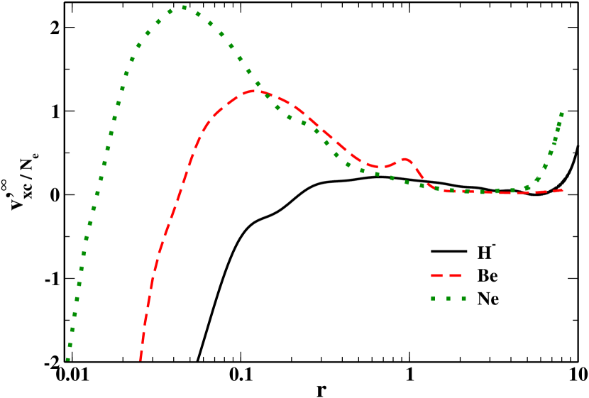
Figure 2: Functional derivative of ${W^{\prime}}_{\infty}[\rho]$, divided by the number of electrons, obtained using the GEA approximation based on the PC model of Eq. (6), for several atoms.

3 Results

In Figure 3 we show the correlation potentials corresponding to different XC functionals (on the scale of the plot ISI and revISI are hardly distinguishable, therefore only the ISI curve has been shown; the same applies to SPL and LB). We recall that all the methods considered in this work include the exchange contribution exactly; therefore only the correlation part of the potential ($v_{c}^{\rm ACM}=v_{xc}^{\rm ACM}-v_{x}$) is of interest for an assessment of the methods. For comparison we have also reported the correlation potential obtained via direct inversion of the coupled cluster single double with perturbative triple (CCSD(T)) density⁷² as well as the one obtained from quantum Monte Carlo (QMC) calculations ^{73, 74}. Both potentials are very accurate and are assumed here as benchmark references. Note anyway that these potentials do not stem from the exact exchange densities used to generate the ACMs potentials, but correspond to self-consistent CCSD(T) or QMC densities. Nevertheless, we expect the difference due to this issue to be almost negligible for the purpose of this work.

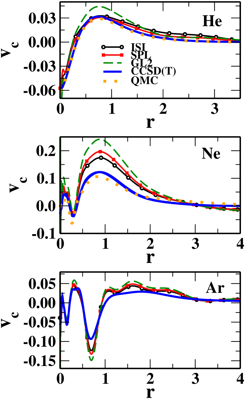
Figure 3: Correlation potentials obtained with different methods for several atoms.

The plots of Fig. 3 show that, in all cases, the various potentials have quite similar shapes. This indicates that for all the ACMs the correlation potential is physically meaningful and describes the main features of the exact potential. Moreover, the ACMs potentials are generally closer to the reference ones than GL2. This latter situation can be measured quantitatively considering the integral error

$$\Delta v_{c}^{\rm ACM}=\int\rho(\mathbf{r})|v_{c}^{\rm ACM}(\mathbf{r})-v_{c}^{Ref}(\mathbf{r})|d\mathbf{r}\ ,$$ (16)

where we use the CCSD(T) potential as reference ($Ref$) and $\rho$ is the exact exchange self-consistent density (i.e. the one used to compute $v_{c}^{\rm ACM}$). The corresponding values are reported in Table 1, whereas a plot of the integrands for the Ne atom case is shown in Fig. 4.

Table 1: Integral error ($\Delta v_{c}^{\rm ACM}$; see Eq. (16)) for different potentials.

	He	Ne	Ar
ISI	0.0088	0.3734	0.1718
revISI	0.0113	0.3136	0.1583
SPL	0.0060	0.5083	0.2123
LB	0.0070	0.5778	0.2258
GL2	0.0212	0.8151	0.2886
OEP2-sc	0.0133	0.1900	0.1062
OEP2-SOSb	0.0170	0.2140	0.1710
OEP2-SOS(opt)	0.0102	0.1127	0.2339

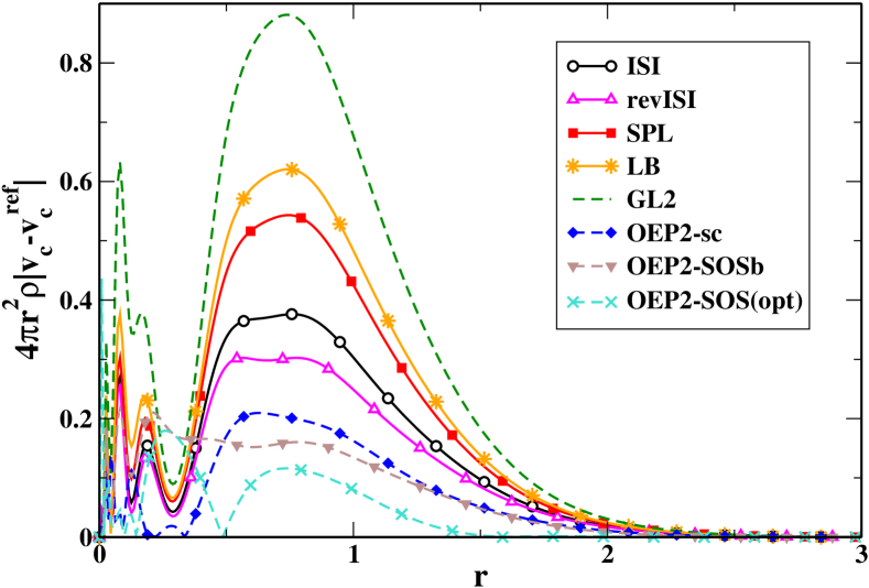
Figure 4: Radial density-weighted absolute errors (see the integrand of Eq. (16)) for various potentials based on adiabatic connection models as well as for GL2 and several second-order OEP potentials, in the case of Ne atom.

These data confirm that the ACMs provide a significant improvement over GL2, yielding values of $\Delta v_{c}^{\rm ACM}$ that are in most cases almost one half that those of GL2. Moreover, the table reports also the integral errors for some accurate second-order OEP methods, namely OEP2-sc ^{8, 10}, OEP2-SOSb ^{54, 55} and OEP2-SOS(opt) ⁵⁵, indicating that the ACMs potentials are competitive with the best available OEP methods. Finally, we find that in general ISI and revISI are slightly better than SPL and LB, most probably due to inclusion of the zero-point term ${W^{\prime}}_{\infty}[\rho]$.

An additional indication of the quality of the ACMs potentials can come by the analysis of the effect they have on the Kohn-Sham orbital energies. In particular, we have considered the first-order perturbative variation of the energy of the highest occupied molecular orbital (HOMO), i.e. $\langle H|v_{c}^{\mathrm{AMC}}|H\rangle$ with $|H\rangle$ being the HOMO state, due to the application of the potential $v_{c}^{\mathrm{AMC}}$. These data are reported in Table 2 together with some reference values.

Table 2: First order variation of the energy (eV) of the Kohn-Sham highest occupied molecular orbital (HOMO) as due to the application of different correlation potentials. The right part of the table reports, for comparison, the difference between the self-consistent HOMO energy computed with some correlated methods and the one obtained at the exact exchange level ($\epsilon_{H}-\epsilon_{H}^{\mathrm{OEPx}}$). Reference values are obtained from inverted CCSD(T) calculations.

	$\langle H|v_{c}^{\mathrm{AMC}}|H\rangle$						$\epsilon_{H}-\epsilon_{H}^{\mathrm{OEPx}}$
	ISI	revISI	SPL	LB	GL2		GL2	OEP2-sc	OEP2-SOSb	Ref.
He	0.576	0.610	0.505	0.551	0.746		0.751	0.427	0.547	0.419
Ne	3.211	3.026	3.627	3.826	4.528		5.491	3.012	2.416	1.935
Ar	0.573	0.538	0.652	0.680	0.767		1.137	0.740	0.558	0.672

These results confirm the trends observed for the $\Delta v_{c}^{\rm ACM}$, showing that all the ACMs potentials yield HOMO energy variations in line with OEP2-sc and OEP2-SOSb and close to the reference values; on the other hand GL2 yields quite overestimated HOMO energy variations.

We remark that the improvement found for the ACMs with respect to GL2 is particularly significant because it mainly corresponds to a reduction of the GL2 overestimation of the potential in the outer valence region. This feature is in fact one the main limitations that GL2 experiences in OEP Kohn-Sham calculations, which leads to several problems including, sometimes, the impossibility to converge OEP-GL2 Kohn-Sham self-consistent calculations. Indeed, several modifications of OEP-GL2, such as OEP2-sc, OEP2-SOSb, and OEP2-SOS(opt), have been developed to account for this problem ^{8, 53, 54, 55, 75}. Thus, the partial correction of this drawback from the ACMs is a very promising feature of these functionals which allows them to yield potentials close to the accurate OEP ones (see Fig. 5 where we compare, for the Ne atom, ISI and SPL with OEP2-sc, OEP2-SOSb, OEP2-SOS(opt) as well as with OEP-ccpt2 ¹⁰).

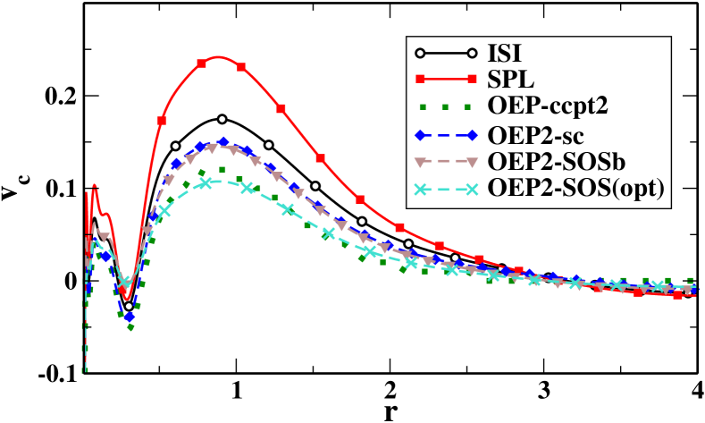
Figure 5: Correlation potentials obtained with different correlated OEP methods and two ACMs (ISI, SPL) for the neon atom.

As a further example we consider the case of the beryllium atom which is known to be a rather extreme case where the GL2 potential performs poorly, overestimating the correct correlation potential, such that self-consistent OEP-GL2 calculations fail to converge. Thus, in Fig. 6 we report the various correlation potentials computed for beryllium (note that in the bottom panel we report also the accurate second-order OEP potentials for comparison). Inspection of the plots shows that also in this difficult case the ACMs potentials, especially ISI and revISI, improve substantially over GL2 being comparable to the OEP2-SOSb and OEP2-SOS(opt) approaches. Note also that the accurate OEP2-sc method instead yields an underestimation of the correlation potential of the beryllium atom.

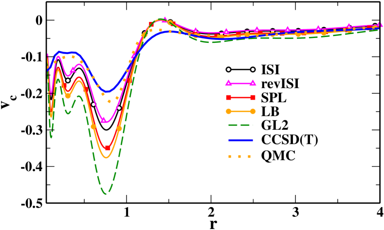
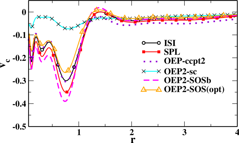
Figure 6: Correlation potentials obtained with different methods for the beryllium atom.

The analysis discussed above, evidenced the similarity of the ACMs potentials with scaled GL2 ones ^{53, 54, 55}. This finding is not completely surprising if we inspect the magnitudes of the different contributions forming the ACM potential in Eq. (2), i.e. $D^{\rm ACM}_{E_{x}}$, $D^{\rm ACM}_{E_{c}^{\rm GL2}}$, $D^{\rm ACM}_{W_{\infty}}$, and $D^{\rm ACM}_{W^{\prime}_{\infty}}$ (see Table 3).

Table 3: Values of the partial derivatives appearing in Eq. (2) for the various ACM correlation functionals of different atoms.

		$D^{\rm ACM}_{E_{x}}-1$	$D^{\rm ACM}_{E_{c}^{\rm GL2}}$	$D^{\rm ACM}_{W_{\infty}}$	$D^{\rm ACM}_{W^{\prime}_{\infty}}$
He	ISI	-0.029	0.642	0.029	0.006
	revISI	-0.036	0.615	0.036	0.009
	SPL	-0.014	0.699	0.014	-
	LB	-0.012	0.757	0.012	-
Be	ISI	-0.030	0.617	0.030	0.005
	revISI	-0.038	0.570	0.038	0.007
	SPL	-0.011	0.726	0.011	-
	LB	-0.009	0.782	0.009	-
Ne	ISI	-0.014	0.724	0.014	0.002
	revISI	-0.018	0.683	0.018	0.003
	SPL	-0.005	0.819	0.005	-
	LB	-0.004	0.869	0.004	-
Ar	ISI	-0.007	0.079	0.007	0.001
	revISI	-0.010	0.751	0.010	0.001
	SPL	-0.002	0.873	0.002	-
	LB	-0.002	0.904	0.002	-

The data show in fact that the main contribution to the potential of any of the ACMs is a scaled GL2 component, with a magnitude of about 70%. This finding traces back to the fact that the ACMs are effectively all-order renormalizations of the density functional perturbation theory ¹⁵, thus they basically perform a “rescaling” of the GL2 correlation contribution. This feature puts these potentials not only in relation with the spin-opposite-scaled OEP methods (OEP2-SOS), as mentioned above, but also with the recently developed self-consistent OEP double-hybrid ⁷ method, which also shows a similar signature. Then, the success of the later methods in self-consistent calculations can be considered as promising indicator for the quality of the ACM potentials and the possible success of future self-consistent calculations based on the ACM functionals.

We remark anyway that, despite the scaled GL2 is the main component of the correlation potential of ACMs, other contributions may also be present with a non negligible effect. This can be seen, for example, in Fig. 7 where we plot the quantity $v_{c}^{\rm ACM}-D^{\rm ACM}_{E_{c}^{\rm GL2}}v_{c}^{\rm GL2}$ for the Ne atom.

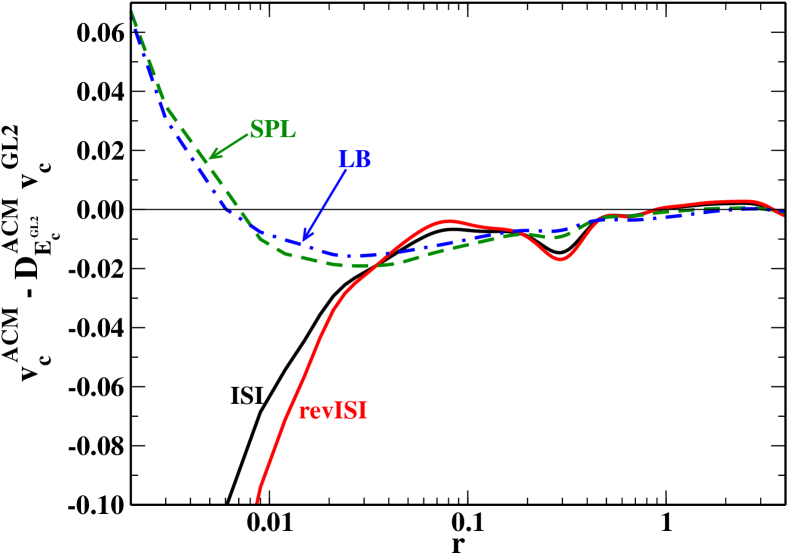
Figure 7: Difference between the correlation potentials of various adiabatic connection models and the scaled second-order Görling Levy correlation potential ($v_{c}^{\rm ACM}-D^{\rm ACM}_{E_{c}^{\rm GL2}}v_{c}^{\rm GL2}$) for the neon atom.

The plot shows that all the ACM potentials show relevant features in the core regions (i.e. $v_{c}^{\rm ACM}-D^{\rm ACM}_{E_{c}^{\rm GL2}}v_{c}^{\rm GL2}\neq 0$), that possibly originate from the larger correlation effects felt by core electrons, implying a larger contribution from the $D^{\rm ACM}_{W_{\infty}}$ component (see also the subsection Potentials for the strong-interaction limit). This is more evident for ISI and revISI, whereas, the SPL and LB correlation potentials are slightly closer to scaled GL2 potentials.

It is worth to note also that the “renormalization” effect of the ACM correlation potentials will increase when systems with stronger correlation are considered. Unfortunately, for such systems the OEP equation needed to generate the GL2 potential cannot be generally solved; thus we had to limit our investigation only to the simple case of the F^- anion, to be compared with the Ne atom. This comparison is shown in Fig. 8 for the case of the revISI correlation potential (other ACMs behave similarly).

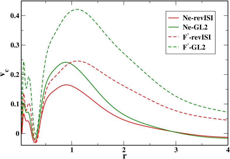
Figure 8: GL2 and revISI correlation potentials for the Ne atom and the F^- anion.

From the plot it can be seen that for the F^- anion, where correlation effects are slightly larger than in Ne, indeed a greater difference between the revISI and the GL2 potentials is found. This fact is also confirmed by the computed value of $D^{\rm ACM}_{E_{c}^{\rm GL2}}$ that for F^- is 0.583 (to be compared with 0.683 in Ne, see Table 3); note also that $D^{\rm ACM}_{W_{\infty}}$ is 0.030 for F^- while it is 0.018 for the neon atom.

To conclude, in Fig. 9 we report the correlation potentials computed for two simple molecules, namely H₂ and N₂.

Figure 9: Correlation potentials of different adiabatic connection models as well of the second order Görling-Levy (GL2) correlation for the H₂ (top) and N₂ (bottom) molecules, plotted along the bond axis. The vertical lines indicate the positions of the atoms in each molecule.

In these cases we have also used as a reference the correlated potential obtained from relaxed CCSD(T) density observing the same qualitative behavior as already found in atoms. Thus, all the ACMs provide a reduction of the correlation potential with respect to GL2. In particular, ISI and revISI provide a slight larger reduction than SPL and LB.

Figure 10: Correlation potentials for nitrogen dimer obtained with several correlated OEP methods and two ACMs (ISI, SPL).

Also here the direct comparison with several correlated OEP potentials made for nitrogen dimer reveals remarkably good performance for all ACMs. The ISI and SPL give almost the same potentials as OEP2-sc which is considered as the state-of-the-art correlated OEP method.

4 Conclusions

We have studied the correlation potentials produced by different adiabatic connection models to investigate whether these methods are able to produce, besides reasonable energies ^{31, 32, 33}, also physically meaningful potentials. This is, in fact, a fundamental issue in view of a possible future use of the ACMs in self-consistent calculations.

Our results showed that indeed all the investigated functionals are able to provide rather accurate correlation potentials, with ISI and revISI being slightly superior to SPL and LB. In particular, all the considered correlation potentials display the correct features of the exact correlation potential and reduce the overestimation behavior which is typical of the GL2 method ^{8, 76}. Thus, all in all, the ACM-based correlation potentials are comparable to those produced by some state-of-the-art optimized effective potential methods (OEP2-sc ^{8, 10}, OEP2-SOS ^{54, 55}).

These results suggest that it might be worth to pursue the realization of self-consistent calculations using the ACM XC functionals, which would provide a final assessment of their quality. However, to reach this goal a few issues need first to be solved. In particular, one needs to develop proper density functionals for the $\lambda\to\infty$ limit, in order to replace the gradient expansions of Eqs. (5) and (6), which lead to divergences in the potential. The functionals of Refs. ^{25, 26, 27} are already very good candidate, although they pose new technical problems at the implementation level due to their non-local density dependence. If one wants to stay within gradient approximations, then the PC GEA should be renormalized into GGA’s. Moreover, a proper OEP scheme, similar to the one used for the implementation of self-consistent double hybrids ⁷, need to be implemented to deal with the various terms appearing in Eq. (2), which are both of implicit non-local and explicit semilocal types.

5 Acknowledgements

S.Ś is grateful to the Polish National Science Center for the partial financial support under Grant No. 2016/21/D/ST4/00903. P.G.-G. and S.G. acknowledge funding from the European Research Council under H2020/ERC Consolidator Grant corr-DFT (Grant Number 648932), and T.J.D. is grateful to the Vrije Universiteit Amsterdam for a University Research Fellowship.

Appendix A Adiabatic connection models

In this work we consider several ACMs. They main features of each one are described below.

ISI functional ¹⁵. The XC energy is

$$E_{xc}^{\rm ISI}=W_{\infty}+\frac{2X}{Y}\left[\sqrt{1+Y}-1-Z\ln\left(\frac{\sqrt{1+Y}+Z}{1+Z}\right)\right]\ ,$$ (17)

with

$$X=\frac{xy^{2}}{z^{2}}\;,\;Y=\frac{x^{2}y^{2}}{z^{4}}\;,\;Z=\frac{xy^{3}}{z^{3}}-1\;,$$ (18)

$$x=-4E_{c}^{\rm GL2}\;,\;y=W^{\prime}_{\infty}\;,\;z=E_{x}-W_{\infty}.$$ (19)

revISI functional ¹⁹. The XC energy is

$$E_{xc}^{\rm revISI}=W_{\infty}+\frac{b}{\sqrt{1+c}+d}\ ,$$ (20)

with

$$b = -\frac{8E_{c}^{\rm GL2}(W^{\prime}_{\infty})^{2}}{(E_{x}-W_{\infty})^{2}}\ ,$$ (21)

$$c = \frac{16(E_{c}^{\rm GL2}W^{\prime}_{\infty})^{2}}{(E_{x}-W_{\infty})^{4}}\ ,$$ (22)

$$d = -1-\frac{8E_{c}^{\rm GL2}(W^{\prime}_{\infty})^{2}}{(E_{x}-W_{\infty})^{3}}\ .$$ (23)

SPL functional ¹⁷. The XC energy is

$$E_{xc}^{\rm SPL}=E_{x}+(E_{x}-W_{\infty})\left[\frac{\sqrt{1+2\chi}-1-\chi}{\chi}\right]\ ,$$ (24)

with

$$\chi=\frac{2E_{c}^{\rm GL2}}{W_{\infty}-E_{x}}\ .$$ (25)

LB functional ²⁹. The XC energy is

$$E_{xc}^{\rm LB}=E_{x}+\frac{2b}{c}\left[\sqrt{1+c}-\frac{1+c/2}{1+c}-c\right]\ ,$$ (26)

with

$$b=\frac{E_{x}-W_{\infty}}{2}\;,\;c=\frac{8E_{c}^{\rm GL2}}{5(W_{\infty}-E_{x})}\ .$$ (27)

Appendix B Functional derivative of the PC functionals

The functional derivative of Eqs. (5) and (6) with respect to the density is

$$\frac{\delta{W}^{\rm PC}_{\infty}[\rho]}{\delta\rho(\mathbf{r})}=\frac{4A}{3}\rho(\mathbf{r})^{1/3}-2B\frac{\nabla^{2}\rho(\mathbf{r})}{\rho(\mathbf{r})^{4/3}}+\frac{4B}{3}\frac{|\nabla\rho(\mathbf{r})|^{2}}{\rho(\mathbf{r})^{7/3}},$$ (28)

$$\frac{\delta{W}^{\prime\rm PC}_{\infty}[\rho]}{\delta\rho(\mathbf{r})}=\frac{3C}{2}\rho(\mathbf{r})^{1/2}-2D\frac{\nabla^{2}\rho(\mathbf{r})}{\rho(\mathbf{r})^{7/6}}+\frac{7D}{6}\frac{|\nabla\rho(\mathbf{r})|^{2}}{\rho(\mathbf{r})^{13/6}}.$$ (29)

In order to study which terms are responsible for the divergence observed (see the subsection Potentials for the strong-interaction limit), we consider the asymptotic expression ⁷⁷ for a density of $N$ electrons bound by a total positive charge $Z$, with $r=|\mathbf{r}|$,

$$\rho(r\rightarrow\infty)\sim r^{\beta}e^{-{\alpha}r},$$ (30)

with $\alpha=2\sqrt{2I}$, $\beta=\frac{Z-N+1}{\sqrt{2I}}-1$, and $I$ the first ionization potential (e.g. for the Ne atom $\alpha\approx 2.5$ and $\beta\approx-0.2$). By plugging Eq. (30) into Eq. (28), one sees that the second and third terms go to leading order like $r^{-\frac{\beta}{3}}e^{\frac{\alpha}{3}r}$; however the second term is multiplied by a negative constant, namely $-2B$, which determines the divergence to $-\infty$ over the third term, whose prefactor is $\frac{4B}{3}$. Analogously, for Eq. (29), one sees that the second and third terms, again, diverge with same leading order, which, in this case, is $r^{-\frac{\beta}{6}}e^{\frac{\alpha}{6}r}$. In this latter case, however, the second term is multiplied by the positive constant $-2D$, which determines the divergence to $+\infty$ over the third term, whose prefactor is $\frac{7D}{6}$. Since all the ACM potentials calculated in this work make use of the PC approximation for the strong-interaction limit terms, they all show a negative divergence, appearing ‘earlier’ in the SPL and LB than in the ISI and revISI models (as these latter also include the ingredient $\frac{\delta{W}^{\prime\rm PC}_{\infty}[\rho]}{\delta\rho(\mathbf{r})}$, which partially compensates the asymptotically dominant term). Moreover, while this analysis applies to the exact asymptotic density behavior, the use of gaussian basis sets worsens the divergence at large $r$.

References

- Scuseria and Staroverov 2005 Scuseria, G. E.; Staroverov, V. N. In Theory and Applications of Computational Chemistry: The First Forty Years; Dykstra, C. E., Frenking, G., Kim, K. S., Scuseria, G. E., Eds.; Elsevier, Amsterdam, 2005
- Della Sala et al. 2016 Della Sala, F.; Fabiano, E.; Constantin, L. A. Kinetic-energy-density dependent semilocal exchange-correlation functionals. Int. J. Quantum Chem. 2016, 116, 1641–1694
- Perdew and Schmidt 2001 Perdew, J. P.; Schmidt, K. Jacob’s ladder of density functional approximations for the exchange-correlation energy. AIP Conference Proceedings 2001, 577, 1–20
- Jiang and Engel 2007 Jiang, H.; Engel, E. Random-phase-approximation-based correlation energy functionals: Benchmark results for atoms. J. Chem. Phys. 2007, 127, 184108
- Chen et al. 2017 Chen, G. P.; Voora, V. K.; Agee, M. M.; Balasubramani, S. G.; Furche, F. Random-Phase Approximation Methods. Ann. Rev. Phys. Chem. 2017, 68, 421–445
- Grimme 2006 Grimme, S. Semiempirical hybrid density functional with perturbative second-order correlation. J. Chem. Phys. 2006, 124, 034108
- Śmiga et al. 2016 Śmiga, S.; Franck, O.; Mussard, B.; Buksztel, A.; Grabowski, I.; Luppi, E.; Toulouse, J. Self-consistent double-hybrid density-functional theory using the optimized-effective-potential method. J. Chem. Phys. 2016, 145, 144102
- Bartlett et al. 2005 Bartlett, R. J.; Grabowski, I.; Hirata, S.; Ivanov, S. The exchange-correlation potential in ab initio density functional theory. J. Chem. Phys. 2005, 122, 034104
- Bartlett et al. 2005 Bartlett, R. J.; Lotrich, V. F.; Schweigert, I. V. Ab initio density functional theory: The best of both worlds? J. Chem. Phys. 2005, 123, 062205
- Grabowski et al. 2007 Grabowski, I.; Lotrich, V.; Bartlett, R. J. Ab initio density functional theory applied to quasidegenerate problems. J. Chem. Phys. 2007, 127, 154111
- Harris and Jones 1974 Harris, J.; Jones, R. O. The surface energy of a bounded electron gas. J. Phys. F: Metal Physics 1974, 4, 1170
- Langreth and Perdew 1975 Langreth, D.; Perdew, J. P. The exchange-correlation energy of a metallic surface. Solid State Commun. 1975, 17, 1425 – 1429
- Gunnarsson and Lundqvist 1976 Gunnarsson, O.; Lundqvist, B. I. Exchange and correlation in atoms, molecules, and solids by the spin-density-functional formalism. Phys. Rev. B 1976, 13, 4274–4298
- Savin et al. 2003 Savin, A.; Colonna, F.; Pollet, R. Adiabatic connection approach to density functional theory of electronic systems. Int. J. Quantum Chem. 2003, 93, 166–190
- Seidl et al. 2000 Seidl, M.; Perdew, J. P.; Kurth, S. Simulation of All-Order Density-Functional Perturbation Theory, Using the Second Order and the Strong-Correlation Limit. Phys. Rev. Lett. 2000, 84, 5070–5073
- Görling and Levy 1994 Görling, A.; Levy, M. Exact Kohn-Sham scheme based on perturbation theory. Phys. Rev. A 1994, 50, 196–204
- Seidl et al. 1999 Seidl, M.; Perdew, J. P.; Levy, M. Strictly correlated electrons in density-functional theory. Phys. Rev. A 1999, 59, 51
- Seidl et al. 2007 Seidl, M.; Gori-Giorgi, P.; Savin, A. Strictly correlated electrons in density-functional theory: A general formulation with applications to spherical densities. Phys. Rev. A 2007, 75, 042511
- Gori-Giorgi et al. 2009 Gori-Giorgi, P.; Vignale, G.; Seidl, M. Electronic Zero-Point Oscillations in the Strong-Interaction Limit of Density Functional Theory. J. Chem. Theory Comput. 2009, 5, 743–753
- Malet et al. 2013 Malet, F.; Mirtschink, A.; Cremon, J. C.; Reimann, S. M.; Gori-Giorgi, P. Kohn-Sham density functional theory for quantum wires in arbitrary correlation regimes. Phys. Rev. B 2013, 87, 115146
- Lewin 2017 Lewin, M. Semi-classical limit of the Levy-Lieb functional in Density Functional Theory. arXiv:1706.02199 2017
- Cotar et al. 2017 Cotar, C.; Friesecke, G.; Klüppelberg, C. Smoothing of transport plans with fixed marginals and rigorous semiclassical limit of the Hohenberg-Kohn functional. arXiv:1706.05676 2017
- Grossi et al. 2017 Grossi, J.; Kooi, D. P.; Giesbertz, K. J. H.; Seidl, M.; Cohen, A. J.; Mori-Sánchez, P.; Gori-Giorgi, P. Fermionic Statistics in the Strongly Correlated Limit of Density Functional Theory. J. Chem. Theory Comput. 2017, 13, 6089–6100
- Seidl et al. 2000 Seidl, M.; Perdew, J. P.; Kurth, S. Density functionals for the strong-interaction limit. Phys. Rev. A 2000, 62, 012502
- Wagner and Gori-Giorgi 2014 Wagner, L. O.; Gori-Giorgi, P. Electron avoidance: A nonlocal radius for strong correlation. Phys. Rev. A 2014, 90, 052512
- Bahmann et al. 2016 Bahmann, H.; Zhou, Y.; Ernzerhof, M. The shell model for the exchange-correlation hole in the strong-correlation limit. J. Chem. Phys 2016, 145, 124104
- Vuckovic and Gori-Giorgi 2017 Vuckovic, S.; Gori-Giorgi, P. Simple Fully Nonlocal Density Functionals for Electronic Repulsion Energy. J. Phys. Chem. Lett. 2017, 8, 2799–2805
- Seidl et al. 2005 Seidl, M.; Perdew, J. P.; Kurth, S. Erratum: Density functionals for the strong-interaction limit [Phys. Rev. A 62, 012502 (2000)] Phys. Rev. A 2005, 72, 029904
- Liu and Burke 2009 Liu, Z.-F.; Burke, K. Adiabatic connection in the low-density limit. Phys. Rev. A 2009, 79, 064503
- Ernzerhof 1996 Ernzerhof, M. Construction of the adiabatic connection. Chem. Phys. Lett. 1996, 263, 499 – 506
- Fabiano et al. 2016 Fabiano, E.; Gori-Giorgi, P.; Seidl, M.; Della Sala, F. Interaction-Strength Interpolation Method for Main-Group Chemistry: Benchmarking, Limitations, and Perspectives. J. Chem. Theory Comput. 2016, 12, 4885–4896
- Giarrusso et al. 2018 Giarrusso, S.; Gori-Giorgi, P.; Della Sala, F.; Fabiano, E. Assessment of interaction-strength interpolation formulas for gold and silver clusters. J. Chem. Phys. 2018, 148, 134106
- Vuckovic et al. 2018 Vuckovic, S.; Gori-Giorgi, P.; Della Sala, F.; Fabiano, E. Restoring Size Consistency of Approximate Functionals Constructed from the Adiabatic Connection. J. Phys. Chem. Lett. 2018, 9, 3137
- Jankowski et al. 2005 Jankowski, K.; Grabowski, I.; Nowakowski, K.; Wasilewski, J. Ab initio Correlation Effects in Density Functional Theories: An Electron-Distribution-Based Study for Neon. Collection of Czechoslovak Chemical Communications 2005, 70, 1157–1176
- Fabiano and Della Sala 2007 Fabiano, E.; Della Sala, F. Localized exchange-correlation potential from second-order self-energy for accurate Kohn-Sham energy gap. J. Chem. Phys 2007, 126, 214102
- Grabowski et al. 2011 Grabowski, I.; Teale, A. M.; Śmiga, S.; Bartlett, R. J. Comparing ab initio density-functional and wave function theories: The impact of correlation on the electronic density and the role of the correlation potential. J. Chem. Phys. 2011, 135, 114111
- Grabowski et al. 2014 Grabowski, I.; Teale, A. M.; Fabiano, E.; Śmiga, S.; Buksztel, A.; Della Sala, F. A density difference based analysis of orbital-dependent exchange-correlation functionals. Mol. Phys. 2014, 112, 700–710
- Buijse et al. 1989 Buijse, M. A.; Baerends, E. J.; Snijders, J. G. Analysis of correlation in terms of exact local potentials: Applications to two-electron systems. Phys. Rev. A 1989, 40, 4190–4202
- Umrigar and Gonze 1994 Umrigar, C. J.; Gonze, X. Accurate exchange-correlation potentials and total-energy components for the helium isoelectronic series. Phys. Rev. A 1994, 50, 3827 –3837
- Gritsenko et al. 1994 Gritsenko, O.; van Leeuwen, R.; Baerends, E. J. Analysis of electron interaction and atomic shell structure in terms of local potentials. J. Chem. Phys. 1994, 101, 8955
- Filippi et al. 1996 Filippi, C.; Gonze, X.; Umrigar, C. J. In Recent developments and applications in modern DFT; Seminario, J. M., Ed.; Elsevier: Amsterdam, 1996; pp 295–321
- Baerends and Gritsenko 1996 Baerends, E. J.; Gritsenko, O. V. Effect of molecular dissociation on the exchange-correlation Kohn-Sham potential. Phys. Rev. A 1996, 54, 1957–1972
- Gritsenko et al. 1996 Gritsenko, O. V.; van Leeuwen, R.; Baerends, E. J. Molecular exchange-correlation Kohn-Sham potential and energy density from ab initio first- and second-order density matrices: Examples for XH (X= Li, B, F). J. Chem. Phys. 1996, 104, 8535
- Tempel et al. 2009 Tempel, D. G.; Martínez, T. J.; Maitra, N. T. Revisiting Molecular Dissociation in Density Functional Theory: A Simple Model. J. Chem. Theory. Comput. 2009, 5, 770–780
- Helbig et al. 2009 Helbig, N.; Tokatly, I. V.; Rubio, A. Exact Kohn-Sham potential of strongly correlated finite systems. J. Chem. Phys. 2009, 131, 224105
- Ryabinkin et al. 2015 Ryabinkin, I. G.; Kohut, S. V.; Staroverov, V. N. Reduction of electronic wave functions to Kohn-Sham effective potentials. Phys. Rev. Lett. 2015, 115, 083001
- Ospadov et al. 2017 Ospadov, E.; Ryabinkin, I. G.; Staroverov, V. N. Improved method for generating exchange-correlation potentials from electronic wave functions. J. Chem. Phys. 2017, 146, 084103
- Kohut et al. 2016 Kohut, S. V.; Polgar, A. M.; Staroverov, V. N. Origin of the step structure of molecular exchange–correlation potentials. Phys. Chem. Chem. Phys. 2016, 18, 20938–20944
- Hodgson et al. 2016 Hodgson, M. J. P.; Ramsden, J. D.; Godby, R. W. Origin of static and dynamic steps in exact Kohn-Sham potentials. Phys. Rev. B 2016, 93, 155146
- Ying et al. 2016 Ying, Z. J.; Brosco, V.; Lopez, G. M.; Varsano, D.; Gori-Giorgi, P.; Lorenzana, J. Anomalous scaling and breakdown of conventional density functional theory methods for the description of Mott phenomena and stretched bondsPhys. Rev. B 2016, 94, 075154
- Benítez and Proetto 2016 Benítez, A.; Proetto, C. R. Kohn-Sham potential for a strongly correlated finite system with fractional occupancy. Phys. Rev. A 2016, 94, 052506
- Ryabinkin et al. 2017 Ryabinkin, I. G.; Ospadov, E.; Staroverov, V. N. Exact exchange-correlation potentials of singlet two-electron systems. J. Chem. Phys. 2017, 147, 164117
- Grabowski et al. 2013 Grabowski, I.; Fabiano, E.; Della Sala, F. Optimized effective potential method based on spin-resolved components of the second-order correlation energy in density functional theory. Phys. Rev. B 2013, 87, 075103
- Grabowski et al. 2014 Grabowski, I.; Fabiano, E.; Teale, A. M.; Śmiga, S.; Buksztel, A.; Della Sala, F. Orbital-dependent second-order scaled-opposite-spin correlation functionals in the optimized effective potential method. J. Chem. Phys 2014, 141, 024113
- Śmiga et al. 2016 Śmiga, S.; Della Sala, F.; Buksztel, A.; Grabowski, I.; Fabiano, E. Accurate Kohn–Sham ionization potentials from scaled‐opposite‐spin second‐order optimized effective potential methods. J. Comput. Chem. 2016, 37, 2081–2090
- Medvedev et al. 2017 Medvedev, M. G.; Bushmarinov, I. S.; Sun, J.; Perdew, J. P.; Lyssenko, K. A. Density functional theory is straying from the path toward the exact functional. Science 2017, 355, 49–52
- Brorsen et al. 2017 Brorsen, K. R.; Yang, Y.; Pak, M. V.; Hammes-Schiffer, S. Is the Accuracy of Density Functional Theory for Atomization Energies and Densities in Bonding Regions Correlated? J. Phys. Chem. Lett. 2017, 8, 2076–2081
- Korth 2017 Korth, M. Density Functional Theory: Not Quite the Right Answer for the Right Reason Yet. Angew. Chem. Int. Ed. 2017, 56, 5396–5398
- Mezei et al. 2017 Mezei, P. D.; Csonka, G. I.; Kállay, M. Electron Density Errors and Density-Driven Exchange-Correlation Energy Errors in Approximate Density Functional Calculations. J. Chem. Theory Comput. 2017, 13, 4753–4764
- Della Sala et al. 2015 Della Sala, F.; Fabiano, E.; Constantin, L. A. Kohn-Sham kinetic energy density in the nuclear and asymptotic regions: Deviations from the von Weizsäcker behavior and applications to density functionals. Phys. Rev. B 2015, 91, 035126
- Constantin et al. 2016 Constantin, L. A.; Fabiano, E.; Pitarke, J. M.; Della Sala, F. Semilocal density functional theory with correct surface asymptotics. Phys. Rev. B 2016, 93, 115127
- Malet and Gori-Giorgi 2012 Malet, F.; Gori-Giorgi, P. Strong Correlation in Kohn-Sham Density Functional Theory. Phys. Rev. Lett. 2012, 109, 246402
- Mendl et al. 2014 Mendl, C. B.; Malet, F.; Gori-Giorgi, P. Wigner localization in quantum dots from Kohn-Sham density functional theory without symmetry breaking. Phys. Rev. B 2014, 89, 125106
- Grabowski and Lotrich 2005 Grabowski, I.; Lotrich, V. Accurate orbital-dependent correlation and exchange-correlation potentials from non-iterative ab initio dft calculations. Mol. Phys. 2005, 103, 2085–2092
- Görling 2005 Görling, A. Orbital- and state-dependent functionals in density-functional theory. J. Chem. Phys. 2005, 123, 062203
- Stanton et al. 2007 Stanton, J. F. et al. ACES II; Quantum Theory Project: Gainesville, Florida, 2007
- Dunning Jr. 1989 Dunning Jr., T. H. Gaussian basis sets for use in correlated molecular calculations. I. The atoms boron through neon and hydrogen. J. Chem. Phys 1989, 90, 1007–1023
- Grabowski et al. 2002 Grabowski, I.; Hirata, S.; Ivanov, S.; Bartlett, R. J. Ab initio density functional theory: OEP-MBPT(2). A new orbital-dependent correlation functional. J. Chem. Phys. 2002, 116, 4415–4425
- Widmark et al. 1990 Widmark, P.-O.; Malmqvist, P.-Å.; Roos, B. O. Density matrix averaged atomic natural orbital (ANO) basis sets for correlated molecular wave functions. Theoretica chimica acta 1990, 77, 291–306
- Peterson and Dunning Jr. 2002 Peterson, K. A.; Dunning Jr., T. H. Accurate correlation consistent basis sets for molecular core–valence correlation effects: The second row atoms Al–Ar, and the first row atoms B–Ne revisited. J. Chem. Phys 2002, 117, 10548–10560
- Seidl et al. 2017 Seidl, M.; Di Marino, S.; Gerolin, A.; Nenna, L.; Giesbertz, K. J. H.; Gori-Giorgi, P. The strictly-correlated electron functional for spherically symmetric systems revisited. arXiv:1702.05022 [cond-mat.str-el] 2017
- Wu and Yang 2003 Wu, Q.; Yang, W. A direct optimization method for calculating density functionals and exchange–correlation potentials from electron densities. J. Chem. Phys. 2003, 118, 2498
- Umrigar and Gonze 1994 Umrigar, C. J.; Gonze, X. Accurate exchange-correlation potentials and total-energy components for the helium isoelectronic series. Phys. Rev. A 1994, 50, 3827
- Filippi et al. 1996 Filippi, C.; Umrigar, C. J.; Gonze, X. Separation of the exchange-correlation potential into exchange plus correlation: An optimized effective potential approach. Phys. Rev. A 1996, 54, 4810
- Kodera et al. 2018 Kodera, M.; Miyasita, M.; Shimizu, H.; Higuchi, K.; Higuchi, M. Renormalized Møller–Plesset Correlation Energy Functional Used in the Optimized Effective Potential Method. J. Phys. Soc. Jpn. 2018, 87, 014302
- Schweigert et al. 2006 Schweigert, I. V.; Lotrich, V. F.; Bartlett, R. J. Ab initio correlation functionals from second-order perturbation theory. J. Chem. Phys. 2006, 125, 104108
- Katriel and Davidson 1980 Katriel, J.; Davidson, E. R. Asymptotic behavior of atomic and molecular wave functions. Proc. Natl. Acad. Sci. USA 1980, 77, 4403–4406