Properties of structure functions from helicity components
of light quarks and antiquarks in the statistical model

Abstract

In the quantum statistical parton distributions approach proposed more than one decade ago to describe the parton structure, new properties are now understood, in particular, the relation between quarks and antiquarks which leads to very specific properties. The simultaneous treatment of unpolarized and polarized Parton Distribution Functions (PDFs) allows a determination of thermodynamical potentials (the master parameters of the model) which drive their behavior and as a consequence those of the structure functions. The existence of a possible relation between the gluon and a $q~{}\bar{q}$ pair leads to define a toy model for the unpolarized and polarized gluon. In view of forthcoming experimental results in the large $x$ region specific predictions made by the model are presented.

I Introduction

Our main objective is to build quarks structure where constitutive elements can be understood through their parameters which are easily associated with the quark properties. The first point to clarify is the choice of a statistical model. Taking the example of a proton at rest which contains three quarks a statistical treatment seems not justified due to the low number of elements. However, when a proton is accelerated in a collider the energy increase has not only an effect on the masses but also to create a large number of $q~{}\bar{q}$ pairs or a quark gluon plasma where in a p-p collison materializes mainly in primary unstable particles observed in a detector by a large number of tracks. The production of numerous pairs and gluons provide a justification for a statistical treatment of the partons interaction process. Moreover, the fact that a quark is described in our model by a Fermi function means that it is already dressed to live in a surrounding nuclear medium made of quarks.

The statistical approach is characterized by thermodynamical potentials whose values are the master parameters, they drive not only the shape of the PDFs but are found to control some specific properties of the structure functions. In order to introduce the maximum constraints one decides to work from the beginning with helicity components which are the building blocks of both the polarized and unpolarized PDFs a unique situation in the domain. It is clear that the number of polarized data is much smaller than the unpolarized ones and also that they are limited to a medium energy region, however the RHIC experiments enlarge somehow this domain but a large gap remains to reach the LHC energy.

The objective of the paper is to discuss the consequence of the statistical approach on the quarks structure because from a collection of results obtained through the years one gets now a better global view.

In section 2, a review of the basic elements of the quarks distribution is presented together with the notations. In section 3, a proof is given to show how the antiquarks PDFs can be deduced from the quarks by using different constraints in the fitting process. Section 4 is devoted to analyze the different helicity components and how their effect is put in evidence in structure functions. In section 5, a toy model is introduced to define new unpolarized and polarized gluon PDFs, which is inspired by the relation between gluons and $q\bar{q}$ pairs. The conclusions are presented in section 6.

II Basic elements of the quark distributions

The PDFs are the essential elements to evaluate scattering processes in QCD. In the absence of a theory they are usually parametrized with polynomials Refs ct14 ; mmht14 , to go beyond this approximation and in an attempt to define a more physical structure for the quarks a statistical approach was proposed many years ago to build up the PDFs bbs1 .

Let us now describe the main features of the statistical approach. The fermion distributions are given by the sum of two terms, a quasi Fermi-Dirac function of helicity $h=\pm$ and a helicity independent diffractive contribution:

$$xq^{h}(x,Q^{2}_{0})=\frac{A_{q}X^{h}_{q}x^{b_{q}}}{\exp[(x-X^{h}_{q})/\bar{x}]+1}+\frac{\tilde{A}_{q}x^{\tilde{b}_{q}}}{\exp(x/\bar{x})+1}~{},$$ (1)

for the quarks and for the antiquarks the ansatz:

$$x\bar{q}^{h}(x,Q^{2}_{0})=\frac{{\bar{A}_{q}}(X^{-h}_{0q})^{-1}x^{\bar{b}_{q}}}{\exp[(x+X^{-h}_{0q})/\bar{x}]+1}+\frac{\tilde{A}_{q}x^{\tilde{b}_{q}}}{\exp(x/\bar{x})+1}~{},$$ (2)

at the input energy scale $Q_{0}^{2}=1\mbox{GeV}^{2}$.

With the above definitions the diffractive term is the same for flavor $u,d$, but has a specific expression for other flavors. It is absent in the quark helicity distribution $\Delta q=q^{+}-q^{-}$, the quark valence contribution $q-\bar{q}$ and the difference $u-d$.
In the numerator of the non-diffractive parts of Eq. (1) the multiplicative factor $X^{h}_{q}$ allows to separate $u$ and $d$ quarks since one assumes $A_{u}=A_{d}$, the term $x^{b_{q}}$ imply a modification of the quantum statistical form, this term is introduced in order to control the small $x$ behaviour. The parameter $\bar{x}=0.09$ plays the role of a universal temperature and $X^{\pm}_{q}$ are the two thermodynamical potentials of a quark $q$, with helicity $h=\pm$. They represent the fundamental parameters of the model because they drive the PDFs behaviour. For convenience the values of the potentials obtained in BS15 Bourrely:2015kla are recalled:

$$X_{u}^{+}=0.475\pm 0.001,~{}X_{u}^{-}=0.307\pm 0.001,$$

$$X_{d}^{+}=0.245\pm 0.001,~{}X_{d}^{-}=0.309\pm 0.001,$$

$$X_{s}^{+}=0.011\pm 0.001,~{}X_{s}^{-}=0.015\pm 0.001.$$ (3)

III Generation of the antiquarks distribution

To adopt a coherent scheme it is natural to suppose that antiquarks must also contain a Fermi part analogous to the quarks and also in addition a diffractive part being the same as in the quarks, all these constraints lead to a general expression like:

$$x\bar{q}^{h}(x,Q^{2}_{0})=\frac{\bar{A}_{q}^{{}^{\prime}h}x^{\bar{b}_{q}}}{\exp[(x-Y^{h}_{q})/\bar{x}]+1}+\frac{\tilde{A}_{q}x^{\tilde{b}_{q}}}{\exp(x/\bar{x})+1}~{}.$$ (4)

This distribution depend on the new parameters $\bar{A}_{q}^{{}^{\prime}h},Y^{h}_{q}$ compared to Eq. (2). In order to determine these parameters in a fitting process the constraint of the valence sum rule is added

$$\int(q(x)-\bar{q}(x))dx=N_{q},\quad\mbox{where}\quad N_{q}=2,1\quad\mbox{for~{}~{} u, d}\,,$$ (5)

(this sum rule is independent of the diffractive part) and a second constraint which comes from the momentum sum rule

$$\int\sum_{i}[xq_{i}(x)+x\bar{q}_{i}(x))+xG(x)]dx=1\,,$$ (6)

where $G(x)$ is the unpolarized gluon distribution. Making a fit at NLO of unpolarized and polarized experimental data analogous to the one discussed in BS15 Ref. Bourrely:2015kla one finds for the potentials a solution:

$$Y_{u}^{-}=-0.475,\quad\quad Y_{u}^{+}=-0.307$$

$$Y_{d}^{-}=-0.244,\quad\quad Y_{d}^{+}=-0.309\,,$$ (7)

where a comparison with the solution obtained in BS15 (3) leads to

$$Y_{u}^{-}=-X_{u}^{+},\quad Y_{u}^{+}=-X_{u}^{-},\quad Y_{d}^{-}=-X_{d}^{+},\quad Y_{d}^{+}=-X_{d}^{-}\,,$$ (8)

the change of sign in the $\bar{q}$ potentials and in the helicity find its origin from the unpolarized gluon whose potential is null $X_{q}^{\pm}+Y_{q}^{\mp}=0$, this point will be examined later.
The other parameters are given by:

$$A=1.943,\quad\quad b_{u}=b_{d}=0.471\quad\quad\bar{b}_{u}=\bar{b}_{d}=1.304,$$

$$\bar{A}_{u}^{{}^{\prime}+}=29.039,\quad\quad\bar{A}_{u}^{{}^{\prime}-}=18.768,$$

$$\bar{A}_{d}^{{}^{\prime}+}=28.851,\quad\quad\bar{A}_{d}^{{}^{\prime}-}=36.536,$$ (9)

By introducing the definition $\bar{A}^{{}^{\prime}h}_{q}=\bar{A}_{q}/X^{-h}_{q}$, the antiquarks distributions (4) become identical to Eq (2), where the four normalizations $\bar{A}^{{}^{\prime}h}_{q}$ are reduced to one constant $\bar{A}_{q}=8.915$. This result confirms the ansatz taken at the origin for the antiquarks, which was expected to be a solution of Eq. (4). To summarized an interesting relation between light quarks and antiquarks in the statistical approach was established with the objective to reduce the number of arbitrary distributions (see sec. V).

IV Properties of the unpolarized and polarized quark distributions

From the results obtained in Eq. (3) it is found for the light quarks the following hierarchy between the different potential components

$$X_{u}^{+}>X_{u}^{-}\simeq X_{d}^{-}>X_{d}^{+}.$$ (10)

In Eq. (7) the two potentials $X_{u}^{-},X_{d}^{-}$ have very close numerical values, which is a consequence of the near equality between $xu^{-}(x,Q^{2})$ and $xd^{-}(x,Q^{2})$.

It is easy to show that quarks helicity PDFs increase with the potentials value, while for antiquarks helicity PDFs increase when the potentials decrease.

As a consequence of the above hierarchy on potentials (10) it follows a hierarchy on the quarks helicity distributions,

$$xu_{+}(x)>xu_{-}(x)=xd_{-}(x)>xd_{+}(x)$$ (11)

and a obvious hierarchy for the antiquarks, namely

$$x\bar{d}_{-}(x)>x\bar{d}_{+}(x)=x\bar{u}_{+}(x)>x\bar{u}_{-}(x),$$ (12)

It is important to note that these inequalities Eqs. (11)-(12) are preserved by the NLO QCD evolution. An other remark is the fact that the initial analytic form Eqs. (1,2), is almost preserved by the $Q^{2}$ evolution with some small changes on the parameters numerical values. One clearly concludes that $u(x,Q^{2})>d(x,Q^{2})$ implies a flavor-asymmetric light sea, i.e. $\bar{d}(x,Q^{2})>\bar{u}(x,Q^{2})$, a trivial consequence of the Pauli exclusion principle, which is built in. Indeed this is based on the fact that the proton contains two $u$ quarks and only one $d$ quark.
Let us move on to mention more significant consequences concerning the helicity distributions which follow from Eqs. (7)-(12). First for the $u$-quark

$$x\Delta u(x,Q^{2})>0\,,\quad\quad x\Delta\bar{u}(x,Q^{2})>0.$$ (13)

Similarly for the $d$-quark

$$x\Delta d(x,Q^{2})<0\,,\quad\quad x\Delta\bar{d}(x,Q^{2})<0\,,$$ (14)

these predictions were made almost 15 years ago bbs1 . It is interesting to notice that the polarized structure function $xg_{1}^{p}$ measured by experiment and driven by $x\Delta u$ has a maximum around $x=0.42$ in a medium $Q^{2}$ range, such $x$ value is close to the thermodynamical potential $X_{u}^{+}$. Concerning $xg_{1}^{n}$ which is negative for small $x$ because it is dominated by $x\Delta d$, when $x$ increases $x\Delta u$ becomes dominant so $xg_{1}^{n}$ takes positive values, all these properties are well understood and described by the statistical model due to the properties of thermodynamical potentials. Our predicted signs and magnitudes have been also confirmed Bourrely:2015kla by the measured single-helicity asymmetry $A_{L}$ in the $W^{\pm}$ production at BNL-RHIC from STAR experiment Adamczyk:2014xyw .
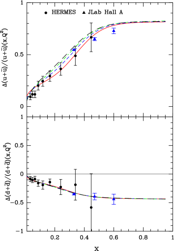
Another important earlier prediction concerns the Deep Inelastic Scattering (DIS) asymmetries, more precisely $(\Delta u(x,Q^{2})+\Delta\bar{u}(x,Q^{2}))/(u(x,Q^{2}+\bar{u}(x,Q^{2}))$ and $(\Delta d(x,Q^{2})+\Delta\bar{d}(x,Q^{2}))/(d(x,Q^{2})+\bar{d}(x,Q^{2}))$, shown in Fig. 1. Note that the data from HERMES hermes1 -hermes3 and Jlab JLab1 -JLab2 , so far, are in agreement with these predictions at low $x<0.6$. In the high $x$ region our prediction differs from those which impose, for both quantities, the value one for $x=1$. This is another challenge, since only up to $x=0.6$, they have been measured at JLab JLab1 -JLab2 ..

Figure 1: BS15 Bourrely:2015kla predicted ratios $(\Delta u(x,Q^{2})+\Delta\bar{u}(x,Q^{2}))/(u(x,Q^{2}+\bar{u}(x,Q^{2}))$ and $(\Delta d(x,Q^{2})+\Delta\bar{d}(x,Q^{2}))/(d(x,Q^{2}+\bar{d}(x,Q^{2}))$, versus $x$, at $Q^{2}(\mbox{GeV}^{2})=$ 1 solid , 10 dashed , 100 dashed-dotted, 1000 long-dashed. Experiments: HERMES hermes1 -hermes3 , Jlab JLab1 -JLab2 .

There are two more important consequences which relate unpolarized and helicity distributions, namely for quarks

$$xu(x,Q^{2})-xd(x,Q^{2})=x\Delta u(x,Q^{2})-x\Delta d(x,Q^{2})>0,$$ (15)

and similarly for antiquarks

$$x\bar{d}(x,Q^{2})-x\bar{u}(x,Q^{2})=x\Delta\bar{u}(x,Q^{2})-x\Delta\bar{d}(x,Q^{2})>0.$$ (16)

This means that the flavor asymmetry of the light antiquark distributions is the same for the corresponding helicity distributions, as noticed long time ago bbs-rev (see also ref. sala17 ).
Now let us come back to all these components $xu_{+}(x,Q^{2}),...x\bar{u}_{-}(x,Q^{2})$ and more precisely to their $x$-behavior. It is clear that $xu_{+}(x,Q^{2})$ is the largest one and they are all monotonic decreasing functions of $x$ at least for $x>0.2$, outside the region dominated by the diffractive contribution.
Similarly $x\bar{d}_{-}(x\,Q^{2})$ is the largest of the antiquark components.
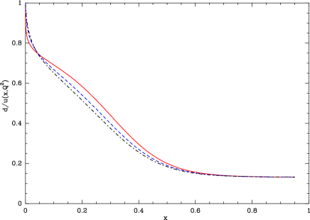
Therefore if one considers the ratio $d(x,Q^{2})/u(x,Q^{2})$, its value is one at $x=0$, because the diffractive contribution dominates and, due to the monotonic decreasing property, it decreases for an increasing $x$.
This falling $x$-behavior has been verified experimentaly from the ratio of the DIS structure functions $F_{2}^{d}/F_{2}^{p}$ and the charge asymmetry of the $W^{\pm}$ production in $\bar{p}p$ collisions Kuhlmann:1999sf .
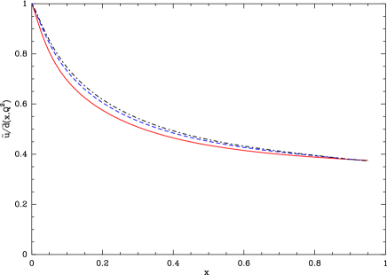
Similarly if one considers the ratio $\bar{u}(x,Q^{2})/\bar{d}(x,Q^{2})$, its value is one at $x=0$, because the diffractive contribution dominates and, due to the monotonic decreasing property, it also decreases for an increasing $x$.
By looking at the curves of Figure 2, one sees similar behaviors. In both cases in the vicinity of $x=0$ one has a sharp behavior due to the fact that the diffractive contribution dominates and in the high $x$ region there is a flattening out above $x\simeq 0.6$. It is remarkable to observe that these ratios have almost no $Q^{2}$ dependence.

Figure 2: The ratios $d(x,Q^{2})/u(x,Q^{2})$ (${\it left}$) and $\bar{u}(x,Q^{2})/\bar{d}(x,Q^{2})$ (${\it right}$) versus $x$ for $Q^{2}\mbox{GeV}^{2}=$ 1 solid , 10 dashed , 100 dashed-dotted, from BS15 Bourrely:2015kla .

To conclude one predicts a monotonic increase of the ratio $\bar{d}(x,Q^{2})/\bar{u}(x,Q^{2})$. This was first observed in the low $x$ region by the E866/NuSea collaboration E866a -E866b and very recently there is a serious indication from the preliminary results of the SeaQuest collaboration, that this trend persists beyond $x=0.2$ reimer .

V A toy model for gluon distributions

In the BS15 version of the model Bourrely:2015kla , the unpolarized gluon is parametrized as a Bose-Einstein function with a zero potential value and no diffractive part is included:

$$xG(x,Q^{2}_{0})=\frac{A_{G}x^{b_{G}}}{\exp(x/\bar{x})-1}~{},$$ (17)

where $A_{G}=36.778$ is determined by the momentum sum rule. The polarized gluon distribution involves also a Bose-Einstein function but requires an extra factorized function whose origin is discussed in Refs. bourr16 ; bs2015 , so its expression is given by:

$$x\Delta G(x,Q^{2}_{0})=\frac{\tilde{A}_{G}x^{\tilde{b}_{G}}}{(1+c_{G}x^{d_{G}})}\!\cdot\!\frac{1}{\exp(x/\bar{x})-1}\,,$$ (18)

where $\tilde{A}_{G}=26.887$. Contrary to the quarks situation these expressions are not directly related and so have to be determined independently from specific experimental data. Coming back to the model structure this is not exactely true because their determination is influenced by unpolarized and polarized quarks which are related, nevertheless, a more direct relation will reinforce the model structure.

Inside a proton at high energy beside the presence of 2 u + d quarks there exists a collection of $q-\bar{q}$ pairs and gluons. It is also know that a quark-antiquark pair can annihilate into 2 gluons. It seems natural to suppose that a $q-\bar{q}$ pair should behave like a composite boson and so could have a relation with the gluon field. In this case one should find that in a QCD process involving gluons, for instance in structure functions, one can replace the gluon by a $q-\bar{q}$ pair, leading to a new test for the antiquarks since the quarks are well established.
For this purpose two new formulas are defined for the unpolarized and polarized gluon which play the role of a toy model at the input scale. In these formulas $q$ and $\bar{q}$ contain only the non diffractive part of Eqs. (1, 2) and to comply with the previous definitions (17, 18), their expressions are now given by:

$$xG(x,Q^{2}_{0}) = A_{q\bar{q}}(xux\cdot x\bar{u}+xd\cdot x\bar{d}+xs\cdot x\bar{s})[x,Q^{2}_{0}]\,,$$ (19)

$$x\Delta G(x,Q^{2}_{0}) = A_{\delta q\bar{q}}(x\Delta u\cdot x\Delta\bar{u}+x\Delta d\cdot x\Delta\bar{d}+x\Delta s\cdot x\Delta\bar{s})[x,Q^{2}_{0}]\,.$$ (20)

Let us remark that the two formulas (19,20) although they contain the product of 2 Fermi functions both are evolved as a boson, so the result is not the evolution of the product of two Fermi distributions.
Also, in the expressions (17, 18) $G$ and $\Delta G$ are defined independently and are not related, while in the expressions (19,20) indeed they are because for a given flavour $q,\bar{q},\Delta q,\Delta\bar{q}$ are not independent. It has the consequence that the parton structure can be described with a very few number of basic constituents.

A fit at NLO of unpolarized and polarized DIS experimental data gives

in the case of BS15 parametrization Bourrely:2015kla

$$\chi^{2}=2860\quad\quad 2140pts\quad\quad 1.34\chi^{2}/pt$$ (21)

now with Eqs. (19,20) of the toy model a fit of the same set of data gives:

$$\chi^{2}=3013\quad\quad 2140pts\quad\quad 1.4\chi^{2}/pt\,,$$ (22)

the difference in $\chi^{2}$ is 5%. Restricted to the polarized structure functions $g_{1}^{p},g_{1}^{d},g_{1}^{n}$ with 271pts, BS15 gives a $\chi^{2}=323$, the toy model a $\chi^{2}=301$. Notice that in the original version the expression of $\Delta G$ requires 4 parameters, in this version only one normalization constant $A_{\delta q\bar{q}}$ is necessary, since $A_{G},~{}A_{q\bar{q}}$ are determined by the momentum sum rule, this difference confirms the interest for the gluons given by Eqs. (19,20)

In this new fit the potentials read

$$X_{u}^{+}=0.4616,\quad X_{u}^{-}=0.3166,$$

$$X_{d}^{+}=0.2530,\quad X_{d}^{-}=0.3062,$$

$$X_{s}^{+}=0.007896,\quad X_{s}^{-}=00982,$$

$$b_{q}=0.491,\quad\bar{b}_{q}=1.123,$$

$$b_{s}=0.0044,\quad\bar{b}_{s}=0.08,$$

$$\bar{x}=0.0944\,.$$ (23)

The new result for the potential values are close to the previous ones (7) and still satisfy the previous hierarchy (10).

$$X_{u}^{+}>X_{d}^{-}\sim X_{u}^{-}>X_{d}^{+}\,,$$ (24)

so the properties discussed in sec. IV remain valid.

For the normalization constants one obtains $A_{q\bar{q}}=23.882$, $A_{\delta q\bar{q}}=18.99$.

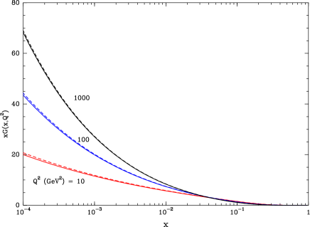
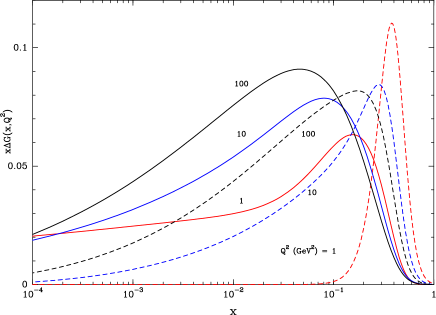
In Figure 3 a plot is given for some results associated with the unpolarized and polarized gluon in the case of BS15 parametrization (17, 18) (dashed curves) and the toy model (19, 20) (solid curves). The distributions behavior is very similar, the polarized case which is more sensitive to the gluon structure looks slightly different but when combined with the polarized quarks give an excellent description of the polarized structure functions (see the $\chi^{2}$ discussed above). To conclude this part devoted to the statistical model, the present formulas used as a toy parametrization of unpolarized and polarized gluons give an equivalent description of the original model, and they represent also a new test for the antiquarks PDFs since the quarks PDFs are well established. In QCD calculations Mellin transforms are sometime involved, the Mellin transform of a Fermi function for fermions and bosons are mathematically related srivast11 , which is an encouraging sign for our new definition of gluons.

Figure 3: Comparison of $xG(x,Q^{2})$ computed from BS15 Bourrely:2015kla (dashed) and the toy model (solid) (${\it left}$). Same comparison for $x\Delta G(x,Q^{2})$ (${\it right}$) versus $x$ for $Q^{2}=1,10,100\mbox{GeV}^{2}$.

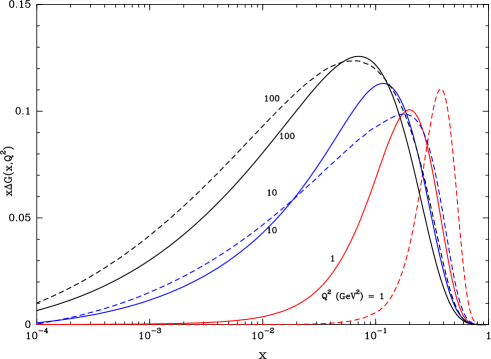
One can ask the question if the previous formulation can be applied to another model. In the domain of polarized PDFs the DSSV model dssv1 is a reference, so it becomes of interest to test this polarized version inside the toy model taking DSSV as input in Eq. (20). There is a difference between the statistical model and DSSV model due to the fact that in the statistical model unpolarized and polarized PDFs are related which is not the case with DSSV. Polarized quarks, antiquarks and gluon of flavor $i$ are defined in DSSV at the input scale $\mu_{0}$ by the expressions Eq. (28) of Ref. dssv1 namely

$$x\Delta f_{i}(x,\mu^{2}_{0})=N_{i}x^{\alpha_{i}}(1-x)^{\beta_{i}}(1+\gamma_{i}\sqrt{x}+\eta_{i}x)\,.$$ (25)

More serious constraint on the polarized gluon can be obtained from the double-spin asymmetry in jet production $A_{LL}^{jet}$ with the modified expression for the polarized DSSV gluon dssv2

$$x\Delta g(x,Q_{0}^{2})=N_{g}x^{\alpha_{g}}(1-x)^{\beta_{g}}\left(1+\eta_{g}x^{\kappa_{g}}\right)\,.$$ (26)

In order to test the toy model with the polarized gluon (20) one adopts the strategy to fit the same polarized data previously used taking Eqs. (25) for the quarks and Eq. (20) for the polarized gluon. For simplicity the quarks the number of free parameter is restricted to $N_{i},\eta_{i}$, while $\alpha_{i},\beta_{i},\gamma_{i},$ are held fixed to their original values (see Table II of Ref. dssv1 ).

flavor $i$	$N_{i}$	$\alpha_{i}$	$\beta_{i}$	$\gamma_{i}$	$\eta_{i}$
$u+\bar{u}$	0.403	0.692	3.34	-2.18	21.38
$d+\bar{d}$	-0.023	0.164	3.89	22.40	83.80
$\bar{u}$	4.83	0.692	10.0	0	24.97
$\bar{d}$	-0.147	0.164	10.0	0	98.94
$s=\bar{s}$	-0.019	0.164	10.0	0	-23.03

Table 1: Parameters describing NLO ($\overline{\mathrm{MS}}$) $x\Delta f_{i}$ in Eq. (25) at the input scale $\mu_{0}=1\,\mathrm{GeV}$, using the toy model

For the polarized gluon one obtains a normalization coefficient $A_{\delta q\bar{q}}=-0.078$. With a $\chi^{2}=235$ for 271pts the quality of the polarized fit is similar to the previous statistical model. Here again the five parameters introduced in Eq. (26) are reduced to one. A plot of the polarized gluon for three $Q^{2}$ values is shown in Fig. 4 for the original DSSV model (dashed curve) and the toy model (solid curve).

Figure 4: Comparison of $x\Delta G(x,Q^{2})$ versus $x$ for $Q^{2}=1,10,100\mbox{GeV}^{2}$ calculated with the toy DSSV (solid) and the orignal one (dashed).

Now our purpose is to show that the polarized gluon discussed above offers a good exploratory domain for the parton structure. Beginning with the statistical model, it was natural to associate to the gluon a Bose-Einstein expression such that

$$x\Delta G(x,Q^{2}_{0})=\tilde{A}_{G}x^{\tilde{b}_{G}}\!\cdot\!\frac{1}{\exp(x/\bar{x})-1}\,,$$ (27)

this original expression was unable to describe the double-spin asymmetry of the one-jet inclusive production $A_{LL}^{jet}$ in the near forward rapidity region as a function of $p_{T}$ within the domain 5 $\leq p_{T}\leq$ 30GeV measured by the STAR Collaboration at BNL-RHIC abelev06 . To obtain a good description the polarized gluon was modified according to Eq. (18).
It turns out that the extra multiplicative function $\frac{1}{(1+c_{G}x^{d_{G}})}$ has the behavior of a logistic function or activation function used in neural network bourr16

$$S(x)=\frac{1}{1+e^{-e_{G}x+h_{G}}}\,,$$ (28)

so one can write the polarized gluon as:

$$x\Delta G(x,Q^{2}_{0})=S(x)\frac{\tilde{A^{\prime}}_{G}x^{b_{G}}}{\exp(x/\bar{x})-1}\,.$$ (29)

The physical interpretation of this new formula means that the incoming momentum is collected now by means of a Bose-Einstein distribution and then filtered by an activation function to produce the gluon probability distribution.
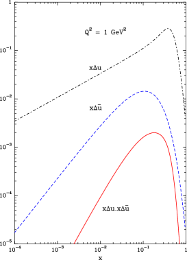
The toy model defined above proceeds along the same line, a polarized gluon is built in terms of a composite made of known physical functions namely the PDFs associated with their probability. In Fig. 5 the example of $u$, $\bar{u}$ quarks where their probabilities product generates a component of the gluon polarized PDF. The resulting effect of the toy model is perfectly compatible with experimental data for both the statistical and DSSV models.

Figure 5: Quark $u$ contribution to the polarized $\Delta G$ following the toy expression (20).

To summarize the discussion on the different expressions so far defined in (20),(27)-(29) our objective was to replace an arbitrary function by a physical quantity perfectly justified in the context of the model.
One knows that $\Delta G$ gives an important contribution to the proton spin sum rule. A study of this effect is presented in Fig. 3 of Ref. bs2015 using the gluon defined by Eq. (18). One sees that just above $Q^{2}=100\mbox{GeV}^{2}$ the value of the spin sum rule 1/2 is saturated, the same calculation performed with the toy gluon Eq. (20) gives a saturation for $Q^{2}$ around 1000GeV², which corresponds to a significant improvement.

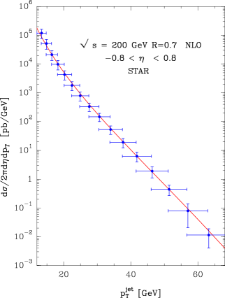
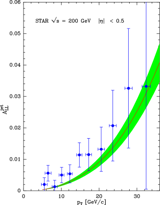
Finally, one would like to present a new test of the toy gluon distribution in a pure hadronic reaction and compute the double-helicity asymmetry $A^{jet}_{LL}$ discussed above. It is important to remark that the asymmetry calculation requires both the knowledge of the unpolarized and polarized gluon distributions (19)-(20). In Fig. 6 our prediction is compared with these high-statistics data points and the agreement is very reasonable.

Figure 6: [left] Inclusive differential cross section for $p+p\rightarrow jet+X$ at $\sqrt{s}$ = 200 GeV versus jet $p_{T}$ calculated with the unpolarized toy gluon Eq. (19). [right] The longitudinal double-spin asymmetry $A_{LL}$ in $\overrightarrow{p}+\overrightarrow{p}\rightarrow jet+X$ at $\sqrt{s}$ = 200 GeV versus jet $p_{T}$ calculated with the polarized toy gluon Eq. (20). Data STAR experiment Adamczyk:2014xyw .

VI Conclusion

Our purpose was to show that a statistical model offers a unique framework to build quarks structure whose properties are clearly defined by parameters related to physical quantities in the PDFs expressions. The thermodynamical potential which are the master parameters generate definite properties of the quarks PDFs confirmed by experimental structure functions.

This prediction results from the following characteristic features of the statistical approach:
- the PDF helicity components defined by Fermi-Dirac expressions are the building blocks of the unpolarized and polarized PDFs.
- the thermodynamical potentials satisfy a hierarchy relation given by Eq. (10) which imposes specific properties on the distribution functions.
- the expressions between quark and antiquarks obtained allow to relate the behavior of the ratios $xd(x,Q^{2})/xu(x,Q^{2})$ and $x\bar{u}(x,Q^{2})/x\bar{d}(x,Q^{2})$.
- a toy model has been defined for the gluon in terms of unpolarized and polarized quarks distributions which produces equivalent results to the original gluon parametrizations but with only one free normalization parameter. In addition this toy model gives for the gluon made with basic fermion helicity components a relation between unpolarized and polarized gluons distributions which was not the case in the original version of the model.

It is clear that our model is able to explain a large set of unpolarized and polarized experimental Deep Inelastic Scattering data. Of course the predictions which can be made in view of future experiments depend on the present values of the parameters so it is a challenge for the model to be confimed by new experiments.

To conclude our statistcal approach not only provides numerical PDFs values compatible with experimental data but also gives a coherent model of the quarks structure at the fundamental level of helicity distributions.

References

- (1) S. Dulat et al., Phys. Rev. D 93, 033006 (2016).
- (2) L.A. Harland-Lang, A.D. Martin, P. Motylinski and R.S. Thorne, Eur. Phys. J. C 75, 204 (2015).
- (3) C. Bourrely, F. Buccella and J. Soffer, Eur. Phys. J. C 23, 487 (2002).
- (4) G.P. Salam and J. Rojo, Comput. Phys. Commun, 180, 120 (2009), (arXiv:0804.3755 [hep-ph])
- (5) C. Bourrely, J. Soffer, Nucl. Phys. A 941, 307 (2015).
- (6) L. Adamczyk, et al., STAR Collaboration, Phys. Rev. Lett. 113, 072301 (2014).
- (7) HERMES Collaboration, K. Ackerstaff et al., Phys. Lett.B 404, 383 (1997).
- (8) HERMES Collaboration, K. Ackerstaff et al., Phys. Lett. B 464, 123 (1999).
- (9) HERMES Collaboration A. Airapetian et al., Phys. Lett. B 442, 484 (1998).
- (10) X, Zheng et al., Phys. Rev. C 70, ) 065207 (2004).
- (11) X, Zheng et al., Phys. Rev. Lett. 92, 012004 (2004).
- (12) C. Bourrely, J. Soffer and F. Buccella, Eur. Phys. J. C 41, 327 (2005) 327.
- (13) M. Salajegheh et al., Phys. Rev. C 96, 065205 (2017).
- (14) S. Kuhlmann, et al., Phys. Lett. B 476, 291 (2000).
- (15) FNAL Nusea Collaboration, E. A. Hawker et al., Phys. Rev. Lett. 80, 3715 (1998).
- (16) J. C. Peng et al., Phys. Rev. D 58, 092004 (1998).
- (17) P. Reimer, The Quest for the Origin of the Proton’s Sea Invited talk at ”DIFFRACTION 2016”, Sept. 02 - 08, 2016, Acireale, Sicily (Italy), AIP Conference Proceedings (2017).
- (18) C. Bourrely, Scholar’s Press, Verlag Publisher, 2016; see also [arXiv:1507.03752].
- (19) H.M. Srivastava, et al., Russ. J. Math. Phys. 11, 107 (2011).
- (20) D. de Florian, R. Sassot, M. Stratmann and W. Vogelsang, Phys. Rev. D 80, ) 034030 (2009.
- (21) D. de Florian, R. Sassot, M. Stratmann and W. Vogelsang, Phys. Rev. Lett. 113, 012001 (2014).
- (22) B.I. Abelev, et al., Phys. Rev. Lett. 97, 252001 (2006).
- (23) C. Bourrely and J. Soffer, Phys. Lett. B 740, 168 (2015).