GCA-$\mathcal{H}^{2}$ matrix compression for electrostatic simulations

Abstract

We consider a compression method for boundary element matrices arising in the context of the computation of electrostatic fields. Green cross approximation combines an analytic approximation of the kernel function based on Green’s representation formula and quadrature with an algebraic cross approximation scheme in order to obtain both the robustness of analytic methods and the efficiency of algebraic ones. One particularly attractive property of the new method is that it is well-suited for acceleration via general-purpose graphics processors (GPUs).

1 Introduction

Boundary integral formulations are particularly useful when dealing with electrostatic exterior domain problems: we only have to construct a mesh for the boundary of the domain, and once an integral equation on this boundary has been solved, we can directly evaluate the electrostatic field in all points of the infinite domain by computing a surface integral.

Standard formulations typically lead to equations of the form

$$\int_{\partial\Omega}g(x,y)u(y)\,dy=\lambda u(x)+\int_{\partial\Omega}\frac{\partial g}{\partial n_{y}}(x,y)v(y)\,dy$$

for all $x\in\partial\Omega$, where $\Omega\subseteq\mathbb{R}^{3}$ is a domain, $\lambda\in\mathbb{R}$, $u$ and $v$ are scalar functions on the boundary $\partial\Omega$, and

$$g(x,y)=\frac{1}{4\pi\|x-y\|}$$

is the fundamental solution of Laplace’s equation.

Discretization by Galerkin’s method with basis functions $(\varphi_{i})_{i\in\mathcal{I}}$ leads to a matrix $G\in\mathbb{R}^{\mathcal{I}\times\mathcal{I}}$ given by

$$g_{ij}=\int_{\partial\Omega}\varphi_{i}(x)\int_{\partial\Omega}g(x,y)\varphi_{j}(y)\,dy\,dx$$ (1)

for all $i,j\in\mathcal{I}$, and all of these coefficients are typically non-zero.

Working directly with the matrix $G$ is unattractive, since for $n:=\#\mathcal{I}$ basis functions, we would have to store $n^{2}$ coefficients and quickly run out of memory.

This problem can be fixed by taking advantage of the properties of the kernel function $g$: analytic approximation schemes like the fast multipole method [14, 11], Taylor expansion [13], or interpolation [5, 8] replace $g$ in suitable subdomains of the boundary $\partial\Omega$ by a short sum

$$g(x,y)\approx\sum_{\nu=1}^{k}a_{\nu}(x)b_{\nu}(y)$$

that leads to a low-rank approximation of corresponding submatrices of $G$, while algebraic schemes like the adaptive cross approximation (ACA) [17, 1, 2] or rank-revealing factorizations [9] directly construct low-rank approximations based on the matrix entries.

Hybrid approximation schemes like generalized fast multipole methods [10, 18] or hybrid cross approximation (HCA) [6] combine the concepts of analytic and algebraic approximation in order to obtain the near-optimal compression rates of algebraic methods while preserving the stability and robustness of analytic techniques.

Our algorithm falls into the third category: Green cross approximation (GCA) combines an analytic approximation based on Green’s representation formula with adaptive cross approximation (ACA) to obtain low-rank approximations of submatrices. In order to improve the efficiency, we employ GCA in a recursive fashion that allows us to significantly reduce the storage requirements without losing the method’s fast convergence.

While all of these technique allow us to handle the boundary integral equation more or less efficiently, analytic methods and some of the hybrid methods can also be used to speed up the subsequent evaluation of the electrostatic field in arbitrary points of $\Omega$.

2 Green quadrature

In order to find a data-sparse approximation of $G$, we consider a domain $\tau\subseteq\mathbb{R}^{3}$ and a superset $\omega\subseteq\mathbb{R}^{3}$ such that the distance from $\tau$ to the boundary $\partial\omega$ of $\omega$ is non-zero. For any $y\in\mathbb{R}^{3}\setminus\overline{\omega}$, the function $x\mapsto g(\cdot,y)$ is harmonic in $\omega$, so we can apply Green’s representation formula (also known as Green’s third identity) to obtain

$$g(x,y)=\int_{\partial\omega}g(x,z)\frac{\partial g}{\partial n_{z}}(z,y)-\frac{\partial g}{\partial n_{z}}(x,z)g(z,y)\,dz$$

for all $x\in\tau$ and $y\in\mathbb{R}^{3}\setminus\overline{\omega}$. If the distances between $\partial\omega$ and $\tau$ and between $\partial\omega$ and $y$ are sufficiently large, the integrand is smooth, and we can approximate the integral by a quadrature rule to find

$$g(x,y)\approx\sum_{\nu=1}^{k} w_{\nu}g(x,z_{\nu})\frac{\partial g}{\partial n_{z}}(z_{\nu},y)$$

$$- w_{\nu}\frac{\partial g}{\partial n_{z}}(x,z_{\nu})g(z_{\nu},y)$$ (2)

with weights $w_{\nu}$ and quadrature points $z_{\nu}$, and in this approximation the variables $x$ and $y$ are separated.

This gives rise to a first low-rank approximation of $G$: given subsets $\widehat{\tau},\widehat{\sigma}\subseteq\mathcal{I}$ of the index set, we can introduce axis-parallel boxes

$$\tau \supseteq\bigcup_{i\in\widehat{\tau}}\mathop{\operatorname{supp}}\nolimits\varphi_{i}, \sigma \supseteq\bigcup_{j\in\widehat{\sigma}}\mathop{\operatorname{supp}}\nolimits\varphi_{j}$$

containing the supports of the corresponding basis functions, and if these boxes are well-separated, we can find a superset $\omega$ of $\tau$ such that its boundary $\partial\omega$ is sufficiently far from both $\tau$ and $\sigma$. Replacing $g$ in the definition (1) of the Galerkin matrix by the quadrature-based approximation leads to a factorized approximation

$$G|_{\widehat{\tau}\times\widehat{\sigma}}\approx A_{\tau\sigma}B_{\tau\sigma}^{*},$$

with $A_{\tau\sigma}\in\mathbb{R}^{\widehat{\tau}\times 2k}$ and $B_{\tau\sigma}\in\mathbb{R}^{\widehat{\sigma}\times 2k}$, so the rank of the approximation is bounded by $2k$.

The matrix coefficients are given by

$$a_{\tau\sigma,i\nu} =\sqrt{w_{\nu}}\int_{\partial\Omega}g(x,z_{\nu})\varphi_{i}(x)\,dx,$$

$$a_{\tau\sigma,i(\nu+k)} =-d_{\tau}\sqrt{w_{\nu}}\int_{\partial\Omega}\frac{\partial g}{\partial n_{z}}(x,z_{\nu})\varphi_{i}(x)\,dx,$$

$$b_{\tau\sigma,j\nu} =\sqrt{w_{\nu}}\int_{\partial\Omega}\frac{\partial g}{\partial n_{z}}(z_{\nu},y)\varphi_{j}(y)\,dy,$$

$$b_{\tau\sigma,j(\nu+k)} =\frac{\sqrt{w_{\nu}}}{d_{\tau}}\int_{\partial\Omega}g(z_{\nu},y)\varphi_{j}(y)\,dy,$$

where the scaling parameter $d_{\tau}=\mathop{\operatorname{diam}}\nolimits(\tau)$ serves to balance the different scaling behaviour of the kernel function and its normal derivative.

Figure 1: Relative error of the Green quadrature approximation compared to the storage requirements

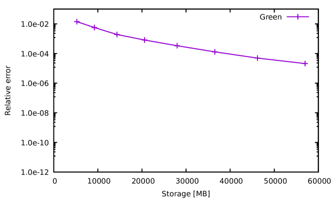
We apply the approximation scheme to a polygonal approximation of the unit sphere by $n=32\,768$ triangles, choosing piecewise constant basis functions and the admissibility condition

$$\max\{\mathop{\operatorname{diam}}\nolimits(\tau),\mathop{\operatorname{diam}}\nolimits(\sigma)\}\leq 2\eta\mathop{\operatorname{dist}}\nolimits(\tau,\sigma)$$

with a parameter $\eta\in\mathbb{R}_{>0}$ to determine whether a submatrix $G|_{\widehat{\tau}\times\widehat{\sigma}}$ can be approximated.

Figure 1 shows the relative spectral error, estimated via the power iteration, as a function of the storage requirements. We can see that the convergence is quite disappointing, particularly since storing the entire matrix as a simple two-dimensional array requires only $8\,192$ MB of storage.

3 Green cross approximation

In order to make the approximation more efficient, we can apply adaptive cross approximation [1] to derive the algebraic counterpart of interpolation: this technique provides us with a small subset $\tilde{\tau}\subseteq\widehat{\tau}$ and a matrix $V_{\tau}\in\mathbb{R}^{\widehat{\tau}\times\tilde{\tau}}$ such that

$$V_{\tau}A_{\tau\sigma}|_{\tilde{\tau}\times 2k}\approx A_{\tau\sigma},$$

i.e., we can reconstruct $A_{\tau\sigma}$ using only a few of its rows. Since $A_{\tau\sigma}$ is a thin matrix, we can afford to use reliable pivoting strategies and do not have to rely on heuristics. We conclude

$$V_{\tau}G|_{\tilde{\tau}\times\widehat{\sigma}}\approx V_{\tau}A_{\tau\sigma}|_{\tilde{\tau}\times 2k}B_{\tau\sigma}^{*}\approx A_{\tau\sigma}B_{\tau\sigma}^{*}\approx G|_{\widehat{\tau}\times\widehat{\sigma}},$$

i.e., the algebraic interpolation can also be applied directly to the original matrix $G$ instead of the low-rank approximation. This is called a Green cross approximation (GCA).

It is important to keep in mind that the matrices $A_{\tau\sigma}$ only depend on $\tau$, but not on $\sigma$, so the cross approximation algorithm has to be performed only once for each $\tau$ and both the set $\tilde{\tau}$ and the matrix $V_{\tau}$ do not depend on $\sigma$.

Our modification has two major advantages: on one hand, the ranks are bounded by both the cardinality of $\widehat{\tau}$ and the number of quadrature points, so that the approximation can be far more efficient for small clusters. On the other hand, we can reach significantly higher accuracies, since the Green quadrature is only used to choose good “interpolation points” $\tilde{\tau}$, while the final approximation relies on the entries of the original matrix $G$.

Figure 2: Relative error of the Green quadrature approximation and the Green cross approximation (GCA) compared to the storage requirements

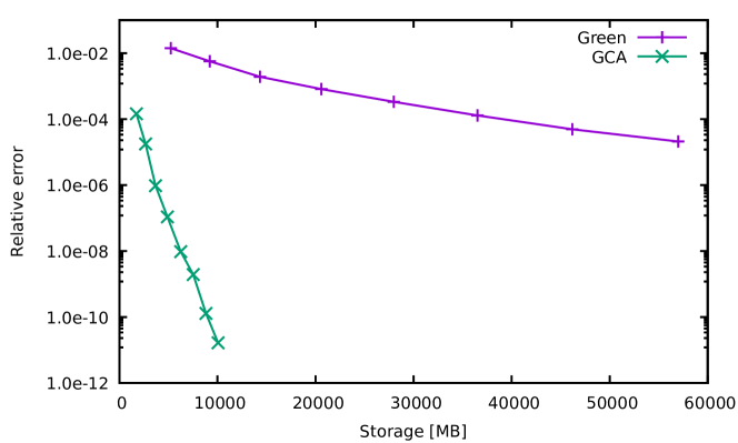
Figure 2 illustrates that combining cross approximation with Green quadrature significantly improves the performance: we can reach fairly high accuracies with moderate storage requirements.

4 $\mathcal{H}^{2}$-matrices

Since Green’s formula is symmetric with respect to $\tau$ and $\sigma$, we can also apply the representation formula to a superset of $\sigma$ and combine the formular with quadrature and cross approximation to obtain a subset $\tilde{\sigma}\subseteq\widehat{\sigma}$ and $V_{\sigma}\in\mathbb{R}^{\widehat{\sigma}\times\tilde{\sigma}}$ with

$$G|_{\widehat{\tau}\times\widehat{\sigma}}\approx G|_{\widehat{\tau}\times\tilde{\sigma}}V_{\sigma}^{*}.$$

Together with the approximation for $\tau$ introduced before, we obtain the symmetric factorization

$$G|_{\widehat{\tau}\times\widehat{\sigma}}\approx V_{\tau}G|_{\tilde{\tau}\times\tilde{\sigma}}V_{\sigma}^{*},$$

and this turns out to be very efficient, since $G|_{\tilde{\tau}\times\tilde{\sigma}}$ is usually significantly smaller than $G|_{\widehat{\tau}\times\widehat{\sigma}}$.

We can improve the construction further by representing the basis matrices $V_{\tau}$ and $V_{\sigma}$ in a hierarchy: assume that $\widehat{\tau}$ is subdivided into disjoint subsets $\widehat{\tau}_{1}$ and $\widehat{\tau}_{2}$ and that matrices $V_{\tau_{1}},V_{\tau_{2}}$ and subsets $\tilde{\tau}_{1}\subseteq\widehat{\tau}_{1},\tilde{\tau}_{2}\subseteq\widehat{\tau}_{2}$ have already been constructed. We let $\tilde{\tau}_{1,2}:=\tilde{\tau}_{1}\cup\tilde{\tau}_{2}$ and observe

$$A_{\tau\sigma} =\begin{pmatrix}A_{\tau\sigma}|_{\widehat{\tau}_{1}\times 2k}\\ A_{\tau\sigma}|_{\widehat{\tau}_{2}\times 2k}\end{pmatrix}\approx\begin{pmatrix}V_{\tau_{1}}A_{\tau\sigma}|_{\tilde{\tau}_{1}\times 2k}\\ V_{\tau_{2}}A_{\tau\sigma}|_{\tilde{\tau}_{2}\times 2k}\end{pmatrix}=\begin{pmatrix}V_{\tau_{1}}&\\ &V_{\tau_{2}}\end{pmatrix}A_{\tau\sigma}|_{\tilde{\tau}_{1,2}\times 2k}.$$

If we now apply cross approximation to the right factor $\widehat{A}_{\tau\sigma}:=A_{\tau\sigma}|_{\tilde{\tau}_{1,2}\times 2k}$, we obtain a subset $\tilde{\tau}\subseteq\tilde{\tau}_{1,2}$ and a matrix $\widehat{V}_{\tau}\in\mathbb{R}^{\tilde{\tau}_{1,2}\times\tilde{\tau}}$ with

$$\widehat{V}_{\tau}\widehat{A}_{\tau\sigma}|_{\tilde{\tau}\times 2k}\approx\widehat{A}_{\tau\sigma}$$

and therefore

$$A_{\tau\sigma} \approx\begin{pmatrix}V_{\tau_{1}}&\\ &V_{\tau_{2}}\end{pmatrix}\widehat{A}_{\tau\sigma}\approx\begin{pmatrix}V_{\tau_{1}}&\\ &V_{\tau_{2}}\end{pmatrix}\widehat{V}_{\tau}A_{\tau\sigma}|_{\tilde{\tau}\times 2k}=V_{\tau}A_{\tau\sigma}|_{\tilde{\tau}\times 2k},$$

where the basis matrix

$$V_{\tau}:=\begin{pmatrix}V_{\tau_{1}}&\\ &V_{\tau_{2}}\end{pmatrix}\widehat{V}_{\tau}$$

can be expressed in the form

$$V_{\tau} =\begin{pmatrix}V_{\tau_{1}}E_{\tau_{1}}\\ V_{\tau_{2}}E_{\tau_{2}}\end{pmatrix}, E_{\tau_{1}} :=\widehat{V}_{\tau}|_{\tilde{\tau}_{1}\times\tilde{\tau}}, E_{\tau_{2}} :=\widehat{V}_{\tau}|_{\tilde{\tau}_{2}\times\tilde{\tau}}.$$

If we use this factorized representation of the matrices $V_{\tau}$, we only have to store $V_{\tau}$ if $\widehat{\tau}$ has no subsets, while we use the substantially smaller transfer matrices $E_{\tau_{1}},E_{\tau_{2}}$ for all other index sets.

Since $\tilde{\tau}_{1,2}$ is usually significantly smaller than $\widehat{\tau}$, this construction is faster than the straightforward GCA approach, and the recursive use of transfer matrices reduces the storage requirements. The resulting approximation of $G$ is known as an $\mathcal{H}^{2}$-matrix [12, 7, 3], and it can be proven to have linear complexity with respect to the matrix dimension $n$.

Figure 3: Relative error of the Green quadrature approximation, GCA, and GCA-$\mathcal{H}^{2}$ compared to the storage requirements

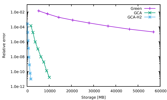
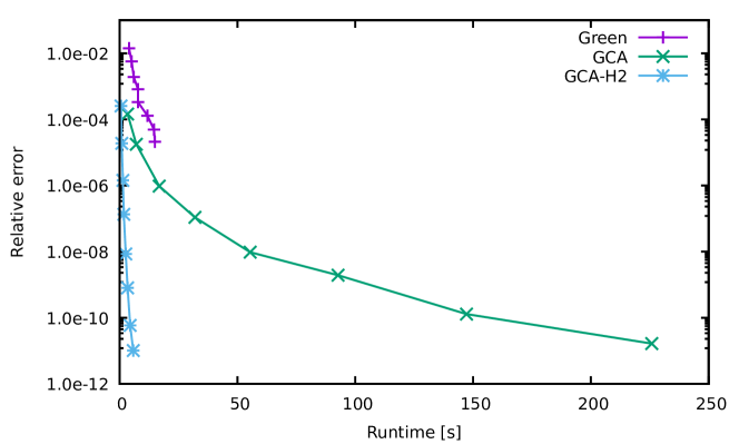
The resulting GCA-$\mathcal{H}^{2}$-matrix compression algorithm can be proven to converge exponentially and to have almost optimal complexity [4]. Indeed, Figure 4 illustrates that the new algorithm requires only a few seconds to compute a highly accurate approximation.

Figure 4: Relative error of the Green quadrature approximation, GCA, and GCA-$\mathcal{H}^{2}$ compared to the setup time

5 Linear basis functions

So far, we have only considered piecewise constant basis functions in our experiments, since they make it particularly simple to approximate the entries of the matrix $G$. If the solution of the integral equation is smooth, it is generally a good idea to employ basis functions of higher order to obtain faster convergence.

One step up from piecewise constant basis functions are piecewise linear functions, and we choose continuous piecewise linear functions, both in order to reduce the number of unknown variables and to be able to work with integral operators that require an $H^{1/2}$-conforming trial space. The trial space is spanned by nodal basis functions $\varphi_{i}$: $\varphi_{i}$ is continuous, piecewise linear on each triangle, equal to one in the $i$-th vertex, and equal to zero in all other vertices.

The support of $\varphi_{i}$ consists of all triangles that contain the $i$-th vertex, therefore computing the entry $g_{ij}$ of the matrix requires us to compute integrals on all pairs of triangles $t\times s$ where $t$ belongs to the support of $\varphi_{i}$ and $s$ to the support of $\varphi_{j}$:

$$g_{ij}=\sum_{t\subseteq\mathop{\operatorname{supp}}\nolimits\varphi_{i}}\sum_{s\subseteq\mathop{\operatorname{supp}}\nolimits\varphi_{j}}\int_{t}\varphi_{i}(x)\int_{s}g(x,y)\varphi_{j}(y)\,dy\,dx.$$

Due to this property, the computation of one entry of the matrix with nodal basis functions can be significantly more computationally expensive than for a piecewise constant basis.

This problem can be somewhat mitigated by assembling the matrix triangle pair by triangle pair: we start with a zero matrix and loop over all pairs of triangles $t\times s$. For each pair, we evaluate the integrals for all of the triangles’ vertices and add the results to the appropriate matrix coefficients. Although the final result is the same, we consider each pair of triangles only once, and this allows us to re-use the values of the kernel function $g$ in the quadrature points for all combinations of basis functions. Since the evaluation of the transformed kernel function is the most computationally expensive part of the quadrature, this approach can make the entire construction far more efficient.

Unfortunately, our compression scheme does not need all of the matrix entries, only entries for subsets $\tilde{\tau}\times\tilde{\sigma}$ or $\hat{\tau}\times\hat{\sigma}$, so looping over all pairs of triangles would be a waste of time. Instead, we need an algorithm that determines only the required triangles and loops over them.

We typically store a matrix $G|_{\hat{\tau}\times\hat{\sigma}}$ by enumerating the row and column indices $\hat{\tau}=\{i_{1},\ldots,i_{n}\}$, $\hat{\sigma}=\{j_{1},\ldots,j_{m}\}$ with $n=\#\hat{\tau}$, $m=\#\hat{\sigma}$, and using a matrix in $\mathbb{R}^{n\times m}$. This means that it is not enough to find which triangles have to participate in our computation, we also have to determine which index numbers correspond to the triangles’ vertices.

Given a standard representation of the mesh, it is quite simple to determine for each index $i$ the set $T_{i}$ of triangles covering the support of the basis function $\varphi_{i}$. The challenge is to unify these sets for all basis functions corresponding to a subset $\hat{\tau}$ of indices. We use a variant of the well-known mergesort algorithm to handle this task: for example, assume that we have triangles

$$t_{1} =(1,2,3), t_{2} =(2,3,5), t_{3} =(4,1,3),$$

$$t_{4} =(6,5,2), t_{5} =(1,7,4), t_{6} =(7,6,1)$$

and are looking for the list of triangles for the vertex set $\hat{\tau}=\{1,6,4\}$. We have

$$T_{1} =\{t_{1},t_{3},t_{5},t_{6}\}, T_{6} =\{t_{4},t_{6}\}, T_{4} =\{t_{3},t_{5}\}.$$

We write the triangles for each vertex into rows of a matrix, where each row starts with the triangle, followed by three entries for its three vertices that are equal to the local index if this vertex is the current one or equal to the special symbol $\bot$ if it is not:

$$\begin{array}[]{r|rrr}t_{1}&1&\bot&\bot\\ t_{3}&\bot&1&\bot\\ t_{5}&1&\bot&\bot\\ t_{6}&\bot&\bot&1\\ \hline\cr t_{4}&2&\bot&\bot\\ t_{6}&\bot&2&\bot\\ \hline\cr t_{3}&3&\bot&\bot\\ t_{5}&\bot&\bot&3\end{array}$$

Now we apply the mergesort algorithm to sort the rows by the first column. If two rows have the same first column, i.e., if they correspond to the same triangle, the rows are combined: if a column has an index in one row and $\bot$ in the other, the combined row will have the index in this column. If the rows have $\bot$ in the same column, the combined row will, too. In our example, the result looks as follows:

$$\begin{array}[]{r|rrr}t_{1}&1&\bot&\bot\\ t_{3}&3&1&\bot\\ t_{4}&2&\bot&\bot\\ t_{5}&1&\bot&3\\ t_{6}&\bot&2&1\end{array}$$

Each triangle appears in exactly one row, and each row provides us with the local indices for all vertices of this triangle. The mergesort algorithm has a complexity of $\mathcal{O}(n\log n)$ if $n$ indices with $\mathcal{O}(1)$ triangles per index are used, therefore the overhead for finding the triangles and the local indices is low compared to the computational work for the quadrature itself.

6 Curved triangles

In our examples, linear basis function by themselves did reduce the storage requirements, but did not lead to faster convergence of the solution. Since the reason appears to be that the polygonal approximation of the smooth surface is insufficiently accurate, we consider replacing the piecewise linear parametrizations of the triangles by piecewise quadratic functions. This leads to curved triangles.

We implement these generalized triangles using the reference triangle $\hat{t}:=\{x\in\mathbb{R}^{2}\ :\ x_{1},x_{2}\geq 0,\ x_{1}+x_{2}\leq 1\}$ and quadratic parametrizations $\Phi_{t},\Phi_{s}:\hat{t}\to\mathbb{R}^{3}$ such that

$$\int_{t} \varphi_{i}(x)\int_{s}g(x,y)\varphi_{j}(y)\,dy\,dx$$

$$=\int_{\hat{t}}\gamma_{t}(\hat{x})\varphi_{i}(\Phi_{t}(\hat{x}))\int_{\hat{t}}g(\Phi_{t}(\hat{x}),\Phi_{s}(\hat{y}))\gamma_{s}(\hat{y})\varphi_{j}(\Phi_{s}(\hat{y}))\,d\hat{y}\,d\hat{x}$$

holds with the Gramians

$$\gamma_{t}(\hat{x}) =\left\|\frac{\partial\Phi_{t}}{\partial\hat{x}_{1}}(\hat{x})\times\frac{\partial\Phi_{t}}{\partial\hat{x}_{2}}(\hat{x})\right\|_{2}, \gamma_{s}(\hat{y}) =\left\|\frac{\partial\Phi_{s}}{\partial\hat{y}_{1}}(\hat{y})\times\frac{\partial\Phi_{s}}{\partial\hat{y}_{2}}(\hat{y})\right\|_{2}.$$

For the basis functions, we choose mapped nodal basis functions, i.e., $\varphi_{i}\circ\Phi_{t}$ and $\varphi_{j}\circ\Phi_{s}$ are nodal linear basis functions on the reference triangle $\hat{t}$, while $\varphi_{i}$ and $\varphi_{j}$ not necessarily linear themselves.

We can evaluate the double integral by using Sauter’s quadrature rule [15, 16], we only have to provide an efficient way of evaluating the parametrization and the Gramian in the quadrature points. For the parametrization, we simply use quadratic interpolation in the vertices and the midpoints of the edges. For the Gramian, we observe that the outer normal vector

$$n_{t}(\hat{x})=\frac{\partial\Phi_{t}}{\partial\hat{x}_{1}}(\hat{x})\times\frac{\partial\Phi_{t}}{\partial\hat{x}_{2}}(\hat{x})$$

is again a quadratic polynomial, so we can evaluate it also by interpolation once we have computed its values in the vertices and the midpoints. Once we have $n_{t}(\hat{x})$ at our disposal, computing $\gamma_{t}(\hat{x})=\|n_{t}(\hat{x})\|_{2}$ is straightforward. If we want to evaluate the double-layer potential operator and need the unit outer normal vector, we can obtain it by simply dividing $n_{t}(\hat{x})$ by $\gamma_{t}(\hat{x})$.

Figure 5: $L^{2}$ error compared to the storage requirements for constant and linear basis functions as well as plane and curved triangles

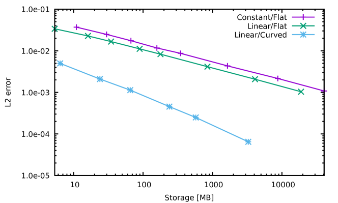
Figure 5 shows the $L^{2}$ error of the solution compared to the storage requirements for constant basis functions, linear basis functions on plane triangles, and linear basis functions on curved triangles. We can see that constant and linear basis functions on plane triangles converge at approximately the same rate, while curved triangles lead to a significantly improved rate of convergence and pronouncedly smaller errors for identical problem dimensions.

Figure 6: $L^{2}$ error compared to the setup time for constant and linear basis functions as well as plane and curved triangles

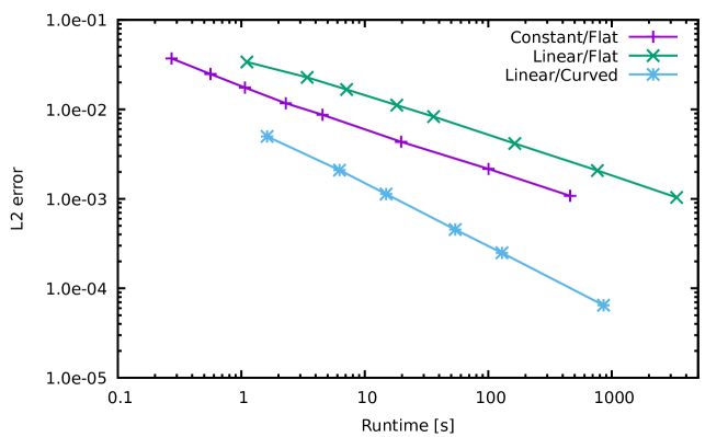
Figure 6 compares the $L^{2}$ error to the setup times for the three cases. As is to be expected, linear basis functions require far more time than constant basis functions, and curved triangles again take more time than plane ones. But we can also see that the combination of linear basis functions with curved triangles provides us with significantly lower $L^{2}$ errors, making the most sophisticated approach also the most efficient of the three.

If the surface and the solution are sufficiently smooth, we can choose collocation instead of Galerkin’s method for the discretization, i.e., define the matrix entries via

$$g_{ij}=\int_{\partial\Omega}g(x_{i},y)\varphi_{j}(y)\,dy,$$

where $x_{i}$ is a vertex of the mesh and $\varphi_{j}$ is a nodal basis function. Since collocation requires only a single instead of a double integral, the number of quadrature points is significantly smaller. Since the singularity is fixed at $y=x_{i}$, a simple Duffy transformation is sufficient to regularize the integral, and this makes the implementation quite straightforward.

Figure 7: $L^{2}$ error compared to the setup time for constant and linear basis functions as well as plane and curved triangles

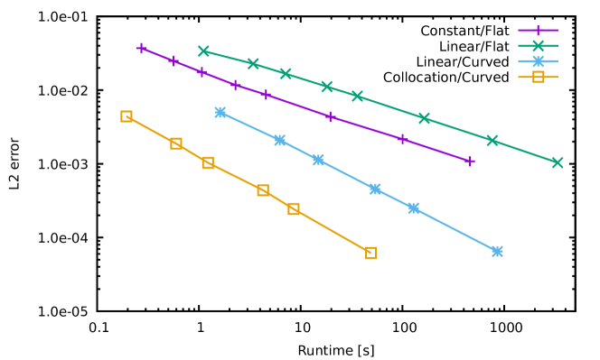
Figure 7 illustrates that collocation reduces the setup time by a factor of approximately ten compared to the Galerkin discretization without significantly changing the quality of the approximated solution.

7 GPU implementation

Modern computers are frequently equipped with powerful graphics processors that are (reasonably) programmable and can therefore help with certain computational tasks. These processors are frequently called general-purpose graphics processing units (GPGPUs or short GPUs) and differ substantially from standard processors (CPUs). In order to use GPUs to accelerate our algorithm, we have to take the architectural differences into account.

A first important difference is the way CPUs and GPUs handle data: high-end GPUs typically are connected to dedicated high-bandwidth memory. While a current CPU may reach a memory bandwidth of $60$ GBytes/s, modern GPUs provide up to $550$ GBytes/s. It has to be pointed out that the higher bandwidth comes at a price: while even desktop CPUs can access $64$ GBytes of RAM, with server CPUs accessing up to $1024$ GBytes, current GPUs are limited to $24$ GBytes of memory. In order to deal with large data sets, we have to move data between graphics memory and main memory, and these transfers are fairly slow.

The most important difference is the number of arithmetic units: while a 28-core CPU with 512-bit vector registers can perform $28\times 16=448$ double-precision floating-point operations per clock, high-end GPUS offer currently up to $4\,608$ arithmetic units that can work in parallel. Even taking differences in clock speeds into account, the theoretical computing power of GPUs is significantly larger than that of CPUs.

In order to control the large number of arithmetic units efficiently, GPUs restrict the ways these units can work. Current architectures follow what is known as the single instruction, multiple threads (SIMT) model: the computation is split into threads, frequently hundreds of thousands or millions, each with its own instruction pointer and local variables.

In order to keep the management of the threads simple, a fixed number of threads is bundled into a warp, e.g., $32$ or $64$ threads, depending on the architecture.

The GPU consists of multiple multiprocessors that can execute the instructions required by a warp. Each multiprocessor is assigned a certain number of warps. In each cycle, one of these warps and one of its instructions is chosen for execution. If the instruction pointer of a thread indicates the chosen instruction, it is executed, otherwise the thread remains idle during the current cycle.

This is a key difference between GPUs and CPUs: all threads running on a CPU are independent and can execute any instruction per cycle, while all threads in the same warp on a GPU have to execute the same instruction or do nothing.

If the control flow of the threads within one warp diverges, i.e., if all of the threads have to execute different instructions, only one of the instruction can be executed per cycle, allowing only one of the threads to advance. Obviously, having $63$ of $64$ arithmetic units idle for an extended period of time is not the best use of the available hardware.

8 GCA-$\mathcal{H}^{2}$ for GPUs

Let us now consider how to adapt our algorithm for execution on GPUs.

The computational work is dominated by three tasks:

• the construction of the leaf and transfer matrices $V_{\tau}$ and $E_{\tau}$ and the index sets $\tilde{\tau}$ by Green quadrature and cross approximation,

• the computation of the coupling matrices $G|_{\tilde{\tau}\times\tilde{\sigma}}$ for admissible blocks, and

• the computation of $G|_{\hat{\tau}\times\hat{\sigma}}$ for the remaining inadmissible blocks.

Although the entries of $A_{\tau\sigma}$ or $\widehat{A}_{\tau\sigma}$ involve no control-flow divergence and should therefore be well-suited for SIMT architectures, the highly adaptive nature of the cross approximation leads us to leave the first part of the algorithm to the CPU, where parallelization and vectorization can be employed to take full advantage of the available resources.

Once the sets $\tilde{\tau}$ and $\tilde{\sigma}$ are known, the computation of the entries of the matrices $G|_{\tilde{\tau}\times\tilde{\sigma}}$ and $G|_{\hat{\tau}\times\hat{\sigma}}$ requires no adaptivity whatsoever, so the second and third part of our algorithm can be expected to be ideally suited for GPUs.

Setting up the GPU to run a number of threads involves a certain amount of communication and management operations, therefore we should make sure that the number of threads is sufficiently high in order to minimize organizational overhead. Since our algorithm only works with small matrices that would not allow us to reach an adequate number of threads, we switch to an asynchronous execution model: instead of computing the entries of a matrix the moment it is encountered by our algorithm, the corresponding task is added to a list for later handling. Only once the list has grown enough to keep a sufficiently large number of threads busy, it is transferred to the GPU for execution.

This approach also allows us to handle different cases appearing in the numerical quadrature: we use Sauter’s quadrature rule [15, 16] to integrate the singular kernel function on pairs of triangles. Sauter’s algorithm requires different quadrature points (and even different numbers of quadrature points) depending on whether the triangles are identical, share an edge, a vertex, or are disjoint. By simply using one list for each of the four cases, we can ensure that all threads execute almost exactly the same sequence of instructions and that control-flow divergence is kept down to a minimum.

Since communication between the CPU and the GPU is slow, we should try to keep the amount of data that has to be transferred as small as possible. In our implementation, the geometrical information of the triangles is kept permanently in graphics memory, so that we only have to transfer the numbers of the triangles $t$ and $s$ in order to describe an integral that has to be computed.

Another important step in reducing the impact of the communication between CPU and GPU is to “hide” the communication behind computation: modern graphics cards can perform computations and memory transfers concurrently, and we use this feature in order to use the time spent by the arithmetic units on one list to transfer the results of the previous list back to main memory and the input of the next list to graphics memory.

Finally, we employ multiple threads on the CPU to fill multiple lists concurrently in order to ensure that both the memory management and the arithmetic units of the GPU are kept busy.

Figure 8: Runtime of CPU and GPU setup of the GCA-$\mathcal{H}^{2}$-matrix

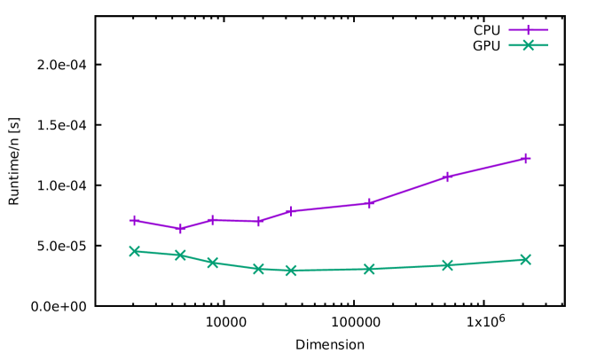
Figure 8 shows the runtime in seconds per degree of freedom for setting up the GCA-$\mathcal{H}^{2}$ matrix for different meshes approximating the unit sphere. For the CPU, we use an Intel Core i7-7820 with 8 cores and AVX 512 running at a base frequency of $3.6$ GHz, providing a peak performance of $460$ GFlops/s at double precision. For the GPU, we have used an AMD Vega 64 card running at 1.25 GHz with 8 GBytes of HBM2 memory and $4\,096$ arithmetic units providing a peak performance of 791 GFlops/s at double precision (and considerably more for single precision). It should be pointed out that this GPU is designed for the consumer market, so its double-precision performance is quite low. GPUs designed for computation like the NVIDIA Tesla P100 or V100 should provide around $5\,000$ and $7\,000$ GFlops/s at double precision, respectively.

Our figure suggests that both the CPU and the GPU implementation have $\mathcal{O}(n\log n)$ complexity: we use a logarithmic scale for the dimension $n$ and a linear scale for the work per degree of freedom, and the figure shows the latter as, essentially, a line. We can also see that the slope of this line for the CPU implementation is significantly steeper than for the GPU implementation. This suggests that the GPU implementation may become increasingly more attractive for larger meshes.

References

- [1] M. Bebendorf. Approximation of boundary element matrices. Numer. Math., 86(4):565–589, 2000.
- [2] M. Bebendorf and S. Rjasanow. Adaptive Low-Rank Approximation of Collocation Matrices. Computing, 70(1):1–24, 2003.
- [3] S. Börm. Efficient Numerical Methods for Non-local Operators: -Matrix Compression, Algorithms and Analysis, volume 14 of EMS Tracts in Mathematics. EMS, 2010.
- [4] S. Börm and S. Christophersen. Approximation of integral operators by Green quadrature and nested cross approximation. Numer. Math., 133(3):409–442, 2016.
- [5] S. Börm and L. Grasedyck. Low-rank approximation of integral operators by interpolation. Computing, 72:325–332, 2004.
- [6] S. Börm and L. Grasedyck. Hybrid cross approximation of integral operators. Numer. Math., 101:221–249, 2005.
- [7] S. Börm and W. Hackbusch. Data-sparse approximation by adaptive -matrices. Computing, 69:1–35, 2002.
- [8] S. Börm, M. Löhndorf, and J. M. Melenk. Approximation of integral operators by variable-order interpolation. Numer. Math., 99(4):605–643, 2005.
- [9] S. Chandrasekaran and I. C. F. Ipsen. On rank-revealing factorisations. SIAM J. Matrix Anal. Appl., 15(2):592–622, 1994.
- [10] Z. Gimbutas and V. Rokhlin. A generalized fast multipole method for nonoscillatory kernels. SIAM J. Sci. Comput., 24(3):796–817, 2002.
- [11] L. Greengard and V. Rokhlin. A new version of the fast multipole method for the Laplace equation in three dimensions. In Acta Numerica 1997, pages 229–269. Cambridge University Press, 1997.
- [12] W. Hackbusch, B. N. Khoromskij, and S. A. Sauter. On -matrices. In H. Bungartz, R. Hoppe, and C. Zenger, editors, Lectures on Applied Mathematics, pages 9–29. Springer-Verlag, Berlin, 2000.
- [13] W. Hackbusch and Z. P. Nowak. On the fast matrix multiplication in the boundary element method by panel clustering. Numer. Math., 54(4):463–491, 1989.
- [14] V. Rokhlin. Rapid solution of integral equations of classical potential theory. J. Comp. Phys., 60:187–207, 1985.
- [15] S. A. Sauter. Cubature techniques for 3-d Galerkin BEM. In W. Hackbusch and G. Wittum, editors, Boundary Elements: Implementation and Analysis of Advanced Algorithms, pages 29–44. Vieweg-Verlag, 1996.
- [16] S. A. Sauter and C. Schwab. Boundary Element Methods. Springer, 2011.
- [17] E. E. Tyrtyshnikov. Mosaic-skeleton approximation. Calcolo, 33:47–57, 1996.
- [18] L. Ying, G. Biros, and D. Zorin. A kernel-independent adaptive fast multipole algorithm in two and three dimensions. J. Comp. Phys., 196(2):591–626, 2004.