Power and Efficiency of a Thermal Engine with a Coherent Bath
Abstract
We consider a quantum engine driven by repeated weak interactions with a heat bath of identical three-level atoms. This model was first introduced by Scully et al. [Science, 2003], who showed that coherence between the energy-degenerate ground states serves as a thermodynamic resource that allows operation of a thermal cycle with a coherence-dependent thermalisation temperature. We consider a similar engine out of the quasistatic limit and find that the ground-state coherence also determines the rate of thermalisation, therefore increasing the output power and the engine efficiency only when the thermalisation temperature is reduced; revealing a more nuanced perspective of coherence as a resource. This allows us to optimise the output power by adjusting the coherence and relative stroke durations.
I Introduction
Quantum thermodynamics is concerned with how manifestly qfuantum phenomena, such as coherence and entanglement, affect thermal processes. A primary objective Goold et al. (2016); Vinjanampathy and Anders (2016) is understanding how these quantum phenomena can be harnessed to improve thermal processes, for example to increase work extraction from a heat engine. Conversely, what limitations does quantum mechanics place on thermal processes? There has been research investigating the work extracted from a quantum measurement Erez (2012); Kammerlander and Anders (2016); Jacobs (2012); Ding et al. (2018); Yi et al. (2017), or measurements with feedback (Funo et al., 2013; Maruyama et al., 2009; Elouard et al., 2017; Elouard and Jordan, 2018), known as a Maxwell’s demon. Systems initialised in non-equilibrium states allow for more work extraction according to generalisations of the second law Hasegawa et al. (2010); Niedenzu et al. (2018). Correlations between systems can also increase the extractable work Oppenheim et al. (2002); Perarnau-Llobet et al. (2015); Zurek (2003); Jevtic et al. (2012); del Rio et al. (2011), and there is a thermodynamic cost to creating correlations in uncorrelated, thermal systems Esposito et al. (2010).
Of particular interest is the effect of coherence in thermal processes. Although it contributes to the free energy, coherence cannot be extracted as work using thermal operations Lostaglio et al. (2015a); Korzekwa et al. (2016), but can be used as a catalyst Åberg (2014) and thought of as a quantum resource Baumgratz et al. (2014); Lostaglio et al. (2015b); Marvian et al. (2016). Instead of considering coherence in the system itself Scully et al. Scully et al. (2003) studied a system which interacted with a coherent heat bath. Specifically they considered a photo-Carnot engine — a single mode cavity undergoing a Carnot cycle — in which a heat bath is emulated by repeated weak interactions with identical three-level atoms with two degenerate ground states. Coherence between the two ground states can change the thermalisation temperature of the cavity, so a Carnot cycle can be implemented using a single bath and switching on coherence. There has been extensions to this setup, including adding cavity leakage Quan et al. (2006) and using entangled qubits Dillenschneider and Lutz (2009), or more general multi-atom baths Türkpençe et al. (2017); Dağ et al. (2016, 2019); Hardal and Müstecaplıoğlu (2015).
In the quasistatic limit, the efficiency is maximal, but since this requires infinite cycle duration, the output power is zero and the engine is impractical; one must trade off engine efficiency for output power Curzon and Ahlborn (1975). We investigate the effect on the power and efficiency of a quantum harmonic oscillator undergoing an Otto cycle with a coherent heat bath. Following Scully et al. we emulate a heat bath using repeated weak interactions with identical three-level systems with thermal populations and coherence between the two degenerate energy ground states. The interaction between the three-level atoms and the system is governed by a Jaynes-Cummings Hamiltonian, from which we derive a master equation for the state of the system. This allows us to analyse the performance of the engine in a more practical regime; without requiring the duration of each stroke to be infinite.
The two isentropic strokes involve changing the harmonic frequency . If this occurs rapidly then many off-diagonal coherences will be excited in the system. To correct for this effect we use shortcut-to-adiabaticity techniques (see Torrontegui et al. (2013) for a review). These techniques allow the state to undergo effectively adiabatic evolution in a finite time, and can be used to drive a thermal engine del Campo et al. (2014); Beau et al. (2016); Abah and Paternostro (2019); Abah and Lutz (2018). In Abah and Lutz (2017), the authors calculate a cost which must be paid to perform their shortcut-to-adiabaticity protocol, which increases with shorter stroke times. We adopt this cost as the reduction in work extracted during the Otto cycle.
This paper has the following structure. In section II we describe the interaction between the bath and the system, showing the change in the thermalisation temperature of the system when there is coherence between the ground states of the atoms. In section III we describe the four strokes of the Otto cycle, and in section IV we describe some issues with running an engine in finite time. Section V contains our results of the effect of coherence on the power and efficiency of the heat engine in the finite time regime; and in section VI we optimise the output power of the heat engine using coherence and by changing the relative duration of each stroke.
II Interaction with Bath
The working fluid of the heat engine is a quantum harmonic oscillator with unit mass, described by the Hamiltonian
| (1) |
where is the usual photon number operator. A sequence of -level atoms interact for a short time with the system, and after many weak interactions this stream of atoms emulates a thermal bath as it causes the system to thermalise. Here we leave the number of atomic energy levels general, but we will shortly assume that . The atoms have degenerate ground states and a single excited state with an energy level spacing tuned to the system frequency ,
| (2) |
In this paper we consider loss to the environment to be negligible and focus on the interaction with the atoms as the dominant process.
The interaction between a single atom and the system is described by the familiar Hamiltonian in the rotating wave approximation
| (3) |
where is the interaction strength. Introducing and , where , we can write the interaction Hamiltonian as . In the interaction picture with zero detuning, the total Hamiltonian reduces simply to the interaction Hamiltonian . Thus the interaction with duration is governed by the unitary
where we have expanded to second order in which is assumed to be small.
Assuming the atom starts in the initial state at some time , each interaction induces a completely positive trace preserving (CPTP) map on the system-atom product state :
| (4) | |||
where is the Lindblad superoperator. In the derivation of (4) we assumed that the atoms were block-diagonal in the energy basis, consequently
| (5) |
which removes the term of order . It is straightforward to show that this map contains thermal states as fixed points.
To derive a master equation, we first note that since is assumed small, the map (4) is equivalent to applications of a weaker imaginary map of time duration :
Considering a single step of this weaker map we can go to the continuum limit
| (6) |
which yields a dissipative Lindblad master equation
| (7) |
where for simplification we have rescaled time to the dimensionless parameter .
If the initial state of the system is diagonal in photon number, the steady state of the master equation satisfies
| (8) |
where the labeling and has been introduced to simplify the expressions.
If the atoms are prepared in a thermal state at inverse temperature then
| (9) |
where
| (10) |
and the partition function is . In this case and , and the steady state of the master equation (7) is a thermal distribution at inverse temperature ,
| (11) |
So the atoms, despite being a rather structured interaction, are emulating a thermal bath at a fixed temperature to which the system thermalises. It can be shown that if the system begins in a thermal state, then it remains in a thermal state under the evolution of this master equation, equilibrating to a particular temperature in the steady state.
In a thermodynamic analysis we are less interested in the explicit density matrix, than the internal energy. Changes in average energy are proportional to changes in average photon number, . Master equation (7) allows us to derive a time evolution equation for the mean photon number ,
| (12) |
This equation has the solution
| (13) |
The steady state limit exists provided and is
| (14) |
If then the average photon number will increase unbounded and the system will not thermalise. While this can be achieved using coherence, the atoms cease to behave similarly to a thermal bath and so we exclude this case.
For simplicity, from here onwards we will use .
In the steady state limit, the harmonic oscillator is in a thermal state, and the steady state average photon number is related to the inverse temperature as
| (15) |
and therefore system will thermalise to the temperature
| (16) |
The temperature is strictly monotonic in , so we can consider as the effective temperature of the atoms. Hence in section V when we compare different pairs of thermal baths with the same effective temperatures, we are holding constant.
The value of (and hence and too) is altered by coherence in the energy ground space of the atoms. In general the atoms are block-diagonal in energy
| (17) |
where is defined as it was previously (10), and is the quantum state in the degenerate ground subspace. Hence . Coherence in the energy ground space can be chosen to increase or decrease the thermalisation temperature of the system
| (18) |
In the case of no coherence then and . Coherence can be used to make the effective temperature arbitrarily hot; as approaches from above, the thermalisation temperature tends to infinity. However since , the effective temperature can only be lowered as cold as
| (19) |
A corollary is that when using maximal coherence to lower the effective temperature of a thermal bath, the final temperature is bounded from above
| (20) |
It may seem paradoxical that the coherence in the ground state can raise the thermalisation temperature of the system arbitrarily; however, this is not a mysterious consequence of quantum coherence but simply due to the nature of the coupling between the atoms and field (3). By tuning the quantum state in the ground subspace we can prevent the system from releasing energy to the atoms and so each interaction can only increase the energy of the system.
For the rest of this paper we will specialise to the case in which .
III The Otto cycle
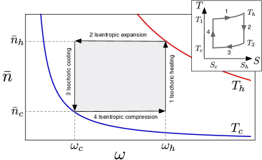
In this section we examine the heat engine under the quasistatic evolution of the Otto thermal cycle. The Otto cycle (see FIG. 1) involves the following four strokes:
-
1.
Isochoric heating: the system interacts with the hot bath, eventually thermalising to temperature .
-
2.
Isentropic expansion: the system is isolated from the heat baths and the system frequency is decreased . Work is extracted from the system.
-
3.
Isochoric cooling: the system interacts with the cold bath, eventually thermalising to temperature .
-
4.
Isentropic compression: the system is isolated from the heat baths and the system frequency is increased . Work is performed on the system to close the cycle.
The Otto cycle allows the easy quantification of heat and work for a cycle. Since the isochoric (constant volume) stokes involve no change of the system Hamiltonian, any change in energy is due to a heat flow between the system and thermal baths, . During the isentropic (constant entropy) strokes, the system is isolated, and so any change in energy is due to work done on the system, . Compare this to the Carnot cycle, where work is done on the system during every stroke. The internal energy is and hence
| (21) |
which is a statement of the first law for this system. During a quasi-static evolution the system remains in a thermal state. The entropy can be found by integrating
| (22) |
from which we find
| (23) |
The efficiency of the Otto cycle is the ratio of the work extracted to the heat input from the hot bath
| (24) |
We can easily read off from FIG. 1 that the work done in a cycle is the area , and therefore
| (25) |
We can relate this to the temperature (see FIG. 1), since during the work strokes, the product is constant,
| (26) |
IV The Finite Time Regime
Previous works Scully et al. (2003); Quan et al. (2006); Dillenschneider and Lutz (2009); Türkpençe and Müstecaplıoğlu (2016) have considered a harmonic oscillator undergoing a Carnot or Otto cycle in the quasistatic limit. However the quasistatic limit is impractical as it produces zero output power; so we examine the harmonic oscillator undergoing a finite time Otto cycle. In this section we discuss two issues in operating a heat engine for finite time. During the work strokes, we use shortcut-to-adiabaticity techniques to control the system energy populations; and during the heat strokes, we need to guarantee that the average energy returns to its original value at the end of each cycle.
IV.1 Work Strokes
During the work strokes, the system evolves under the time-dependent Hamiltonian Abah and Lutz (2017); Deffner et al. (2010); Husimi (1953)
| (27) |
If the system frequency is changed very slowly, then by the adiabatic theorem, the state of the system is constant. Quickly changing the frequency will excite off-diagonal terms in the density matrix. Using shortcuts-to-adiabaticity (STA) techniques Torrontegui et al. (2013), the state of the system can be constant even when quickly changing the frequency (this has recently been demonstrated experimentally Deng et al. (2018); Diao et al. (2018)). This can be achieved by adding a counterdiabatic term to the Hamiltonian, . For example, in del Campo (2013), the author uses the following counterdiabatic term
| (28) |
The author changes the system frequency according to
| (29) |
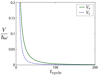
This protocol will change the frequency from in time . The author shows that if the system begins in a thermal state, then under this counterdiabatic Hamiltonian (28), the energy populations will be constant. Such a protocol can be used to drive an thermal cycle del Campo et al. (2014); Beau et al. (2016); Abah and Paternostro (2019); Abah and Lutz (2018); we use this protocol as well. The authors in Abah and Lutz (2017) describe an energy cost associated with the addition of this counterdiabatic term, given by
| (30) |
where is the average photon number at ; which implies the isentropic expansion strokes will have a larger energy cost than the compression strokes (see FIG. 2; in all our plots, the integration was completed numerically). The energy cost is monotonically decreasing in the stroke duration. We note here that while we adopt the energy cost described in Abah and Lutz (2017), there exists a diversity of opinion about what constitutes the appropriate energy cost of running a shortcut-to-adiabaticity protocol Abah and Paternostro (2019); Kosloff and Rezek (2017); Torrontegui et al. (2017); Zheng et al. (2016); Calzetta (2018).
The efficiency of the heat engine will therefore be diminished by two energy costs and , one each for the isentropic expansion and compression strokes
| (31) |
The authors of Abah and Lutz (2017) consider the cost as an additional heat input into the system. We disagree with this. This energy cost is due to a unitary process when the system is isolated from other systems. Therefore we consider the energy cost as a reduction in the work extracted from the system.
Using this counterdiabatic term the energy populations of the system are constant, and therefore the average photon number of the system is constant. We assume that the change in energy of the system during the isentropic expansion stroke is entirely extracted as work. Hence, the net extracted work is proportional to the change in the frequency of the system .
IV.2 Heat Strokes
During the heating (isochoric) strokes, the system frequency is constant, and the heat into the system is proportional to the change in the average photon number of the system.
We assume the system begins in a thermal state. After a single cycle, the system has interacted with the hot bath for time , and the cold bath for time . If the systems begins with an arbitrary initial average photon number , it is not guaranteed that the cycle will be closed, since may not return to its initial value. In this section we show that the system will always asymptotically approach a “steady cycle”, where the average photon number at the end of the cycle is the same as that at the beginning of the cycle.
Since is constant during the work strokes, the average photon number after one cycle is given by two applications of (13),
| (32) |
Recall that we defined , the difference in the transition rates of the master equation (7). We have introduced subscripts and to denote the terms which arise due to interactions with the hot and cold baths respectively. We want to know the initial photon number such that . We denote it ,
| (33) |
If the interaction time with the cold bath is large, then is the thermalisation average photon number of the cold bath.
| (34) |
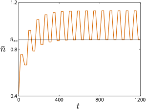
So if the system begins with , then after one cycle, the average photon number will return to . However even if , after multiple cycles the the average photon number at the beginning of a cycle will tend to . After cycles (see Appendix A for details)
| (35) |
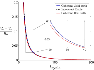
so, as seen in FIG. 3,
| (36) |
and the system always reaches a ‘steady cycle’, where the average photon number returns to its initial value after each cycle. This has been previously studied in Feldmann et al. (1996); Kosloff and Rezek (2017). We assume for the rest of this paper that the system has reached a steady cycle.
V Performance
V.1 The effect of coherence
The work extracted in a single cycle is . We can use (13) to write
| (37) |
where the average photon number begins from and evolves to . In a steady cycle, is given by (33), and so
| (38) |
Keeping the temperature of the baths constant, is monotonically increasing in both and (see Appendix B.1, for the calculation).
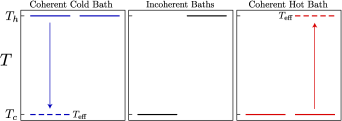
We have seen that coherence in the energy ground space of the incoming atoms can increase or decrease the effective temperature of atomic thermal bath (see section II). To investigate the effect of coherence on the power of the engine, we study three pairs (hot and cold) of heat baths, all at the same effective inverse temperatures, and . The first is a pair of incoherent (I) baths, with thermalisation photon numbers
| (39) |
| Incoherent Baths (I) | ||||
|---|---|---|---|---|
| Coherent Hot Bath (CH) | ||||
| Coherent Cold Bath (CC) |
We compare this with two other pairs of baths with the same effective temperatures. The first pair (coherent hot or CH) have cold thermal populations consistent with inverse temperature , however there is coherence in the energy ground space of one of the baths such that the effective inverse temperature is that of the incoherent hot bath . Explicitly
| (40) |
The second pair of thermal baths (coherent cold or CC) is the reverse: hot thermal populations at inverse temperature , but with sufficient coherence in the ground space of one of the bath such that it has an effective inverse temperature of the incoherent cold bath . That is
| (41) |
These three different pairs of baths are summarised in FIG. 4. Without the addition of coherence, these latter two pairs of baths would be unusable; the addition of coherence creates an effective temperature difference, and allows them to be used to extract work, as seen in Scully et al. (2003). In the first case the coherence is being used to turn a cold bath into a hot bath, and in the second case coherence is being used to change a hot bath into a cold bath. We note here that
| (42) |
From (13), effects not only the effective temperature of the bath but also the rate at which the system thermalises. Faster thermalisation allows more work to be extracted per cycle. Creating the coherent hot bath requires a smaller as compared with the incoherent bath pair, and less work will be extracted in a cycle. Conversely, the creation of the coherent cold bath requires a larger than the incoherent baths, and more work will be extracted per cycle.
V.2 Cost
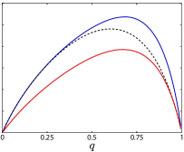
The cost of the shortcut-to-adiabaticity protocol (30) is proportional to the average photon number of the system at the beginning of the protocol. This will be different for the different bath systems, since this depends not only on the temperature of the baths but also on the thermalisation rates and . The cost of the compression stroke is proportional to the average photon number . Since we are assuming the system has reached a steady cycle, this is given by (33). If we keep the temperature of the baths constant but change the absorption rate and , we can see that is monotonically increasing in , but monotonically decreasing in . This is also true for the expansion stroke cost , during which the average photon number is (see Appendix B.2 for details).
This implies, from (42) that the use of coherence either to increase the temperature of a hot bath, or to decrease the temperature of a cold bath, both reduce the cost of the shortcut-to-adiabaticity protocol. As can be seen in FIG. 5, the CC and CH bath systems using coherence have a smaller energy cost than the incoherent (I) bath system.
V.3 Efficiency
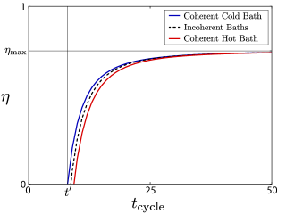
The efficiency (31) is reduced from maximum because of the cost of implementing the shortcut-to-adiabaticity protocol.
| (43) |
Since the cost tends toward zero with increasing cycle time , engines in which the expansion and compression strokes have a longer duration will be more efficient (as shown in FIG. 6). There is a time , before which, the energy cost of the shortcut-to-adiabaticity protocol will exceed the work extracted. This will result in a negative efficiency, rendering the engine too expensive to run.
For the baths that we have hitherto examined, coherence has reduced the cost of the shortcut-to-adiabaticity protocol. However the reduction in the efficiency is also inversely dependent upon the heat input to the system by the hot bath , which is proportional to (38). We saw previously that is monotonically increasing in both and (see Appendix B.1). In the case of the CC thermal baths the thermalisation rate , so the heat input from the hot bath , is greater than the heat input using incoherent thermal baths ,
| (44) |
We can immediately deduce an improvement in the efficiency using the CC thermal baths. Since the CC thermal baths have a smaller shortcut-to-adiabaticity energy cost and a larger heat input , then from (43) we must have
| (45) |
For the CH thermal baths, the coherence provides a reduction in the cost of the shortcut-to-adiabaticity protocol, however since , there is a reduction in the heat input to the system
| (46) |
It can be shown (see Appendix B.3 for details) that the reduction in heat into the system outweighs the benefit of coherence in reducing the cost of the shortcut-to-adiabaticity protocol, and we have (see FIG. 6)
| (47) |
V.4 Power
The power generated from a single thermal cycle (of duration ) is the work per unit time
| (48) |
The work extracted is . Using (38), we can rewrite the power as
| (49) |
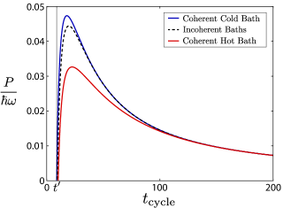
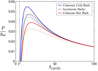
FIG. 7 compares for the different thermal baths. As we saw in the previous section, before time the cost is greater than the work extracted, and the engine becomes too costly to run. As , the work approaches a constant value
| (50) |
and . Since is the product of transcendental functions, we cannot find an analytic expression for the cycle time at which is maximal.
To reiterate, the work is proportional to which is monotonic in and (see Appendix B.1). Since , the work extracted from the CC baths in a cycle is greater than the incoherent (I) baths.
The CC baths extract more work, and have a smaller shortcut-to-adiabaticity energy cost, so we can immediately deduce an increase in power (FIG. 7)
| (51) |
The CH baths also have a smaller energy cost, however , which implies that less work is extracted in a cycle from the CH baths than the incoherent (I) baths. The power of the CH baths need not be less than the incoherent baths (I), but in our simulations we find it typically is (see Appendix B.4 for details). In FIG. 7, the decrease in work extracted in a single cycle is large enough such that there is a net decrease in the power of the CH baths, i.e. .
VI Optimising the Power
VI.1 Using coherence
Can we further improve the output power? So far we have been looking at two extremes: using coherence to generate a hot bath (CH) and a cold bath (CC), with the other bath in each pair having no coherence (refer to FIG. 4). But what about in-between these two extremes? We could compare these baths with others in which both hot and cold baths are created using coherence. We could look at the continuum in between these two extremes, parametrised by :
| (52) | ||||
where . The limiting cases are those studied in the previous section: corresponds to the CH baths and corresponds to the CC baths. Along this continuum, the maximal work per cycle is achieved at . In the previous section we mentioned numerous times (shown in Appendix B.1) that the work extracted in a single cycle is monotonically increasing with and . Since , we see that and are maximised when . Using coherence to decrease the temperature of a bath increases the work extracted per cycle, and using coherence to increase the temperature of a bath decreases the work extracted per cycle. Thus it is expected to be that the optimal bath combination would be to use coherence to cool the cold bath, and to use no coherence in heating the hot bath.
This reasoning suggests the way to maximise the work extracted per cycle using coherence is to create both the hot and cold baths from hotter baths, using as much coherence as possible to decrease their effective temperatures. However as we saw in section II, if a system is cooled maximally, then the effective temperature . Such a bath can be created using coherence to cool a thermal bath with temperature
| (53) |
A bath with temperature can be created by using coherence to cool a bath of infinite temperature.
VI.2 Changing stroke times
Hitherto, we have been assuming that for a given cycle time , each stroke had equal duration . The system interacts with the heat baths for a total time , and work is done on the system for a time . We can break down further, as , where is the duration of the isentropic expansion, and is the duration of the isentropic compression.
We can improve the output power of the heat engine by altering all the relative times of the four cycle strokes. We parametrise this using three variables.
First, we can alter the relative durations of the heat and work strokes within a single cycle. We parametrise the total cycle time as follows
| (54) |
Increasing the proportion of in which the system interacts with the heat bath causes more heat to flow in and out of the system, allowing more work to be extracted per cycle, at the price of a larger energy cost in running the shortcut-to-adiabaticity protocol. We want to find the value of in which the peak power is maximised. We cannot find an analytic expression for an optimal value for , so we proceed numerically.
We can further parametrise and ,
| (55) |
Increasing the proportion of which the system interacts with the hot bath allows more heat to enter the system, increasing the work that can be extracted. However less heat is transferred to the cold bath, so more work is required during the compression stroke. The costs of expansion () and compression () differ due to the different initial average photon numbers (see FIG. 2). Increasing reduces the cost of the isentropic expansion strokes; however, it increases the cost of the isentropic compression strokes.
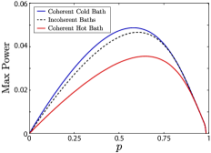
We want to find the values of such that the peak power is maximised. That is, we want to maximise the following function
| (56) |
In FIG. 8, three cross sections of this function are shown, one for each variable. We see the values which maximise the power are different for each of the baths. We numerically found values of which maximised the Max Power for the CC baths with arbitrarily chosen temperatures. In this case we found a bias towards increasing the duration of the heat strokes over the work strokes, and in particular a higher proportion of the interaction time to be with the hot bath. The power is also improved by slightly slowing the expansion strokes. In FIG. 9 the improvement in the power curve with these values is shown.
VII Conclusion
Coherence in the energy ground space of the atoms used to emulate a thermal bath does not change the average energy of the atoms, but changes the interaction of the atoms with the system; specifically the rate at which the system loses photons to the incoming atoms. This has two effects. First, it changes the thermalisation temperature of the system. So coherence can be used to create a temperature difference in two baths which previously were in equilibrium. Secondly, it changes the rate of thermalisation . These effects are inversely correlated, in that decreasing the thermalisation temperature causes an increase in the rate of thermalisation, and vice versa. In this paper we have shown how the coherence can be used to increase (or decrease) the power and efficiency of a heat engine. We used coherence to create a temperature difference between two bath systems in equilibrium; creating both a cold bath, and a hot bath. In both cases, the coherence reduced the cost of implementing the shortcut-to-adiabaticity protocol. Using coherence to create the cold bath improved the power of the engine, because it increased the thermalisation rate , allowing more heat transfer into the system in a cycle, and more work to be extracted. The efficiency was also improved, because the increased heat into the system reduced the effect of the cost of the shortcut-to-adiabaticity protocol. Conversely, creating a hot bath requires the thermalisation rate to be reduced, which can in turn reduce the output power of the engine, and always reduces the efficiency. This demonstrates a more nuanced and subtle perspective of the benefit of coherence in the finite-time regime, it is a quantity which requires careful optimisation. The output power can be further improved by using the maximum amount of coherence in cooling the heat baths, also by changing the relative durations of the four strokes in the thermal cycle.
This work can be extended by considering a quantum trajectory unravelling of the master equation (7). This would involve continuously monitoring the photon number of the system, and using that information to reduce the duration of the heat strokes. Of course the memory which stores the measurement results would need to be erased to close the cycle. Considering atoms with a larger number of degenerate ground states, might allow more efficient energy transfer between the bath and system. Furthermore, correlated states between the atoms would allow the study of more general quantum resources, extending beyond Markovian interactions.
Acknowledgements.
T. Guff would like to thank J. D. Cresser for his many useful conversations. This research was funded in part by the Australian Research Council Centre of Excellence for Engineered Quantum Systems (Project number CE110001013, CE170100009).Appendix A Steady Cycle
After driving the heat engine through Otto cycles, using the shortcut-to-adiabaticity techniques during the work strokes, the average photon number is (32)
| (57) |
where is the average photon number at the end of cycles. If we recursively expand this using (13) until we reach the initial photon number , we find (with some algebra)
| (58) |
From (33) we can identify
| (59) |
Further we can identify the geometric series
| (60) |
We combine these to rewrite (58) as
| (61) |
Appendix B Derivatives
B.1 Work
The work is proportional to the change in the average photon number, , which is given by (38). With the bath temperatures held constant, this function is monotonically increasing in and . We see this by calculating derivatives,
| (62a) | ||||
| (62b) | ||||
where
| (63a) | ||||
| (63b) | ||||
So both derivatives in (62) are both positive. Therefore more work is extracted per cycle by increasing and .
B.2 Cost
The cost of implementing the shortcut-to-adiabaticity protocol depends on the thermal baths in that it is proportional to the initial average photon number (30). At the beginning of the compression strokes, the initial photon number is given by the steady cycle initial photon number (33). By calculating the derivatives of this function, holding the temperature of the baths constant, we find
| (64a) | ||||
| (64b) | ||||
where
| (65a) | ||||
| (65b) | ||||
so is monotonically increasing in , but monotonically decreasing in . The expansion strokes begin after the system has interacted with the hot bath for a time . That is, the system begins with , and then evolves under (13) for time , interacting with the hot bath, after which the average photon number is
| (66) |
If the interaction time with the hot bath is large, then the the average photon number is the thermalisation photon number of the hot bath
| (67) |
Once again taking derivatives we find
| (68a) | ||||
| (68b) | ||||
where
| (69a) | ||||
| (69b) | ||||
and likewise, is monotonically increasing in , but monotonically decreasing in .
B.3 Efficiency
The efficiency (31) is reduced from maximum by the cost of implementing the shortcut-to-adiabaticity protocol, over the heat input into the system. The work costs and are proportional to the average photon number of the system at the beginning of the expansion and compression. Therefore we can write and , where (as can be seen in (30)), and are integrals which are independent of the choice of bath.
The CC baths have a smaller energy cost, and a larger heat input per cycle than the incoherent (I) baths: therefore the efficiency of the CC baths is always greater. However, the CH baths have a smaller shortcut-to-adiabaticity energy cost compared with the incoherent (I) baths, but also a smaller heat input . To see the effect on the efficiency in using the CH baths, we need to compare
| (70) |
Using (33), (38), and (66), we have
| (71a) | ||||
| (71b) | ||||
The difference between and is constant. We want the derivative with respect to , keeping the temperature of the hot bath constant.
| (72) |
so and are monotonically decreasing with . Changing from the I thermal baths to the CH thermal baths involves decreasing , which increases and . Thus we have
| (73) |
So
| (74) |
and hence
| (75) |
B.4 Power
The CC baths extract more work per cycle than the incoherent (I) baths, and also have a smaller shortcut-to-adiabaticity energy cost. Hence the output power of the CC is always larger than the incoherent (I) baths.
However, the work extracted in a single cycle using the CH baths is less than the I baths, and the use of coherence means there is a smaller shortcut-to-adiabaticity cost, .
The output power of the thermal engine is given by (49)
As in the previous section we can rewrite the energy cost
| (76) |
where is given by (66) and is given by (33). We want to know whether the power of the CH baths is strictly less than the incoherent (I) baths. So we want the derivative of with respect to , keeping temperature constant.
| (77) |
The power is monotonically increasing in if
| (78) |
If the difference in system frequencies is large compared with the energy costs , then will be monotonically increasing, and the power of the CH baths will be less than that of the incoherent (I) baths. However, if and , then will be monotonically decreasing for all but large values of , and the power CH baths will exceed that of the incoherent (I) baths.
References
- Goold et al. (2016) J. Goold, M. Huber, A. Riera, L. d. Rio, and P. Skrzypczyk, J. Phys. A 49, 143001 (2016).
- Vinjanampathy and Anders (2016) S. Vinjanampathy and J. Anders, Contemp. Phys. 57, 545 (2016).
- Erez (2012) N. Erez, Phys. Script. T151, 014028 (2012).
- Kammerlander and Anders (2016) P. Kammerlander and J. Anders, Sci. Rep. 6, 22174 (2016).
- Jacobs (2012) K. Jacobs, Phys. Rev. E 86, 040106 (2012).
- Ding et al. (2018) X. Ding, J. Yi, Y. W. Kim, and P. Talkner, Phys. Rev. E 98, 042122 (2018).
- Yi et al. (2017) J. Yi, P. Talkner, and Y. W. Kim, Phys. Rev. E 96, 022108 (2017).
- Funo et al. (2013) K. Funo, Y. Watanabe, and M. Ueda, Phys. Rev. A 88, 052319 (2013).
- Maruyama et al. (2009) K. Maruyama, F. Nori, and V. Vedral, Rev. Mod. Phys. 81, 1 (2009).
- Elouard et al. (2017) C. Elouard, D. Herrera-Martí, B. Huard, and A. Auffèves, Phys. Rev. Lett. 118, 260603 (2017).
- Elouard and Jordan (2018) C. Elouard and A. N. Jordan, Phys. Rev. Lett. 120, 260601 (2018).
- Hasegawa et al. (2010) H.-H. Hasegawa, J. Ishikawa, K. Takara, and D. Driebe, Phys. Lett. A 374, 1001 (2010).
- Niedenzu et al. (2018) W. Niedenzu, V. Mukherjee, A. Ghosh, A. G. Kofman, and G. Kurizki, Nat. Comms. 9, 165 (2018).
- Oppenheim et al. (2002) J. Oppenheim, M. Horodecki, P. Horodecki, and R. Horodecki, Phys. Rev. Lett. 89, 180402 (2002).
- Perarnau-Llobet et al. (2015) M. Perarnau-Llobet, K. V. Hovhannisyan, M. Huber, P. Skrzypczyk, N. Brunner, and A. Acín, Phys. Rev. X 5, 041011 (2015).
- Zurek (2003) W. H. Zurek, Phys. Rev. A 67, 012320 (2003).
- Jevtic et al. (2012) S. Jevtic, D. Jennings, and T. Rudolph, Phys. Rev. Lett. 108, 110403 (2012).
- del Rio et al. (2011) L. del Rio, J. Åberg, R. Renner, O. Dahlsten, and V. Vedral, Nat. 474, 61 (2011).
- Esposito et al. (2010) M. Esposito, K. Lindenberg, and C. Van den Broeck, New J. Phys. 12, 013013 (2010).
- Lostaglio et al. (2015a) M. Lostaglio, D. Jennings, and T. Rudolph, Nat. Comms. 6, 6383 (2015a).
- Korzekwa et al. (2016) K. Korzekwa, M. Lostaglio, J. Oppenheim, and D. Jennings, New J. Phys. 18, 023045 (2016).
- Åberg (2014) J. Åberg, Phys. Rev. Lett. 113, 150402 (2014).
- Baumgratz et al. (2014) T. Baumgratz, M. Cramer, and M. B. Plenio, Phys. Rev. Lett. 113, 140401 (2014).
- Lostaglio et al. (2015b) M. Lostaglio, K. Korzekwa, D. Jennings, and T. Rudolph, Phys. Rev. X 5, 021001 (2015b).
- Marvian et al. (2016) I. Marvian, R. W. Spekkens, and P. Zanardi, Phys. Rev. A 93, 052331 (2016).
- Scully et al. (2003) M. O. Scully, M. S. Zubairy, G. S. Agarwal, and H. Walther, Sci. 299, 862 (2003).
- Quan et al. (2006) H. T. Quan, P. Zhang, and C. P. Sun, Phys. Rev. E 73, 036122 (2006).
- Dillenschneider and Lutz (2009) R. Dillenschneider and E. Lutz, EPL 88, 50003 (2009).
- Türkpençe et al. (2017) D. Türkpençe, F. Altintas, M. Paternostro, and Ö. E. Müstecaplıoğlu, EPL 117, 50002 (2017).
- Dağ et al. (2016) C. B. Dağ, W. Niedenzu, Ö. E. Müstecaplıoğlu, and G. Kurizki, Ent. 18, 244 (2016).
- Dağ et al. (2019) C. B. Dağ, W. Niedenzu, F. Ozaydin, Ö. E. Müstecaplıoğlu, and G. Kurizki, J. Phys. Chem. C 123, 4035 (2019).
- Hardal and Müstecaplıoğlu (2015) A. Ü. C. Hardal and Ö. E. Müstecaplıoğlu, Sci. Rep. 5, 12953 (2015).
- Curzon and Ahlborn (1975) F. L. Curzon and B. Ahlborn, Am. J. Phys. 43, 22 (1975).
- Torrontegui et al. (2013) E. Torrontegui et al., Adv. Atom. Mol. Opt. Phys. 62, 107 (2013).
- del Campo et al. (2014) A. del Campo, J. Goold, and M. Paternostro, Sci. Rep. 4, 6208 (2014).
- Beau et al. (2016) M. Beau, J. Jaramillo, A. del Campo, M. Beau, J. Jaramillo, and A. del Campo, Ent. 18, 168 (2016).
- Abah and Paternostro (2019) O. Abah and M. Paternostro, Phys. Rev. E 99, 022110 (2019).
- Abah and Lutz (2018) O. Abah and E. Lutz, Phys. Rev. E 98, 032121 (2018).
- Abah and Lutz (2017) O. Abah and E. Lutz, EPL 118, 40005 (2017).
- Türkpençe and Müstecaplıoğlu (2016) D. Türkpençe and Ö. E. Müstecaplıoğlu, Phys. Rev. E 93, 012145 (2016).
- Deffner et al. (2010) S. Deffner, O. Abah, and E. Lutz, Chem. Phys. 375, 200 (2010).
- Husimi (1953) K. Husimi, Prog. T. Phys. 9, 381 (1953).
- Deng et al. (2018) S. Deng, A. Chenu, P. Diao, F. Li, S. Yu, I. Coulamy, A. del Campo, and H. Wu, Sci. Adv. 4, eaar5909 (2018).
- Diao et al. (2018) P. Diao, S. Deng, F. Li, S. Yu, A. Chenu, A. del Campo, and H. Wu, New J. Phys. 20, 105004 (2018).
- del Campo (2013) A. del Campo, Phys. Rev. Lett. 111, 100502 (2013).
- Kosloff and Rezek (2017) R. Kosloff and Y. Rezek, Entropy 19, 136 (2017).
- Torrontegui et al. (2017) E. Torrontegui, I. Lizuain, S. González-Resines, A. Tobalina, A. Ruschhaupt, R. Kosloff, and J. G. Muga, Physical Review A 96, 022133 (2017).
- Zheng et al. (2016) Y. Zheng, S. Campbell, G. De Chiara, and D. Poletti, Physical Review A 94, 042132 (2016).
- Calzetta (2018) E. Calzetta, Physical Review A 98, 032107 (2018).
- Feldmann et al. (1996) T. Feldmann, E. Geva, R. Kosloff, and P. Salamon, Am. J. Phys. 64, 485 (1996).