Stochastic Primal-Dual Q-Learning

Abstract

In this work, we present a new model-free and off-policy reinforcement learning (RL) algorithm, that is capable of finding a near-optimal policy with state-action observations from arbitrary behavior policies. Our algorithm, called the stochastic primal-dual Q-learning (SPD Q-learning), hinges upon a new linear programming formulation and a dual perspective of the standard Q-learning. In contrast to previous primal-dual RL algorithms, the SPD Q-learning includes a Q-function estimation step, thus allowing to recover an approximate policy from the primal solution as well as the dual solution. We prove a first-of-its-kind result that the SPD Q-learning guarantees a certain convergence rate, even when the state-action distribution is time-varying but sub-linearly converges to a stationary distribution. Numerical experiments are provided to demonstrate the off-policy learning abilities of the proposed algorithm in comparison to the standard Q-learning.

Keywords: Reinforcement learning (RL), Saddle point problem, Markov decision process (MDP), Q-learning

1 Introduction

The problem of learning a map from world observations to actions, called a policy, lies at the core of many sequential decision problems, such as robotics (Chen et al., 2017), artificial intelligence (Mnih et al., 2015), finance (Longstaff and Schwartz, 2001), and economics (Tesauro and Kephart, 2002). The development of policies is often very challenging in many real-world applications as finding accurate world models is difficult under complex interactions between the decision maker and environment. Reinforcement learning (RL) (Sutton and Barto, 1998; Bertsekas and Tsitsiklis, 1996; Puterman, 2014) is a subfield of machine learning which addresses the problem of how an autonomous agent (decision maker) can learn an optimal policy to maximize long-term cumulative rewards, while interacting with unknown environment.

Many classical RL algorithms, e.g., temporal difference methods (Sutton, 1988), Q-learning (Watkins and Dayan, 1992), SARSA (Rummery and Niranjan, 1994), are based on the sample-based stochastic dynamic programming to solve the Bellman equation, taking advantage of its contraction mapping property to guarantee their convergence. Comprehensive reviews of the dynamic programming and RL approaches can be found in the books Sutton and Barto (1998); Bertsekas and Tsitsiklis (1996); Puterman (2014). Recently, there has been a growing interest in integrating Bellman equations into optimization frameworks to design provably efficient RL algorithms, by leveraging the existing fruitful optimization algorithms and theories. See, e.g., Baird (1995); Sutton et al. (2009a); Mahadevan et al. (2014); Dai et al. (2017) for policy evaluation and Wang and Chen (2016); Chen and Wang (2016); Dai et al. (2018a, b) for policy design. In particular, Chen and Wang (2016) considers a linear programming form of the Bellman equation and introduces a stochastic primal-dual (SPD) algorithm to solve the min-max problem of the associated Lagrangian function, assuming samples from a uniform state-action distribution. The primal-dual optimization perspective is further employed in Dai et al. (2018a) with nonlinear function approximations to solve Markov decision problems with continuous state-actions spaces. Besides the direct advantage of theoretical guarantees, such optimization frameworks are also very favorable and extensible when dealing with constraints, sparsity regularizations (Mahadevan and Liu, 2012), and distributed scenarios (Kar et al., 2013; Macua et al., 2015; Zhang et al., 2018; Lee et al., 2018).

Statement of Contributions: Although substantial advances have been made recently in this direction, to the authors’ knowledge, finding a reliable suboptimal policy using samples from real-world trajectories remains largely unexplored, leaving a huge gap between theory and practice. Inspired by the above discussions, this paper centers at filling in this gap by proposing a new linear programming (LP) formulation of the standard Q-learning (Watkins and Dayan, 1992), known to be one of the most popular RL algorithms for policy design, in order to leverage its powerful model-free and off-policy learning abilities to solve Markov decision making problems. The main contributions are summarized below.

1. We develop a novel stochastic primal-dual Q-learning (SPD Q-learning) algorithm to solve the corresponding Lagrangian of the LP, that uses only samples of real-world trajectories without any importance sampling steps, as usually required in off-policy RL algorithms (Precup et al., 2001). The proposed algorithm includes a Q-function estimation step, and allows recovering an optimal policy using the primal solutions as well as the dual solutions.

2. Moreover, the SPD Q-learning is the first RL which guarantees the convergence with a certain convergence rate even when the underlying distribution of the state-action observations is time-varying but sub-linearly converges to a stationary distribution. This result applies to important cases, such as when the state distribution under a fixed behavior policy is time-varying, or when the behavior policy itself is time-varying.

3. We provide a detailed convergence and sample complexity analysis for the SPD Q-learning algorithm. In particular, we prove that with the number of iterations/samples at least ${\cal O}\left(\frac{|{\cal S}|^{4}|{\cal A}|^{4}}{\zeta^{4}(1-\alpha)^{4}}\frac{1}{\varepsilon^{2}}\ln\left(\frac{1}{\delta}\right)\right)$, the algorithm generates a candidate solution with duality gap less than or equal to $\varepsilon$ with probability $1-\delta$, where $|{\cal S}|$ is the number of the states, $|{\cal A}|$ is the number of the actions, $\alpha\in(0,1)$ is the discount factor, and $\zeta\in(0,1)$ is a constant related to the state-action distribution. This result also leads to the conclusion that with the number of iterations at least ${\cal O}\left(\frac{|{\cal S}|^{6}|{\cal A}|^{4}}{\zeta^{4}(1-\alpha)^{6}}\frac{1}{\varepsilon^{2}}\ln\left(\frac{1}{\delta}\right)\right)$, an $\varepsilon$-suboptimal policy can be recovered from the algorithm with probability at least $1-\delta$, where the policy is $\varepsilon$-suboptimal in the sense that the distance between the optimal value function and the value function corresponding to the obtained policy is less than or equal to $\varepsilon$.

4. To demonstrate the validity of the proposed algorithm, we provide simulation results for simple Markov decision making problems. Through the simulations, we observe that the suboptimal policy recovered from the primal solution converges faster than the suboptimal policy from the dual solution, and this is a potential advantage of the proposed algorithm.

We expect that this fundamental framework will be useful to advance many subfields of RL, such as the distributed RL (Kar et al., 2013; Macua et al., 2015; Zhang et al., 2018; Lee et al., 2018), Q-learning with function approximations (Sutton et al., 2009b, a), sparsity promoted RL (Mahadevan and Liu, 2012), safe RL (Garcıa and Fernández, 2015), and the inverse RL (Ng and Russell, 2000).

The remainder of the paper is organized as follows. Section 2 contains preliminaries including notations, definitions, problem formulations, standard LP formulation of the dynamic programming, and its solution analysis. Section 3 proposes a new LP formulation of the dynamic programming tailored to the proposed Q-learning algorithm, its solution analysis, and the main SPD Q-learning algorithm. The corresponding convergence results of the SPD Q-learning algorithm are summarized in Section 4, and detailed proofs are included in Section 5. Simulation results are given in Section 6, and finally, we provide conclusions in Section 7.

Notation: The following notation is adopted: ${\mathbb{R}}^{n}$ denotes the $n$-dimensional Euclidean space; ${\mathbb{R}}^{n\times m}$ denotes the set of all $n\times m$ real matrices; ${\mathbb{R}}_{+}^{n}$ and ${\mathbb{R}}_{++}^{n}$ denote the sets of vectors with nonnegative and positive real elements, respectively, $A^{T}$ denotes the transpose of matrix $A$; $I_{n}$ denotes the $n\times n$ identity matrix; $I$ denotes the identity matrix with appropriate dimension; $\|\cdot\|_{1},\|\cdot\|_{2},\|\cdot\|_{\infty}$ denote the standard matrix 1-norm, Euclidean norm, and $\infty$-norm, respectively; $|{\cal S}|$ denotes the cardinality of the set for any finite set ${\cal S}$; ${\mathbb{E}}[\cdot]$ denotes the expectation operator; ${\mathbb{P}}[\cdot]$ denotes the probability of an event; $x(i)$ is the $i$-th element for any vector $x$; $P(i,j)$ indicates the element in $i$-th row and $j$-th column for any matrix $P$; if ${\bf z}$ is a discrete random variable which has $n$ values and $\mu\in{\mathbb{R}}^{n}$ is a stochastic vector, then ${\bf z}\sim\mu$ stands for ${\mathbb{P}}[{\bf z}=i]=\mu(i)$ for all $i\in\{1,\ldots,n\}$; ${\bf 1}_{n}\in{\mathbb{R}}^{n}$ denotes an $n$-dimensional vector with all entries equal to one; for a convex closed set $\cal S$, $\Pi_{\cal S}(x)$ is the projection of $x$ onto the set $\cal S$, i.e., $\Pi_{\cal S}(x):={\rm argmin}_{y\in{\cal S}}\|x-y\|_{2}$; $\Delta_{n}$ with a positive integer $n$ is the unit simplex defined as $\Delta_{n}:=\{(\alpha_{1},\ldots,\alpha_{n}):\alpha_{1}+\cdots+\alpha_{n}=1,\,\alpha_{i}\geq 0,\forall i\in\{1,\ldots,n\}\}$; $e_{j},j\in\{1,2,\ldots,n\}$, is the $j$-th basis vector (all components are $0$ except for the $j$-th component which is $1$) of appropriate dimensions.

2 Preliminaries

2.1 Problem formulation

In this paper, we consider the infinite-horizon discounted Markov decision problem (MDP), where the agent tries to take actions to maximize cumulative discounted rewards over infinite time horizons. In particular, an instance of the discounted MDP can be represented by the tuple $({\cal S},{\cal A},{\cal P},{\cal R},\alpha)$, where ${\cal S}:=\{1,2,\ldots,|{\cal S}|\}$ is a discrete state-space of size $|{\cal S}|$, ${\cal A}:=\{1,2,\ldots,|{\cal A}|\}$ is a discrete action-space of size $|{\cal A}|$, $\alpha\in[0,1)$ is the discount factor, ${\cal P}$ defines a collection of state-to-state transition probabilities, ${\cal P}:=\{P_{a}\in{\mathbb{R}}^{|{\cal S}|\times|{\cal S}|},a\in{\cal A}\}$, where $P_{a}(s,s^{\prime})$ is the state transition probability from the current state $s\in{\cal S}$ to the next state $s^{\prime}\in{\cal S}$ under action $a\in{\cal A}$, ${\cal R}:=\{\hat{r}_{ss^{\prime}a}\in[0,\sigma],a\in{\cal A},s,s^{\prime}\in{\cal S}\}$ is a collection of reward random variables, where $\sigma>0$ is a real number and $\hat{r}_{ss^{\prime}a}$ is the random reward when the current state, next state, and action is $s,s^{\prime},a$, respectively, with its expectation ${\mathbb{E}}[\hat{r}_{ss^{\prime}a}]=r_{ss^{\prime}a}$. Without loss of generality and for simplicity, we assume $\sigma\geq 1$ throughout the paper. Let $\pi:{\cal S}\to{\cal A}$ be a deterministic policy that maps a state $s\in{\cal S}$ to an action $\pi(s)\in{\cal A}$. With abuse of notation, the deterministic policy is interchangeably represented by the stochastic vector $\pi_{s}\in\Delta_{|{\cal A}|}$ such that $\pi_{s}=e_{\pi(s)}\in\Delta_{|{\cal A}|}$, where $e_{i}$ is the $i$-th basis vector in ${\mathbb{R}}^{|}{\cal A}|$. Hereafter, the dimension of $e_{i}$ is not specified if it is clear from the context. We denote the state-to-state transition probability matrix under the deterministic policy $\pi$ by $P_{\pi}$, where $P_{\pi}(s,s^{\prime}):=P_{\pi(s)}(s,s^{\prime})$ for $s,s^{\prime}\in{\cal S}$. The infinite-horizon discounted cost under policy $\pi$ is defined as

$$V^{\pi}(s)={\mathbb{E}}\left[\left.\sum_{k=0}^{\infty}{\alpha^{k}\hat{r}_{s_{k}s_{k+1}\pi(s_{k})}}\right|s_{0}=s\right],\quad s\in{\cal S},$$ (1)

where $(s_{0},s_{1},\ldots)$ is a state trajectory generated by the Markov chain under policy $\pi$. The discounted Markov decision making problem is to find a deterministic optimal policy, $\pi^{*}:{\cal S}\to{\cal A}$, such that the infinite-horizon discounted cost $V^{\pi}$ is maximized, i.e.,

$$\pi^{*}:={\rm argmax}_{\pi:{\cal S}\to{\cal A}}{\mathbb{E}}\left[\sum_{k=0}^{\infty}{\alpha^{k}\hat{r}_{s_{k}s_{k+1}\pi(s_{k})}}\right].$$

Note that the optimal policy is always deterministic (Puterman, 2014). The main goal is to solve the decision problem by finding the optimal policy.

2.2 LP formulation of dynamic programming

In this subsection, we briefly review a linear programming (LP) formulation of the dynamic programming problem from Puterman (2014); Wang and Chen (2016); Chen and Wang (2016). Associated with (1), the optimal cost vector, $V^{*}\in{\mathbb{R}}^{|{\cal S}|}$, is defined as

$$V^{*}(s) :=V^{\pi^{*}}(s)={\mathbb{E}}\left[\left.\sum_{k=0}^{\infty}{\alpha^{k}\hat{r}_{s_{k}s_{k+1}\pi^{*}(s_{k})}}\right|s_{0}=s\right]=\max_{\pi:{\cal S}\to{\cal A}}{\mathbb{E}}\left[\left.\sum_{k=0}^{\infty}{\alpha^{k}\hat{r}_{s_{k}s_{k+1}\pi(s_{k})}}\right|s_{0}=s\right]$$

for $s\in{\cal S}$. We will consider a general stochastic policy denoted by $\theta_{s}\in\Delta_{|{\cal A}|},s\in{\cal S}$, where $\theta_{s}(a),s\in{\cal S},a\in{\cal A}$, is the probability of taking action $a\in{\cal A}$ when the current state is $s\in{\cal S}$. The state-to-state transition probability matrix under the stochastic policy $\theta$ is denoted by $P_{\theta}$, where

$$P_{\theta}=\sum_{a\in{\cal A}}{\begin{bmatrix}\theta_{1}(a)&&\\ &\ddots&\\ &&\theta_{|{\cal S}|}(a)\\ \end{bmatrix}P_{a}}.$$ (2)

Note that if $\theta_{s}\in\Delta_{|A|},s\in{\cal S}$, is a standard basis vector, then it is reduced to the deterministic case. In addition, define the expected reward $R_{a}(s)$ conditioned on the current action $a$ and state $s$, i.e., $R_{a}(s):=\sum_{s^{\prime}\in{\cal S}}{P_{a}(s,s^{\prime})r_{ss^{\prime}a}}$, and the corresponding vectors

$$R_{a}\in{\mathbb{R}}^{|{\cal S}|},\quad R:=\begin{bmatrix}R_{1}\\ \vdots\\ R_{|A|}\\ \end{bmatrix}\in{\mathbb{R}}^{|{\cal S}||{\cal A}|}.$$

Similarly, for any stochastic policy $\mu_{s}\in\Delta_{|{\cal A}|},s\in{\cal S}$, $R_{\mu}(s),s\in{\cal S}$, is defined as

$$R_{\mu}(s):=\sum_{a\in{\cal A}}{\sum_{s^{\prime}\in{\cal S}}{\mu_{s}(a)P_{a}(s,s^{\prime})r_{ss^{\prime}a}}}=\sum_{a\in{\cal A}}{\mu_{s}(a)R_{a}(s)}.$$ (3)

It is well-known (Bertsekas and Tsitsiklis, 1996; Puterman, 2014; Chen and Wang, 2016) that the optimal cost vector, $V^{*}\in{\mathbb{R}}^{|{\cal S}|}$, can be obtained by solving the linear programming problem (LP)

$$\min_{V\in{\mathbb{R}}^{|{\cal S}|}}\quad\eta^{T}V\quad{\rm s.t.}\quad\alpha P_{a}V+R_{a}\leq V,\quad a\in{\cal A},$$

where $\eta\in{\mathbb{R}}^{|{\cal S}|}$ is any vector with positive elements and ‘$\leq$’ is the element-wise inequality. Introducing the notation

$$P:=\begin{bmatrix}P_{1}\\ \vdots\\ P_{|{\cal A}|}\\ \end{bmatrix}\in{\mathbb{R}}^{|{\cal S}||{\cal A}|\times|{\cal S}|},$$

the LP is compactly written by

$$p^{*}:=\min_{V\in{\mathbb{R}}^{|{\cal S}|}}\quad\eta^{T}V\quad{\rm s.t.}\quad R+\alpha PV\leq({\bf 1}_{|{\cal A}|}\otimes I_{|{\cal S}|})V.$$ (4)

We will call this LP as the primal problem. Before the development of the main results, some preliminary results are introduced. First, the optimal solution of the LP (4) is unique.

Lemma 1 (Chen and Wang (2016, Theorem 1))

The LP (4) has the unique solution $V^{*}=(I_{|{\cal S}|}-\alpha P_{\pi^{*}})^{-1}R_{\pi^{*}}$.

It is meaningful to consider the dual LP of (4) because its dual solution is known to be closely related to the optimal policy $\pi^{*}$ (Bertsekas and Tsitsiklis, 1996; Puterman, 2014; Chen and Wang, 2016). In particular, consider the Lagrangian function

$$L(V,\lambda)=\eta^{T}V+\lambda^{T}(R+\alpha PV-{\bf 1}_{|{\cal S}|}\otimes V),$$

where $\lambda:=\begin{bmatrix}\lambda_{1}^{T}&\cdots&\lambda_{|{\cal S}||{\cal A}|}^{T}\end{bmatrix}^{T}\in{\mathbb{R}}^{|{\cal S}||{\cal A}|}$ is the Lagrangian multiplier. Using the standard results in convex optimization theories, LPs satisfy the Slater’s condition (Boyd and Vandenberghe, 2004, Chapter 5), and by the strong duality, the min-max problem satisfies

$$\min_{V\in{\mathbb{R}}^{|{\cal S}|}}\max_{\lambda\geq 0}L(V,\lambda)=\max_{\lambda\geq 0}\min_{V\in{\mathbb{R}}^{|{\cal S}|}}L(V,\lambda).$$ (5)

According to Bertsekas et al. (2003, Prop. 2.6.1,pp. 132), one concludes that there exists a saddle point $(V^{*},\lambda^{*})$ satisfying $L(V^{*},\lambda)\leq L(V^{*},\lambda^{*})\leq L(V,\lambda^{*}),\forall(V,\lambda)\in{\cal X}\times{\cal Y}$, with ${\cal X}={\mathbb{R}}^{|{\cal S}|}$ and ${\cal Y}={\mathbb{R}}_{+}^{|{\cal S}||{\cal A}|}$. In addition, $V^{*}$ is an optimal solution of the primal problem (4) and $\lambda^{*}$ an optimal solution of the dual problem

$$d^{*}=\max_{\lambda\geq 0}\quad\lambda^{T}R\quad{\rm s.t.}\quad\eta+\alpha P^{T}\lambda=({\bf 1}_{|{\cal A}|}\otimes I)^{T}\lambda.$$ (6)

Similarly to the primal LP (4), the dual solution is unique, and its expression can be obtained as follows.

Lemma 2 (Chen and Wang (2016, Theorem 1))

The dual LP (6) has the unique solution $\lambda^{*}:=\begin{bmatrix}(\lambda_{1}^{*})^{T}&\cdots&(\lambda_{|{\cal A}|}^{*})^{T}\\ \end{bmatrix}^{T}\in{\mathbb{R}}^{|{\cal S}||{\cal A}|}$ with $\lambda_{a}^{*}:=\begin{bmatrix}\lambda_{a}^{*}(1)&\cdots&\lambda_{a}^{*}(|{\cal S}|)\\ \end{bmatrix}^{T}\in{\mathbb{R}}^{|{\cal S}|}$ satisfying

$$\begin{bmatrix}\lambda_{\pi^{*}(1)}^{*}(1)\\ \vdots\\ \lambda_{\pi^{*}(|{\cal S}|)}^{*}(|{\cal S}|)\\ \end{bmatrix}=(I-\alpha(P_{\pi^{*}})^{T})^{-1}\eta,\quad\lambda_{a}^{*}(s)=0\quad{\rm if}\quad a\neq\pi^{*}(s),\quad s\in{\cal S}.$$

Once the dual optimal solution is obtained, then the optimal policy can be recovered by

$$\pi^{*}(s):=\begin{bmatrix}\frac{\lambda_{1}^{*}(s)}{\sum_{a^{\prime}\in{\cal A}}{\lambda_{a^{\prime}}^{*}(s)}}&\cdots&\frac{\lambda_{|{\cal A}|}^{*}(s)}{\sum_{a^{\prime}\in{\cal A}}{\lambda_{a^{\prime}}^{*}(s)}}\\ \end{bmatrix}^{T}\in\Delta_{|{\cal A}|}.$$

It is known that the optimal policy is always deterministic (Puterman, 2014). In summary, the Markov decision problem can be solved by finding the optimal solution of the dual LP (6), while the optimal cost $V^{*}$ can be found by solving the primal LP (4).

Based on Lemma 2, we obtain the following corollary.

Corollary 1

The dual LP (6) solution $\lambda^{*}:=\begin{bmatrix}(\lambda_{1}^{*})^{T}&\cdots&(\lambda_{|{\cal A}|}^{*})^{T}\\ \end{bmatrix}^{T}\in{\mathbb{R}}^{|{\cal S}||{\cal A}|}$ satisfies

$$\eta=(I-\alpha(P_{\pi^{*}})^{T})\sum_{a\in{\cal A}}{\lambda_{a}^{*}}.$$

Based on Lemma 1 and Lemma 2, bounds on optimal primal and dual solutions can be obtained, and those bounds are used in the next section in the algorithm development and its analysis.

Lemma 3

Let $(V^{*},\lambda^{*})$ be the unique optimal primal-dual pair solving (4) and (6). Then,

$$\|V^{*}\|_{\infty}\leq\frac{\sigma}{1-\alpha},\quad\|V^{*}\|_{2}\leq\frac{\sqrt{|{\cal S}|}\sigma}{1-\alpha},\quad\|\lambda^{*}\|_{2}\leq\|\lambda^{*}\|_{1}\leq\frac{\|\eta\|_{1}}{1-\alpha},\quad\sum_{a\in{\cal A}}{\lambda_{a}^{*}}\geq\eta,$$

$$\|\lambda^{*}\|_{\infty}\leq\frac{\|\eta\|_{1}}{1-\alpha},$$

where $\sigma>0$ is an upper bound on the random reward, $\hat{r}_{ss^{\prime}a}\in[0,\sigma]$, $s,s^{\prime}\in{\cal S},a\in{\cal A}$.

Proof  Proofs of the first four results can be found in Chen and Wang (2016, Lemma 1). The last result is obtained from the inequality $\|\lambda^{*}\|_{\infty}\leq\|\lambda^{*}\|_{2}$ for any $\lambda^{*}$ and the third result.  

2.3 Saddle point problem

In this subsection, we briefly introduce the concept of the saddle point problem.

Definition 1 (Saddle point (Bertsekas et al., 2003, Def. 2.1.6, pp. 131))

Consider the map $L:{\cal X}\times{\cal Y}\to{\mathbb{R}}$, where ${\cal X}$ and ${\cal Y}$ are convex sets. A pair $(x^{*},y^{*})$ that satisfies

$$L(x^{*},y)\leq L(x^{*},y^{*})\leq L(x,y^{*}),\quad\forall(x,y)\in{\cal X}\times{\cal Y}$$

is called, if exists, a saddle point of $L$. The saddle point problem is defined as the problem of finding a saddle point $(x^{*},y^{*})$.

Note that $(x^{*},y^{*})$ is a saddle point if and only if $x^{*}\in{\cal X}$, $y^{*}\in{\cal Y}$, and $\sup_{y\in{\cal Y}}L(x^{*},y)=L(x^{*},y^{*})=\inf_{x\in{\cal X}}L(x,y^{*})$. The following proposition establishes a relation between the saddle point and optimization problems.

Proposition 1 (Bertsekas et al. (2003, Prop. 2.6.1, pp. 132))

The point $(x^{*},y^{*})$ is a saddle point of $L$ if and only if (a) $x^{*}\in{\cal X}$, $y^{*}\in{\cal Y}$, and $\sup_{y\in{\cal Y}}L(x^{*},y)=L(x^{*},y^{*})=\inf_{x\in{\cal X}}L(x,y^{*})$, (b) $x^{*}$ is an optimal solution of the primal problem $\min_{x\in{\cal X}}\{\overline{L}(x):=\max_{y\in{\cal Y}}L(x,y)\}$, and (c) $y^{*}$ is an optimal solution of the dual problem $\max_{y\in{\cal Y}}\{\underline{L}(y):=\min_{x\in{\cal X}}L(x,y)\}$.

Lastly, we formally define the saddle point problem.

Definition 2 (Saddle point problem)

Consider the map $L:{\cal X}\times{\cal Y}\to{\mathbb{R}}$, where ${\cal X}$ and ${\cal Y}$ are convex sets. Assume that the saddle point $(x^{*},y^{*})$ of $L$ exists. Then, the saddle point problem is defined as the problem of finding saddle points $(x^{*},y^{*})$ which satisfy the primal and dual optimizations

$$\max_{y\in{\cal Y}}\min_{x\in{\cal X}}L(x,y)=\min_{x\in{\cal X}}\max_{y\in{\cal Y}}L(x,y).$$

2.4 Stochastic primal-dual RL

Recently, a stochastic primal-dual algorithm (SPD-RL) was proposed in Wang and Chen (2016); Chen and Wang (2016) to solve the convex-concave saddle point problem in (5), which updates the primal and dual solutions simultaneously using noisy estimates of partial derivatives of the Lagrangian function obtained from samples of state-action transitions. Particularly, the SPD-RL algorithm in Wang and Chen (2016) uses the uniform state-action distribution to sample the current state and action. From this observation, a natural question arises: can we develop an SPD-RL algorithm under stationary state-action distributions induced from behavior policies? This question is important in terms of applicability of the SPD-RL to real-world learning tasks where samples are only available from the state-action trajectories. One possible approach is to solve the saddle point problem corresponding to the modified LP

$$\min_{V}\quad\eta^{T}V\quad{\rm s.t.}\quad\alpha M_{a}P_{a}V+M_{a}R_{a}\leq M_{a}V,\quad a\in{\cal A},$$ (7)

where $M_{a}$ is a positive diagonal matrix whose diagonal elements are the stationary state-action distribution under a certain behavior policy with the fixed action $a\in{\cal A}$. While this approach successfully estimates the optimal value function $V^{*}$, it fails to recover the optimal policy $\pi^{*}$ because the dual optimal solution of (7), $\{M_{a}^{-1}\lambda_{a}^{*}\}_{a\in{\cal A}}$, is different from that of (4). This implies that to obtain the exact dual optimal solution, one needs the knowledge of the state-action distribution, $M_{a},a\in{\cal A}$, which is not directly available without additional sampling and estimation steps.

3 Stochastic Primal-Dual Q-Learning Algorithm

In this section, we introduce an SPD Q-learning algorithm to overcome the challenges described in the last subsection by integrating the primal-dual algorithm with Q-learning. The main advantage of the Q-learning lies in the fact that instead of the value function, it estimates the value function, $Q_{a},a\in{\cal A}$, corresponding to the state-action pair, called the Q-function, and the optimal policy can be directly recovered from the optimal Q-function, $Q_{a}^{*},a\in{\cal A}$, without the model information, i.e., $\pi^{*}(s)={\rm argmax}_{a}Q_{a}^{*}(s),s\in{\cal S}$. For any given deterministic policy $\pi$, the action value function or Q-function (Bertsekas and Tsitsiklis, 1996) is defined as

$$Q_{a}^{\pi}(s):= {\mathbb{E}}\left[\left.\sum_{k=0}^{\infty}{\alpha^{k}\hat{r}_{s_{k}s_{k+1}a_{k}}}\right|s_{0}=s,a_{0}=a,a_{k}=\pi(s_{k}),k\geq 1\right],$$

and the optimal Q-function is $Q_{a}^{*}(s):=Q_{a}^{\pi^{*}}(s)$. Consider the corresponding vector

$$Q_{a}^{\pi}:=\begin{bmatrix}Q_{a}^{\pi}(1)&\cdots&Q_{a}^{\pi}(|{\cal S}|)\\ \end{bmatrix}^{T}\in{\mathbb{R}}^{|{\cal S}|}.$$

Using the definition of $R_{a}\in{\mathbb{R}}^{|{\cal S}|}$ and the Q-function, one easily proves the relation between $Q_{a}^{*}$ and $V^{*}$: $Q_{a}^{*}=\alpha P_{a}V^{*}+R_{a}$ (Bertsekas and Tsitsiklis, 1996).

3.1 LP formulation of dynamic programming with Q-function

Motivated by this observation, we propose to consider the modified LP form

$$p^{*}_{Q}:=\min_{V\in{\mathbb{R}}^{|{\cal S}|},Q\in{\mathbb{R}}^{|{\cal S}||{\cal A}|}}\eta^{T}V\quad{\rm s.t.}\quad Q_{a}\leq V,\quad\alpha P_{a}V+R_{a}=Q_{a},\quad a\in{\cal A},$$ (8)

where $Q_{a}\in{\mathbb{R}}^{|{\cal S}|},a\in{\cal A}$. Compared to (4), the transition matrix $P_{a}$ and the inequality symbol are decoupled in (8). To simplify the notation, define the augmented vector

$$Q:=\begin{bmatrix}Q_{1}\\ \vdots\\ Q_{|{\cal A}|}\\ \end{bmatrix}\in{\mathbb{R}}^{|{\cal S}||{\cal A}|}.$$

Then, the LP form (8) can be compactly rewritten by

$$p^{*}_{Q}:=\mathop{\rm min}_{V\in{\mathbb{R}}^{|{\cal S}|},Q\in{\mathbb{R}}^{|{\cal S}||{\cal A}|}}\eta^{T}V\quad{\rm s.t.}\quad Q\leq({\bf 1}_{|{\cal A}|}\otimes I_{|{\cal S}|})V,\quad\alpha PV+R=Q.$$ (9)

Since introducing the additional equality constraints in (8) does not affect the solution $V^{*}$, we can easily prove that the optimal solution $V^{*}$ of (8) is identical to that of (4).

Lemma 4

1. $(Q_{a}^{*},V^{*})_{a\in{\cal A}}$ is an optimal solution to the LP (9) if and only if $V^{*}$ is an optimal solution to (4) and $Q_{a}^{*}=R+\alpha P_{a}V^{*},a\in{\cal A}$.

2. The optimal solution, $(Q_{a}^{*},V^{*})_{a\in{\cal A}}$, to (9) is unique.

Proof  The first statement is trivial, and the second statement can be directly proved using the first result.  

If $(V^{*},Q^{*})$ is an optimal solution to the LP, then $V^{*}$ is the optimal value function, and $Q^{*}$ is the corresponding optimal Q-factor. Once the optimal solution, $V^{*},Q_{a}^{*},a\in{\cal A}$, of (8) is obtained, then $V^{*}$ is the optimal value function, and $Q_{a}^{*},a\in{\cal A}$, is the optimal Q-function. Therefore, the optimal policy can be obtained using the primal solution, $Q_{a}^{*},a\in{\cal A}$, as in the classical Q-learning. Moreover, it can be recovered from the optimal dual solution as well. To study its dual problem, introduce the Lagrangian multipliers, $\lambda:=[\lambda_{1}^{T},\cdots,\lambda_{|{\cal A}|}^{T}]^{T}$, for the inequality constraints, $\mu:=[\mu_{1}^{T},\cdots,\mu_{|{\cal A}|}^{T}]^{T}$, for the equality constraints, and consider the Lagrangian function

$$L_{I}(Q,V,\lambda,\mu):=\eta^{T}V+\mu^{T}(\alpha PV+R-Q)+\lambda^{T}(Q-({\bf 1}_{|{\cal A}|}\otimes I_{|{\cal S}|})V)$$ (10)

for (9). Similarly to the original LP, the min-max problem satisfies

$$\min_{(V,\,Q)\in{\mathbb{R}}^{|{\cal S}|}\times{\mathbb{R}}^{|{\cal S}||{\cal A}|}}\max_{(\lambda,\,\mu)\in{\mathbb{R}}_{+}^{|{\cal S}||{\cal A}|}\times{\mathbb{R}}^{|{\cal S}||{\cal A}|}}L_{I}(Q,V,\lambda,\mu)$$

$$=\max_{(\lambda,\,\mu)\in{\mathbb{R}}_{+}^{|{\cal S}||{\cal A}|}\times{\mathbb{R}}^{|{\cal S}||{\cal A}|}}\min_{(V,\,Q)\in{\mathbb{R}}^{|{\cal S}|}\times{\mathbb{R}}^{|{\cal S}||{\cal A}|}}L_{I}(Q,V,\lambda,\mu).$$ (11)

According to Proposition 1, there exists a saddle point $(V^{*},Q^{*},\lambda^{*},\mu^{*})$ satisfying $L(V^{*},Q^{*},\lambda,\mu)\leq L(V,Q,\lambda,\mu)\leq L(V,Q,\lambda^{*},\mu^{*}),\forall(V,Q,\lambda,\mu)\in{\cal X}\times{\cal Y}$ with ${\cal X}={\mathbb{R}}^{|{\cal S}|}\times{\mathbb{R}}^{|{\cal S}||{\cal A}|}$ and ${\cal Y}={\mathbb{R}}_{+}^{|{\cal S}||{\cal A}|}\times{\mathbb{R}}^{|{\cal S}||{\cal A}|}$. In addition, its corresponding dual problem is given by

$$d_{Q}^{*}:=\max_{\mu\in{\mathbb{R}}^{|{\cal S}||{\cal A}|},\lambda\geq 0}\quad\mu^{T}R,\quad{\rm s.t.}\quad\eta+\alpha P^{T}\mu-({\bf 1}_{|{\cal A}|}\otimes I_{|{\cal S}|})^{T}\lambda=0,\quad\lambda=\mu.$$ (12)

We can prove that the dual optimal solution $(\tilde{\lambda}^{*},\tilde{\mu}^{*})$ is $(\tilde{\lambda}^{*},\tilde{\mu}^{*})=(\lambda^{*},\lambda^{*})$, where $\lambda^{*}$ is the optimal dual solution in Lemma 2.

Lemma 5

The unique optimal solution $(\tilde{\lambda}^{*},\tilde{\mu}^{*})$ of the dual problem (12) is $(\tilde{\lambda}^{*},\tilde{\mu}^{*})=(\lambda^{*},\lambda^{*})$, where $\lambda^{*}$ is the optimal dual solution in Lemma 2.

Proof  Since $(\tilde{\lambda}^{*},\tilde{\mu}^{*})$ is feasible, $\tilde{\mu}^{*}=\tilde{\lambda}^{*}$ by the constraint $\mu=\lambda$ in (12). Plugging $\mu=\lambda$ into $\lambda$ in (12), it is reduced to (6). Therefore, $\tilde{\lambda}^{*}=\lambda^{*}$, where $\lambda^{*}$ is the solution of (6). Since $\lambda^{*}$ is unique by Lemma 2, so is $(\tilde{\lambda}^{*},\tilde{\mu}^{*})=(\lambda^{*},\lambda^{*})$ as well. This completes the proof.  

3.2 Modified LP formulation of dynamic programming with Q-function

In this subsection, in order to develop a model-free algorithm based on samples from arbitrary state-action distributions to solve the saddle point problem (11), we introduce another modified but equivalent LP form

$$p^{*}_{Q}:=\min_{V,Q}\eta^{T}V\quad{\rm s.t.}\quad Q\leq({\bf 1}_{|{\cal A}|}\otimes I_{|{\cal S}|})V,\quad\alpha MPV+MR=MQ,$$ (13)

where

$$M:=\begin{bmatrix}M_{1}&&\\ &\ddots&\\ &&M_{|{\cal A}|}\\ \end{bmatrix}.$$

$M_{a},a\in{\cal A}$, is a diagonal matrix with strictly positive elements. The diagonal elements of $M_{a}$ is the state distribution when the action $a\in{\cal A}$ is taken. Since $M$ is nonsingular, the above LP has the same solutions as those in (9).

Proposition 2

The optimal solution of (9) is identical to that of (13).

Proof  Let $(Q_{a}^{*},V^{*})_{a\in{\cal A}}$ and $(\tilde{Q}_{a}^{*},\tilde{V}^{*})_{a\in{\cal A}}$ be the optimal solution of the LPs (9) and (13), respectively. Multiplying $\alpha PV^{*}+R\leq Q^{*}$ from the left by $M$, we have $\alpha MPV^{*}+MR\leq MQ^{*}$. Therefore, $(Q_{a}^{*},V^{*})_{a\in{\cal A}}$ is a feasible solution of (13), and $\eta^{T}V^{*}\leq\eta^{T}\tilde{V}^{*}$. Similarly, one can prove the converse $\eta^{T}V^{*}\geq\eta^{T}\tilde{V}^{*}$, and thus, $\eta^{T}V^{*}=\eta^{T}\tilde{V}^{*}$. In addition, the feasible set of (9) is identical to the feasible set of (13). Having the same objectives and feasible sets, LPs (9) and (13) have the identical solution set. This completes the proof.  

To study its dual problem, introduce the Lagrangian multipliers, $\lambda:=[\lambda_{1}^{T},\cdots,\lambda_{|{\cal A}|}^{T}]^{T}$, for the inequality constraints, $\mu:=[\mu_{1}^{T},\cdots,\mu_{|{\cal A}|}^{T}]^{T}$, for the equality constraints, and consider the Lagrangian function

$$L_{M}(Q,V,\lambda,\mu)=\eta^{T}V+\mu^{T}M(\alpha PV+R-Q)+\lambda^{T}(Q-({\bf{1}}_{|{\cal A}|}\otimes I_{|{\cal S}|})V).$$

Note that when setting $M=I_{|{\cal S}||{\cal A}|}$ in $L_{M}$, denoted by $L_{I}$, it reduces to the Lagrangian function (10) for (9), i.e., $L_{I}(Q,V,\lambda,\mu)=\eta^{T}V+\mu^{T}(\alpha PV+R-Q)+\lambda^{T}(Q-({\bf{1}}_{|{\cal A}|}\otimes I_{|{\cal S}|})V)$. Then, the optimal solution can be obtained by solving the saddle point problem

$$\min_{(V,\,Q)\in{\mathbb{R}}^{|{\cal S}|}\times{\mathbb{R}}^{|{\cal S}||{\cal A}|}}\max_{(\lambda,\,\mu)\in{\mathbb{R}}_{+}^{|{\cal S}||{\cal A}|}\times{\mathbb{R}}^{|{\cal S}||{\cal A}|}}L_{M}(Q,V,\lambda,\mu)$$

$$=\max_{(\lambda,\,\mu)\in{\mathbb{R}}_{+}^{|{\cal S}||{\cal A}|}\times{\mathbb{R}}^{|{\cal S}||{\cal A}|}}\min_{(V,\,Q)\in{\mathbb{R}}^{|{\cal S}|}\times{\mathbb{R}}^{|{\cal S}||{\cal A}|}}L_{M}(Q,V,\lambda,\mu).$$ (14)

According to Bertsekas et al. (2003, Prop. 2.6.1,pp. 132), there exists a saddle point $(V^{*},Q^{*},\lambda^{*},\mu^{*})$ satisfying

$$L_{M}(V^{*},Q^{*},\lambda,\mu)\leq L_{M}(V,Q,\lambda,\mu)\leq L_{M}(V,Q,\lambda^{*},\mu^{*}),\quad\forall(V,Q,\lambda,\mu)\in{\cal X}\times{\cal Y}$$

with ${\cal X}={\mathbb{R}}^{|{\cal S}|}\times{\mathbb{R}}^{|{\cal S}||{\cal A}|}$ and ${\cal Y}={\mathbb{R}}_{+}^{|{\cal S}||{\cal A}|}\times{\mathbb{R}}^{|{\cal S}||{\cal A}|}$. In addition, the corresponding dual problem is

$$d_{Q}^{*}=\max_{(\lambda,\mu)\in{\mathbb{R}}_{+}^{|{\cal S}||{\cal A}|}\times{\mathbb{R}}^{|{\cal S}||{\cal A}|}}\quad\mu^{T}MR\quad{\rm s.t.}\quad\eta-({\bf 1}_{|{\cal A}|}\otimes I_{|{\cal S}|})^{T}\lambda+\alpha P^{T}M\mu=0,\quad M\mu=\lambda.$$ (15)

Proposition 2 suggests that the primal optimal solutions of (9) and (13) are identical. However, it may not be the case for the dual optimal solutions. In the next proposition, we study expressions of the dual solution.

Proposition 3

Let $(\mu^{*},\lambda^{*})$ and $(\tilde{\mu}^{*},\tilde{\lambda}^{*})$ be the optimal solutions of (12) and (15), respectively. Then, $\tilde{\mu}^{*}=M^{-1}\lambda^{*}$ and $\tilde{\lambda}^{*}=\lambda^{*}$.

Proof  Let $(V^{*},Q^{*})$ and $(\mu^{*},\lambda^{*})$ be the optimal solutions of the primal problem (9) and dual problem (12), respectively. Then, they are the solution of the saddle point problem (11). Similarly, if $(\tilde{V}^{*},\tilde{Q}^{*})$ and $(\tilde{\mu}^{*},\tilde{\lambda}^{*})$ are the optimal solutions of the primal problem (13) and dual problem (15), respectively, then they are the solution of the saddle point problem (14). We will prove that $(Q^{*},V^{*},\lambda^{*},M^{-1}\mu^{*})$ is a saddle point of $L_{M}(\cdot,\cdot,\cdot,\cdot)$. Since $(Q^{*},V^{*},\lambda^{*},\mu^{*})$ is a saddle point of $L_{I}(\cdot,\cdot,\cdot,\cdot)$, we have

$$L_{I}(Q^{*},V^{*},\lambda^{*},\mu^{*})\leq L_{I}(Q^{*},V^{*},\lambda,\mu),\quad\forall\lambda\in{\mathbb{R}}_{+}^{|{\cal S}||{\cal A}|},\mu\in{\mathbb{R}}^{|{\cal S}||{\cal A}|},$$

and equivalently, $L_{M}(Q^{*},V^{*},\lambda^{*},M^{-1}\mu^{*})\leq L_{M}(Q^{*},V^{*},\lambda,M^{-1}\mu)$ for all $\lambda$ and $\mu$. Since $M$ is nonsingular, this is equivalent to $L_{M}(Q^{*},V^{*},\lambda^{*},M^{-1}\mu^{*})\leq L_{M}(Q^{*},V^{*},\lambda,\mu),\forall\lambda,\mu$, and by the definition of the saddle point, one concludes that $(Q^{*},V^{*},\lambda^{*},M^{-1}\mu^{*})$ is a saddle point of (14). Therefore, $(\lambda^{*},M^{-1}\mu^{*})$ is the dual optimal solution of (15), i.e., $\tilde{\mu}^{*}=M^{-1}\lambda^{*}$ and $\tilde{\lambda}^{*}=\lambda^{*}$. This completes the proof.  

Proposition 3 suggests that the optimal dual solution for $\lambda$ is identical to that of the original LP (4). Therefore, the optimal policy can be recovered from the dual solution as well as the primal solution. Based on this observation, we can also establish bounds for the solutions to the modified saddle point problem. Note that such bounds allow us to restrict the saddle point problem to compact domains, which is essential for analyzing the convergence of primal-dual type algorithms. For this aim, we find bounds on the solutions in the next lemma.

Lemma 6

Let $(Q^{*},V^{*})$ and $(\lambda^{*},\mu^{*})$ be the optimal primal and dual solutions solving (13) and (15), respectively. In addition, let $\zeta>0$ be a real number less than or equal to any diagonal element of $M$. Then, we have

1. $\|Q_{a}^{*}\|_{\infty}\leq\|V^{*}\|_{\infty}\leq\frac{\sigma}{1-\alpha},\quad\forall a\in{\cal A}$

2. $\|Q_{a}^{*}\|_{2}\leq\|V^{*}\|_{2}\leq\frac{\sqrt{|{\cal S}|}\sigma}{1-\alpha},\quad\forall a\in{\cal A}$

3. $\|\lambda^{*}\|_{\infty}\leq\|\lambda^{*}\|_{2}\leq\|\lambda^{*}\|_{1}\leq\frac{\|\eta\|_{1}}{1-\alpha}$.

4. $\|\mu^{*}\|_{\infty}\leq\|\mu^{*}\|_{2}\leq\|\mu^{*}\|_{1}\leq\frac{\|\eta\|_{1}}{\zeta(1-\alpha)}$.

Proof  The constraints in (13) imply $0\leq Q_{a}^{*}\leq V^{*}$ for all $a\in{\cal A}$. In combination with this result, the first and second statements follow by Lemma 3. Since $\lambda^{*}$ is identical to the optimal dual variable of the original dual problem (12) by Proposition 3, the third result follows from Lemma 3. Let $\tilde{\lambda}^{*}$ be the optimal solution of the dual problem (12). By Proposition 3, we prove $\|\mu^{*}\|_{2}\leq\|\mu^{*}\|_{1}=\|M^{-1}\tilde{\lambda}^{*}\|_{1}\leq\|M^{-1}\|_{1,1}\|\tilde{\lambda}^{*}\|_{1}$, where $\|\cdot\|_{1,1}$ is the induced matrix norm associated with the vector 1-norm. Using Lemma 3, one obtains

$$\|\mu^{*}\|_{2}\leq\|\mu^{*}\|_{\infty}\leq\|\mu^{*}\|_{1}=\|M^{-1}\tilde{\lambda}^{*}\|_{1}\leq\|M^{-1}\|_{1,1}\|\tilde{\lambda}^{*}\|_{1}\leq\|M^{-1}\|_{1,1}\frac{\|\eta\|_{1}}{1-\alpha}\leq\frac{\|\eta\|_{1}}{\zeta(1-\alpha)},$$

where the inequalities $\|\cdot\|_{\infty}\leq\|\cdot\|_{2}\leq\|\cdot\|_{1}$ are used. This completes the proof.  

3.3 SPD Q-learning algorithm

In this subsection, we develop a stochastic primal-dual Q-learning algorithm that solves the saddle point problem (14) in the previous subsection. Based on Lemma 6, define the compact convex sets

$${\cal V}:=\left\{v\in{\mathbb{R}}^{|{\cal S}|}:v\geq 0,\|v\|_{\infty}\leq\frac{\sigma}{1-\alpha}\right\},\quad{\cal L}:=\left\{\lambda\in{\mathbb{R}}^{|{\cal S}||{\cal A}|}:\lambda\geq 0,\|\lambda\|_{\infty}\leq\frac{\|\eta\|_{1}}{1-\alpha}\right\},$$

$${\cal M}:=\left\{\mu\in{\mathbb{R}}^{|{\cal S}||{\cal A}|}:\mu\geq 0,\|\mu\|_{\infty}\leq\frac{\|\eta\|_{1}}{\zeta(1-\alpha)}\right\},\quad\Xi:=\left\{\lambda\in{\mathbb{R}}^{|{\cal S}||{\cal A}|}:\sum_{a\in{\cal A}}{\lambda_{a}}\geq\eta\right\},$$

which satisfy $V^{*}\in{\cal V},Q_{a}^{*}\in{\cal V}$ for all $a\in{\cal A}$, $\lambda^{*}\in{\cal L}$, and $\mu^{*}\in{\cal M}$, where $\zeta>0$ is a real number less than or equal to any diagonal element of $M$. The construction of the compact sets is similar to Chen and Wang (2016), so we omit the details here for brevity. Interested readers are referred to Chen and Wang (2016) for details. Then, the domain of each variable of the saddle point problem in (14) can be confined into a smaller compact set as follows:

$$\min_{(V,\,Q)\in{\cal V}\times{\cal V}^{|{\cal A}|}}\max_{(\lambda,\,\mu)\in({\cal L}\cap\Xi)\times{\cal M}}L_{M}(Q,V,\lambda,\mu)=\max_{(\lambda,\,\mu)\in({\cal L}\cap\Xi)\times{\cal M}}\min_{(V,\,Q)\in{\cal V}\times{\cal V}^{|{\cal A}|}}L_{M}(Q,V,\lambda,\mu).$$ (16)

Note that solutions of (16) and (14) are identical. The Markov decision problem now reduces to solving (16). If the discounted MDP model is known, then it can be solved by using the (deterministic) primal-dual algorithm (Nedić and Ozdaglar, 2009)

$$Q_{k+1}=\Pi_{{\cal V}^{|{\cal A}|}}[Q_{k}-\gamma_{k}\nabla_{Q}L_{M}(Q_{k},V_{k},\lambda_{k},\mu_{k})],$$

$$V_{k+1}=\Pi_{\cal V}[V_{k}-\gamma_{k}\nabla_{V}L_{M}(Q_{k},V_{k},\lambda_{k},\mu_{k})],$$

$$\lambda_{k+1}=\Pi_{{\cal L}\cap\Xi}[\lambda_{k}+\gamma_{k}\nabla_{\lambda}L_{M}(Q_{k},V_{k},\lambda_{k},\mu_{k})],$$

$$\mu_{k+1}=\Pi_{\cal M}[\mu_{k}+\gamma_{k}\nabla_{\mu}L_{M}(Q_{k},V_{k},\lambda_{k},\mu_{k})],$$

where the gradients of $L_{M}$ with respect to the primal variables, $Q,V$, and the dual variables, $\lambda,\mu$, are

$$\nabla_{Q}L_{M}(Q,V,\lambda,\mu)=\lambda-M\mu=N|{\cal S}||{\cal A}|\lambda-M\mu,$$

$$\nabla_{V}L_{M}(Q,V,\lambda,\mu)=\eta-({\bf 1}_{|{\cal A}|}\otimes I_{|{\cal S}|})^{T}\lambda+\alpha P^{T}M\mu$$

$$\quad\quad\quad\quad\quad\quad\quad\quad=H|{\cal S}|\eta-({\bf 1}_{|{\cal A}|}\otimes I_{|{\cal S}|})^{T}N|{\cal S}||{\cal A}|\lambda+\alpha P^{T}M\mu,$$

$$\nabla_{\lambda}L_{M}(Q,V,\lambda,\mu)=Q-({\bf 1}_{|{\cal A}|}\otimes I_{|{\cal S}|})V=N|{\cal S}||{\cal A}|Q-N|{\cal S}||{\cal A}|({\bf 1}_{|{\cal A}|}\otimes I_{|{\cal S}|})V$$

$$\nabla_{\mu}L_{M}(Q,V,\lambda,\mu)=\alpha MPV+MR-MQ,$$

where

$$N:=\begin{bmatrix}\frac{1}{|{\cal A}|}H&&\\ &\ddots&\\ &&\frac{1}{|{\cal A}|}H\\ \end{bmatrix},\quad H:=\begin{bmatrix}\frac{1}{|{\cal S}|}&&\\ &\ddots&\\ &&\frac{1}{|{\cal S}|}\\ \end{bmatrix}.$$

We introduce the matrices, $N,H$, to radomize the gradients, $\nabla_{Q}L_{M}$, $\nabla_{\mu}L_{M}$, and reduce the computational complexity per each iteration. Assume that the discounted MDP model is unknown, but the trajectory, $(s_{k},a_{k})_{k=0}^{\infty}$, can be observed in real-time. Then, noisy estimates of partial derivatives of the Lagrangian function can be obtained from samples of state-action transitions. We can therefore apply the stochastic primal-dual algorithm to solve (16).

Although it is common in RL literature to assume a stationary distribution, i.e., $M$ is constant, the algorithm can also handle the case that $M$ is time-varying. In particular, let $\tau_{a,k}(s),s\in{\cal S},a\in{\cal A}$, be the probability that the current state and action are $(s,a)$ at time $k$, respectively, and define the corresponding vectors and matrices

$$\tau_{a,k}:=\begin{bmatrix}\tau_{a,k}(1)\\ \vdots\\ \tau_{a,k}(|{\cal S}|)\\ \end{bmatrix}\in{\mathbb{R}}^{|{\cal S}|},\quad M_{a,k}:=\begin{bmatrix}\tau_{a,k}(1)&&\\ &\ddots&\\ &&\tau_{a,k}(|{\cal S}|)\\ \end{bmatrix}\in{\mathbb{R}}^{|{\cal S}|\times|{\cal S}|},$$

$$M_{k}:=\begin{bmatrix}M_{1,k}&&\\ &\ddots&\\ &&M_{|{\cal A}|,k}\\ \end{bmatrix}\in{\mathbb{R}}^{|{\cal S}||{\cal A}|\times|{\cal S}||{\cal A}|}.$$ (17)

The diagonal elements of $M_{k}$ represent the probability measure on the state-action space $(s,a)\in{\cal S}\times{\cal A}$ at time $k$. One can think of $(M_{k})_{k=0}^{\infty}$ as a deterministic infinite sequence of matrices given a priori. To proceed further, we adopt the following assumptions.

Assumption 1

Throughout the paper, we assume that there exists a real number $\zeta>0$ such that $\tau_{a,k}(s)\geq\zeta$ for all $k\geq 0$ and $(s,a)\in{\cal S}\times{\cal A}$. Moreover, there exists a positive diagonal matrix $M_{\infty}$ such that $\lim_{k\to\infty}M_{k}=M_{\infty}$.

Example 1

1 includes the case that the behavior policy $\theta$ is fixed, but the state distribution at time $k$ did not reach a stationary distribution. Another case is the behavior policy itself is time-varying. In particular, consider any stochastic policy $\theta_{s}\in\Delta_{|{\cal A}|}$ such that $\theta_{s}(a)>0,\forall s\in{\cal S},a\in{\cal A}$ and the corresponding state-to-state transition matrix $P_{\beta}$. Assume that the initial state distribution $v_{0}\in\Delta_{|{\cal S}|}$ at time $k=0$ is given. Then, the state distribution at time $k$ is $v_{k}=(P_{\beta}^{T})^{k}v_{0}$. In addition, assume that the MDP is ergodic under $\beta$, i.e., there exists a stationary distribution $v_{\infty}\in\Delta_{|{\cal S}|}$ such that $\lim_{k\to\infty}v_{k}=\lim_{k\to\infty}(P_{\beta}^{T})^{k}v_{0}=v_{\infty}$ and each element of the stationary distribution vector $v_{\infty}$ is positive (e.g., the Markov chain is irreducible and aperiodic (Resnick, 2013, Theorem 2.13.2.)). Then, the state-action distribution at time $k$ is $\tau_{a,k}(s)=v_{k}(s)\theta_{a}(s),s\in{\cal S},a\in{\cal A}$ and its stationary distribution is $\tau_{a,\infty}(s)=v_{\infty}(s)\theta_{a}(s),s\in{\cal S},a\in{\cal A}$. This distribution and the corresponding matrix $M_{k}$ satisfy 1.

Replacing $M$ with $M_{k}$ in $L_{M}$, the corresponding Lagrangian function $L_{M_{k}}$ is given by

$$L_{M_{k}}(Q,V,\lambda,\mu)=\eta^{T}V+\mu^{T}M_{k}(\alpha PV+R-Q)+\lambda^{T}(Q-({\bf 1}_{|{\cal A}|}\otimes I_{|{\cal S}|})V),$$

where $M_{k}$ is changing for all $k\geq 0$. The corresponding primal-dual algorithm can be modified as follows:

$$Q_{k+1}=\Pi_{{\cal V}^{|{\cal A}|}}[Q_{k}-\gamma_{k}\nabla_{Q}L_{M_{k}}(Q_{k},V_{k},\lambda_{k},\mu_{k})],$$

$$V_{k+1}=\Pi_{\cal V}[V_{k}-\gamma_{k}\nabla_{V}L_{M_{k}}(Q_{k},V_{k},\lambda_{k},\mu_{k})],$$

$$\lambda_{k+1}=\Pi_{{\cal L}\cap\Xi}[\lambda_{k}+\gamma_{k}\nabla_{\lambda}L_{M_{k}}(Q_{k},V_{k},\lambda_{k},\mu_{k})],$$

$$\mu_{k+1}=\Pi_{\cal M}[\mu_{k}+\gamma_{k}\nabla_{\mu}L_{M_{k}}(Q_{k},V_{k},\lambda_{k},\mu_{k})].$$ (18)

Using the distributions in $M_{k}$, the gradients in (18) can be replaced with their stochastic estimations. The corresponding algorithm is summarized in Algorithm 1. Since $M_{k}$ is time-varying, it is not clear whether or not the iterates converge, and if yes, how fast the convergence speed is and to which solution they converge. In the next section, we provide answers to these questions. Finally, we close this section by formally introducing two ways to obtain a suboptimal policy from Algorithm 1.

Definition 3 (Primal and dual policies)

The primal policy associated with Algorithm 1 is defined as the deterministic policy

$$\hat{\pi}_{T}^{p}(s):={\rm argmax}_{a\in{\cal A}}\hat{Q}_{a,T}(s)$$ (19)

recovered from the primal variable $\hat{Q}_{a,T}$. The dual policy associated with Algorithm 1 is defined as the stochastic policy

$$\hat{\pi}_{T}^{d}(s):=\begin{bmatrix}\frac{\hat{\lambda}_{1,T}^{T}e_{s}}{\sum_{a^{\prime}\in{\cal A}}{\hat{\lambda}_{a^{\prime},T}^{T}e_{s}}}&\cdots&\frac{\hat{\lambda}_{|{\cal A}|,T}^{T}e_{s}}{\sum_{a^{\prime}\in{\cal A}}{\hat{\lambda}_{a^{\prime},T}^{T}e_{s}}}\\ \end{bmatrix}^{T}\in\Delta_{|{\cal A}|}$$ (20)

recovered from the dual variable $\hat{\lambda}_{T}$.

Algorithm 1 SPD Q-learning algorithm

1:Initialize $V^{(0)}:{\cal S}\to\left[0,\frac{\sigma}{1-\alpha}\right],Q^{(0)}:{\cal S}\times{\cal A}\to\left[0,\frac{\sigma}{1-\alpha}\right],\lambda^{(0)}:{\cal S}\times{\cal A}\to\left[0,\frac{\|\eta\|_{1}}{(1-\alpha)}\right]$, $\mu^{(0)}:{\cal S}\times{\cal A}\to\left[0,\frac{\|\eta\|_{1}}{\zeta(1-\alpha)}\right]$.

2:for $k=0,1,\ldots,T-1$ do

3:     Observe $(s_{k},a_{k},s_{k+1},\hat{r}_{s_{k}s_{k+1}a_{k}})$ from the environment, where $(s_{k},a_{k})\sim\tau_{k}$.

4:     Uniformly sample $\hat{s}_{k}\sim U(S),\hat{a}_{k}\sim U(A)$.

5:     Update the primal iterates by

$$Q_{a_{k}}^{(k+1/4)}= Q_{a_{k}}^{(k)}-\gamma_{k}[-e_{s_{k}}e_{s_{k}}^{T}\mu_{a_{k}}^{(k)}],$$

$$Q_{\hat{a}_{k}}^{(k+1/2)}= Q_{\hat{a}_{k}}^{(k+1/4)}-\gamma_{k}[|{\cal S}||{\cal A}|e_{\hat{s}_{k}}e_{\hat{s}_{k}}^{T}\lambda_{\hat{a}_{k}}^{(k)}],$$

$$Q_{a}^{(k+1/2)}= Q_{a}^{(k)},\quad a\in{\cal A}\backslash\{a_{k},\hat{a}_{k}\},$$

$$V^{(k+1/2)}= V^{(k)}-\gamma_{k}[e_{\hat{s}_{k}}e_{\hat{s}_{k}}^{T}|{\cal S}|\eta-e_{\hat{s}_{k}}e_{\hat{s}_{k}}^{T}|{\cal S}||{\cal A}|\lambda_{\hat{a}_{k}}^{(k)}+\alpha e_{s_{k+1}}e_{s_{k}}^{T}\mu_{a_{k}}^{(k)}].$$

6:     Update the dual iterates by

$$\lambda_{\hat{a}_{k}}^{(k+1/2)}= \lambda_{\hat{a}_{k}}^{(k)}+\gamma_{k}[|{\cal S}||{\cal A}|e_{\hat{s}_{k}}e_{\hat{s}_{k}}^{T}Q_{\hat{a}_{k}}^{(k)}-|{\cal S}||{\cal A}|e_{\hat{s}_{k}}e_{\hat{s}_{k}}^{T}V^{(k)}],$$

$$\lambda_{a}^{(k+1/2)}= \lambda_{a}^{(k)},\quad a\in{\cal A}\backslash\{\hat{a}_{k}\},$$

$$\mu_{a_{k}}^{(k+1/2)}= \mu_{a_{k}}^{(k)}+\gamma_{k}[\alpha e_{s_{k}}e_{s_{k+1}}^{T}V^{(k)}+e_{s_{k}}\hat{r}_{s_{k}s_{k+1}a_{k}}-e_{s_{k}}e_{s_{k}}^{T}Q_{a_{k}}^{(k)}],$$

$$\mu_{a}^{(k+1/2)}= \mu_{a}^{(k)},\quad a\in{\cal A}\backslash\{a_{k}\}.$$

7:     Project the iterates onto the convex sets

$$V^{(k+1)}=\Pi_{\cal V}(V^{(k+1/2)}),\quad Q_{a_{k}}^{(k+1)}=\Pi_{\cal V}(Q_{a_{k}}^{(k+1/2)}),$$

$$Q_{\hat{a}_{k}}^{(k+1)}=\Pi_{\cal V}(Q_{\hat{a}_{k}}^{(k+1/2)}),\quad\lambda^{(k+1)}=\Pi_{{\cal L}\cap\Xi}(\lambda^{(k+1/2)}),$$

$$\mu^{(k+1)}=\Pi_{\cal M}(\mu^{(k+1/2)}).$$

8:end for

9:Output: Averaged iterates $\hat{Q}_{T}=\frac{1}{T}\sum_{k=0}^{T-1}{Q^{(k)}}$, $\hat{V}_{T}=\frac{1}{T}\sum_{k=0}^{T-1}{V^{(k)}}$, and $\hat{\lambda}_{T}=\frac{1}{T}\sum_{k=0}^{T-1}{\lambda^{(k)}}$.

4 Main Result

In this section, we summarize main results of this paper, including the convergence of Algorithm 1. To achieve this goal, basic assumptions are summarized below.

Assumption 2

The step-size sequence $(\gamma_{k})_{k=0}^{\infty}$ is non-increasing, and $\lim_{k\to\infty}\gamma_{k}=0$.

Assumption 3

There exists a non-increasing sequence $(\beta_{k})_{k=0}^{\infty}$ such that

$$\|M_{k}^{-1}-M_{k+1}^{-1}\|_{2}\leq\beta_{k},\quad\forall k\geq 0$$

and $\lim_{k\to\infty}\beta_{k}=0$.

We first introduce an example to prove the validity of 3.

Example 2

We prove that Example 1 satisfies 3. According to the definition in (17), the corresponding matrix, $M_{k}$, has diagonal entries $\tau_{a,\,k}(s)=v_{k}(s)\theta_{s}(a),s\in{\cal S},a\in{\cal A}$. Then, the diagonal entries of $M_{k}^{-1}-M_{k+1}^{-1}$ are $\frac{1}{v_{k}(s)\theta_{s}(a)}-\frac{1}{v_{k+1}(s)\theta_{s}(a)},a\in{\cal A},s\in{\cal S}$, and

$$\|M_{k}^{-1}-M_{k+1}^{-1}\|_{2}=\sqrt{\lambda_{\max}((M_{k}^{-1}-M_{k+1}^{-1})^{T}(M_{k}^{-1}-M_{k+1}^{-1}))}$$

$$=\sqrt{\max_{a\in{\cal A},s\in{\cal S}}\left(\frac{1}{v_{k}(s)\theta_{s}(a)}-\frac{1}{v_{k+1}(s)\theta_{s}(a)}\right)^{2}}=\max_{a\in{\cal A},s\in{\cal S}}\left(\frac{v_{k+1}(s)-v_{k}(s)}{v_{k}(s)v_{k+1}(s)\theta_{a}(s)}\right)$$

$$\leq\frac{\max_{s\in{\cal S}}(v_{k+1}(s)-v_{k}(s))}{\min_{a\in{\cal A},s\in{\cal S}}(v_{k}(s)v_{k+1}(s)\theta_{s}(a))}\leq\frac{\max_{s\in{\cal S}}(v_{k+1}(s)-v_{k}(s))}{\min_{a\in{\cal A},s\in{\cal S}}(v_{k}(s)v_{k+1}(s)\theta_{s}(a)\theta_{s}(a))}$$

$$\leq\zeta^{-2}\max_{s\in{\cal S}}(v_{k+1}(s)-v_{k}(s)),$$

which converges to zero as $k\to\infty$. Therefore, one can set $\beta_{k}=\zeta^{-2}\max_{s\in{\cal S}}(v_{k+1}(s)-v_{k}(s))$.

For simplicity, define the vectors and sets

$$x:=\begin{bmatrix}Q\\ V\\ \end{bmatrix},\quad y:=\begin{bmatrix}\lambda\\ \mu\\ \end{bmatrix},\quad{\cal X}:={\cal V}^{|{\cal A}|}\times{\cal V},\quad{\cal Y}:=({\cal L}\cap\Xi)\times{\cal M},$$

where $x\in{\cal X}$ and $y\in{\cal Y}$ collect the primal and dual variables, respectively. Then, the Lagrangian function can be written compactly by

$$L_{M_{k}}(Q,V,\lambda,\mu) =\eta^{T}V+\mu^{T}M_{k}(\alpha PV+R-Q)+\lambda^{T}(Q-({\bf 1}_{|{\cal A}|}\otimes I_{|{\cal S}|})V)$$

$$=f(x)+x^{T}A_{k}y+b_{k}^{T}y$$

$$=:L_{M_{k}}(x,y),$$

where

$$f(x):=\eta^{T}V,\quad A_{k}=\begin{bmatrix}I&-({\bf 1}_{|{\cal A}|}\otimes I_{|{\cal S}|})\\ -M_{k}&\alpha M_{k}P\\ \end{bmatrix}^{T},\quad b_{k}=\begin{bmatrix}0\\ M_{k}R\\ \end{bmatrix}.$$

The primal-dual updates in (18) are written as

$$x_{k+1}=\Pi_{\cal X}(x_{k}-\gamma_{k}(\nabla_{x}L_{M_{k}}(x_{k},y_{k})+\varepsilon_{k})),$$ (21)

$$y_{k+1}=\Pi_{\cal Y}(y_{k}+\gamma_{k}(\nabla_{y}L_{M_{k}}(x_{k},y_{k})+\xi_{k})),$$ (22)

where $\nabla_{x}L_{M_{k}}(x,y)$ and $\nabla_{y}L_{M_{k}}(x,y)$ are gradients of $L_{M_{k}}(x,y)$ with respect to $x$ and $y$, respectively, and $(\varepsilon_{k},\xi_{k})$ are (possibly dependent) random variables with zero mean. In particular, by taking the expectation in the iterates of Algorithm 1, we can prove that they can be expressed as (21) and (22) with the unbiased stochastic gradients $\nabla_{x}L_{M_{k}}(x_{k},y_{k})+\varepsilon_{k}$ and $\nabla_{y}L_{M_{k}}(x_{k},y_{k})+\xi_{k}$, respectively. Based on the above definitions, the notion of the duality gap of the constrained saddle point problem $\min_{x\in{\cal X}}\max_{y\in{\cal Y}}L_{I}(x,y)=\max_{y\in{\cal Y}}\min_{x\in{\cal X}}L_{I}(x,y)$ is defined as follows.

Definition 4 (Pseudo duality gap)

The pseudo duality gap of the constrained saddle point problem $\min_{x\in{\cal X}}\max_{y\in{\cal Y}}L_{I}(x,y)=\max_{y\in{\cal Y}}\min_{x\in{\cal X}}L_{I}(x,y)$ at any point $(x,y)\in{\cal X}\times{\cal Y}$ is defined as

$$D(x,y):=L_{I}(x,y^{*})-L_{I}(x^{*},y),$$

where $(x^{*},y^{*})\in{\cal X}\times{\cal Y}$ is the solution of the saddle point problem.

Our first main result establishes the convergence rate of the (pseudo) duality gap. To this end, one needs to assume that the sequence $(\beta_{k})_{k=0}^{\infty}$ satisfies a certain condition. In particular, we assume that there exists a real number $\beta_{0}>0$ such that $\beta_{k}=\beta_{0}/(k+1),k\geq 0$. In the following, we provide an example which satisfies the assumption.

Example 3

In this example, we consider Example 2 again and prove that $\beta_{k}$ in Example 2 is upper bounded by $\beta_{0}/(k+1)$ with some real number $\beta_{0}>0$. For simplicity, assume that $P_{\theta}$ is diagonalizable so that it has $|{\cal S}|$ independent left eigenvectors $u_{1},u_{2},\ldots,u_{|{\cal S}|}$ and the corresponding left eigenvalues $\lambda_{1},\lambda_{2},\ldots,\lambda_{|{\cal S}|}$, respectively. If we define

$$U:=\begin{bmatrix}u_{1}&\cdots&u_{|{\cal S}|}\\ \end{bmatrix},\quad\Sigma:=\begin{bmatrix}\lambda_{1}&&\\ &\ddots&\\ &&\lambda_{|{\cal S}|}\\ \end{bmatrix},$$

then $P_{\theta}=U\Sigma U^{-1}$ by the similarly transformation (Gentle, 2007, pp. 114). Since $P_{\theta}$ is a row stochastic matrix, we can enumerate the eigenvalues as $1=|\lambda_{1}|>|\lambda_{2}|\geq|\lambda_{3}|\geq|\lambda_{4}|\geq\cdots\geq|\lambda_{|{\cal S}|}|$ and $\lambda_{1}=1$ (see Gentle (2007, pp. 306)). Then, one can prove the following results.

Proposition 4

(a) There exists some real number $c>0$ such that $\beta_{k}\leq c|\lambda_{2}|^{k}$; (b) There exists some real number $d>0$ such that $|\lambda_{2}|^{k}\leq d/(k+1)$ for all $k\geq 0$.

The proof of Proposition 4 is given in Appendix E. Combining this with (60) yields $\beta_{k}\leq\frac{c\cdot d}{k+1},\forall k\geq 0$. Therefore, we can set $\beta_{k}=\beta_{0}/(k+1)$ with $\beta_{0}=c\cdot d$.

Throughout the paper, $\hat{x}_{T}$ and $\hat{y}_{T}$ are defined as

$$\hat{x}_{T}=\frac{1}{T}\sum_{k=0}^{T-1}{x_{k}},\quad\hat{y}_{T}=\frac{1}{T}\sum_{k=0}^{T-1}{\bar{M}_{k}y_{k}},$$ (23)

$$x_{k}:=\begin{bmatrix}Q_{k}\\ V_{k}\\ \end{bmatrix},\quad y_{k}:=\begin{bmatrix}\lambda_{k}\\ \mu_{k}\\ \end{bmatrix},$$

where $\bar{M}_{k}:=\begin{bmatrix}I_{|{\cal S}||{\cal A}|}&0\\ 0&M_{k}\\ \end{bmatrix}$. The first main result establishes the convergence of the duality gap $D(\hat{x}_{T},\hat{y}_{T})$ at point $(\hat{x}_{T},\hat{y}_{T})\in{\cal X}\times{\cal Y}$. Note that according to the definitions $\hat{Q}_{T}=\frac{1}{T}\sum_{k=0}^{T-1}{Q^{(k)}}$, $\hat{V}_{T}=\frac{1}{T}\sum_{k=0}^{T-1}{V^{(k)}}$, and $\hat{\lambda}_{T}=\frac{1}{T}\sum_{k=0}^{T-1}{\lambda^{(k)}}$, if we define $\hat{\mu}_{T}=\frac{1}{T}\sum_{k=0}^{T-1}{M_{k}\mu^{(k)}}$, then $\hat{x}_{T}=\begin{bmatrix}\hat{Q}_{T}\\ \hat{V}_{T}\\ \end{bmatrix}$ and $\hat{y}_{T}=\begin{bmatrix}\hat{\lambda}_{T}\\ \hat{\mu}_{T}\\ \end{bmatrix}$.

Theorem 1

Assume that $\gamma_{k}=\gamma_{0}/\sqrt{k+1},k\geq 0$ with some $\gamma_{0}>0$, $\beta_{k}=\beta_{0}/(k+1),k\geq 0$ for any real number $\beta_{0}>0$, and let $\eta=\frac{\sigma}{|{\cal S}|}\bf{1}_{|{\cal S}|}$. For any $\varepsilon\in(0,1)$ and $\delta\in(0,1/e)$, where $e$ is the Euler’s number, if

$$T\geq\kappa\frac{\sigma^{2}|{\cal S}|^{4}|{\cal A}|^{4}}{\zeta^{4}(1-\alpha)^{4}}\frac{1}{\varepsilon^{2}}\ln\left(\frac{1}{\delta}\right)$$

then with probability at least $1-\delta$, we have $D(\hat{x}_{T},\hat{y}_{T})\leq\varepsilon$, where $\kappa:=\max\{\kappa_{1},\kappa_{2}\}$,

$$\kappa_{1}:=\left(\frac{12+4\beta_{0}}{\zeta^{2}|{\cal S}|^{2}|{\cal A}|^{2}\gamma_{0}}+26\gamma_{0}\right)^{2},$$

$$\kappa_{2}:=(2184+416\sqrt{26})\gamma_{0}^{2}+(1066+416\sqrt{26})\gamma_{0}+832+16\sqrt{26}.$$

The proof of Theorem 1 will be presented in the next section. If we run Algorithm 1, then with the number of iterations, $T$, at least $\kappa\frac{\sigma^{4}|{\cal S}|^{4}|{\cal A}|^{4}}{\zeta^{4}(1-\alpha)^{4}}\frac{1}{\varepsilon^{2}}\ln\left(\frac{1}{\delta}\right)$, the duality gap, $D(\hat{x}_{T},\hat{y}_{T})$, is less than or equal to $\varepsilon$ with probability $1-\delta$, meaning that $D(\hat{x}_{T},\hat{y}_{T})\to 0$ almost surely as $T\to\infty$ and that the primal and dual solutions almost surely converge to the true ones solving (16) as $T\to\infty$. In what follows, we establish the fact that an $\varepsilon$-suboptimal policy can be recovered within a finite number of iterations, where the meaning of $\varepsilon$-suboptimal policy will be defined soon.

Theorem 2

Assume that $\gamma_{k}=\gamma_{0}/\sqrt{k+1},k\geq 0$ with some $\gamma_{0}>0$, $\beta_{k}=\beta_{0}/(k+1),k\geq 0$ for any real number $\beta_{0}>0$, and let $\eta=\frac{\sigma}{|{\cal S}|}\bf{1}_{|{\cal S}|}$. For any $\varepsilon\in(0,1)$ and $\delta\in(0,1/e)$, where $e$ is the Euler’s number, if

$$T\geq\kappa\frac{\sigma^{2}|{\cal S}|^{6}|{\cal A}|^{4}}{\zeta^{4}(1-\alpha)^{6}}\frac{1}{\varepsilon^{2}}\ln\left(\frac{1}{\delta}\right),$$ (24)

then with probability at least $1-\delta$, we have $\|V^{*}-V^{\hat{\pi}_{T}^{d}}\|_{\infty}\leq\varepsilon$, where $\hat{\pi}_{T}^{d}$ is the dual policy defined in Definition 3.

If we run Algorithm 1, then after the number of iterations, $T$, at least $T\geq\kappa\frac{\sigma^{2}|{\cal S}|^{6}|{\cal A}|^{4}}{\zeta^{4}(1-\alpha)^{6}}\frac{1}{\varepsilon^{2}}\ln\left(\frac{1}{\delta}\right)$, the policy, $\hat{\pi}_{T}^{d}$, obtained from the dual iterates is $\varepsilon$-suboptimal with probability at least $1-\delta$ in the sense that the distance, $\|V^{*}-V^{\hat{\pi}_{T}^{d}}\|_{\infty}$, between the optimal value function and the value function corresponding to $\hat{\pi}_{T}^{d}$ is less than or equal to $\varepsilon$. The complexity bound in (1) is not better than those of existing methods, for instance, ${\cal O}\left(\frac{|{\cal S}|^{4}|{\cal A}|^{2}\sigma^{2}}{(1-\alpha)^{6}\varepsilon^{2}}\ln\left(\frac{1}{\delta}\right)\right)$ of the SPD-RL algorithm (Chen and Wang, 2016, Theorem 4) and ${\cal O}\left(\frac{|{\cal S}||{\cal A}|}{(1-\alpha)^{8}\varepsilon^{4}}\ln\left(\frac{1}{\delta}\right)\right)$ of the delayed Q-learning (Strehl et al., 2009). The increased complexity can be viewed as a cost to pay for its off-policy and online learning ability. Lastly, Theorem 1 suggests that the SPD Q-learning guarantees the convergence with a certain convergence rate even when the state-action distribution under a certain behavior policy is time-varying but sub-linearly converges to a stationary distribution as stated in 3. To the author’s best knowledge, this seems to be the first convergence analysis in the context of time-varying state-action distributions for off-policy RL. Details of the convergence proofs are given in the next section.

5 Convergence Analysis

The main goal of this section is to provide proofs of the convergence results of Algorithm 1. Define the $\sigma$-field

$${\cal F}_{k}:=\sigma( \varepsilon_{0},\ldots,\varepsilon_{k-1},\xi_{0},\ldots,\xi_{k-1},x_{0},\ldots,x_{k},y_{0},\ldots,y_{k})$$

related to all random variables of the algorithm until time $k$. The following lemma introduces basic iterate relations (Nedić and Ozdaglar, 2009).

Lemma 7 (Basic iterate relations (Nedić and Ozdaglar, 2009))

Let the sequences $(x_{k},y_{k})_{k=0}^{\infty}$ be generated by the SPD algorithm in (21) and (22). Then, we have:

1. For any $x\in{\mathbb{R}}^{|{\cal S}|}\times{\mathbb{R}}^{|{\cal S}||{\cal A}|}$ and for all $k\geq 0$,

   $${\mathbb{E}}[\|x_{k+1}-x\|_{2}^{2}|{\cal F}_{k}] \leq\|x_{k}-x\|_{2}^{2}+\gamma_{k}^{2}{\mathbb{E}}[\|\nabla_{x}L_{M_{k}}(x_{k},y_{k})+\varepsilon_{k}\|_{2}^{2}|{\cal F}_{k}]$$

   $$-2\gamma_{k}(L_{M_{k}}(x_{k},y_{k})-L_{M_{k}}(x,y_{k})).$$

2. For any $y\in{\mathbb{R}}_{+}^{|{\cal S}||{\cal A}|}\times{\mathbb{R}}^{|{\cal S}||{\cal A}|}$ and for all $k\geq 0$,

   $${\mathbb{E}}[\|y_{k+1}-y\|_{2}^{2}|{\cal F}_{k}] \leq\|y_{k}-y\|_{2}^{2}+\gamma_{k}^{2}{\mathbb{E}}[\|\nabla_{y}L_{M_{k}}(x_{k},y_{k})+\xi_{k}\|_{2}^{2}|{\cal F}_{k}]$$

   $$+2\gamma_{k}(L_{M_{k}}(x_{k},y_{k})-L_{M_{k}}(x_{k},y)).$$

Proof  The result can be obtained by the iterate relations in Nedić and Ozdaglar (2009, Lemma 3.1) and taking the expectations.  
To prove the convergence, it is essential to establish the boundedness of the stochastic gradients in (21) and (22). Particular bounds are given in the next result.

Lemma 8

We have

$$\|\nabla_{x}L_{M_{k}}(x_{k},y_{k})+\varepsilon_{k}\|_{2}\leq\frac{\sqrt{13}|{\cal S}||{\cal A}|\|\eta\|_{1}}{\zeta(1-\alpha)}=:K_{1},$$

$$\|\nabla_{y}L_{M_{k}}(x_{k},y_{k})+\xi_{k}\|_{2}\leq\frac{\sqrt{13}|{\cal S}||{\cal A}|\sigma}{1-\alpha}=:K_{2}.$$

Proof  See Appendix A.  

For any $x\in{\cal X}$ and $y\in{\cal Y}$, define

$${\cal E}_{k}^{(1)}(x):=\|x_{k}-x\|_{2}^{2},\quad{\cal E}_{k}^{(2)}(y):=\|y_{k}-y\|_{2}^{2}.$$

In the next proposition, we derive a bound on the duality gap.

Proposition 5 (Duality gap bound)

If we define

$$H_{k}(x):=\frac{1}{2\gamma_{k}}({\cal E}_{k}^{(1)}(x)-{\mathbb{E}}[{\cal E}_{k+1}^{(1)}(x)|{\cal F}_{k}]),\quad R_{k}(y):=\frac{1}{2\gamma_{k}}({\cal E}_{k}^{(2)}(y)-{\mathbb{E}}[{\cal E}_{k+1}^{(2)}(y)|{\cal F}_{k}]),$$

then, we have

$$D({\hat{x}}_{T},{\hat{y}}_{T})\leq\frac{1}{T}\sum_{k=0}^{T-1}{R_{k}(\bar{M}_{k}^{-1}y^{*})}+\frac{1}{T}\sum_{k=0}^{T-1}{H_{k}(x^{*})}+\frac{1}{T}\sum_{k=0}^{T-1}{\frac{\gamma_{k}}{2}(K_{1}^{2}+K_{2}^{2})}$$ (25)

with probability one, where $(x^{*},y^{*})\in{\cal X}\times{\cal Y}$ is the primal-dual solution of the saddle point problem $\min_{x\in{\cal X}}\max_{y\in{\cal Y}}L_{I}(x,y)=\max_{y\in{\cal Y}}\min_{x\in{\cal X}}L_{I}(x,y)$.

Proof  We use ${\mathbb{E}}[\|\nabla_{x}L_{M_{k}}(x_{k},y_{k})+\varepsilon_{k}\|_{2}^{2}|{\cal F}_{k}]\leq K_{1}^{2}$ and rearrange terms in Lemma 7 to have

$$L_{M_{k}}(x_{k},y_{k})-L_{M_{k}}(x,y_{k})\leq\underbrace{\frac{1}{2\gamma_{k}}({\cal E}_{k}^{(1)}(x)-{\mathbb{E}}[{\cal E}_{k+1}^{(1)}(x)|{\cal F}_{k}])}_{=:H_{k}(x)}+\frac{\gamma_{k}}{2}K_{1}^{2},\quad\forall x\in{\mathbb{R}}^{|{\cal S}||{\cal A}|}\times{\mathbb{R}}^{|{\cal S}|},$$ (26)

$$-\underbrace{\frac{1}{2\gamma_{k}}({\cal E}_{k}^{(2)}(y)-{\mathbb{E}}[{\cal E}_{k+1}^{(2)}(y)|{\cal F}_{k}])}_{=:R_{k}(y)}-\frac{\gamma_{k}}{2}K_{2}^{2}\leq L_{M_{k}}(x_{k},y_{k})-L_{M_{k}}(x_{k},y),\quad\forall y\in{\mathbb{R}}_{+}^{|{\cal S}||{\cal A}|}\times{\mathbb{R}}^{|{\cal S}||{\cal A}|}.$$ (27)

By plugging $\bar{M}_{k}^{-1}y\in{\mathbb{R}}_{+}^{|{\cal S}||{\cal A}|}\times{\mathbb{R}}^{|{\cal S}||{\cal A}|}$ with $y\in{\cal Y}$ into $y$ in (27), adding these relations over $k=0,\ldots,T-1$, dividing by $T$, and rearranging terms, we have

$$-\frac{1}{T}\sum_{k=0}^{T-1}{R_{k}(\bar{M}_{k}^{-1}y)}-\frac{1}{T}\sum_{k=0}^{T-1}{\frac{\gamma_{k}}{2}K_{2}^{2}}\leq\frac{1}{T}\sum_{k=0}^{T-1}{(L_{M_{k}}(x_{k},y_{k})-L_{I}(x_{k},y))},\quad\forall y\in{\cal Y}.$$ (28)

Similarly, we have from (26)

$$\frac{1}{T}\sum_{k=0}^{T-1}{(L_{M_{k}}(x_{k},y_{k})-L_{M_{k}}(x,y_{k}))}\leq\frac{1}{T}\sum_{k=0}^{T-1}{H_{k}(x)}+\frac{1}{T}\sum_{k=0}^{T-1}{\frac{\gamma_{k}}{2}K_{1}^{2}},\quad\forall x\in{\cal X}.$$ (29)

Using the convexity of $L_{M_{k}}$ with respect to the first argument, it follows from (28) that

$$-\frac{1}{T}\sum_{k=0}^{T-1}{R_{k}(\bar{M}_{k}^{-1}y)}-\frac{1}{T}\sum_{k=0}^{T-1}{\frac{\gamma_{k}}{2}K_{2}^{2}}\leq\frac{1}{T}\sum_{k=0}^{T-1}{L_{M_{k}}(x_{k},y_{k})}-L_{I}(\hat{x}_{T},y),\quad\forall y\in{\cal Y}.$$ (30)

Similarly, using the concavity of $L_{I}$ with respect to the second argument, it follows from (29) that

$$\frac{1}{T}\sum_{k=0}^{T-1}{L_{M_{k}}(x_{k},y_{k})}-L_{I}(x,\hat{y}_{T})\leq\frac{1}{T}\sum_{k=0}^{T-1}{H_{k}(x)}+\frac{1}{T}\sum_{k=0}^{T-1}{\frac{\gamma_{k}}{2}K_{1}^{2}},\quad\forall x\in{\cal X},$$ (31)

where we use the definition of $\hat{y}_{T}$ in (23) to change $L_{M_{k}}$ to $L_{I}$. Multiplying both sides of (31) by $-1$ and adding it with (30) yields

$$L_{I}(\hat{x}_{T},y)-L_{I}(x,\hat{y}_{T})\leq\frac{1}{T}\sum_{k=0}^{T-1}{R_{k}(\bar{M}_{k}^{-1}y)}+\frac{1}{T}\sum_{k=0}^{T-1}{H_{k}(x)}+\frac{1}{T}\sum_{k=0}^{T-1}{\frac{\gamma_{k}}{2}(K_{1}^{2}+K_{2}^{2})},$$

$$\forall x\in{\cal X},y\in{\cal Y}.$$

Letting $x=x^{*}\in{\cal X}$ and $y=y^{*}\in{\cal Y}$, we obtain

$$0\leq D(\hat{x}_{T},\hat{y}_{T})\leq\frac{1}{T}\sum_{k=0}^{T-1}{R_{k}(\bar{M}_{k}^{-1}y^{*})}+\frac{1}{T}\sum_{k=0}^{T-1}{H_{k}(x^{*})}+\frac{1}{T}\sum_{k=0}^{T-1}{\frac{\gamma_{k}}{2}(K_{1}^{2}+K_{2}^{2})},$$

and this completes the proof.  

To proceed, we rearrange terms in (25) to have

$$D(\hat{x}_{T},\hat{y}_{T})\leq\frac{1}{T}\Phi_{1}(x^{*})+\frac{1}{T}\Phi_{2}(y^{*})+\frac{1}{T}{\cal G}_{T}+\frac{K_{1}^{2}+K_{2}^{2}}{2}\frac{1}{T}\sum_{k=0}^{T-1}{\gamma_{k}},$$ (32)

where

$$\Phi_{1}(x):=\sum_{k=0}^{T-1}{\frac{1}{2\gamma_{k}}({\cal E}_{k}^{(1)}(x)-{\cal E}_{k+1}^{(1)}(x))},\quad\Phi_{2}(y):=\sum_{k=0}^{T-1}{\frac{1}{2\gamma_{k}}({\cal E}_{k}^{(2)}(\bar{M}_{k}^{-1}y)-{\cal E}_{k+1}^{(2)}(M_{k}^{-1}y))},$$

$${\cal G}_{T}:=\sum_{k=0}^{T-1}{\frac{1}{2\gamma_{k}}({\cal E}_{k+1}^{(1)}(x^{*})+{\cal E}_{k+1}^{(2)}(\bar{M}_{k}^{-1}y^{*})-{\mathbb{E}}[{\cal E}_{k+1}^{(1)}(x^{*})|{\cal F}_{k}]-{\mathbb{E}}[{\cal E}_{k+1}^{(2)}(\bar{M}_{k}^{-1}y^{*})|{\cal F}_{k}])},$$

and ${\cal E}_{k}^{(1)}(x):=\|x_{k}-x\|_{2}^{2}$, ${\cal E}_{k}^{(2)}(y):=\|y_{k}-y\|_{2}^{2}$. In the next result, we derive bounds on the terms $\Phi_{1}(x^{*})$ and $\Phi_{2}(y^{*})$.

Lemma 9

We have

$$\Phi_{1}(x^{*})\leq\frac{2\sigma^{2}|{\cal S}|}{(1-\alpha)^{2}}\frac{1}{\gamma_{T-1}},$$

$$\Phi_{2}(y^{*})\leq\frac{1}{\gamma_{T-1}}\frac{4\|\eta\|_{1}^{2}}{\zeta^{4}(1-\alpha)^{2}}+\frac{2\|\eta\|_{1}^{2}}{\zeta^{3}(1-\alpha)^{2}}\sum_{k=1}^{T-1}{\frac{\beta_{k-1}}{\gamma_{k-1}}}.$$

Proof  See Appendix B.  

Combining (32) with Lemma 9 and using the definitions of $K_{1}$ and $K_{2}$ in Lemma 8, one gets

$$D(\hat{x}_{T},\hat{y}_{T}) \leq\frac{2\sigma^{2}\zeta^{4}|{\cal S}|+4\|\eta\|_{1}^{2}}{\zeta^{4}(1-\alpha)^{2}}\frac{1}{T\gamma_{T-1}}+\frac{2\|\eta\|_{1}^{2}}{\zeta^{3}(1-\alpha)^{2}}\frac{1}{T}\sum_{k=1}^{T-1}{\frac{\beta_{k-1}}{\gamma_{k-1}}}$$

$$+\frac{13}{2}\frac{|{\cal S}|^{2}|{\cal A}|^{2}(\|\eta\|_{1}^{2}+\sigma^{2})}{\zeta^{2}(1-\alpha)^{2}}\,\frac{1}{T}\sum_{k=0}^{T-1}{\gamma_{k}}+\frac{1}{T}{\cal G}_{T}.$$ (33)

From (33), one observes that under certain conditions, the right-hand side converges to zero except for the last term $\frac{1}{T}{\cal G}_{T}$. For instance, if $\lim_{T\to\infty}\frac{1}{T\gamma_{T-1}}=0$, $\lim_{T\to\infty}\frac{1}{T}\sum_{k=1}^{T-1}{\frac{\beta_{k-1}}{\gamma_{k-1}}}=0$, and $\lim_{T\to\infty}\frac{1}{T}\sum_{k=0}^{T-1}{\gamma_{k}}=0$, then

$$\limsup_{T\to\infty}D(\hat{x}_{T},\hat{y}_{T})\leq\limsup_{T\to\infty}\frac{1}{T}{\cal G}_{T}$$ (34)

In particular, if we set $(\gamma_{k})_{k=0}^{\infty}$ to be $\gamma_{k}=\gamma_{0}/\sqrt{k+1},k\geq 0$, for some real number $\gamma_{0}>0$ and $\beta_{k}=\beta_{0}/(k+1),k\geq 0$, with a real number $\beta_{0}>0$, then (34) holds true. In the next proposition, we simplify the right-hand side of (33).

Proposition 6

If $\gamma_{k}=\gamma_{0}/\sqrt{k+1},k\geq 0$ and $\beta_{k}=\beta_{0}/(k+1),k\geq 0$ for a real number $\gamma_{0}>0,\beta_{0}>0$, then

$$D(\hat{x}_{T},\hat{y}_{T})\leq\frac{C_{0}}{\sqrt{T}}+\frac{1}{T}{\cal G}_{T},$$

where

$$C_{0}:=\frac{2\sigma^{2}\zeta^{4}|{\cal S}|+4\|\eta\|_{1}^{2}+2\zeta\|\eta\|_{1}^{2}\beta_{0}}{\zeta^{4}(1-\alpha)^{2}\gamma_{0}}+\gamma_{0}\frac{13}{2}\frac{|{\cal S}|^{2}|{\cal A}|^{2}(\|\eta\|_{1}^{2}+\sigma^{2})}{\zeta^{2}(1-\alpha)^{2}}.$$

Proof  The result can be proved by estimating convergence rates of the upper bounds on the three terms, $1/(T\gamma_{T-1}),\sum_{k=0}^{T-1}{\gamma_{k}/T}$, and $\sum_{k=1}^{T-1}{\beta_{k-1}/(\gamma_{k-1}T)}$, in (33). Plugging $\gamma_{k}=\gamma_{0}/\sqrt{k+1}$ into the first two terms, we have $1/(T\gamma_{T-1})=1/(\sqrt{T}\gamma_{0})$ and

$$\frac{1}{T}\sum_{k=0}^{T-1}{\gamma_{k}}=\frac{\gamma_{0}}{T}\sum_{k=1}^{T}{\frac{1}{\sqrt{k}}}\leq\frac{\gamma_{0}}{T}\int_{0}^{T}{\frac{1}{\sqrt{t}}dt}=\frac{\gamma_{0}\sqrt{T}}{T}=\frac{\gamma_{0}}{\sqrt{T}}.$$

Similarly, using the definitions $\gamma_{k}=\gamma_{0}/\sqrt{k+1},\beta_{k}=\gamma_{0}/\sqrt{k+1}$ in the last term leads to

$$\frac{1}{T}\sum_{k=1}^{T-1}{\frac{\beta_{k-1}}{\gamma_{k-1}}}=\frac{\beta_{0}}{T\gamma_{0}}\sum_{k=0}^{T-2}{\frac{\sqrt{k+1}}{k+1}}=\frac{\beta_{0}}{T\gamma_{0}}\sum_{k=1}^{T-1}{\frac{1}{\sqrt{k}}}\leq\frac{\beta_{0}}{T\gamma_{0}}\int_{0}^{T-1}{\frac{1}{\sqrt{t}}dt}=\frac{\beta_{0}\sqrt{T-1}}{T\gamma_{0}}\leq\frac{\beta_{0}}{\gamma_{0}\sqrt{T}}.$$

Combining these results with (33), we have the desired result.  

From Proposition 6, we have $\limsup_{T\to\infty}D(\hat{x}_{T},\hat{y}_{T})\leq\limsup_{T\to\infty}\frac{1}{T}{\cal G}_{T}$. Now, we focus on the last term, ${\cal G}_{T}/T$, in (33). Compared to the other terms in (33), proving the boundedness of ${\cal G}_{T}/T$ is not straightforward. Therefore, we will use the properties of Martingale sequence and the concentration inequalities (Bercu et al., 2015) to prove the convergence as in Chen and Wang (2016). To do so, first define ${\cal E}_{k}:={\cal E}_{k}^{(1)}(x^{*})+{\cal E}_{k}^{(2)}(\bar{M}_{k}^{-1}y^{*})$, where ${\cal E}_{k}^{(1)}(x):=\|x_{k}-x\|_{2}^{2}$, and ${\cal E}_{k}^{(2)}(y):=\|y_{k}-y\|_{2}^{2}$. Then, ${\cal G}_{T}$ is written by

$${\cal G}_{T}:=\sum_{k=0}^{T-1}{\frac{1}{2\gamma_{k}}({\cal E}_{k+1}-{\mathbb{E}}[{\cal E}_{k+1}|{\cal F}_{k}])},$$

where ${\cal F}_{k}:=\sigma(\varepsilon_{0},\ldots,\varepsilon_{k-1},\xi_{0},\ldots,\xi_{k-1},x_{0},\ldots,x_{k},y_{0},\ldots,y_{k})$. By the construction of ${\cal G}_{T}$, one easily proves that $({\cal G}_{T})_{T=0}^{\infty}$ with ${\cal G}_{0}=0$ is a Martingale, i.e., ${\mathbb{E}}[{\cal G}_{t+1}|{\cal F}_{t}]={\cal G}_{t}$ holds as

$${\mathbb{E}}[{\cal G}_{T+1}|{\cal F}_{T}] ={\mathbb{E}}\left[\left.\sum_{k=0}^{T}{\frac{1}{2\gamma_{k}}({\cal E}_{k+1}-{\mathbb{E}}[{\cal E}_{k+1}|{\cal F}_{k}])}\right|{\cal F}_{T}\right]$$

$$={\mathbb{E}}\left[\left.\frac{1}{2\gamma_{k}}({\cal E}_{T+1}-{\mathbb{E}}[{\cal E}_{T+1}|{\cal F}_{T}])\right|{\cal F}_{T}\right]+{\mathbb{E}}\left[\left.\sum_{k=0}^{T-1}{\frac{1}{2\gamma_{k}}({\cal E}_{k+1}-{\mathbb{E}}[{\cal E}_{k+1}|{\cal F}_{k}])}\right|{\cal F}_{T}\right]$$

$$={\mathbb{E}}\left[\left.\sum_{k=0}^{T-1}{\frac{1}{2\gamma_{k}}({\cal E}_{k+1}-{\mathbb{E}}[{\cal E}_{k+1}|{\cal F}_{k}])}\right|{\cal F}_{T}\right]={\cal G}_{T}.$$

The next step is to use the Berstein inequality for Martingales (Freedman, 1975; Fan et al., 2012; Bercu et al., 2015) to prove the convergence of ${\cal G}_{T}/T$, in (33). For completeness of the presentation, the Berstein inequality is formally stated in the following lemma.

Lemma 10 (Berstein inequality for Martingales (Bercu et al., 2015))

Let $({\cal G}_{T})_{T=0}^{\infty}$ be a square integrable martingale such that ${\cal G}_{0}=0$. Assume that $\Delta{\cal G}_{T}\leq b,\forall T\geq 1$ with probability one, where $b>0$ is a real number and $\Delta{\cal G}_{T}$ is the Martingale difference defined as $\Delta{\cal G}_{T}={\cal G}_{T}-{\cal G}_{T-1},T\geq 1$. Then, for any $\varepsilon\in[0,b]$ and $a>0$,

$${\mathbb{P}}\left[\frac{1}{T}{\cal G}_{T}\geq\varepsilon,\frac{1}{T}\langle{\cal G}\rangle_{T}\leq a\right]\leq\exp\left(-\frac{T\varepsilon^{2}}{2(a+b\varepsilon/3)}\right),$$ (35)

where

$$\langle{\cal G}\rangle_{T}:=\sum_{k=0}^{T-1}{{\mathbb{E}}[({\cal G}_{k+1}-{\cal G}_{k})^{2}|{\cal F}_{k}]}=\sum_{k=0}^{T-1}{{\mathbb{E}}[\Delta{\cal G}_{k+1}^{2}|{\cal F}_{k}]}.$$

To apply Lemma 10, we first prove that the martingale difference for $T\geq 1$

$$\Delta{\cal G}_{T}:={\cal G}_{T}-{\cal G}_{T-1}=\frac{1}{2\gamma_{T-1}}({\cal E}_{T}-{\mathbb{E}}[{\cal E}_{T}|{\cal F}_{T-1}])$$

is bounded by a real number $b>0$.

Lemma 11

We have $\Delta{\cal G}_{T+1}={\cal G}_{T+1}-{\cal G}_{T}=\frac{1}{2\gamma_{T}}({\cal E}_{T+1}-{\mathbb{E}}[{\cal E}_{T+1}|{\cal F}_{T}])\leq b$ with probability one, where

$$b=\frac{13\gamma_{0}\|\eta\|_{1}+13\gamma_{0}\zeta^{2}\sigma^{2}+16\sqrt{26}\sigma\zeta\|\eta\|_{1}}{2}\frac{|{\cal S}|^{2}|{\cal A}|^{2}}{\zeta^{2}(1-\alpha)^{2}}.$$

Proof  See Appendix C.  

Similarly, we can prove that there exists a real number $a>0$ such that $\frac{1}{T}\langle{\cal G}\rangle_{T}\leq a$ holds with probability one so as to remove the condition $\frac{1}{T}\langle{\cal G}\rangle_{T}\leq a$ in (35).

Lemma 12

$\frac{1}{T}\langle{\cal G}\rangle_{T}\leq a$ holds with probability one, where

$$a=\frac{1}{4}\frac{(\gamma_{0}(13\|\eta\|_{1}+4\sqrt{26}\sigma\zeta)\|\eta\|_{1}+13\gamma_{0}\zeta^{2}\sigma^{2}+4\sqrt{26}\sigma\|\eta\|_{1})^{2}|{\cal S}|^{4}|{\cal A}|^{4}}{\zeta^{4}(1-\alpha)^{4}}.$$

Proof  See Appendix D.  

From the series of results derived so far, we collected all useful ingredients to prove the convergence of Algorithm 1. Now, details of the proof of Theorem 1 are given in the next subsection.

5.1 Proof of Theorem 1

We apply the Bernstein inequality in Lemma 10 with $a$ in Lemma 12 and $b$ in Lemma 11 to prove

$${\mathbb{P}}\left[\frac{1}{T}{\cal G}_{T}\geq\beta\varepsilon,\frac{1}{T}\langle{\cal G}\rangle_{T}\leq a\right]={\mathbb{P}}\left[\frac{1}{T}{\cal G}_{T}\geq\beta\varepsilon\right]\leq\exp\left(-\frac{T\beta^{2}\varepsilon^{2}}{2(a+b\beta\varepsilon/3)}\right)$$

with any $\beta\in(0,1)$ and $\varepsilon>0$. By Lemma 10, for any $\delta\in(0,1)$, $\exp\left(-\frac{T\beta^{2}\varepsilon^{2}}{2(a+b\beta\varepsilon/3)}\right)\leq\delta$ holds if and only if $T\geq\frac{2(a+b\beta\varepsilon/3)}{\beta^{2}\varepsilon^{2}}\ln(\delta^{-1})$. Therefore, if $\exp\left(-\frac{T\beta^{2}\varepsilon^{2}}{2(a+b\beta\varepsilon/3)}\right)\leq\delta$, then with probability at least $1-\delta$, we have ${\cal G}_{T}/T\leq\beta\varepsilon$, which in combination with Proposition 6 implies $D(\hat{x}_{T},\hat{y}_{T})\leq C_{0}/\sqrt{T}+\beta\varepsilon$. With algebraic manipulations, one proves $\Psi_{1}=\frac{2(a+b\beta\varepsilon/3)}{\beta^{2}\varepsilon^{2}}\ln(\delta^{-1})$. Similarly, $C_{0}\leq\varepsilon(1-\beta)$ holds if and only if $T\geq\frac{C_{0}^{2}}{\varepsilon^{2}(1-\beta)^{2}}$. If $\delta\in(0,1/e)$, then $\ln(1/\delta)\geq 1$, and the last inequality holds if $T\geq\frac{C_{0}^{2}}{\varepsilon^{2}(1-\beta)^{2}}\ln(\delta^{-1})$. Plugging $C_{0}$ in Proposition 6 into $\frac{C_{0}^{2}}{\varepsilon^{2}(1-\beta)^{2}}\ln(\delta^{-1})$ and after algebraic simplifications, one gets $\Psi_{2}=\frac{C_{0}^{2}}{\varepsilon^{2}(1-\beta)^{2}}\ln(\delta^{-1})$. Therefore, if $T\geq\max\{\Psi_{1},\Psi_{2}\}$, then with probability at least $1-\delta$, $D(\hat{x}_{T},\hat{y}_{T})\leq\varepsilon$ holds. The desired conclusion is obtained by setting $\beta=1/2$, $\eta=\frac{\sigma}{|{\cal S}|}\bf{1}_{|{\cal S}|}$, and after algebraic simplifications.

5.2 Proof of Theorem 2

Lastly, the proof of Theorem 2 is given in this subsection. Before beginning the proof, we first derive an equivalent formulation of the duality gap $D$ in Theorem 1.

Lemma 13

We have

$$D(\hat{x}_{T},\hat{y}_{T})=L_{I}(\hat{x}_{T},y^{*})-L_{I}(x^{*},\hat{y}_{T})=\sum_{a^{\prime}\in{\cal A}}{\hat{\lambda}_{a^{\prime},T}^{T}}(I-\alpha P^{\hat{\pi}_{T}^{d}})(V^{*}-V^{\hat{\pi}_{T}^{d}}),$$

where $V^{\hat{\pi}_{T}^{d}}$ is the value function corresponding to the dual policy (20).

Proof  The proof is completed by the equalities

$$L_{I}(\hat{x}_{T},y^{*})-L_{I}(x^{*},\hat{y}_{T})$$

$$=L_{I}(\hat{Q}_{T},\hat{V}_{T},\lambda^{*},\mu^{*})-L_{I}(Q^{*},V^{*},\hat{\lambda}_{T},\hat{\mu}_{T})$$

$$=\eta^{T}\hat{V}_{T}+(\mu^{*})^{T}(\alpha P\hat{V}_{T}+R-\hat{Q}_{T})+(\lambda^{*})^{T}(\hat{Q}_{T}-({\bf 1}_{|{\cal A}|}\otimes I_{|{\cal S}|})\hat{V}_{T})$$

$$-\eta^{T}V^{*}-\hat{\mu}_{T}^{T}(\alpha PV^{*}+R-Q^{*})-\hat{\lambda}_{T}^{T}(Q^{*}-({\bf 1}_{|{\cal A}|}\otimes I_{|{\cal S}|})V^{*})$$

$$=\eta^{T}(\hat{V}_{T}-V^{*})+(\lambda^{*})^{T}(\alpha P\hat{V}_{T}+R-({\bf 1}_{|{\cal A}|}\otimes I_{|{\cal S}|})\hat{V}_{T})-\hat{\lambda}_{T}^{T}(Q^{*}-({\bf 1}_{|{\cal A}|}\otimes I_{|{\cal S}|})V^{*})$$ (36)

$$=\eta^{T}(\hat{V}_{T}-V^{*})+\sum_{a\in{\cal A}}{(\lambda_{a}^{*})^{T}}(\alpha P_{a}\hat{V}_{T}+R_{a}-\hat{V}_{T})-\sum_{a\in{\cal A}}{\hat{\lambda}_{a,T}^{T}}(Q_{a}^{*}-V^{*})$$

$$=\eta^{T}(\hat{V}_{T}-V^{*})+\sum_{s\in{\cal S}}{\left(\sum_{a^{\prime}\in{\cal A}}{(\lambda_{a^{\prime}}^{*})^{T}e_{s}}\right)\sum_{a\in{\cal A}}{\frac{(\lambda_{a}^{*})^{T}e_{s}}{\sum_{a^{\prime}\in{\cal A}}{(\lambda_{a^{\prime}}^{*})^{T}e_{s}}}}(\alpha e_{s}^{T}P_{a}\hat{V}_{T}+e_{s}^{T}R_{a}-e_{s}^{T}\hat{V}_{T})}$$

$$-\sum_{s\in{\cal S}}{\left(\sum_{a^{\prime}\in{\cal A}}{\hat{\lambda}_{a^{\prime},T}^{T}e_{s}}\right)\sum_{a\in{\cal A}}{\frac{\hat{\lambda}_{a,T}^{T}e_{s}}{\sum_{a^{\prime}\in{\cal A}}{\hat{\lambda}_{a^{\prime},T}^{T}e_{s}}}(e_{s}^{T}Q_{a}^{*}-e_{s}^{T}V^{*})}}$$

$$=\eta^{T}(\hat{V}_{T}-V^{*})+\sum_{a^{\prime}\in{\cal A}}{(\lambda_{a^{\prime}}^{*})^{T}}(\alpha P_{\pi^{*}}\hat{V}_{T}+R_{\pi^{*}}-\hat{V}_{T})-\sum_{a^{\prime}\in{\cal A}}{\hat{\lambda}_{a^{\prime},T}^{T}}(Q_{\hat{\pi}_{T}^{d}}^{*}-V^{*})$$ (37)

$$=\eta^{T}(\hat{V}_{T}-V^{*})+\sum_{a^{\prime}\in{\cal A}}{(\lambda_{a^{\prime}}^{*})^{T}}(\alpha P_{\pi^{*}}\hat{V}_{T}+V^{*}-\alpha P_{\pi^{*}}V^{*}-\hat{V}_{T})-\sum_{a^{\prime}\in{\cal A}}{\hat{\lambda}_{a^{\prime},T}^{T}}(\alpha P_{\hat{\pi}_{T}^{d}}V^{*}+R_{\hat{\pi}_{T}^{d}}-V^{*})$$ (38)

$$=\eta^{T}(\hat{V}_{T}-V^{*})+\sum_{a^{\prime}\in{\cal A}}{(\lambda_{a^{\prime}}^{*})^{T}}(\alpha P_{\pi^{*}}(\hat{V}_{T}-V^{*})-(\hat{V}_{T}-V^{*}))$$

$$-\sum_{a^{\prime}\in{\cal A}}{\hat{\lambda}_{a^{\prime},T}^{T}}(\alpha P_{\hat{\pi}_{T}^{d}}V^{*}+V_{\hat{\pi}_{T}^{d}}-\alpha P_{\hat{\pi}_{T}^{d}}V_{\hat{\pi}_{T}^{d}}-V^{*})$$ (39)

$$=\eta^{T}(\hat{V}_{T}-V^{*})+\left(\sum_{a^{\prime}\in{\cal A}}{(\lambda_{a^{\prime}}^{*})^{T}}\right)(\alpha P_{\pi^{*}}-I)(\hat{V}_{T}-V^{*})+\left(\sum_{a^{\prime}\in{\cal A}}{\hat{\lambda}_{a^{\prime},T}^{T}}\right)(I-\alpha P_{\hat{\pi}_{T}^{d}})(V^{*}-V_{\hat{\pi}_{T}^{d}})$$

$$=\eta^{T}(\hat{V}_{T}-V^{*})-\eta^{T}(\hat{V}_{T}-V^{*})+\left(\sum_{a^{\prime}\in{\cal A}}{\hat{\lambda}_{a^{\prime},T}^{T}}\right)(I-\alpha P_{\hat{\pi}_{T}^{d}})(V^{*}-V_{\hat{\pi}_{T}^{d}}),$$ (40)

where $e_{s}\in{\mathbb{R}}^{|{\cal S}|},s\in{\cal S}$ is the $s$-th basis vector (all components are $0$ except for the $s$-th component which is $1$), (36) is due to $\alpha PV^{*}+R-Q^{*}$ and $\mu^{*}=\lambda^{*}$, (37) is due to the relations

$$P_{\pi^{*}}=\sum_{a\in{\cal A}}{\pi_{a}^{*}(s)e_{s}^{T}e_{s}P_{a}},\quad R_{\pi^{*}}=\sum_{a\in{\cal A}}{\pi_{a}^{*}(s)e_{s}^{T}e_{s}R_{a}},\quad Q_{\hat{\pi}_{T}^{d}}^{*}=\sum_{a\in{\cal A}}{\hat{\pi}_{a,T}^{d}(s)e_{s}^{T}e_{s}Q_{a}^{*}}$$

by the definitions (2) and (3), (38) is due to $R_{\pi^{*}}=V^{*}-\alpha P_{\pi^{*}}V^{*}$ and $Q_{\hat{\pi}_{T}^{d}}^{*}=R_{\hat{\pi}_{T}^{d}}+\alpha P_{\hat{\pi}_{T}^{d}}V^{*}$, where

$$P_{\hat{\pi}_{T}^{d}}=\sum_{a\in{\cal A}}{\hat{\pi}_{a,T}^{d}(s)e_{s}^{T}e_{s}P_{a}},\quad R_{\hat{\pi}_{T}^{d}}=\sum_{a\in{\cal A}}{\hat{\pi}_{a,T}^{d}(s)e_{s}^{T}e_{s}R_{a}},$$

(39) follows from $R_{\hat{\pi}_{T}^{d}}=V^{\hat{\pi}_{T}^{d}}-\alpha P_{\hat{\pi}_{T}^{d}}V^{\hat{\pi}_{T}^{d}}$, and (40) follows from Corollary 1. This completes the proof.  

With the above result, one can derive a convergence result of the policy constructed from the dual variables. The proof follows that of Chen and Wang (2016, Theorem 4). In particular, Lemma 13 leads to

$$L_{I}(\hat{x}_{T},y^{*})-L_{I}(x^{*},\hat{y}_{T}) =\sum_{a^{\prime}\in{\cal A}}{\hat{\lambda}_{a^{\prime},T}^{T}}(I-\alpha P_{\hat{\pi}_{T}^{d}})(V^{*}-V^{\hat{\pi}_{T}^{d}})$$

$$\geq\eta^{T}(I-\alpha P_{\hat{\pi}_{T}^{d}})(V^{*}-V^{\hat{\pi}_{T}^{d}})$$ (41)

$$\geq\min_{s\in{\cal S}}(\eta^{T}e_{s})\|(I-\alpha P_{\hat{\pi}_{T}^{d}})(V^{*}-V^{\hat{\pi}_{T}^{d}})\|_{\infty}$$

$$\geq\min_{s\in{\cal S}}(\eta^{T}e_{s})(\|V^{*}-V^{\hat{\pi}_{T}^{d}}\|_{\infty}-\|\alpha P_{\hat{\pi}_{T}^{d}}(V^{*}-V^{\hat{\pi}_{T}^{d}})\|_{\infty})$$

$$\geq\min_{s\in{\cal S}}(\eta^{T}e_{s})(\|V^{*}-V^{\hat{\pi}_{T}^{d}}\|_{\infty}-\|\alpha P_{\hat{\pi}_{T}^{d}}\|_{\infty}\|V^{*}-V^{\hat{\pi}_{T}^{d}}\|_{\infty})$$

$$=\min_{s\in{\cal S}}(\eta^{T}e_{s})(1-\alpha)\|V^{*}-V^{\hat{\pi}_{T}^{d}}\|_{\infty},$$ (42)

where (41) is due to the constraint set $\Xi$ and (42) is due to $\|P_{\hat{\pi}_{T}^{d}}\|=1$ and $\|\alpha P_{\hat{\pi}_{T}^{d}}\|=\alpha\|P_{\hat{\pi}_{T}^{d}}\|=\alpha$. Combining the last inequality with Theorem 1, we have that for any $\varepsilon>0$ and $\delta\in(0,1/e)$, if $T\geq\max\{\Psi_{1},\Psi_{2}\}$, then with probability at least $1-\delta$, $\|V^{*}-V^{\hat{\pi}_{T}^{d}}\|_{\infty}\leq\frac{1}{\min_{s\in{\cal S}}(\eta^{T}e_{s})(1-\alpha)}\varepsilon$ holds. Replacing $\varepsilon$ with $\min_{s\in{\cal S}}(\eta^{T}e_{s})(1-\alpha)\varepsilon$ in the iteration lower bound 1, and after simplifications, we have the desired conclusion.

6 Simulations

6.1 Simple discounted MDP

We consider the discounted MDP $({\cal S},{\cal A},{\cal P},{\cal R},\alpha)$ with ${\cal S}=\{1,2\}$, ${\cal A}=\{1,2\}$, ${\cal R}:=\{\hat{r}_{ss^{\prime}a}\in[0,\sigma],a\in{\cal A},s,s^{\prime}\in{\cal S}\}$ with $\hat{r}_{11}=3$, $\hat{r}_{12}=1$, $\hat{r}_{21}=2$, $\hat{r}_{22}=1$, $\alpha=0.9$, $\sigma=3$, and

$$P_{1}=\begin{bmatrix}0.2&0.8\\ 0.3&0.7\end{bmatrix},\quad P_{2}=\begin{bmatrix}0.5&0.5\\ 0.7&0.3\end{bmatrix}.$$

In addition, consider the initial state distribution $v_{0}=\begin{bmatrix}0.4&0.6\end{bmatrix}^{T}$, the behavior policy $\theta_{1}=\begin{bmatrix}0.2&0.8\end{bmatrix}^{T},\theta_{2}=\begin{bmatrix}0.7&0.3\end{bmatrix}^{T}$ and set $\eta=0.1\begin{bmatrix}1&1\end{bmatrix}^{T}$. The transition probability matrix under $\theta$ is $P_{\theta}=\begin{bmatrix}0.44&0.56\\ 0.42&0.58\end{bmatrix}$ and the corresponding stationary state distribution is $\lim_{t\to\infty}v_{0}P_{\theta}^{t}=v_{\infty}=\begin{bmatrix}0.4286&0.5714\end{bmatrix}^{T}$. Then, the matrix $M_{\infty}$ corresponding to (17) is computed as

$$M_{\infty,1}=\begin{bmatrix}\theta_{1}(1)v_{\infty}(1)&0\\ 0&\theta_{2}(1)v_{\infty}(2)\end{bmatrix}=\begin{bmatrix}0.0857&0\\ 0&0.4000\end{bmatrix},$$

$$M_{\infty,2}=\begin{bmatrix}\theta_{1}(2)v_{\infty}(1)&0\\ 0&\theta_{2}(2)v_{\infty}(2)\end{bmatrix}=\begin{bmatrix}0.3429&0\\ 0&0.1714\end{bmatrix},$$

$$M_{\infty}=\begin{bmatrix}0.0857&0&0&0\\ 0&0.4&0&0\\ 0&0&0.3429&0\\ 0&0&0&0.1714\end{bmatrix}.$$

One can also numerically compute $\zeta=0.0856$, which is in general not available in real-world applications because it requires the knowledge on the state-action distributions for all $k\geq 0$. Solving the primal LP (9) yields the primal optimal solution

$$Q_{1}^{*}=\begin{bmatrix}20.0690\\ 18.1931\end{bmatrix},\quad Q_{2}^{*}=\begin{bmatrix}19.4414\\ 18.6897\end{bmatrix},\quad V^{*}=\begin{bmatrix}20.0690\\ 18.6897\end{bmatrix},$$

while by solving the dual LP (12), the dual optimal solution is obtained as

$$\lambda_{1}^{*}=\begin{bmatrix}0.9379\\ 0\end{bmatrix},\quad\lambda_{2}^{*}=\begin{bmatrix}0\\ 1.0621\end{bmatrix},$$

$$\mu_{1}^{*}=\begin{bmatrix}10.9425\\ 0\end{bmatrix},\quad\mu_{2}^{*}=\begin{bmatrix}0\\ 6.1954\end{bmatrix}.$$

The corresponding optimal policy constructed from the dual solution is

$$\pi_{1}^{*}:=\begin{bmatrix}\frac{\lambda_{1}^{*}(1)}{\lambda_{1}^{*}(1)+\lambda_{2}^{*}(1)}&\frac{\lambda_{2}^{*}(1)}{\lambda_{1}^{*}(1)+\lambda_{2}^{*}(1)}\end{bmatrix}^{T}=\begin{bmatrix}1&0\end{bmatrix}^{T}\in\Delta_{2},$$

$$\pi_{2}^{*}:=\begin{bmatrix}\frac{\lambda_{1}^{*}(2)}{\lambda_{1}^{*}(2)+\lambda_{2}^{*}(2)}&\frac{\lambda_{2}^{*}(2)}{\lambda_{1}^{*}(2)+\lambda_{2}^{*}(2)}\end{bmatrix}^{T}=\begin{bmatrix}0&1\end{bmatrix}^{T}\in\Delta_{2}.$$

We run Algorithm 1 with $T=10^{5}$, $\gamma_{k}=\gamma_{0}/\sqrt{k+1},k\geq 0$, $\eta=\frac{\sigma}{|{\cal S}|}\bf{1}_{|{\cal S}|}$, and Figure 1 depicts the evolutions of the Q-function error, defined as $\sum_{a\in{\cal A}}{{\|Q_{a}^{*}-{\hat{Q}}_{a,T}\|}_{\infty}}$, of Algorithm 1, for different $\gamma_{0}\in\{1,2,\ldots,4\}$.

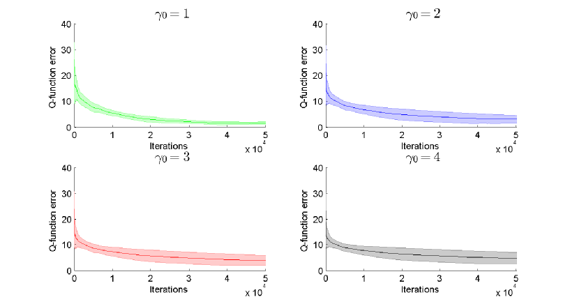
Figure 1: Evolution of the Q-function error, $\sum_{a\in{\cal A}}{{\|Q_{a}^{*}-{\hat{Q}}_{a,T}\|}_{\infty}}$ for the SPD Q-learning.

The evolutions of the dual policy error, $\sum_{s\in{\cal S}}{\|\pi_{s}^{*}-\hat{\pi}_{s,T}^{d}\|_{2}}$, obtained using Algorithm 1 for different $\gamma_{0}\in\{1,2,\ldots,4\}$, are given in Figure 2 (left-hand side).

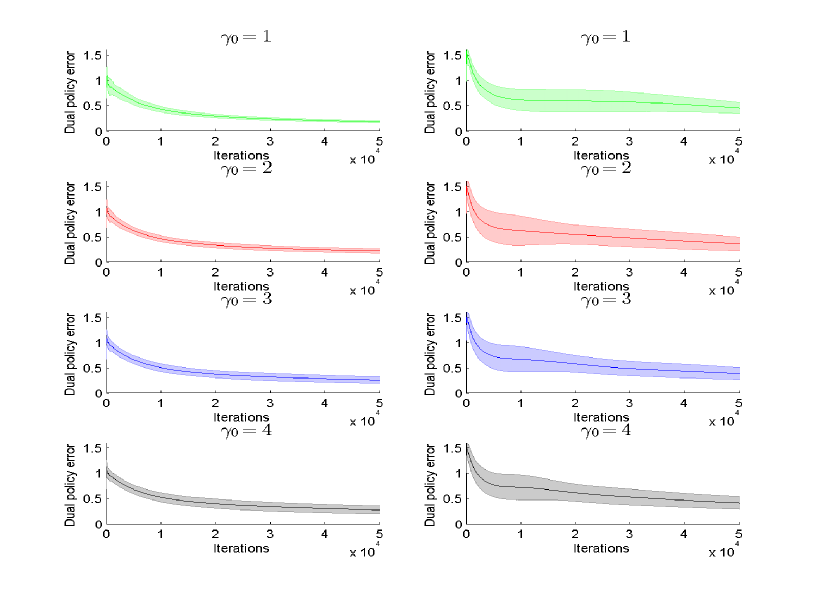
Figure 2: Evolution of the dual policy error, $\sum_{s\in{\cal S}}{\|\pi_{s}^{*}-\hat{\pi}_{s,T}^{d}\|_{\infty}}$, from the SPD Q-learning and the dual policy error, $\sum_{s\in{\cal S}}{\|\pi_{s}^{*}-\tilde{\pi}_{s,T}\|_{\infty}}$, from the SPD-RL in Chen and Wang (2016, Algorithm 1) with the importance sampling.

In the figure, the result is compared with the error, $\sum_{s\in{\cal S}}{\|\pi_{s}^{*}-\bar{\pi}_{s,T}\|_{\infty}}$ (right-hand side), of the stochastic policy $\bar{\pi}_{s,T}$ obtained by using the dual solutions of a modified Chen and Wang (2016, Algorithm 1) with $\eta=\sigma{\bf 1}_{|{\cal S}|}/|{\cal S}|$. Note that in the modified algorithm, the dual solutions of Chen and Wang (2016, Algorithm 1) are multiplied by $\hat{M}_{T}$, which estimates the true $M_{T}$ by sample averages so as to find the true optimal dual variables, and all algorithms for the comparison employ the step-size rule, $\gamma_{k}=\gamma_{0}/\sqrt{k+1},k\geq 0$. Figure 2 implies that both Algorithm 1 and modified Chen and Wang (2016, Algorithm 1) demonstrate similar convergence results in terms of the dual policy errors. Moreover, it shows that the dual policy from Algorithm 1 outperforms that from the modified SPD algorithm, Chen and Wang (2016, Algorithm 1). This is reasonable as the latter suffers from additional estimation errors.

Figure 3 shows the primal policy error (right-hand side), $\sum_{s\in{\cal S}}{\|\pi_{s}^{*}-\tilde{\pi}_{s,T}^{p}\|_{\infty}}$, where

$$\tilde{\pi}_{s,T}^{p}(s):=\begin{cases}\begin{bmatrix}1&0\\ \end{bmatrix}^{T}\quad{\rm if}\quad{\rm argmax}_{a\in{\cal A}}\hat{Q}_{a,T}(s)=1\\ \begin{bmatrix}0&1\\ \end{bmatrix}^{T}\quad{\rm if}\quad{\rm argmax}_{a\in{\cal A}}\hat{Q}_{a,T}(s)=2\\ \end{cases},$$

and the right-hand side figures are the policy error corresponding to the standard Q-learning. As one can see that, SPD Q-learning algorithm performs worse than the standard Q-learning on this simple task, which is more or less expected since Q-learning is a very powerful algorithm in practice. What’s interesting here is that, when comparing the dual policy error in Figure 2 to the primal policy error in Figure 3, it is clear that the primal policy of SPD Q-learning converges much faster than the dual policy. This demonstrates another potential advantage of the proposed algorithm over the existing primal-dual algorithm.

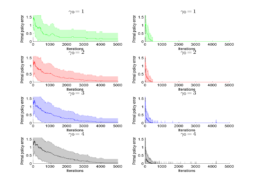
Figure 3: Evolution of the primal policy error, $\sum_{s\in{\cal S}}{\|\pi_{s}^{*}-\tilde{\pi}_{s,T}^{p}\|_{\infty}}$ (left-hand side), from the SPD Q-learning and the error of the standard Q-learning (right-hand side).

6.2 $2\times 2$ grid world

In this example, we consider a $2\times 2$ grid world, which simulates a path-planning problem for a mobile robot in an environment. The goal of the RL agent is to navigate from the starting point (left-bottom corner) to the goal (right-top corner), using four actions ${\cal A}=\{{\rm up,down,left,right}\}$. The behavior policy is defined as a stochastic policy which uniformly chooses one among the four actions. If the action leads the agent to escape the square boundary, then the location of the agent does not change. The reward is uniformly distributed in $[0,0.2]$ except for the reward at the goal state which is uniformly distributed in $[1,1.2]$. We run Algorithm 1 with $T=5000$, $\gamma_{k}=2/\sqrt{k+10000},k\geq 0$, $\eta=\frac{\sigma}{|{\cal S}|}\bf{1}_{|{\cal S}|}$, and $\alpha=0.9$.

Figure 4 illustrates the evolutions of the average reward corresponding to the primal policy of the SPD Q-learning (blue line) and the average reward of the standard Q-learning (green line). At each iteration step, the average rewards are obtained by the sample average of the rewards under the primal policy at the iteration step over eight time steps. The results show that the average reward of the SPD Q-learning converges to that of the standard Q-learning.

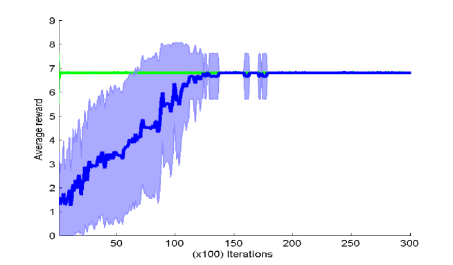
Figure 4: Evolution of the average reward corresponding to the primal policy of the SPD Q-learn ing (blue line) and the average reward of the standard Q-learning (green line).

7 Conclusion

In this paper, we introduce a new SPD-RL algorithm, where real-world observations under arbitrary behavior policies are used for finding a near-optimal policy. We prove the convergence with its sample complexity analysis. Promising future research directions are summarized as follows:

1. Safe RL: There exist scenarios where the safety of the RL agent is critical, where one should take into account the safety during and after the learning while maximizing the long-term reward. In this case, the dual LP (12) is useful in that the optimal dual variables represent the state-action distribution under the optimal policy. By imposing constraints on the dual variable in (12), we can shape the distribution by including prior knowledge of the task to design safer policies which avoid certain risks.

2. Distributed RL: In distributed RL (Lee et al., 2018), each agent receives local reward through a local processing, while communicating over sparse and random networks to learn the global value function corresponding to the aggregate of local rewards. The distributed learning can be formulated as a distributed optimization, and the frameworks in this paper can be applied for policy design problems.

3. Function approximation: The proposed SPD Q-learning framework can be easily combined with (linear or nonlinear) function approximations to handle large-scale or continuous state-action spaces. In this approach, both primal and dual variables need to be approximated by parameterized function classes, where important questions arise: if the algorithm converges, then how the resulting value function and policies can be interpreted? Can we derive meaningful optimality error bounds? It remains interesting to explore the theoretical and empirical convergence behaviors of the algorithm under such extensions.

Appendix A. Proof of Lemma 8

In this appendix, we prove Lemma 8 from Section 5:

Lemma Assume that there exists a real number $\zeta>0$ such that it is less than or equal to any diagonal element of $M$. Then, we have

$$\|\nabla_{x}L_{M_{k}}(x_{k},y_{k})+\varepsilon_{k}\|_{2}\leq\frac{\sqrt{13}|{\cal S}||{\cal A}|\|\eta\|_{1}}{\zeta(1-\alpha)}=:K_{1},$$

$$\|\nabla_{y}L_{M_{k}}(x_{k},y_{k})+\xi_{k}\|_{2}\leq\frac{\sqrt{13}|{\cal S}||{\cal A}|\sigma}{1-\alpha}=:K_{2}.$$

Proof  The first inequality follows by the chains of inequalities

$$\|\nabla_{x}L_{M_{k}}(x_{k},y_{k})+\varepsilon_{k}\|_{2}$$

$$=\left\|\begin{bmatrix}(e_{\hat{s}_{k}}\otimes e_{\hat{a}_{k}})e_{\hat{s}_{k}}^{T}|{\cal S}||{\cal A}|\lambda_{\hat{a}_{k}}^{(k)}-(e_{s_{k}}\otimes e_{a_{k}})e_{s_{k}}^{T}\mu_{a_{k}}^{(k)}\\ e_{\hat{s}_{k}}e_{\hat{s}_{k}}^{T}|{\cal S}|\eta-e_{\hat{s}_{k}}e_{\hat{s}_{k}}^{T}|{\cal S}||{\cal A}|\lambda_{\hat{a}_{k}}^{(k)}+\alpha e_{s_{k+1}}e_{s_{k}}^{T}\mu_{a_{k}}^{(k)}\\ \end{bmatrix}\right\|_{2}$$

$$=(\|(e_{\hat{s}_{k}}\otimes e_{\hat{a}_{k}})e_{\hat{s}_{k}}^{T}|{\cal S}||{\cal A}|\lambda_{\hat{a}_{k}}^{(k)}-(e_{s_{k}}\otimes e_{a_{k}})e_{s_{k}}^{T}\mu_{a_{k}}^{(k)}\|_{2}^{2}$$

$$+\|e_{\hat{s}_{k}}e_{\hat{s}_{k}}^{T}|{\cal S}|\eta-e_{\hat{s}_{k}}e_{\hat{s}_{k}}^{T}|{\cal S}||{\cal A}|\lambda_{\hat{a}_{k}}^{(k)}+\alpha e_{s_{k+1}}e_{s_{k}}^{T}\mu_{a_{k}}^{(k)}\|_{2}^{2})^{1/2}$$

$$\leq(2|{\cal S}|^{2}|{\cal A}|^{2}\|\lambda^{(k)}\|_{\infty}^{2}+2\|\mu^{(k)}\|_{\infty}^{2}+3|{\cal S}|^{2}\|\eta\|_{\infty}^{2}+3|{\cal S}|^{2}|{\cal A}|^{2}\|\lambda^{(k)}\|_{\infty}^{2}+\alpha^{2}3\|\mu^{(k)}\|_{\infty}^{2})^{1/2}$$

$$\leq\left(\frac{5|{\cal S}|^{2}|{\cal A}|^{2}\|\eta\|_{1}^{2}}{(1-\alpha)^{2}}+\frac{5\|\eta\|_{1}^{2}}{\zeta^{2}(1-\alpha)^{2}}+3|{\cal S}|^{2}\|\eta\|_{\infty}^{2}\right)^{1/2}$$

$$\leq\frac{\sqrt{13}|{\cal S}||{\cal A}|\|\eta\|_{1}}{\zeta(1-\alpha)},$$ (43)

where the first inequality follows from the vector inequality $\|v_{1}+v_{2}+\cdots+v_{n}\|_{2}^{2}\leq n(\|v_{1}\|_{2}^{2}+\|v_{2}\|_{2}^{2}+\cdots+\|v_{n}\|_{2}^{2})$ for any vectors $v_{1},\ldots,v_{n}$ and $\|e_{\hat{s}_{k}}e_{\hat{s}_{k}}^{T}\lambda_{\hat{a}_{k}}^{(k)}\|_{2}^{2}\leq\|\lambda^{(k)}\|_{\infty}^{2},\|e_{s_{k+1}}e_{s_{k}}^{T}\mu_{a_{k}}^{(k)}\|_{2}^{2}\leq\|\mu^{(k)}\|_{\infty}^{2}$, the second inequality follows from Lemma 6 and the last inequality is obtained after simplifications. For the second result, we have

$$\|\nabla_{y}L_{M_{k}}(x_{k},y_{k})+\xi_{k}\|_{2}$$

$$=\left\|\begin{bmatrix}|{\cal S}||{\cal A}|[(e_{\hat{s}_{k}}\otimes e_{\hat{a}_{k}})e_{\hat{s}_{k}}^{T}Q_{\hat{a}_{k}}^{(k)}-(e_{\hat{s}_{k}}\otimes e_{\hat{a}_{k}})e_{\hat{s}_{k}}^{T}V^{(k)}]\\ \alpha e_{s_{k}}e_{s_{k+1}}^{T}V^{(k)}+e_{s_{k}}\hat{r}(s_{k},a_{k},s_{k+1})-e_{s_{k}}e_{s_{k}}^{T}Q_{a_{k}}^{(k)}\\ \end{bmatrix}\right\|_{2}$$

$$=(\||{\cal S}||{\cal A}|[(e_{\hat{s}_{k}}\otimes e_{\hat{a}_{k}})e_{\hat{s}_{k}}^{T}Q_{\hat{a}_{k}}^{(k)}-(e_{\hat{s}_{k}}\otimes e_{\hat{a}_{k}})e_{\hat{s}_{k}}^{T}V^{(k)}]\|_{2}^{2}$$

$$+\|\alpha e_{s_{k}}e_{s_{k+1}}^{T}V^{(k)}+e_{s_{k}}\hat{r}(s_{k},a_{k},s_{k+1})-e_{s_{k}}e_{s_{k}}^{T}Q_{a_{k}}^{(k)}\|_{2}^{2})^{1/2}$$

$$\leq(2|{\cal S}|^{2}|{\cal A}|^{2}\|Q^{(k)}\|_{\infty}^{2}+2\|V^{(k)}\|_{\infty}^{2}+3\alpha^{2}\|V^{(k)}\|_{\infty}^{2}+3\sigma^{2}+3\|Q^{(k)}\|_{\infty}^{2})^{1/2}$$

$$\leq\left(2|{\cal S}|^{2}|{\cal A}|^{2}\frac{\sigma^{2}}{(1-\alpha)^{2}}+2|{\cal S}|^{2}|{\cal A}|^{2}\frac{\sigma^{2}}{(1-\alpha)^{2}}+3\alpha^{2}\frac{\sigma^{2}}{(1-\alpha)^{2}}+3\sigma^{2}+3\frac{\sigma^{2}}{(1-\alpha)^{2}}\right)^{1/2}$$

$$\leq\sqrt{13}\frac{|{\cal S}||{\cal A}|\sigma}{1-\alpha},$$

where the first inequality follows from the vector inequality $\left\|{v_{1}+v_{2}+\cdots+v_{n}}\right\|_{2}^{2}\leq n(\left\|{v_{1}}\right\|_{2}^{2}+\left\|{v_{2}}\right\|_{2}^{2}+\cdots+\left\|{v_{n}}\right\|_{2}^{2})$ for any vectors $v_{1},\ldots,v_{n}$ and $\|e_{s_{k}}e_{s_{k+1}}^{T}V^{(k)}\|_{2}^{2}\leq\|V^{(k)}\|_{\infty}^{2},\|e_{s_{k}}e_{s_{k}}^{T}Q_{a_{k}}^{(k)}\|_{2}^{2}\leq\|Q^{(k)}\|_{\infty}^{2}$, the second inequality follows from Lemma 6, and the last inequality follows after simplifications.  

Appendix B. Proof of Lemma 9

In this appendix, we prove Lemma 9 from Section 5:

Lemma Assume that there exists a real number $\zeta>0$ such that it is less than or equal to any diagonal element of $M$. Then, we have

$$\Phi_{1}(x^{*})\leq\frac{2\sigma^{2}|{\cal S}|}{(1-\alpha)^{2}}\frac{1}{\gamma_{T-1}},$$

$$\Phi_{2}(y^{*})\leq\frac{1}{\gamma_{T-1}}\frac{4\|\eta\|_{1}^{2}}{\zeta^{4}(1-\alpha)^{2}}+\frac{2\|\eta\|_{1}^{2}}{\zeta^{3}(1-\alpha)^{2}}\sum_{k=1}^{T-1}{\frac{\beta_{k-1}}{\gamma_{k-1}}}.$$

Proof  First, $\Phi_{1}(x^{*})$ is bounded by using the chains of inequalities

$$\Phi_{1}(x^{*}) =\sum_{k=0}^{T-1}{\frac{1}{2\gamma_{k}}({\cal E}_{k}^{(1)}(x^{*})-{\cal E}_{k+1}^{(1)}(x^{*}))}$$

$$\leq\frac{1}{2}\left(\frac{1}{\gamma_{0}}{\cal E}_{0}^{(1)}(x^{*})+\sum_{k=0}^{T-2}{\left(\frac{1}{\gamma_{k+1}}-\frac{1}{\gamma_{k}}\right){\cal E}_{k+1}^{(1)}(x^{*})}\right)$$

$$=\frac{1}{2}\left(\frac{1}{\gamma_{0}}\|x_{0}-x^{*}\|_{2}^{2}+\sum_{k=0}^{T-2}{\left(\frac{1}{\gamma_{k+1}}-\frac{1}{\gamma_{k}}\right)\|x_{k+1}-x^{*}\|_{2}^{2}}\right)$$

$$\leq\frac{1}{2}\frac{1}{\gamma_{0}}(\|x_{0}\|_{2}^{2}+\|x^{*}\|_{2}^{2}+2\|x_{0}\|_{2}\|x^{*}\|_{2})$$

$$+\frac{1}{2}\sum_{k=0}^{T-2}{\left(\frac{1}{\gamma_{k+1}}-\frac{1}{\gamma_{k}}\right)(\|x_{k+1}\|_{2}^{2}+\|x^{*}\|_{2}^{2}+2\|x_{k+1}\|_{2}\|x^{*}\|_{2})}$$ (44)

$$\leq\frac{1}{2}\frac{4\sigma^{2}|{\cal S}|}{(1-\alpha)^{2}}\left(\frac{1}{\gamma_{0}}+\sum_{k=0}^{T-2}{\left(\frac{1}{\gamma_{k+1}}-\frac{1}{\gamma_{k}}\right)}\right)$$ (45)

$$=\frac{2\sigma^{2}|{\cal S}|}{(1-\alpha)^{2}}\frac{1}{\gamma_{T-1}},$$

where (44) follows from the relation $\|a-b\|_{2}^{2}=\|a\|_{2}^{2}+\|b\|_{2}^{2}-2a^{T}b$ and Cauchy-Schwarz inequality and (45) is due to $x_{k},x^{*}\in{\cal X}$. Similarly, we have

$$\Phi_{2}(y^{*}) =\frac{1}{2}\sum_{k=0}^{T-1}{\frac{1}{\gamma_{k}}({\cal E}_{k}^{(2)}(\bar{M}_{k}^{-1}y^{*})-{\cal E}_{k+1}^{(2)}(\bar{M}_{k}^{-1}y^{*}))}$$

$$\leq\frac{1}{2}\left(\frac{1}{\gamma_{0}}{\cal E}_{0}^{(2)}(\bar{M}_{0}^{-1}y^{*})+\sum_{k=1}^{T-1}{\left(\frac{1}{\gamma_{k}}{\cal E}_{k}^{(2)}(\bar{M}_{k}^{-1}y^{*})-\frac{1}{\gamma_{k-1}}{\cal E}_{k}^{(2)}(\bar{M}_{k-1}^{-1}y^{*})\right)}\right)$$

$$=\frac{1}{2}\frac{1}{\gamma_{0}}{\cal E}_{0}^{(2)}(\bar{M}_{0}^{-1}y^{*})+\frac{1}{2}\sum_{k=1}^{T-1}{\left(\frac{1}{\gamma_{k}}-\frac{1}{\gamma_{k-1}}\right){\cal E}_{k}^{(2)}(\bar{M}_{k}^{-1}y^{*})}$$

$$+\frac{1}{2}\sum_{k=1}^{T-1}{\frac{1}{\gamma_{k-1}}({\cal E}_{k}^{(2)}(\bar{M}_{k}^{-1}y^{*})-{\cal E}_{k}^{(2)}(\bar{M}_{k-1}^{-1}y^{*}))},$$ (46)

where the last equality is obtained by rearranging terms. For any $k\geq 0$, ${\cal E}_{k}^{(2)}(\bar{M}_{k}^{-1}y^{*})$ is bounded as

$${\cal E}_{k}^{(2)}(\bar{M}_{k}^{-1}y^{*}) =\|y_{k}-\bar{M}_{k}^{-1}y^{*}\|_{2}^{2}$$

$$=\|y_{k}\|_{2}^{2}+\|\bar{M}_{k}^{-1}y^{*}\|_{2}^{2}-2y_{k}^{T}\bar{M}_{k}^{-1}y^{*}$$

$$\leq\|y_{k}\|_{2}^{2}+\|\bar{M}_{k}^{-1}y^{*}\|_{2}^{2}+2\|y_{k}\|_{2}\|\bar{M}_{k}^{-1}y^{*}\|_{2}$$

$$\leq\|y_{k}\|_{2}^{2}+\|\bar{M}_{k}^{-1}\|_{2}^{2}\|y^{*}\|_{2}^{2}+2\|y_{k}\|_{2}\|\bar{M}_{k}^{-1}\|_{2}\|y^{*}\|_{2}$$

$$\leq\|y_{k}\|_{2}^{2}+\zeta^{-2}\|y^{*}\|_{2}^{2}+2\|y_{k}\|_{2}\zeta^{-1}\|y^{*}\|_{2}$$

$$\leq\frac{\|\eta\|_{1}^{2}}{\zeta^{2}(1-\alpha)^{2}}+\zeta^{-2}\frac{\|\eta\|_{1}^{2}}{\zeta^{2}(1-\alpha)^{2}}+2\zeta^{-1}\frac{\|\eta\|_{1}^{2}}{\zeta^{2}(1-\alpha)^{2}}$$

$$\leq\frac{4\|\eta\|_{1}^{2}}{\zeta^{4}(1-\alpha)^{2}},$$

where the first inequality is due to the Cauchy-Schwarz inequality, the fourth inequality is due to Lemma 6, and the last inequality follows using $\zeta<1$. Upon substituting the above inequality into (46), we obtain

$$\Phi_{2}(y^{*})\leq\frac{1}{\gamma_{T-1}}\frac{4\|\eta\|_{1}^{2}}{\zeta^{4}(1-\alpha)^{2}}+\frac{1}{2}\sum_{k=1}^{T-1}{\frac{1}{\gamma_{k-1}}({\cal E}_{k}^{(2)}(\bar{M}_{k}^{-1}y^{*})-{\cal E}_{k}^{(2)}(\bar{M}_{k-1}^{-1}y^{*}))}.$$ (47)

The second term in (47) is written as

$$\frac{1}{2}\sum_{k=1}^{T-1}{\frac{1}{\gamma_{k-1}}({\cal E}_{k}^{(2)}(\bar{M}_{k}^{-1}y^{*})-{\cal E}_{k}^{(2)}(\bar{M}_{k-1}^{-1}y^{*}))}$$

$$=\frac{1}{2}\sum_{k=1}^{T-1}{\frac{1}{\gamma_{k-1}}(\|y_{k}-\bar{M}_{k}^{-1}y^{*}\|_{2}^{2}-\|y_{k}-\bar{M}_{k-1}^{-1}y^{*}\|_{2}^{2})}$$

$$=\frac{1}{2}\sum_{k=1}^{T-1}{\frac{1}{\gamma_{k-1}}(\|\bar{M}_{k}^{-1}y^{*}\|_{2}^{2}+\|y_{k}\|_{2}^{2}-2y_{k}^{T}\bar{M}_{k}^{-1}y^{*}-\|\bar{M}_{k-1}^{-1}y^{*}\|_{2}^{2}-\|y_{k}\|_{2}^{2}+2y_{k}^{T}\bar{M}_{k-1}^{-1}y^{*})}$$ (48)

$$=\frac{1}{2}\sum_{k=1}^{T-1}{\frac{1}{\gamma_{k-1}}((y^{*})^{T}(\bar{M}_{k}^{-1}\bar{M}_{k}^{-1}-\bar{M}_{k-1}^{-1}\bar{M}_{k-1}^{-1})y^{*}+2y_{k}^{T}(\bar{M}_{k-1}^{-1}-\bar{M}_{k}^{-1})y^{*})}$$

$$=\frac{1}{2}\sum_{k=1}^{T-1}{\frac{1}{\gamma_{k-1}}(y^{*}(\bar{M}_{k}^{-1}-\bar{M}_{k-1}^{-1})(\bar{M}_{k}^{-1}+\bar{M}_{k-1}^{-1})y^{*}+2y_{k}^{T}(\bar{M}_{k-1}^{-1}-\bar{M}_{k}^{-1})y^{*})}$$ (49)

$$\leq\frac{1}{2}\sum_{k=1}^{T-1}{\frac{1}{\gamma_{k-1}}(\|y^{*}\|_{2}^{2}\|\bar{M}_{k-1}^{-1}-\bar{M}_{k}^{-1}\|_{2}\|\bar{M}_{k-1}^{-1}+\bar{M}_{k}^{-1}\|_{2}+2\|y_{k}\|_{2}\|y^{*}\|_{2}\|\bar{M}_{k-1}^{-1}-\bar{M}_{k}^{-1}\|_{2})}$$

$$\leq\frac{1}{2}\frac{\|\eta\|_{1}^{2}}{\zeta^{2}(1-\alpha)^{2}}\sum_{k=1}^{T-1}{\frac{1}{\gamma_{k-1}}(\|\bar{M}_{k-1}^{-1}-\bar{M}_{k}^{-1}\|_{2}\|\bar{M}_{k-1}^{-1}+\bar{M}_{k}^{-1}\|_{2}+2\|\bar{M}_{k-1}^{-1}-\bar{M}_{k}^{-1}\|_{2})}$$ (50)

$$\leq\frac{1}{2}\frac{\|\eta\|_{1}^{2}}{\zeta^{2}(1-\alpha)^{2}}\sum_{k=1}^{T-1}{\frac{1}{\gamma_{k-1}}(\|\bar{M}_{k-1}^{-1}-\bar{M}_{k}^{-1}\|_{2}\frac{2}{\zeta}+2\|\bar{M}_{k-1}^{-1}-\bar{M}_{k}^{-1}\|_{2})}$$ (51)

$$=\frac{\|\eta\|_{1}^{2}}{\zeta^{2}(1-\alpha)^{2}}\left(1+\frac{1}{\zeta}\right)\sum_{k=1}^{T-1}{\frac{\|\bar{M}_{k-1}^{-1}-\bar{M}_{k}^{-1}\|}{\gamma_{k-1}}}$$

$$\leq\frac{2\|\eta\|_{1}^{2}}{\zeta^{3}(1-\alpha)^{2}}\sum_{k=1}^{T-1}{\frac{\beta_{k-1}}{\gamma_{k-1}}},$$

where (48) follows from the relation $\|a-b\|_{2}^{2}=\|a\|_{2}^{2}+\|b\|_{2}^{2}-2a^{T}b$ for any vectors $a,b$, (49) follows from $(\bar{M}_{k}^{-1}-\bar{M}_{k-1}^{-1})(\bar{M}_{k}^{-1}+\bar{M}_{k-1}^{-1})=\bar{M}_{k}^{-1}\bar{M}_{k}^{-1}-\bar{M}_{k-1}^{-1}\bar{M}_{k-1}^{-1}$, (50) is due to $y_{k},y_{T}^{*}\in{\cal Y}$, (51) follows from the triangle inequality and $\|\bar{M}_{k}^{-1}\|_{2}\leq\zeta^{-1}$, and the last inequality comes from 3. Combining the last inequality with (47) yields the second conclusion. This completes the proof.  

Appendix C. Proof of Lemma 11

In this appendix, we prove Lemma 11 from Section 5:

Lemma We have $\Delta{\cal G}_{T+1}={\cal G}_{T+1}-{\cal G}_{T}=\frac{1}{2\gamma_{T}}({\cal E}_{T+1}-{\mathbb{E}}[{\cal E}_{T+1}|{\cal F}_{T}])\leq b$ with probability one, where

$$b=\frac{13\gamma_{0}\|\eta\|_{1}+13\gamma_{0}\zeta^{2}\sigma^{2}+16\sqrt{26}\sigma\zeta\|\eta\|_{1}}{2}\frac{|{\cal S}|^{2}|{\cal A}|^{2}}{\zeta^{2}(1-\alpha)^{2}}.$$

Proof  Note that

$${\cal G}_{T+1}-{\cal G}_{T}=\frac{1}{2\gamma_{T}}({\cal E}_{T+1}^{(1)}(x_{T}^{*})-{\mathbb{E}}[{\cal E}_{T+1}^{(1)}(x_{T}^{*})|{\cal F}_{T}])+\frac{1}{2\gamma_{T}}({\cal E}_{T+1}^{(2)}(\bar{M}_{T+1}^{-1}y_{T}^{*})-{\mathbb{E}}[{\cal E}_{T+1}^{(2)}(\bar{M}_{T+1}^{-1}y_{T}^{*})|{\cal F}_{T}]),$$

and we first derive a bound on $\frac{1}{2\gamma_{T}}({\cal E}_{T+1}^{(1)}(x_{T}^{*})-{\mathbb{E}}[{\cal E}_{T+1}^{(1)}(x_{T}^{*})|{\cal F}_{T}])$. Using the definition of ${\cal E}_{k+1}^{(1)}(x_{T}^{*})$ yields

$$\frac{1}{2\gamma_{T}}({\cal E}_{T+1}^{(1)}(x_{T}^{*})-{\mathbb{E}}[{\cal E}_{T+1}^{(1)}(x_{T}^{*})|{\cal F}_{T}])=\frac{1}{2\gamma_{T}}\|\Pi_{\cal X}(x_{T}-\gamma_{T}\nabla_{x}L_{G_{k}}(x_{T},y_{T})-\gamma_{T}\varepsilon_{T})-x_{T}^{*}\|_{2}^{2}$$

$$-\frac{1}{2\gamma_{T}}{\mathbb{E}}[\|\Pi_{\cal X}(x_{T}-\gamma_{T}\nabla_{x}L_{G_{T}}(x_{T},y_{T})-\gamma_{T}\varepsilon_{T})-x_{T}^{*}\|_{2}^{2}|{\cal F}_{T}].$$ (52)

Noting

$$\|\Pi_{\cal X}(x_{T}-\gamma_{T}\nabla_{x}L_{G_{T}}(x_{T},y_{T})-\gamma_{T}\varepsilon_{T})-x_{T}^{*}\|_{2}^{2}$$

$$=\|\Pi_{\cal X}(x_{T}-\gamma_{T}\nabla_{x}L_{T}(x_{T},y_{T})-\gamma_{T}\varepsilon_{T})-x_{T}\|_{2}^{2}+\|x_{T}-x_{T}^{*}\|_{2}^{2}$$

$$-2(x_{T}-x_{T}^{*})^{T}(\Pi_{\cal X}(x_{T}-\gamma_{T}\nabla_{x}L_{T}(x_{T},y_{T})-\gamma_{T}\varepsilon_{T})-x_{T})$$

it follows from (52) that

$$\frac{1}{2\gamma_{T}}({\cal E}_{T+1}^{(1)}(x_{T}^{*})-{\mathbb{E}}[{\cal E}_{T+1}^{(1)}(x_{T}^{*})|{\cal F}_{T}])$$

$$=\frac{1}{2\gamma_{T}}\|\Pi_{\cal X}(x_{T}-\gamma_{T}\nabla_{x}L_{G_{T}}(x_{T},y_{T})-\gamma_{T}\varepsilon_{T})-x_{T}\|_{2}^{2}+\frac{1}{2\gamma_{T}}\|x_{T}-x_{T}^{*}\|_{2}^{2}$$

$$-\frac{1}{\gamma_{T}}(x_{T}-x_{T}^{*})^{T}(\Pi_{\cal X}(x_{T}-\gamma_{T}\nabla_{x}L_{G_{T}}(x_{T},y_{T})-\gamma_{T}\varepsilon_{T})-x_{T})$$

$$-\frac{1}{2\gamma_{T}}{\mathbb{E}}[\|\Pi_{\cal X}(x_{T}-\gamma_{T}\nabla_{x}L_{G_{T}}(x_{T},y_{T})-\gamma_{T}\varepsilon_{T})-x_{T}\|_{2}^{2}|{\cal F}_{T}]-\frac{1}{2\gamma_{T}}\|x_{T}-x_{T}^{*}\|_{2}^{2}$$

$$+\frac{1}{\gamma_{T}}{\mathbb{E}}[(\Pi_{\cal X}(x_{T}-\gamma_{T}\nabla_{x}L_{G_{T}}(x_{T},y_{T})-\gamma_{T}\varepsilon_{T})-x_{T})^{T}(x_{T}-x_{T}^{*})|{\cal F}_{T}]$$

$$\leq\frac{1}{2\gamma_{T}}\|\Pi_{\cal X}(x_{T}-\gamma_{T}\nabla_{x}L_{T}(x_{T},y_{T})-\gamma_{T}\varepsilon_{T})-x_{T}\|_{2}^{2}$$

$$+\frac{1}{\gamma_{T}}\|x_{T}-x_{T}^{*}\|_{2}\|\Pi_{\cal X}(x_{T}-\gamma_{T}\nabla_{x}L_{T}(x_{T},y_{T})-\gamma_{T}\varepsilon_{T})-x_{T}\|_{2}$$

$$+\frac{1}{\gamma_{T}}{\mathbb{E}}[\|x_{T}-x_{T}^{*}\|_{2}\|\Pi_{\cal X}(x_{T}-\gamma_{T}\nabla_{x}L_{T}(x_{T},y_{T})-\gamma_{T}\varepsilon_{k})-x_{T}\|_{2}|{\cal F}_{T}]$$ (53)

$$\leq\frac{\gamma_{T}}{2}\|\nabla_{x}L_{T}(x_{T},y_{T})+\varepsilon_{T}\|_{2}^{2}+\|x_{T}-x_{T}^{*}\|_{2}\|\nabla_{x}L_{T}(x_{T},y_{T})+\varepsilon_{T}\|_{2}$$

$$+\|x_{T}-x_{T}^{*}\|_{2}{\mathbb{E}}[\|\nabla_{x}L_{T}(x_{T},y_{T})+\varepsilon_{T}\|_{2}|{\cal F}_{T}]$$ (54)

$$\leq\frac{1}{2}(\gamma_{T}K_{1}^{2}+4K_{1}\|x_{T}-x_{T}^{*}\|_{2})$$

$$\leq\frac{1}{2}\left(\gamma_{0}\left(\frac{\sqrt{13}|{\cal S}||{\cal A}|\|\eta\|_{1}}{\zeta(1-\alpha)}\right)^{2}+4\left(\frac{\sqrt{13}|{\cal S}||{\cal A}|\|\eta\|_{1}}{\zeta(1-\alpha)}\right)\sqrt{|{\cal S}||{\cal A}|+|{\cal S}|}\|x_{T}-x_{T}^{*}\|_{\infty}\right)$$

$$\leq\frac{13\gamma_{0}+8\sqrt{26}\sigma\zeta}{2}\frac{|{\cal S}|^{2}|{\cal A}|^{2}\|\eta\|_{1}}{\zeta^{2}(1-\alpha)^{2}},$$

where (53) follows from the Cauchy-Schwarz inequality, (54) follows from the nonexpansive map property of the projection $\|\Pi_{\cal X}(a)-\Pi_{\cal X}(b)\|_{2}\leq\|a-b\|_{2}$, and the last inequality is obtained after simplifications. Using similar lines, one obtains

$$\frac{1}{2\gamma_{T}}({\cal E}_{T+1}^{(2)}(\bar{M}_{T}^{-1}y_{T}^{*})-{\mathbb{E}}[{\cal E}_{T+1}^{(2)}(\bar{M}_{T}^{-1}y_{T}^{*})|{\cal F}_{T}])\leq\frac{13\gamma_{0}\zeta^{2}\sigma+8\sqrt{26}\zeta\|\eta\|_{1}}{2}\frac{\sigma|{\cal S}|^{2}|{\cal A}|^{2}}{\zeta^{2}(1-\alpha)^{2}},$$

and combining the two inequalities completes the proof.  

Appendix D. Proof of Lemma 12

In this appendix, we prove Lemma 12 from Section 5:

Lemma $\frac{1}{T}\langle{\cal G}\rangle_{T}\leq a$ holds with probability one, where

$$a=\frac{1}{4}\frac{(\gamma_{0}(13\|\eta\|_{1}+4\sqrt{26}\sigma\zeta)\|\eta\|_{1}+13\gamma_{0}\zeta^{2}\sigma^{2}+4\sqrt{26}\sigma\|\eta\|_{1})^{2}|{\cal S}|^{4}|{\cal A}|^{4}}{\zeta^{4}(1-\alpha)^{4}}.$$

Proof  Using ${\mathbb{E}}[{\cal E}_{k}|{\cal F}_{k}]={\cal E}_{k}$, we have

$${\mathbb{E}}[|{\cal G}_{k+1}-{\cal G}_{k}|^{2}|{\cal F}_{k}] =\frac{1}{4\gamma_{k}^{2}}{\mathbb{E}}[|{\cal E}_{k+1}-{\mathbb{E}}[{\cal E}_{k+1}|{\cal F}_{k}]|^{2}|{\cal F}_{k}]$$

$$=\frac{1}{4\gamma_{k}^{2}}{\mathbb{E}}[|{\cal E}_{k+1}-{\cal E}_{k}-{\mathbb{E}}[{\cal E}_{k+1}-{\cal E}_{k}|{\cal F}_{k}]|^{2}|{\cal F}_{k}]$$

$$\leq\frac{1}{4\gamma_{k}^{2}}{\mathbb{E}}[{\mathbb{E}}[|{\cal E}_{k+1}-{\cal E}_{k}|^{2}|{\cal F}_{k}]|{\cal F}_{k}]$$

$$=\frac{1}{4\gamma_{k}^{2}}{\mathbb{E}}[|\underbrace{{\cal E}_{k+1}^{(1)}(x_{T}^{*})+{\cal E}_{k+1}^{(2)}(\bar{M}_{k+1}^{-1}y_{T}^{*})-{\cal E}_{k}^{(1)}(x_{T}^{*})-{\cal E}_{k}^{(2)}(\bar{M}_{k+1}^{-1}y_{T}^{*})}_{=:\Upsilon_{1}}|^{2}|{\cal F}_{k}],$$ (55)

where the inequality follows from the fact that the variance of a random variable is bounded by its second moment. For bounding (55), note that $\Phi_{1}$ is written as

$$\Upsilon_{1}=\|x_{k+1}-x_{T}^{*}\|_{2}^{2}-\|x_{k}-x_{T}^{*}\|_{2}^{2}+\|y_{k+1}-\bar{M}_{k+1}^{-1}y_{T}^{*}\|_{2}^{2}-\|y_{k}-\bar{M}_{k+1}^{-1}y_{T}^{*}\|_{2}^{2}$$

and $|\Upsilon_{1}|\leq|\|x_{k+1}-x_{T}^{*}\|^{2}-\|x_{k}-x_{T}^{*}\|^{2}|+|\|y_{k+1}-\bar{M}_{k+1}^{-1}y_{T}^{*}\|^{2}-\|y_{k}-\bar{M}_{k+1}^{-1}y_{T}^{*}\|^{2}|$.

Here, the first two terms have the bound

$$|\|x_{k+1}-x_{T}^{*}\|^{2}-\|x_{k}-x_{T}^{*}\|^{2}|$$

$$=|\|\Pi_{\cal X}(x_{k}-\gamma_{k}\nabla_{x}L_{k}(x_{k},y_{k})-\gamma_{k}\varepsilon_{k})-x_{k}\|^{2}$$

$$-2(\Pi_{\cal X}(x_{k}-\gamma_{k}\nabla_{x}L_{k}(x_{k},y_{k})-\gamma_{k}\varepsilon_{k})-x_{k})^{T}(x_{k}-x_{T}^{*})|$$ (56)

$$\leq\|\Pi_{\cal X}(x_{k}-\gamma_{k}\nabla_{x}L_{k}(x_{k},y_{k})-\gamma_{k}\varepsilon_{k})-x_{k}\|_{2}^{2}$$

$$+2\|\Pi_{\cal X}(x_{k}-\gamma_{k}\nabla_{x}L_{k}(x_{k},y_{k})-\gamma_{k}\varepsilon_{k})-x_{k}\|_{2}\|x_{k}-x_{T}^{*}\|_{2}$$ (57)

$$\leq\gamma_{k}^{2}\|\nabla_{x}L_{k}(x_{k},y_{k})+\varepsilon_{k}\|_{2}^{2}+2\gamma_{k}\|\nabla_{x}L_{k}(x_{k},y_{k})+\varepsilon_{k}\|_{2}\|x_{k}-x_{T}^{*}\|_{2}$$ (58)

$$\leq\gamma_{k}^{2}K_{1}^{2}+2\gamma_{k}K_{1}\sqrt{|{\cal S}||{\cal A}|+|{\cal S}|}\|x_{k}-x_{T}^{*}\|_{\infty}$$ (59)

$$\leq\gamma_{k}^{2}\left(\frac{\sqrt{13}|{\cal S}||{\cal A}|\|\eta\|_{1}}{\zeta(1-\alpha)}\right)^{2}+2\gamma_{k}\frac{\sqrt{13}|{\cal S}||{\cal A}|\|\eta\|_{1}}{\zeta(1-\alpha)}\sqrt{2|{\cal S}||{\cal A}|}\frac{2\sigma}{1-\alpha}$$

$$\leq\gamma_{k}\frac{\gamma_{0}(13\|\eta\|_{1}+4\sqrt{26}\sigma\zeta)|{\cal S}|^{2}|{\cal A}|^{2}\|\eta\|_{1}}{\zeta^{2}(1-\alpha)^{2}},$$

where (56) follows from the relation $\|a-b\|_{2}^{2}=\|a\|_{2}^{2}+\|b\|_{2}^{2}-2a^{T}b$ for any vectors $a,b$, (57) follows from the Cauchy-Schwarz inequality, (58) is due to the nonexpansive map property of the projection $\|\Pi_{\cal X}(a)-\Pi_{\cal X}(b)\|_{2}\leq\|a-b\|_{2}$, (59) comes from Lemma 8 and the inequality $\|a\|_{2}\leq\sqrt{n}\|a\|_{\infty}$ for any $a\in{\mathbb{R}}^{n}$, and the last inequality follows from algebraic simplifications. Similarly, the second two terms in $\Phi_{1}$ are bounded as

$$|\|y_{k+1}-\bar{M}_{k+1}^{-1}y_{T}^{*}\|^{2}-\|y_{k}-\bar{M}_{k+1}^{-1}y_{T}^{*}\|^{2}|$$

$$=|\|\Pi_{\cal Y}(y_{k}-\gamma_{k}\nabla_{y}L_{M_{k}}(x_{k},y_{k})-\gamma_{k}\xi_{k})-y_{k}\|^{2}$$

$$-2(\Pi_{\cal Y}(y_{k}-\gamma_{k}\nabla_{y}L_{M_{k}}(x_{k},y_{k})-\gamma_{k}\xi_{k})-y_{k})(y_{k}-\bar{M}_{k+1}^{-1}y_{T}^{*})|$$

$$\leq\|\Pi_{\cal Y}(y_{k}-\gamma_{k}\nabla_{y}L_{M_{k}}(x_{k},y_{k})-\gamma_{k}\xi_{k})-y_{k}\|_{2}^{2}$$

$$+2\|\Pi_{\cal Y}(y_{k}-\gamma_{k}\nabla_{y}L_{M_{k}}(x_{k},y_{k})-\gamma_{k}\xi_{k})-y_{k}\|_{2}\|y_{k}-\bar{M}_{k+1}^{-1}y_{T}^{*}\|_{2}$$

$$\leq\gamma_{k}^{2}\|\nabla_{y}L_{M_{k}}(x_{k},y_{k})+\xi_{k}\|_{2}^{2}+2\gamma_{k}\|\nabla_{y}L_{M_{k}}(x_{k},y_{k})+\xi_{k}\|_{2}\|y_{k}-\bar{M}_{k+1}^{-1}y_{T}^{*}\|_{2}$$

$$\leq\gamma_{k}^{2}K_{2}^{2}+2\gamma_{k}K_{2}\sqrt{2|{\cal S}||{\cal A}|}(\|y_{k}\|_{\infty}+\|\bar{M}_{k+1}^{-1}\|_{\infty}\|y_{T}^{*}\|_{\infty})$$

$$\leq\gamma_{k}\frac{(13\gamma_{0}\zeta^{2}\sigma^{2}+4\sqrt{26}\sigma\|\eta\|_{1})|{\cal S}|^{2}|{\cal A}|^{2}}{\zeta^{2}(1-\alpha)^{2}}.$$

Combining the last two results leads to

$$|\Upsilon_{1}|\leq\gamma_{k}\frac{(\gamma_{0}(13\|\eta\|_{1}+4\sqrt{26}\sigma\zeta)\|\eta\|_{1}+13\gamma_{0}\zeta^{2}\sigma^{2}+4\sqrt{26}\sigma\|\eta\|_{1})|{\cal S}|^{2}|{\cal A}|^{2}}{\zeta^{2}(1-\alpha)^{2}},$$

and plugging the bound on $|\Upsilon_{1}|$ into (55) and after simplifications, we obtain

$${\mathbb{E}}[|{\cal G}_{k+1}-{\cal G}_{k}|^{2}|{\cal F}_{k}]\leq\frac{1}{4\gamma_{k}^{2}}{\mathbb{E}}[\Upsilon_{1}^{2}|{\cal F}_{k}]$$

$$\leq\frac{1}{4}\frac{(\gamma_{0}(13\|\eta\|_{1}+4\sqrt{26}\sigma\zeta)\|\eta\|_{1}+13\gamma_{0}\zeta^{2}\sigma^{2}+4\sqrt{26}\sigma\|\eta\|_{1})^{2}|{\cal S}|^{4}|{\cal A}|^{4}}{\zeta^{4}(1-\alpha)^{4}},$$

which is the desired conclusion.  

Appendix E. Proofs of Example 3

Proposition 4 (a) There exists some real number $c>0$ such that $\beta_{k}\leq c|\lambda_{2}|^{k}$.

Proof  Since $u_{1},u_{2},\ldots,u_{|{\cal S}|}$ span ${\mathbb{R}}^{|{\cal S}|}$, one can write $v_{0}=c_{1}u_{1}+\cdots+c_{|{\cal S}|}u_{|{\cal S}|}$ with $c_{1},c_{2},\ldots,c_{|{\cal S}|}\in{\mathbb{R}}$ so that

$$v_{k}=(P_{\theta}^{T})^{k}v_{0}=U^{-T}\Sigma^{k}U^{T}v_{0}=U^{-T}\Sigma^{k}U^{T}(c_{1}u_{1}+\cdots+c_{|{\cal S}|}u_{|{\cal S}|})=c_{1}\lambda_{1}^{k}u_{1}+\cdots+c_{|{\cal S}|}\lambda_{|{\cal S}|}^{k}u_{|{\cal S}|}$$

$$=c_{1}u_{1}+c_{2}\lambda_{2}^{k}u_{2}+\cdots+c_{|{\cal S}|}\lambda_{|{\cal S}|}^{k}u_{|{\cal S}|}$$

and $v_{k}(s)=c_{1}e_{s}^{T}u_{1}+c_{2}\lambda_{2}^{k}e_{s}^{T}u_{2}+\cdots+c_{|{\cal S}|}\lambda_{|{\cal S}|}^{k}e_{s}^{T}u_{|{\cal S}|}$. Then, we get

$$\beta_{k}=\zeta^{-2}\max_{s\in{\cal S}}(v_{k+1}(s)-v_{k}(s))$$

$$=\zeta^{-2}\max_{s\in{\cal S}}((c_{1}e_{s}^{T}u_{1}+\cdots+c_{|{\cal S}|}\lambda_{|{\cal S}|}^{k+1}e_{s}^{T}u_{|{\cal S}|})-(c_{1}e_{s}^{T}u_{1}+\cdots+c_{|{\cal S}|}\lambda_{|{\cal S}|}^{k}e_{s}^{T}u_{|{\cal S}|}))$$

$$=\zeta^{-2}\max_{s\in{\cal S}}(c_{2}(\lambda_{2}-1)\lambda_{2}^{k}e_{s}^{T}u_{2}+\cdots+c_{|{\cal S}|}(\lambda_{|{\cal S}|}-1)\lambda_{|{\cal S}|}^{k}e_{s}^{T}u_{|{\cal S}|})$$

$$\leq\zeta^{-2}\max_{s\in{\cal S}}(|c_{2}(\lambda_{2}-1)e_{s}^{T}u_{2}||\lambda_{2}|^{k}+\cdots+|c_{|{\cal S}|}(\lambda_{|{\cal S}|}-1)e_{s}^{T}u_{|{\cal S}|}||\lambda_{|{\cal S}|}|^{k})$$

$$\leq\zeta^{-2}\max_{s\in{\cal S}}(|c_{2}(\lambda_{2}-1)e_{s}^{T}u_{2}|+\cdots+|c_{|{\cal S}|}(\lambda_{|{\cal S}|}-1)e_{s}^{T}u_{|{\cal S}|}|)|\lambda_{2}|^{k}.$$ (60)

Therefore, setting $c=\zeta^{-2}\max_{s\in{\cal S}}(|c_{2}(\lambda_{2}-1)e_{s}^{T}u_{2}|+\cdots+|c_{|{\cal S}|}(\lambda_{|{\cal S}|}-1)e_{s}^{T}u_{|{\cal S}|}|)$ gives the desired conclusion.  

Proposition 4 (b) There exists some real number $\kappa>0$ such that $|\lambda_{2}|^{k}\leq\kappa/(k+1)$ for all $k\geq 0$.

Proof  We first calculate a nonnegative integer $k^{*}$ such that $|\lambda_{2}|^{k}\leq 1/(k+1),\forall k\geq k^{*}$. Noting

$$|\lambda_{2}|^{k}\leq\frac{1}{k+1}\Leftrightarrow\left(\frac{1}{|\lambda_{2}|}\right)^{k}\geq k+1\Leftrightarrow k\geq\log_{1/|\lambda_{2}|}(k+1)=\frac{\ln(k+1)}{-\ln|\lambda_{2}|}\Leftrightarrow\exp(-\ln|\lambda_{2}|k)\geq k+1$$ (61)

and using the Taylor expansion, a sufficient condition for (61) is

$$\exp(-\ln|\lambda_{2}|k)=\sum_{n=0}^{\infty}{\frac{(-\ln|\lambda_{2}|k)^{n}}{n!}}\geq 1-\ln|\lambda_{2}|k+\frac{(\ln|\lambda_{2}|)^{2}k^{2}}{2}\geq k+1.$$

Solving the last inequality leads to the conclusion that with $k^{*}=\max(0,\left\lceil\frac{2\ln|\lambda_{2}|+2}{(\ln|\lambda_{2}|)^{2}}\right\rceil)$, we have $|\lambda_{2}|^{k}\leq\frac{1}{k+1},\forall k\geq k^{*}$. Equivalently, one has

$$|\lambda_{2}|^{k+k^{*}}\leq\frac{1}{k+k^{*}+1},\forall k\geq 0.$$

Noting $|\lambda_{2}|^{k}|\lambda_{2}|^{k^{*}}\leq\frac{1}{k+k^{*}+1}\leq\frac{1}{k+1},\forall k\geq 0$, one concludes $|\lambda_{2}|^{k}\leq\frac{|\lambda_{2}|^{-k^{*}}}{k+1},\forall k\geq 0$. Therefore, setting $\kappa=|\lambda_{2}|^{-k^{*}}$ concludes the proof.

References

- Baird (1995) Leemon Baird. Residual algorithms: reinforcement learning with function approximation. In Machine Learning Proceedings, pages 30–37. 1995.
- Bercu et al. (2015) Bernard Bercu, Bernard Delyon, and Emmanuel Rio. Concentration inequalities for sums and martingales. Springer, 2015.
- Bertsekas and Tsitsiklis (1996) Dimitri P. Bertsekas and John N. Tsitsiklis. Neuro-dynamic programming. Athena Scientific Belmont, MA, 1996.
- Bertsekas et al. (2003) Dimitri P. Bertsekas, Angelia Nedić, and Asuman E. Ozdaglar. Convex analysis and optimization. 2003.
- Boyd and Vandenberghe (2004) Stephen Boyd and Lieven Vandenberghe. Convex optimization. Cambridge University Press, 2004.
- Chen and Wang (2016) Yichen Chen and Mengdi Wang. Stochastic primal-dual methods and sample complexity of reinforcement learning. arXiv preprint arXiv:1612.02516, 2016.
- Chen et al. (2017) Yu Fan Chen, Michael Everett, Miao Liu, and Jonathan P. How. Socially aware motion planning with deep reinforcement learning. In IEEE/RSJ International Conference on Intelligent Robots and Systems (IROS), pages 1343–1350, 2017.
- Dai et al. (2017) Bo Dai, Niao He, Yunpeng Pan, Byron Boots, and Le Song. Learning from conditional distributions via dual embeddings. In Artificial Intelligence and Statistics, pages 1458–1467, 2017.
- Dai et al. (2018a) Bo Dai, Albert Shaw, Niao He, Lihong Li, and Le Song. Boosting the actor with dual critic. In International Conference on Learning Representations, 2018a.
- Dai et al. (2018b) Bo Dai, Albert Shaw, Lihong Li, Lin Xiao, Niao He, Zhen Liu, Jianshu Chen, and Le Song. Sbeed: convergent reinforcement learning with nonlinear function approximation. In International Conference on Machine Learning, pages 1133–1142, 2018b.
- Fan et al. (2012) Xiequan Fan, Ion Grama, and Quansheng Liu. Hoeffding’s inequality for supermartingales. Stochastic Processes and their Applications, 122(10):3545–3559, 2012.
- Freedman (1975) David A. Freedman. On tail probabilities for martingales. The Annals of Probability, pages 100–118, 1975.
- Garcıa and Fernández (2015) Javier Garcıa and Fernando Fernández. A comprehensive survey on safe reinforcement learning. Journal of Machine Learning Research, 16(1):1437–1480, 2015.
- Gentle (2007) James E. Gentle. Matrix algebra. Springer Texts in Statistics, 2007.
- Kar et al. (2013) Soummya Kar, José MF Moura, and H. Vincent Poor. QD-learning: a collaborative distributed strategy for multi-agent reinforcement learning through consensus innovations. IEEE Transactions on Signal Processing, 61(7):1848–1862, 2013.
- Lee and He (2019) Donghwan Lee and Niao He. Stochastic primal-dual Q-learning algorithm for discounted MDPs. IEEE American Control Conference (submitted), 2019.
- Lee et al. (2018) Donghwan Lee, Hyungjin Yoon, and Naira Hovakimyan. Primal-dual algorithm for distributed reinforcement learning: distributed GTD. 57th IEEE Conference on Decision and Control (accepted), 2018.
- Longstaff and Schwartz (2001) Francis A. Longstaff and Eduardo S. Schwartz. Valuing american options by simulation: A simple least-squares approach. The review of financial studies, 14(1):113–147, 2001.
- Macua et al. (2015) Sergio Valcarcel Macua, Jianshu Chen, Santiago Zazo, and Ali H. Sayed. Distributed policy evaluation under multiple behavior strategies. IEEE Transactions on Automatic Control, 60(5):1260–1274, 2015.
- Mahadevan and Liu (2012) Sridhar Mahadevan and Bo Liu. Sparse Q-learning with mirror descent. arXiv preprint arXiv:1210.4893, 2012.
- Mahadevan et al. (2014) Sridhar Mahadevan, Bo Liu, Philip Thomas, Will Dabney, Steve Giguere, Nicholas Jacek, Ian Gemp, and Ji Liu. Proximal reinforcement learning: A new theory of sequential decision making in primal-dual spaces. arXiv preprint arXiv:1405.6757, 2014.
- Mnih et al. (2015) Volodymyr Mnih, Koray Kavukcuoglu, David Silver, Andrei A Rusu, Joel Veness, Marc G Bellemare, Alex Graves, Martin Riedmiller, Andreas K. Fidjeland, Georg Ostrovski, et al. Human-level control through deep reinforcement learning. Nature, 518(7540):529, 2015.
- Nedić and Ozdaglar (2009) Angelia Nedić and Asuman Ozdaglar. Subgradient methods for saddle-point problems. Journal of optimization theory and applications, 142(1):205–228, 2009.
- Ng and Russell (2000) Andrew Y. Ng and Stuart J. Russell. Algorithms for inverse reinforcement learning. In International Conference on Machine Learning, pages 663–670, 2000.
- Precup et al. (2001) Doina Precup, Richard S. Sutton, and Sanjoy Dasgupta. Off-policy temporal-difference learning with function approximation. In International Conference on Machine Learning, pages 417–424, 2001.
- Puterman (2014) Martin L. Puterman. Markov decision processes: Discrete stochastic dynamic programming. John Wiley & Sons, 2014.
- Resnick (2013) Sidney I. Resnick. Adventures in stochastic processes. Springer Science & Business Media, 2013.
- Rummery and Niranjan (1994) Gavin A. Rummery and Mahesan Niranjan. On-line Q-learning using connectionist systems, volume 37. University of Cambridge, Department of Engineering Cambridge, England, 1994.
- Strehl et al. (2009) Alexander L. Strehl, Lihong Li, and Michael L. Littman. Reinforcement learning in finite MDPs: PAC analysis. Journal of Machine Learning Research, 10:2413–2444, 2009.
- Sutton (1988) Richard S. Sutton. Learning to predict by the methods of temporal differences. Machine learning, 3(1):9–44, 1988.
- Sutton and Barto (1998) Richard S. Sutton and Andrew G. Barto. Reinforcement learning: An introduction. MIT Press, 1998.
- Sutton et al. (2009a) Richard S. Sutton, Hamid R. Maei, Doina Precup, Shalabh Bhatnagar, David Silver, Csaba Szepesvári, and Eric Wiewiora. Fast gradient-descent methods for temporal-difference learning with linear function approximation. In Proceedings of the 26th Annual International Conference on Machine Learning, pages 993–1000, 2009a.
- Sutton et al. (2009b) Richard S. Sutton, Hamid R. Maei, and Csaba Szepesvári. A convergent temporal-difference algorithm for off-policy learning with linear function approximation. In Advances in neural information processing systems, pages 1609–1616, 2009b.
- Tesauro and Kephart (2002) Gerald Tesauro and Jeffrey O. Kephart. Pricing in agent economies using multi-agent Q-learning. Autonomous Agents and Multi-Agent Systems, 5(3):289–304, 2002.
- Wang and Chen (2016) Mengdi Wang and Yichen Chen. An online primal-dual method for discounted markov decision processes. In 55th IEEE Conference on Decision and Control (CDC), pages 4516–4521, 2016.
- Watkins and Dayan (1992) Christopher J. C. H. Watkins and Peter Dayan. Q-learning. Machine learning, 8(3-4):279–292, 1992.
- Zhang et al. (2018) Kaiqing Zhang, Zhuoran Yang, Han Liu, Tong Zhang, and Tamer Başar. Fully decentralized multi-agent reinforcement learning with networked agents. arXiv preprint arXiv:1802.08757, 2018.