3C 17: The BCG of a galaxy cluster at $z=0.22$

Abstract

Gemini Multi Object Spectrograph medium-resolution spectra and photometric data of 39 objects in the field of the radio galaxy 3C 17 are presented. Based on the new data, a previously uncataloged cluster of galaxies is identified at a mean redshift of $z=0.220~{}\pm~{}0.003$, a projected virial radius of 0.37 Mpc, and a velocity dispersion of $\sigma_{v}=821~{}\pm$ 171 km s^-1. The brightest member of this cluster is 3C 17 with $M_{r}$ = -22.45 mag. The surface brightness profile of 3C 17 is best fit with two components (Exponential $+$ Sérsic) characteristic of brightest cluster galaxies. The spectrum of 3C 17 is dominated by broad emission lines H$\alpha$ $+$ N[ II] and H$\beta$ $+$ [O III]. Analysis of Chandra data shows extended emission around the cluster core that supports the existence of hot gas cospatial with 3C 17. The discovery of a cluster of galaxies around 3C 17 better explains the sharply bent morphology of the radio jet given that it propagates through a dense intracluster medium.

1. Introduction

The Third Cambridge Catalogue (3C; Edge et al., 1959) and its revised version (3CR; Bennett et al., 1962a, b) contain the most powerful radio sources of the northern sky. As one of the earliest radio surveys, the 3CR was limited by the sensitivity of the telescopes at the time to nine Janskys as its detection limit (at 178 MHz), that is, the strongest sources of the radio luminosity function.

Since its publication, the 3CR catalog has been intensively studied at different wavelengths. The early association between radio sources and their optical counterparts was carried out with ground-based optical imaging and spectroscopy (Wyndham et al., 1966; Kristian et al., 1974; Smith & Spinrad, 1988; Gunn et al., 1981; Laing et al., 1983; Spinrad & Djorgovski, 1984; Spinrad et al., 1985, among many others). More recently, the sources of the 3CR catalog have received extensive follow-up in broadband imaging with the Hubble Space Telescope (HST) in the near-ultraviolet (McCarthy et al., 1997), optical (de Koff et al., 1996; Martel et al., 1999), near-infrared (Madrid et al., 2006), and narrow-band emission line (Tremblay et al., 2009). Spitzer observations of 3CR sources in the mid-infrared were obtained by Cleary et al. (2007) and Leipski et al. (2010). A study of star formation in 3CR objects was carried out by Westhues et al. (2016) using Herschel data.

All extragalactic 3CR sources have now been observed in the X-rays up to $z=1.5$ through dedicated Chandra observing campaigns (Massaro et al., 2010, 2012, 2013, 2015, 2018; Balmaverde et al., 2012; Wilkes et al., 2013; Stuardi et al., 2018). The 3CR catalogue has also been observed with ROSAT (Hardcastle & Worrall, 2000), and XMM-Newton (Evans et al., 2006). Recent Swift observations of unidentified 3CR sources were presented by Maselli et al. (2016). Based on the large set of observations cited above, and many more, it is now clearly established that most sources in the 3CR catalog are radio galaxies or quasars. It is also now understood that the radio emission of strong radio sources like those in the 3CR catalog, is powered by gas accretion into supermassive black holes residing at the core of their host galaxies (Salpeter, 1964; Lynden-Bell, 1969).

Radio galaxies interact with their environment in often spectacular ways. NGC 1265 (3C 83.1B) is the prototypical example of a narrow-angle-tail radio galaxy (Gisler & Miley, 1979; O’Dea & Owen, 1986). In narrow-angle-tail radio galaxies, two-sided jets emanating from the central black hole are bent due to supersonic ram pressure of the intracluster medium (ICM; Begelman et al., 1979). For NGC 1265, two jets emanate perpendicular to the tail, then they bend in the direction of the tail and finally merge (Sijbring & Bruyn, 1998).

The focus of this paper is 3C 17 (PKS 0035–02), a broad-line radio galaxy that also shows strong indications of interaction with its environment. The kiloparsec-scale radio morphology of 3C 17 is dominated by a single-sided, dramatically curved jet described by Morganti et al. (1999). X-ray emission arising from the curved radio jet of 3C 17 was discovered by Massaro et al. (2009). The ratio of X-ray to radio intensities for the jet knots was suggested as a diagnostic tool for the X-ray emission process, likely due to inverse Compton scattering of CMB photons. At the same time, by combining X-ray data with HST images, an intriguing optical object, with no radio or X-ray counterparts, was also discovered. It was interpreted as a possible edge-on spiral galaxy that appears to be pierced by the jet or a feature associated with the 3C 17 jet (object 2 in Figure 1).

Motivated by the remarkable morphology of the radio jet, and its knots, new Gemini Multi Object Spectrograph multislit observations are obtained with the aim of studying the environment that hosts 3C 17.

The redshift of 3C 17 ($z=0.22$) was determined by Schmidt (1965) with the Palomar 200 inch telescope. For this work, a flat cosmology is assumed, with $H_{0}$ = 68 km s^-1 Mpc^-1, $\Omega_{M}$ = 0.31, and $\Omega_{\Lambda}$ = 0.69 (Planck Collaboration XIII 2016). At the redshift of 3C 17 (i.e., $z=$0.22) one arcsecond is equivalent to 3.65 kpc (Wright, 2006).

2. Gemini Observations

Medium-resolution spectra of 3C 17 and 38 other objects in the field are obtained using the Gemini Multi-Object Spectrograph (GMOS), under program GN-2016B-Q-6 (PI: C. J. Donzelli). The field is centered on 3C 17, covering a region of $\sim 5\times 5$ arcmin².

A Gemini pre-image is obtained on 30 July 2016 and consisted of $3\times 150$ s exposures in the Sloan $r^{\prime}$ (G0326) filter; see Figures 1 and 2. The Sloan $r^{\prime}$ filter has an effective wavelength of 630 nm. A binning of $2\times 2$ pixels was used, resulting in a spatial scale of $0.146\arcsec$ per pixel.

Using the pre-image above a multislit mask is created. The highest priority is given to those objects along the path, or near, the radio jet. Additional targets in the GMOS field are included in order to study the environment of 3C 17. It should be noted that the final placement of slits on the mask is governed by the slit-positioning algorithm (SPA). The selection carried out by the SPA is based on object priority and position on the frame, and preserves a minimum separation of two pixels between slits. A total of 45 slits are placed on the mask, of which 39 are science objects. Six slits are positioned in order to obtain sky spectra. Most slits dimensions are 1$\arcsec$ wide by 4$\arcsec$ long. However, in order to avoid overlapping, the slits clustered around 3C 17 have shorter lengths. Figure 1 shows a zoomed-in view of selected targets near 3C 17 labeled with the slit numbers 2, 3, 4, 5, and 9, while Figure 2 shows the remaining science targets across the field.

The grating in use is R400, which has a ruling density of 400 lines/mm and a spectral resolution of 1.44 Å per pixel at the blazing wavelength of 764 nm. Three exposures of 1200 s each are obtained with central wavelengths of 750, 760, and 770 nm that are used to remove the instrumental gaps between the CCDs. Spectra typically cover the wavelength range 520-900 nm, although this range depends on the slit position.

GMOS spectra are obtained during the nights of the 5 and 22 of October 2016. Both nights had a seeing of $\sim 0.65\arcsec$. Flat-fields, spectra of a standard star, and the copper-argon $CuAr$ lamp are also acquired in order to perform flux and wavelength calibrations.

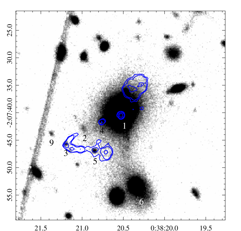
Figure 1.— Central field of the Gemini pre-image. Objects are labeled with the slit number. The image shows the central $\sim 40\times 40$ arcsec of the field. Blue contours show the 5 GHz VLA map of Morganti et al. (1999). Object with label 4 is identified as S3.7 in Massaro et al. (2009). Note that the radio jet reignites “after” object 2, as shown in Figure 3 of Massaro et al. (2009). The jet sharply bends after object 3 which corresponds to object S11.3 in the Massaro et al. (2009) nomenclature. The straight line across the image is a satellite trail, also visible in Figure 2. North is up and East is left.

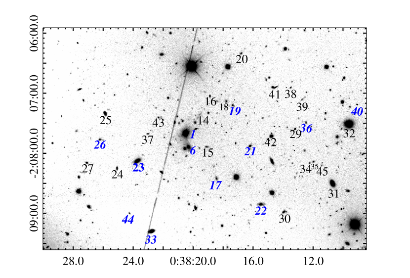
Figure 2.— GMOS $r^{\prime}$-band image centered on 3C 17. Galaxies selected for spectroscopy are labeled with the slit number. Cluster members are indicated in blue, italic font. 3C 17 is labelled with number 1. North is up and east is left.

Table 1Targets of the GMOS multislit mask

Slit	R.A.	Decl.	z	m${}_{r^{\prime}}$	Comments
1*	00:38:20.529	-02:07:40.29	0.221	17.84	3C 17
2	00:38:20.976	-02:07:42.51	—	24.39	Linear object
3	00:38:21.197	-02:07:45.72	—	24.06	S11.3
4	00:38:20.762	-02:07:41.40	—	24.47	S3.7
5	00:38:20.847	-02:07:46.99	—	24.14	knot
6*	00:38:20.351	-02:07:53.41	0.220	19.35	2nd brightest galaxy
7	00:38:19.841	-02:07:53.41	—	—	sky
8	00:38:21.586	-02:07:41.40	—	—	sky
9	00:38:21.374	-02:07:43.86	—	24.15	knot
10	00:38:20.069	-02:07:40.29	—	—	sky
11	00:38:21.828	-02:07:42.51	—	—	sky
12	00:38:22.102	-02:07:45.72	—	—	sky
13	00:38:21.672	-02:07:46.99	—	—	sky
14	00:38:19.624	-02:07:21.49	—	22.18	Interacting
15	00:38:19.115	-02:07:53.57	0.275	21.65	Spiral
16	00:38:18.923	-02:07:02.83	0.799	21.71	Irregular
17*	00:38:18.475	-02:08:25.22	0.226	21.32	Spiral
18	00:38:17.814	-02:07:07.95	—	21.72	Elliptical
19*	00:38:17.401	-02:07:11.97	0.222	21.77	Elliptical
20	00:38:16.820	-02:06:20.21	0.670	21.74	Barred
21*	00:38:16.236	-02:07:52.66	0.221	20.71	Elliptical
22*	00:38:15.495	-02:08:50.91	0.212	20.30	Spiral-Interacting
23*	00:38:23.754	-02:08:07.66	0.222	18.48	S0
24	00:38:25.115	-02:08:14.57	0.421	20.89	Irregular
25	00:38:25.920	-02:07:20.17	0.165	20.54	Spiral-Interacting
26*	00:38:26.252	-02:07:46.41	0.221	21.16	Elliptical-Interacting
27	00:38:27.128	-02:08:09.73	0.477	20.90	Elliptical?
28	00:38:28.817	-02:07:22.91	0.160	22.90	Elliptical
29	00:38:13.241	-02:07:35.93	0.410	21.43	Elliptical
30	00:38:13.984	-02:08:58.44	0.255	20.93	Irregular
31	00:38:10.744	-02:08:30.05	0.112	18.79	Barred-Spiral
32	00:38:09.633	-02:07:30.86	0.058	18.02	Spiral
33*	00:38:22.805	-02:09:18.00	0.217	19.37	Spiral
34	00:38:12.265	-02:08:09.84	0.398	22.52	Elliptical
35	00:38:11.998	-02:08:08.38	0.402	22.20	Elliptical
36*	00:38:12.511	-02:07:29.30	0.220	22.04	Elliptical
37	00:38:23.054	-02:07:40.65	0.321	22.46	Spiral
38	00:38:13.516	-02:06:54.34	0.367	22.25	Spiral
39	00:38:12.761	-02:07:06.50	—	22.62	Spiral
40*	00:38:09.092	-02:07:11.21	0.217	22.35	Elliptical
41	00:38:14.551	-02:06:54.36	0.671	21.82	Spiral-Interacting
42	00:38:15.074	-02:07:45.89	0.463	23.01	Elliptical
43	00:38:22.341	-02:07:24.30	0.320	22.05	Elliptical
44*	00:38:24.276	-02:07:59.99	0.218	22.55	Irregular
45	00:38:11.458	-02:08:12.18	—	22.98	Irregular

Note. — Column 1: slit number, an asterisk denotes cluster membership. Column 2: Right Ascension (J2000). Column 3: Declination (J2000). Column 4: redshift. Column 5: apparent $r^{\prime}$ magnitude. Column 6: Comments. While most of the spectroscopic targets are uncataloged the following objects have other names: slit 23: GALEXMSC J003823.80-020811.3; slit 32: GALEXASC J003809.60-020731.7; slit 33: GALEXMSC J003822.72-020917.6; slit 41: GALEXMSC J003823.80-020654.2

2.1. Data Reduction

Standard data reduction is carried out with the Gemini IRAF package. A summary of our data reduction procedures can be found in Madrid & Donzelli (2013), Muriel et al. (2015), and Rovero et al. (2016). In the following paragraphs we describe the most important steps of the data reduction.

Images are pre-processed through the standard Gemini pipeline that corrects for bias, dark current, and flat-field. Spectral data are processed with the gsreduce task, which performs overscan, and cosmic ray removal. Bias and flat-field frames are generated with the gbias and gsflat routines. The sky level is removed interactively using the task gskysub, and each of the spectra are extracted with the gsextract routine. Wavelength calibration is performed using the task gswavelength, while flux calibration is done with the gscalibrate routine, which uses the sensitivity function derived by the gsstandard task. For this purpose, the spectra of the spectrophotometric standard star $g191$ were taken with an identical instrument configuration. The photometric zero-point is taken from the Gemini website .

Redshifts are derived using the fxcor routine of IRAF on the continuum-subtracted spectra. This task computes radial velocities by deriving the Fourier cross correlation between two spectra. The spectra for globular clusters and planetary nebulae in NGC 7793, obtained during a previous Gemini run, are used as templates. Redshifts are computed using four or more of the following lines: H$\beta$, [O III] (4959, 5007Å), H$\alpha$, [N II] (6583Å), and the Mg I and Na absorption lines. Target coordinates, magnitudes, and redshifts are listed in Table 1. The largest error on the redshifts given by the task fxcor is 0.001, hence the number of significant digits reported in Table 1. Photometric measurements are carried out using the Gemini pre-image and are explained in section 6.

3. A cluster detection at the 3C 17 redshift

Figure 3 shows the redshift distribution of the 31 galaxies for which a redshift is measured. There is a conspicuous cluster at $z\sim 0.2$ consisting of 12 galaxies, including 3C 17. The number of cluster members should be taken as a lower threshold given that many galaxies in the field of view have magnitudes that are in the range of those measured for cluster members but were not included in the GMOS mask. Also, Figures 1 and 2 show that there is a concentration, or overdensity, of galaxies toward 3C 17. Some of these galaxies show clear signs of interactions, such as tidal tails and plumes. There is a clear bridge between 3C 17 and a companion galaxy to the south noted earlier by Ramos Almeida (2011).

Figure 4 shows the Gemini spectra for the members of the 3C 17 galaxy cluster that have emission lines. Figure 5 shows the spectra for cluster members identified through their absorption lines.

Table 1 contains the position and object description for all slits in the GMOS mask. It also contains the redshift and magnitudes for those targets that have these two quantities determined.

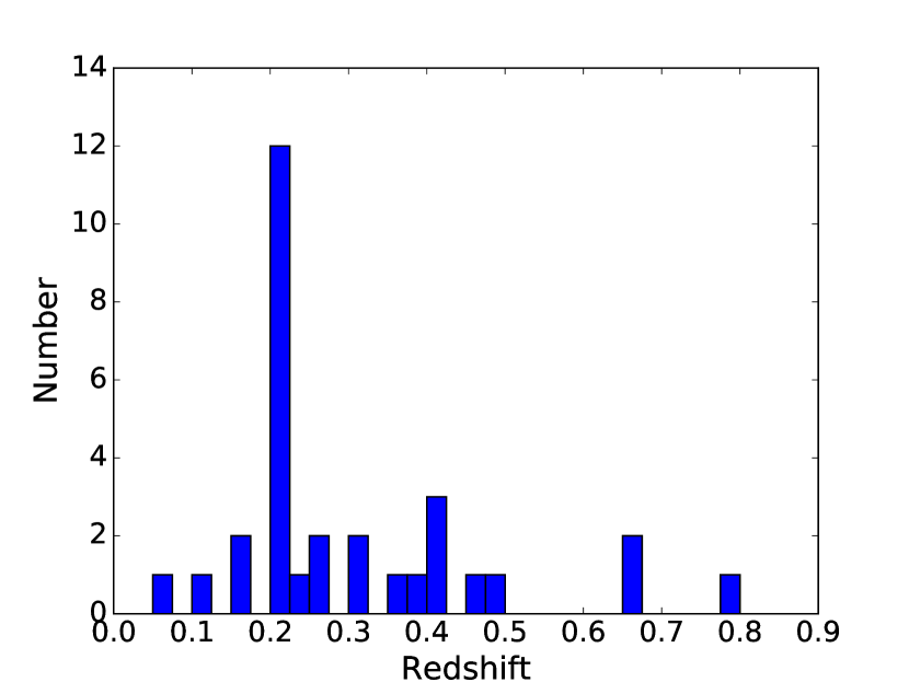
Figure 3.— Redshift distribution for target galaxies. A conspicuous cluster of twelve galaxies is present at $z$=0.2

The mean redshift ($z_{mean}$) and the velocity dispersion ($\sigma_{v}$) of this galaxy cluster are derived using the Gapper estimator as defined in Beers et al. (1990). An example of the application of this method can be found in Muriel et al. (2015).

For the 3C 17 cluster, the mean redshift is $z_{mean}=0.220\pm 0.003$, and its velocity dispersion $\sigma_{v}=821~{}\pm~{}171$ km s^-1. The virial radius is computed using the harmonic mean of the projected separations between the cluster members (see formula (1) given in Section 3.3 by Nurmi et al. (2013)), which yields $R_{vir}=0.37$ Mpc. These values suggest a cluster of galaxies (e.g. Amodeo et al., 2017).

4. 3C 17 Jet knots

The comparison between radio and X-ray emission in the curved jet of 3C 17 was originally carried out by Massaro et al. (2009) to highlight jet knots with X-ray counterparts. Two of these X-ray knots, S3.7 and S11.3, are particularly interesting because they also have optical counterparts (which correspond in Fig. 1 to slits 4 and 3, respectively). Even more intriguing is the fact that the jet sharply bends after one of these knots, S11.3 (slit 3 in Figure 1). Some of these knots are also present in the near infrared image of Inskip et al. (2010).

Slits are placed on each of these aforementioned knots in an effort to determine their nature. Figure 1 shows a zoomed-in view of the central region around 3C 17 with objects selected for spectroscopy. Emission lines are not detected for knots 2, 3, 4, 5, and 9. The Gemini data place an upper limit of $10^{-18}$ erg cm^-2 s^-1 Å^-1 for the flux of any potential emission line present on the jet knots described above.

The absence of detectable emission lines for slit 2, in particular, is relevant. The object labeled 2 in Figure 1 is roughly perpendicular, in projection, to the path of the jet; see also the HST image presented by Massaro et al. (2009). A plausible explanation for the nature of this object is an emitting region that arises from the interaction of the jet with a gas cloud (e. g. H i), which is shock-ionized by the jet and produces free-free emission (Massaro et al., 2009). The absence of emission lines weakens the possible presence of shocks.

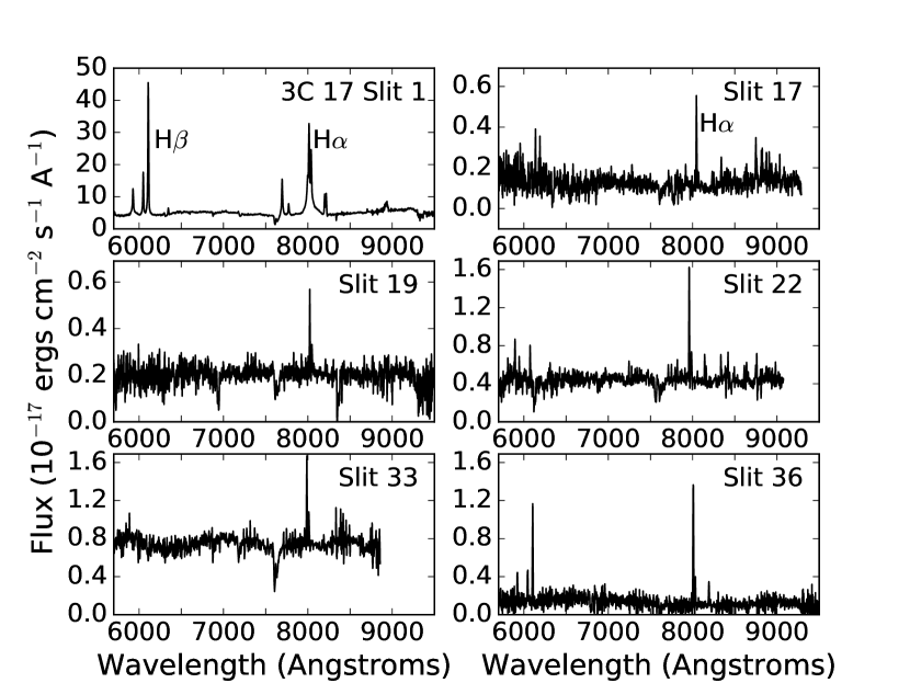
Figure 4.— Spectra for the cluster galaxies with emission lines. These spectra are shown at their observed wavelength; that is, they are not corrected for radial velocities. The prominent emission line at 8006 Å is H$\alpha$.

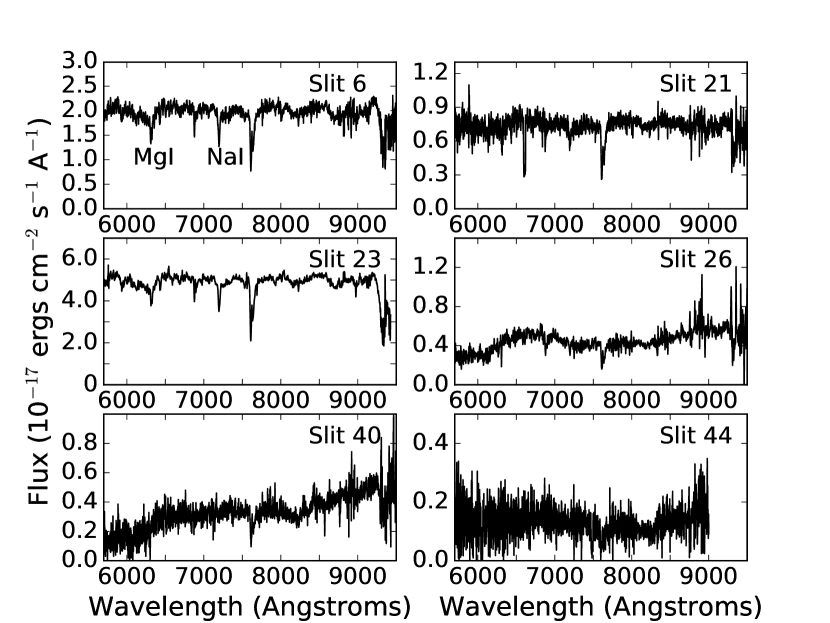
Figure 5.— Spectra for the cluster galaxies identified by their absorption lines. These spectra are not corrected for radial velocities. The prominent absorption feature at 7610 Å is a telluric line.

5. The Spectrum of 3C 17

The optical spectrum of 3C 17 is also obtained with the new Gemini data. An analysis of this spectrum is given in this section. In order to study the physics of the ionized gas in the 3C 17 core, it is first necessary to correct the data for Galactic extinction. Here, a value of E(B-V) = 0.023 mag is adopted, as determined by Schlafly & Finkbeiner (2011). The presence of H$\alpha$ and H$\beta$ also allow us to assess the extinction affecting the Narrow-Line Region (NLR). For this purpose, an intrinsic Balmer decrement of 3.1, typical of AGNs (Osterbrock, 1989), is assumed. The observed narrow emission-line flux ratio of H$\alpha$/H$\beta$ = 3.15 indicates that the amount of dust in the line of sight of the NLR is negligible.

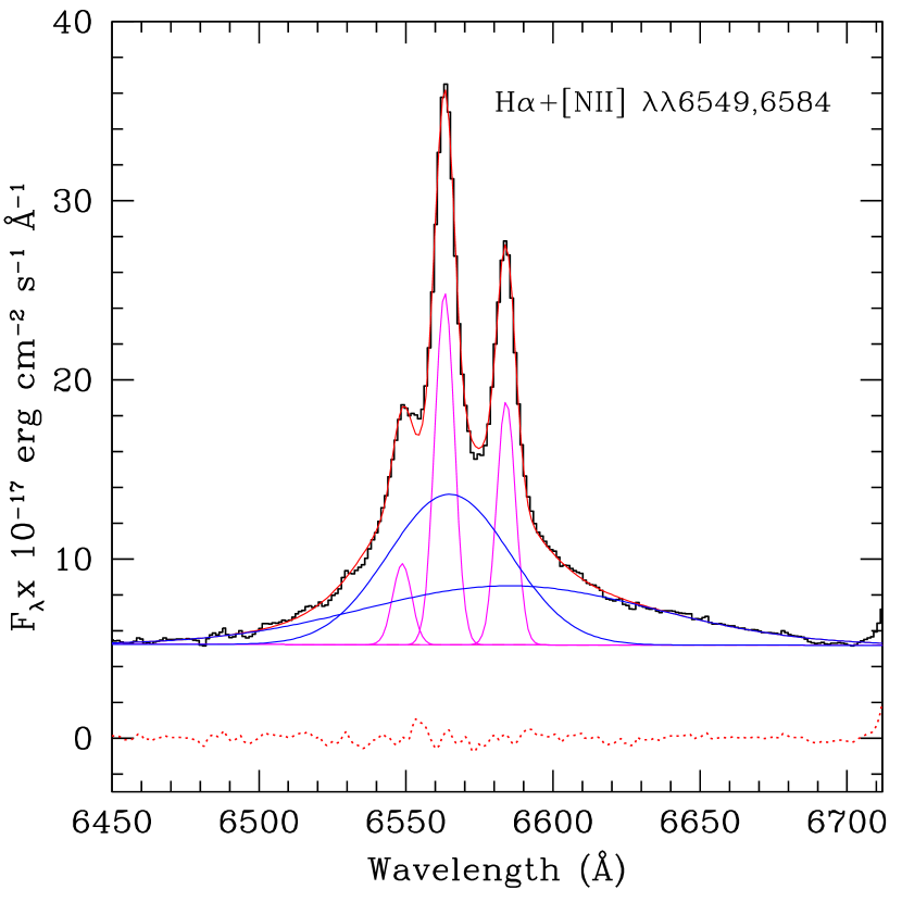
Figure 6.— Example of the deblending procedure applied to H$\alpha$. The black histogram line is the observed spectrum, and the total fit is in red. The dashed line is the residual after subtraction of the fit. Components associated with the NLR are in magenta, while those associated with the BLR are in blue. Note that the redshifted H$\alpha$ emission is observed at 8006 Å; see Figure 1.

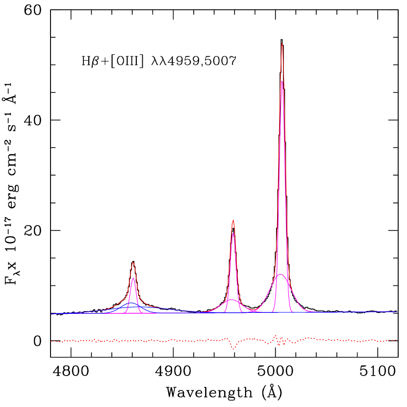
Figure 7.— Same as Fig. 6 but for H$\beta$.

The optical spectrum extracted from the nuclear region of 3C 17 is dominated by prominent emission lines of H$\alpha$+[N ii], H$\beta$, and [O iii] on top of a continuum with evidence of stellar absorption features. The base of the Balmer lines shows the presence of broad components, confirming that this source is a broad-line object (BLO) as suggested by Baldi et al. (2013). Low-ionization narrow emission lines of [S ii] $\lambda\lambda$6717, 6731, and [O i] $\lambda\lambda$6300, 6363 are also conspicuous in the spectrum. The redshift derived from the position of these lines is $z=0.220\pm 0.001$, in very good agreement with recent values found in the literature for this object (Buttiglione et al., 2010; Baldi et al., 2013).

Emission-line fluxes on the 3C 17 spectrum are measured using the LINER routine (Pogge & Owen, 1993), a $\chi$-squared minimization algorithm that can fit simultaneously up to eight profile functions to a given line or set of blended lines. In all cases, the underlying continuum was fit by a low-order polynomial. LINER also provides values for the peak position and the full width at half-maximum (FWHM) of each profile function. The number of Gaussian components fit varied depending on the emission line. In order to deblend the broad and narrow components of H$\alpha$ and H$\beta$, three Gaussian profiles were necessary for each line (see below). Figures 6 and 7 show examples of the deblending procedure for the spectral regions containing H$\alpha$ and H$\beta$. Column 4 of Table 2 lists the emission-line fluxes measured in the spectrum of 3C 17.

Table 23C 17 Emission Lines

H$\alpha_{n}$ & 6563.1 351 164
H$\alpha_{b}$ 6564.8 2223 435
H$\alpha_{vb}$ 6585.2 5326 409
$[$N II$]$ 6584.1 341 110
$[$S II$]$ 6717.1 366 61
$[$S II$]$ 6731.5 365 64
$[$O I$]$_n 6300.4 356 70
$[$O I$]$_i 6301.8 1016 87
H$\beta_{n}$ 4860.6 430 52
H$\beta_{b}$ 4861.6 2218 75
H$\beta_{vb}$ 4876.6 5225 61
$[$O III$]$_n 5006.6 381 296
$[$O III$]$_i 5004.9 1435 178
HeII 4684.0 440 10

Note. — The subscript $n$ stands for narrow component; likewise, $i$ stands for intermediate; $b$ for broad; and $vb$ is for very broad.

Column 3 of Table 2 displays the values of FWHM found from the fit. These values are already corrected in quadrature by an instrumental broadening of 73 km s^-1, measured from the sky lines present in the spectra and CuAr frames obtained for wavelength calibration.

The narrow component of H$\alpha$ has a FWHM of 351$\pm$10 km s^-1 in velocity space, compatible with an origin in the NLR of 3C 17. The forbidden lines of [N ii], [S ii], [O i], and [O iii] have similar FWHMs. Note that in the latter two lines we also found the presence of an intermediate component, associated with the NLR, with FWHMs of 1016 km s^-1 and 1435 km s^-1, respectively. These lines are labeled with the subscript $i$ in Table 2. In the case of [O iii], the centroid of that component is blueshifted by 120 km s^-1 relative to that of the narrower component.

We associate this blueshifted [O iii] emission with outflowing gas. Indeed, blue asymmetries in this line are usually indicative of nuclear outflows (Komossa et al., 2008; Zakamska et al., 2016; Marziani et al., 2016). The fact that the slit in 3C 17 was positioned along the radio jet supports this scenario. The presence of a broader component in [O i] is most likely due to a strong blend with [S iii] $\lambda$6312, as such a component is not present in [O i] $\lambda$6363. [S iii] $\lambda$6312 is a forbidden line, observed in narrow line regions and used to determine gas temperature (Contini & Viegas, 1992).

The presence of a broad-line region in 3C 17 is clearly manifested by the detection of two broad components in the Balmer lines with FWHMs of 2220$\pm$30 km s^-1 and 5300$\pm$90 km ^-1 (marked in Table 2 with the subscripts $b$ and $vb$, for broad and very broad components, respectively). While these peaks are very close in position with the rest-wavelength expected for H$\alpha$ and H$\beta$ ($\leq$ 2 Å), the latter is significantly redshifted, with the peak located $\sim$1000 km s^-1 relative to the narrow component of that line. Hints of broad wings for the H$\beta$ line were reported earlier by Tadhunter et al. (1993).

In optical spectroscopy, host galaxies with broad emission lines significantly Doppler-shifted from the corresponding narrow lines have been interpreted as the consequence of a late-stage supermassive black hole (SMBH) merger, or, alternatively, due to a kick received by the broad-lined SMBH resulting from anisotropic gravitational emission (Popovic, 2012; Komossa et al., 2012). In the case of 3C 17, the velocity shift of the very broad component and the narrow component amounts to $\sim$1000 km s^-1. This value is well within the expected range of velocity separation between the narrow and broad components predicted in both scenarios above (Campanelli et al., 2007).

6. Photometric measurements

Total magnitudes for the 39 spectroscopic targets are derived using aperture photometry on the Gemini pre-image. Photometric measurements are obtained with the task phot within IRAF daophot. Total magnitudes are obtained by fitting a series of concentric circular diaphragms until the total flux converged. Sky fitting and background subtraction are carried out around each object, attentively avoiding stars and neighboring objects. The magnitude for 3C 17 is derived by fitting a surface brightness profile as described below. Total magnitudes are listed in Table 1. Considering that the mean redshift to the cluster is $z=0.220$, the brightest cluster galaxy (BCG) 3C 17 has an absolute magnitude of M_r = -22.45 mag. The second brightest galaxy corresponds to slit 23 and it has an absolute magnitude of M_r = -21.52 mag.

Figure 8.— Luminosity profile of 3C 17. Upper panel shows the Sérsic + exponential fit, while the lower pannel shows the exponential + Sérsic fit.

Table 3Parameters of the 3C 17 Surface Brightness Profile

Obj. + fit	$\mu_{e}$	$r_{e}$	$n$	$\mu_{0}$	$r_{0}$	$M_{r^{\prime}}$	chi-sq	rms
		kpc			kpc
3c 17 (S+E)	18.06	0.9	5.04	22.93	13.9	-22.45	21	9
3c 17 (E+S)	25.76	40.5	4.90	18.61	1.2	…	5	4

Note. — Column (1): object and fit type, Sérsic plus exponential (E+S), or exponential plus Sérsic (E+S); column (2): effective surface magnitude; column (3): effective radius (kpc); column (4): $n$ parameter; column (5): central surface magnitude; column (6): scale length (kpc); column (7): Absolute r’ magnitude; column (8): chi-sq parameter; column (9): rms.

6.1. The Luminosity profile of 3C 17

The luminosity profile for 3C 17 is analyzed following the methods described in Donzelli et al. (2011) and Madrid & Donzelli (2016). In summary, the galaxy light profile is extracted using the ellipse routine (Jedrzejewski, 1987) of the Space Telescope Science Analysis System (STSDAS) package. For 3C 17, galaxy overlapping is an issue that we circumvent by applying the technique described in Coenda et al. (2005). This technique consists of masking all overlapping galaxies before profile extraction and constructing a model of the target galaxy using its luminosity profile. This model is then subtracted from the original image and the resulting residual image is used to isolate the profile of overlapping galaxies. We iterate this process until the profile of the target galaxy converges.

The Sérsic profile (Sérsic, 1968),

$$I(r)=I_{e}\exp\Big{\{}-b_{n}\Big{[}\Big{(}\frac{r}{r}_{e}\Big{)}^{\beta}-1\Big{]}\Big{\}}$$ (1)

is used for surface brightness profile fitting. In the expression of the Sérsic profile given above, $I_{e}$ is the intensity at $r=r_{e}$, the radius that encloses half of the total luminosity, and $b_{n}$ can be calculated using $b_{n}\sim 2\/n-0.33$, and $\beta=1/n$ (Caon et al., 1993).

Profile fitting is done with the nfit1d routine within STSDAS. This task uses a $\chi^{2}$ minimization scheme to fit the best nonlinear functions to the galaxy light profile. Isophote fitting is performed down to a count level of 2$\sigma_{sky}$ that corresponds to a surface magnitude of $\mu_{r}\sim$25.5 mag/arcsec^-2.

For 3C 17 a single Sérsic model fails to properly fit the luminosity profile. It is then necessary to add an outer exponential function (Freeman et al., 1970):

$$I(r)=I_{0}\exp\Big{(}-\frac{r}{r}_{0}\Big{)}$$ (2)

In the equation above, $I_{0}$ is the central intensity and $r_{0}$ is the scale length. As suggested by Donzelli et al. (2011), this exponential component is the simplest function to account for the ‘extra-light’ observed in many Brightest Cluster Galaxies galaxies. The necessity of including an outer component on the surface brightness modeling is due to the extended envelopes common of BCGs. The extra exponential required to fit the brightness profile of 3C 17 suggests that this galaxy is a typical BCG. The most accurate fit for the light profiles of BCGs is indeed a two component model, with an inner and outer component (e.g. Gonzalez et al., 2005; Seigar al., 2007; Donzelli et al., 2011). The fact that the host galaxy of 3C 17 is a BCG gives further support to the binary SMBH merger hypothesis, discussed in Section 5, as the likely evolutionary scenario to give rise to broad emission lines Doppler-shifted from the corresponding narrow lines. Corroboration of this hypothesis would require long-term monitoring.

Figure 8 shows the luminosity profile for 3C 17 together with the fitting functions. The upper panels show the classic Sérsic plus exponential fit, while the lower panels show the exponential plus Sérsic fit. Fitting parameters are shown in Table 3. Taking a look at the chi-squared and rms coefficients from this table we can also compare the quality of both types of fit. It is clear that, at least from a mathematical point of view, the inner exponential plus Sérsic fit gives a better fit to the luminosity profile than the classical Sérsic $+$ outer exponential.

7. X-Ray data

Figure 9.— Background-subtracted, exposure-weighted surface brightness profiles in the $0.5-2\mbox{ keV}$ band (left panel) and $0.5-7\mbox{ keV}$ band (right panel) extracted in the NE-SW direction (see the main text). The widths of the bins are adaptively chosen to reach a minimum signal-to-noise ratio of 3.

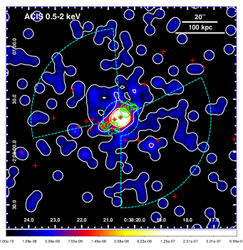
Figure 10.— Broadband $0.5-2\text{keV}$ (left panel) and $0.5-7\text{keV}$ (right panel) ACIS-S flux images centered on 3C 17. These two images are smoothed with a $8\times 8$ pixel ($3.94\arcsec\times 3.94\arcsec$) gaussian kernel. The green contours are from the 5 GHz VLA map of Morganti et al. (1999) with a restoring beam of $0.\arcsec 4\times 0.\arcsec 4$, the white lines are the contours of the X-ray flux image, and the red crosses indicate the galaxies in the field. The cyan dashed cones are the regions used for the extraction of the surface brightness profiles, with the last bin where the signal-to-noise ratio is at least three extending up to $\sim$50$\arcsec$.

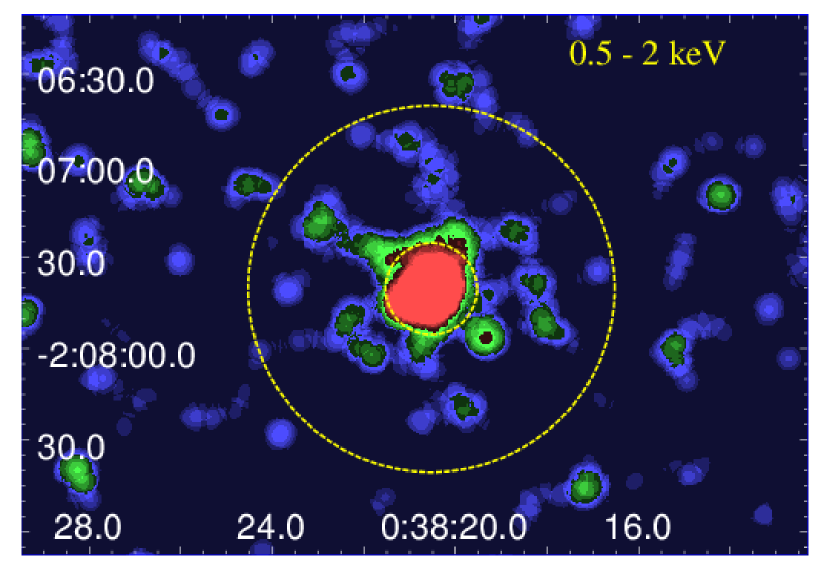
Figure 11.— Chandra broadband $0.5-2\text{keV}$ image smoothed with a Gaussian kernel of 16 pixels. This image shows the annulus (dotted yellow lines) where the emission emanating from the ICM is measured. Note that this image has a bigger field of view than the images shown in Figure 10.

Chandra data are retrieved from the Chandra Data Archive through the ChaSeR service. Archival data consist of a $8.0$ ks observation (9292, PI: Harris, GO 9) performed in February 2008 in VFAINT mode. These data are analyzed with the CIAO data analysis system (version 4.9; Fruscione et al., 2006) and Chandra calibration database CALDB version 4.7.6, adopting standard procedures.

Figure 9 features two broadband, $0.5-2$ and $0.5-7$ keV Chandra images centered on ACIS-S chip 7. Point-spread function (PSF), exposure, and flux maps are produced using the task mkpsfmap. PSF and exposure maps are used to detect point sources in the $0.5-7$ keV energy band with the wavdetect tool, adopting a $\sqrt{2}$ sequence of wavelet scales (i.e., 1, 2, 4, 8, 16, and 32 pixels) and a false-positive probability threshold of ${10}^{-6}$.

To estimate the background emission we use blank-sky data included in the Chandra CALDB and re-projected to the same tangent plane of the observation. We then produce background event files for each ACIS chip, and rescale them to match the observation count rate in the $9-12\mbox{ keV}$ band.

To evaluate the physical scale of the X-ray emission we extract background-subtracted, exposure-weighted surface brightness profiles from the source-removed event files, shown in Fig. 10. The widths of the bins are adaptively determined to reach a minimum signal-to-noise ratio of three. For this analysis we choose the directions between PAs 15^∘ and 103^∘, and between 180^∘ and 297^∘, in order to avoid the emission observed in the radio in the GHz range. We also exclude the inner (10$\arcsec$) since this observation is affected by severe pile-up, as shown in the map produced with the pileup_map tool.

We find that in the $0.5-7$ keV band the last bin that reaches a signal-to-noise ratio of 3 extends up to $51\arcsec$. This extended X-ray emission, mainly in the soft $0.5-2\text{keV}$ band, could be due to the presence of hot gas in the intergalactic medium. We measure the X-ray flux in an annulus between 5 arcsec (inner radius) and 60 arcsec (outer radius) from the nucleus of 3C 17; we thus exclude the contribution from the AGN, as shown in Figure 11. The flux measured for this annulus is $3.84\pm 2.55\times 10^{-14}$ in cgs units ($10^{-15}$ erg cm^-2 s^-1). This is the integrated flux in the 0.5-2 keV energy range, where most of the diffuse X-ray emission due to the ICM is expected. The X-ray flux above yields an ICM X-ray luminosity of $L_{X}=5.77\pm 3.83\ \times 10^{42}$ erg/s.

The reason why the 3C 17 jet sharply bends is better understood with the identification of a cluster of galaxies. Indeed, the jet emitted by 3C 17 propagates through a dense intracluster medium. Bent-tail galaxies, or radio-loud AGN with jets that bend as they propagate through the dense ICM, have been reported at high redshift. For instance, Blanton et al. (2003) discovered a cluster of galaxies, at $z$=0.96, using a combination of VLA imaging and Keck spectroscopy. 3C 17 also has an extended radio emission detected at 5 GHz with the VLA (Morganti et al., 1993) although it appears to have a smaller spatial scale than the diffuse X-ray emission.

8. Final remarks

An optical and X-ray study of 3C 17 and its environment was carried out using Gemini and Chandra data. The presence of a strikingly curved radio jet and several unclassified sources along the path of the jet are principal motivations for this study. The main findings of this work are as follows:

• 3C 17 is part of a galaxy cluster at a redshift of $z=0.220\pm 0.003$. Twelve cluster members have their redshifts determined with Gemini spectra.

• The velocity dispersion of these 12 members is $\sigma_{v}=821~{}\pm~{}171$ km s^-1, consistent with the velocity dispersion of a cluster of galaxies.

• The spectrum of 3C 17 is dominated by broad emission lines.

• 3C 17 is the brightest cluster member. The 3C 17 surface brightness profile is best fit with a double component model characteristic of BCGs.

• The analysis of the surface brightness profiles of archival Chandra data reveals the presence of extended soft X-ray emission surrounding 3C 17 that is likely to originate in the hot gas of the intergalactic medium.

Properly characterizing the environment of AGNs with bent jets is relevant given that these radio sources are often used as tracers of high-redshift clusters (e.g. Blanton et al., 2000; Wing & Blanton, 2011; Paterno-Mahler et al., 2017). Bent-tail radio galaxies will also be used as signposts for distant galaxy clusters in future wide-field radio-continuum surveys, e. g. the Evolutionary Map of the Universe (EMU) to be carried out with the Australian Square Kilometer Array Pathfinder (Norris et al., 2013).

References

- Amodeo et al. (2017) Amodeo, S., Mei, S., Stanford, S. A., et al. 2017, ApJ, 844, 101
- Baldi et al. (2013) Baldi, R. D., Capetti, A., Buttiglione, S., Chiaberge, M. & Celotti, A. 2013, A&A, 560, 81
- Balmaverde et al. (2012) Balmaverde, B., Capetti, A., Grandi, P., Torresi, E., et al. 2012, A&A, 545, 143
- Begelman et al. (1979) Begelman, M. C., Rees, M. J. & Blandford, R. D. 1979, Nature, 279, 770
- Bennett et al. (1962a) Bennett, A. S. 1962a, MmRAS, 68, 163
- Bennett et al. (1962b) Bennett, A. S. 1962b, MNRAS, 125, 75
- Blanton et al. (2000) Blanton, E., Gregg, M. D., Helfand, D. J., et al. 2000, ApJ, 531, 118
- Blanton et al. (2003) Blanton, E., Gregg, M. D., Helfand, D. J., et al. 2003, AJ, 125, 1635
- Buttiglione et al. (2010) Buttiglione, S., Capetti, A., Celotti, A., et al. 2010, A&A 509, 6
- Beers et al. (1990) Beers, T.C., Flynn, K. & Gebhardt, K. 1990, AJ, 100,32
- Campanelli et al. (2007) Campanelli, M., Lousto, C., Zlochower, Y., Merritt, D. 2007, ApJL, 659, L5
- Caon et al. (1993) Caon, N., Capaccioli, M., & D’Onofrio, M. 1993, MNRAS, 265, 1013
- Cleary et al. (2007) Cleary, K., Lawrence, C. R., Marshall, J. A., et al. 2007, ApJ, 660, 117
- Coenda et al. (2005) Coenda, V., Donzelli, C.J., Muriel, H., Quintana, H., Infante, L. 2005, AJ, 129, 1237
- Contini & Viegas (1992) Contini, M. & Viegas, S. M. 1992, ApJ, 401, 481
- de Koff et al. (1996) de Koff, S., Baum, S. A., Sparks, W. B., et al. 1996, ApJS, 107,621
- Donzelli et al. (2011) Donzelli, C.J., Muriel, H., & Madrid, J. P. 2011, ApJ, 195, 15
- Edge et al. (1959) Edge, D. O., Shakeshaft, J. R., McAdam, W. B., Baldwin, J. E., & Archer, S. 1959, Mem. R. Astron. Soc., 68, 37
- Evans et al. (2006) Evans, D. A., Worrall, D. M., Hardcastle, M. J., Kraft, R. P., Birkinshaw, M. 2006, ApJ, 642, 96
- Freeman et al. (1970) Freeman, K. C. 1970, ApJ, 160, 811
- Fruscione et al. (2006) Fruscione, A., McDowell, J. C., Allen, G. E., et al. 2006, Proc. SPIE, 6270, 62701V
- Gisler & Miley (1979) Gisler G. R. & Miley, G. K. 1979, A&A, 76, 109
- Gonzalez et al. (2005) Gonzalez, A. H., Zabludoff, A. I., & Zaritsky, D. 2005, ApJ,618, 195
- Gunn et al. (1981) Gunn, J. E., Hoessel, J. G., Westphal, J. A., Perryman, M. A. C. & Longair, M. S. 1981, MNRAS, 194, 111
- Hardcastle & Worrall (2000) Hardcastle, M. J. & Worrall, D. M. 2000, MNRAS, 319, 562
- Inskip et al. (2010) Inskip, K. J., Tadhunter, C. N., Morganti, R., et al. 2010, MNRAS, 407, 1739
- Jedrzejewski (1987) Jedrzejewski, R. 1987, MNRAS, 226, 747
- Komossa et al. (2008) Komossa, S., Xu, D., Zhou, H., Storchi-Bergmann, T., Binette, L. 2008, ApJ, 680, 926
- Komossa et al. (2012) Komossa, S. 2012, Advances in Astronomy, 2012, 364973
- Kristian et al. (1974) Kristian, J., Sandage, A. & Katem, B. 1974, ApJ, 191, 43
- Laing et al. (1983) Laing, R. A., Riley, J. M. & Longair, M. S. 1983, MNRAS, 204, 151
- Leipski et al. (2010) Leipski, C., Haas, M., Willner, S. P. et al. 2010, ApJ, 717, 766
- Lynden-Bell (1969) Lynden-Bell, D. 1969, Nature, 223, 690
- Madrid et al. (2006) Madrid, J. P., Chiaberge, M., Floyd, D. et al. 2006, ApJS, 164, 307
- Madrid & Donzelli (2013) Madrid, J. P. & Donzelli, C. J. 2013, ApJ, 770, 158
- Madrid & Donzelli (2016) Madrid, J. P. & Donzelli, C. J. 2016, ApJ, 819, 50
- Martel et al. (1999) Martel, A. R., Baum, S. A., Sparks, W. et al. 1999, ApJS, 122, 81
- Marziani et al. (2016) Marziani, P., Sulentic, J. W., Stirpe, G. M., et al. 2016, Astrophysics and Space Science, 361, 3
- Maselli et al. (2016) Maselli, A., Massaro, F., Cusumano, G., et al. 2016, MNRAS, 460, 3829
- Massaro et al. (2009) Massaro, F., Harris, D. E., Chiaberge, M., et al. 2009, ApJ, 696, 980
- Massaro et al. (2010) Massaro, F., Harris, D. E., Tremblay, G. R. et al. 2010, ApJ, 714, 589
- Massaro et al. (2012) Massaro, F., Tremblay, G. R., Harris, D. E., et al. 2012, ApJS, 203, 31
- Massaro et al. (2013) Massaro, F., Harris, D. E., Tremblay, G. R., et al. 2013, ApJS, 206, 7
- Massaro et al. (2015) Massaro, F., Harris, D. E., Liuzzo, E., et al. 2015, ApJS, 220, 5
- Massaro et al. (2018) Massaro, F., Missaglia, V., Stuardi, C., et al. 2018, ApJS, 234, 7
- McCarthy et al. (1997) McCarthy, P., Miley, G. K., de Koff, S. et al. 1997, ApJS, 112, 415
- Morganti et al. (1999) Morganti, R., Oosterloo, T., Tadhunter, C. N., et al. 1999, Astronomy & Astrophysics Supplement, 140, 355
- Morganti et al. (1993) Morganti, R., Killeen, N. E. B., Tadhunter, C. N. 1993, MNRAS, 263, 1023
- Muriel et al. (2015) Muriel, H., Donzelli, C. J., Rovero, A. C. & Pichel, A. 2015, A&A, 574, A101
- Norris et al. (2013) Norris, R. P., Hopkins, A. M., Afonso, J., et al. 2013, PASA, 30, 20
- Nurmi et al. (2013) Nurmi, P., Heinämäki, P., Sepp, T., et al. 2013, MNRAS, 436 380
- O’Dea & Owen (1986) O’Dea, C. P. & Owen, F. N. 1986, ApJ, 301, 841
- Osterbrock (1989) Osterbrock D. E. 1989 The Astrophysics of Gaseous Nebulae and Active Galactic Nuclei (Mill Valley, CA: Univ. Science Books)
- Paterno-Mahler et al. (2017) Paterno-Mahler, R., Blanton, E. L., Brodwin, M., et al. 2017, ApJ, 844, 78
- Planck Collaboration (2016) Planck Collaboration XIII, 2016, A&A, 594, 13
- Pogge & Owen (1993) Pogge, R. W., & Owen, J. M. 1993, LINER; An Interactive Spectral Line Analysis Program, OSU Internal Report 93-01
- Popovic (2012) Popovic, L. Č. 2012, New Astr. Rev. 56, 74
- Ramos Almeida (2011) Ramos Almeida, C., Tadhunter, C. N., Inskip, K. J., et al. 2011, MNRAS, 410, 1550
- Rovero et al. (2016) Rovero, A.C., Muriel, H., Donzelli, C.J. & Pichel, A. 2016, A&A, 589, 92
- Salpeter (1964) Salpeter, E. E. 1964, ApJ, 140, 796
- Schlafly & Finkbeiner (2011) Schlafly, E., & Finkbeiner, D. P. 2011, ApJ, 737, 103
- Schmidt (1965) Schmidt, M. 1965, ApJ, 141, 1
- Seigar al. (2007) Seigar, M. S., Graham, A. W., & Jerjen, H. 2007, MNRAS, 378, 1575
- Sérsic (1968) Sérsic, J. L. 1968, Atlas de Galaxias Australes, Córdoba, Argentina: Observatorio Astronómico, 1968
- Sijbring & Bruyn (1998) Sijbring, D. & de Bruyn, A. G. 1998, A&A, 331, 901
- Smith & Spinrad (1988) Smith, H. E. & Spinrad, H. 1980, PASP, 92, 553
- Spinrad & Djorgovski (1984) Spinrad, H. & Djorgovski, S. 1984, ApJ Letters, 285, L49
- Spinrad et al. (1985) Spinrad, H., Marr, J., & Aguilar, L., Djorgovski, S. 1985, PASP, 97, 932
- Stuardi et al. (2018) Stuardi, C., Missaglia, V., Massaro, F., Ricci, F., Liuzzo, E., 2018, ApJS, 235, 32
- Tadhunter et al. (1993) Tadhunter, C. N., Morganti, R., di Serego-Alighieri, S., et al. 1993, MNRAS, 263, 999
- Tremblay et al. (2009) Tremblay, G. T., Chiaberge, M., Sparks, W. B. et al. 2009, ApJS, 183, 278
- Westhues et al. (2016) Westhues, C., Haas, M., Barthel, P. et al. 2016, AJ, 151, 120
- Wilkes et al. (2013) Wilkes, B. J., Kuraszkiewicz, J., Haas, M., et al. 2013, ApJ, 773, 15
- Wing & Blanton (2011) Wing, J. D. & Blanton, E. L. 2011, AJ, 141, 88
- Wright (2006) Wright, E. L. 2006, PASP, 118, 1711
- Wyndham et al. (1966) Wyndham, J. D. 1966, ApJ, 144, 459
- Zakamska et al. (2016) Zakamska, N. L., Hamann, F., Pâris, I., et al. 2016, MNRAS, 459, 3144