Improved general-purpose five-point model for water: TIP5P/2018

Resumen

A new five point potential for liquid water, TIP5P/2018, is presented along with the techniques used to derive its charges from ab initio per-molecule electrostatic potentials in the liquid phase using the split charge equilibration (SQE) of Nistor et al. [J. Chem. Phys. 125, 094108 (2006)]. By taking the density and diffusion dependence on temperature as target properties, significant improvements to the behavior of isothermal compressibility were achieved along with improvements to other thermodynamic and rotational properties. While exhibiting a dipole moment close to ab initio values, TIP5P/2018 suffers from a too small quadrupole moment due to the charge assignment procedure and results in an overestimation of the dielectric constant.

I Introduction

Water is characterized by chemical simplicity and complex microscopic and macroscopic behavior. The textbook example of this is the density maximum at $4\mathrm{°}$C and in his 2006 review Martin Chaplin mentions water having 63 anomaliesChaplin (2018). Now, 12 years later that number has increased to 74Chaplin (2006). It is quite stunning indeed since water is the most studied single substance.

The above alone is enough to state that modeling water and its interactions with other molecules is a challenge. This is well manifested in the great number of water models: In 2002, Guillot listed 46 water models of which over 30 are classicalGuillot (2002). Since then, tens of new models and tens of refinements of old ones have been introduced, see e.g. Ref. 4. The emergence of coarse-grained and special purpose models has brought even more models to the market including some rather unwaterlike names such as Mercedes BenzTruskett and Dill (2002); Dias et al. (2009), BMWWu et al. (2010) and mWMolinero and Moore (2009). Even non-conformal models that do not obey the energy and distance scaling in a Lennard-Jones manner have been introduceddel Rıo et al. (1998); Rodríguez-López et al. (2017).

Given the number of models, it is perhaps somewhat surprising that most modern two-body interaction water models are based on the functional form of the 1933 model of Bernal and FowlerBernal and Fowler (1933), that is, the energy of two interacting water molecules is given as

$$E=\sum_{\mathrm{pairs}}k\frac{q_{i}q_{j}}{r_{ij}}+4\epsilon\left[\left(\frac{\sigma}{r_{\mathrm{OO}}}\right)^{12}-\left(\frac{\sigma}{r_{\mathrm{OO}}}\right)^{6}\right]$$ (1)

where $r_{ij}$ is the distance between the charges $q_{i}$ and $q_{j}$, $k$ is the constant in Coulomb’s law (containing the dielectric constant), $r_{\mathrm{OO}}$ is the oxygen-oxygen distance, $\sigma$ is the distance between the oxygens at zero potential and $\epsilon$ is the depth of the potential well. Interestingly, the most important early computational water models, such as BNSRahman and Stillinger (1971) and ST2Stillinger and Rahman (1974), were 5-point models. Three-point and four-point models were introduced later to reduce the computational cost and to make the models compatible with biomolecular force fields. It took almost 30 years from the BNS model for the general purpose 5-point model, the TIP5PMahoney and Jorgensen (2000a), to be introduced. The TIP5P model and its improvement are our focus in this article.

The aim of the original TIP5P model, introduced by Mahoney and Jorgensen in 2000Mahoney and Jorgensen (2000a), was to improve on the rather poor behavior of the TIP3PJorgensen et al. (1983) and TIP4PJorgensen et al. (1983) models in reproducing the liquid density behavior while keeping the model still compatible with the commonly used biomolecular force fields. The TIP5P model was originally parameterized for $9\text{\,}\AA$ cutoff and reparameterized a few years later by Rick (called TIP5P-E) for use with Ewald summation methodsRick (2004). The reparameterization involved only Lennard-Jones parameters while keeping the rest of them and geometry unchanged. In this work, we provide a new parameterization of the TIP5P model. The resulting new model is called TIP5P/2018. Details are discussed below but in brief: 1) the geometry of the original TIP5P is retained and 2) both the charges and Lennard-Jones parameters are modified leading to significantly improved properties. Instead of the traditional methods, charge assignment is done using the so-called split charge equilibration (SQE) method originally introduced by Nistor et al.Nistor et al. (2006); Nistor and Müser (2009). To assign charges, we fit parameters of the SQE energy expression to per-molecule ab initio electrostatic potentials and use the average charges predicted by SQE. This will be detailed below.

We chose the TIP5P model as the basis due to its good basic properties and since it has a lot of potential for improvement. It should be mentioned, however, that at this time TIP3PJorgensen et al. (1983) is probably the most commonly used water model. The reparameterized TIP4P model, TIP4P/2005Abascal and Vega (2005) has gained popularity and is often quoted as the best of the current non-polarizable general-purpose models while TIP5P has not performed up to the initial expectations, see for example the ranking of water models by Vega and AbascalVega and Abascal (2011) and other recent comparisonsAgarwal et al. (2011); Fugel and Weiss (2017). As the results here show, the new TIP5P/2018 easily outperforms the previous TIP5P and TIP5P-E and compares very favorably to TIP4P/2005. This is shown by examining a number of thermodynamic variables over a broad temperature scale.

Like TIP3P and TIP4P/2005, TIP5P can be used in connection with many of the Amber and CHARMM force field variants for bimolecular simulations, see Fig. 1 for the geometries. It has, however, not become widely used and has received mixed reviewsNutt and Smith (2007); Glass et al. (2010); Florová et al. (2010); Kührová et al. (2013). The notable exception is the recent comparison of polysaccharide force fields by Sauter and Grafmüller who wrote ”we conclude that GLYCAM TIP5P is best suited for studying oligosaccharides”Sauter and Grafmüller (2015). Based on the bulk properties of the new TIP5P/2018 model presented here, we expect good performance in connection with biomolecular force fields. Testing that, however, is beyond the current study.

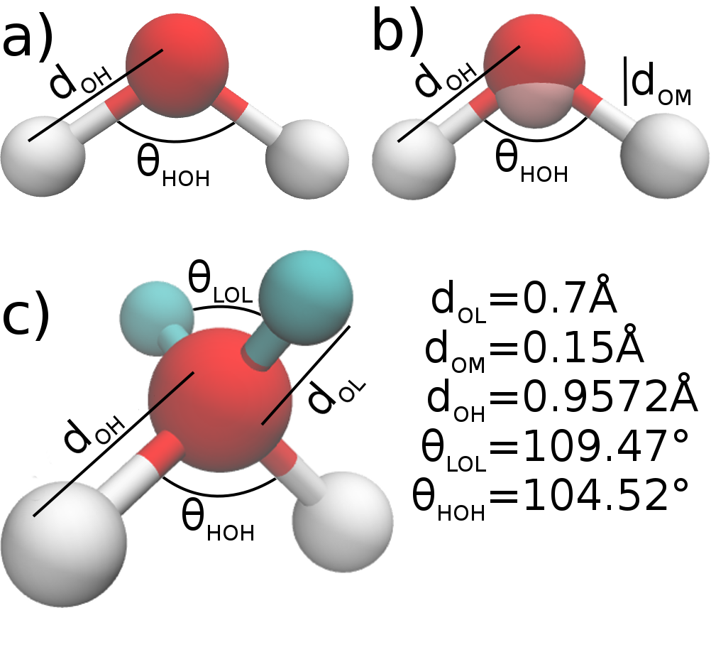
Figura 1: Geometries of TIP3P, TIP4P and TIP5P water models. a) Three point (3P) geometries only include positions of the oxygen and hydrogens. b) Four point (4P) geometries move the negative charge from the oxygen to a virtual site closer to the hydrogens. c) Five point (5P) geometries instead have two virtual sites to represent the oxygen’s Lewis pairs. In contrast to TIP5PMahoney and Jorgensen (2000a) and TIP5P-ERick (2004), TIP5P/2018 assigns charges to all the available five points.

II Methods

II.1 Initial Charge Assignment

Electrostatic potential (ESP) fittingMomany (1978); Cox and Williams (1981); Singh and Kollman (1984) is a classical approach to assigning charges for use in molecular dynamics (MD) potentials. It involves minimizing the difference between an ab initio reference electrostatic potential and that produced by the assigned charges on a grid within a region close the molecule. Grid points too close to the nuclei are excluded, as the electron density there has too much structure to be accurately represented by point charges. Similarly, grid points at large distances (typically $>$3\text{\,}\AA$$) are not taken into account for computational efficiency. The exact definition of the grid is method-specificBreneman and Wiberg (1990); Singh and Kollman (1984). One of known problems of these methods is that atoms embedded at the centers of larger molecules are assigned charges with values that are not chemically intuitive, mostly due to the lack of grid points nearby these atoms.

Restrained electrostatic potential (RESP) fittingBayly et al. (1993); Cornell et al. (1993) combats this by imposing a harmonic charge restraint of an a priori assigned weight preventing the assigned charges from significantly deviating from predetermined values, typically zeros. RESP has become popular for building force fieldsCieplak et al. (1995); Wang et al. (2004); Dupradeau et al. (2010), however in bulk water all the atoms effectively become embedded and have few surrounding grid points. Furthermore, these points are located in the empty space between the molecules. In molecular dynamics electrostatic forces act between pairs of nuclei, meaning that such a grid samples regions with low importance for parameterization. In this situation, the restraint of RESP plays a disproportionate role in charge assignment.

To avoid the above situation, we use a different approach. We determine the bulk wave function of a periodic 54 water molecule structure by Titantah and KarttunenTitantah and Karttunen (2015a) using CPMD 3.17.1CPM , the BLYP functionalBecke (1988); Lee et al. (1988) with D3 van der Waals correctionsGrimme et al. (2010); Hujo and Grimme (2013), pseudopotentials in Troullier-Martins form for oxygenTroullier and Martins (1991) and Kleinman-Bylander formKleinman and Bylander (1982) for hydrogen, and a $90\text{\,}\mathrm{R}\mathrm{y}$ plane wave energy cutoff. This wave function is then projected onto a Gaussian atom-centered basis. For this, we use the basis set for the Stuttgart/Dresden pseudopotentialsBergner et al. (1993), which are augmented, after uncontraction, by additional polarization functionsKrishnan et al. (1980) of $d$ symmetry. This results in a projection completeness above 99.95 %. We then subdivide the overall electron density into individual molecular contributions, which are determined from the full atomic-orbital density matrix after projection, by assigning its rows to the respective molecules. This ensures that electron density resulting from overlap of basis functions from two different molecules, described by off-diagonal blocks in the density matrix, is equally split among them.

The above subdivision allows one to compute molecular electrostatic potentials based on per-molecule electron densities that include the effects of polarization from other molecules in the bulk. At the same time, no grid points are excluded by the presence of other molecules in the setup of the grid for ESP fitting, permitting to sample the most relevant regions of the electrostatic potential for molecular dynamics. We implemented this procedure as a branch of the open source VOTCA-XTP packageXTP (2018) in a manner that includes Ewald summation for periodic systemsEwald (1921).

Next, we turn to the SQE formalismNistor et al. (2006); Nistor and Müser (2009) as a restraint-free alternative to RESP for charge assignment. SQE is a recent iteration on electronegativity and charge equilibration methodsMortier et al. (1985); Rappe and Goddard (1991); Rick et al. (1994). In contrast to earlier methods of this type, SQE combines both atom and bond based energy terms to enforce charge neutrality of interacting closed shell molecules without the need for charge restraints. It also introduces a penalty to long-range charge transfer, preventing long chain molecules from being overly polarizable, a problem common in the older techniquesLee Warren et al. (2008). SQE has been successfully used to describe redox reactions in batteriesDapp and Müser (2013a, b) and has been shown to reproduce the behavior of charges and electrostatic potentials in applied electric fieldsVerstraelen et al. (2012). Specifically, we rely on the SQE energy expression

$$U=\chi_{i}Q_{i}+\frac{1}{2}K_{i}Q_{i}^{2}+\frac{1}{2}\sum_{i}{\sum_{j}{K^{\mathrm{bond}}_{ij}(r_{ij})q_{ij}^{2}}}+U_{c}\,,$$ (2)

where $Q_{i}=\sum_{j}{q_{ij}}$ is the atomic charge assigned to atom $i$ as a result of contributions $q_{ij}=-q_{ji}$ from its covalently bonded neighbors $j$. The electronic parameters $\chi_{i}$ and $K_{i}$ represent electronegativity and atomic hardness, respectively. The distance-dependent bond hardness $K^{\mathrm{bond}}_{ij}(r_{ij})=\exp{(r_{ij}/\alpha_{ij})}-1$ acts as the penalty for charge transfer exceeding distances characterized by $\alpha_{ij}$. The energy due to Coulomb interactions $U_{c}$ between the charges includes the effects of periodicity, through Ewald summationEwald (1921), and intramolecular shielding (see Appendix).

For any set of the SQE parameters, atomic charges $Q_{i}$ can be obtained by minimizing Eq. 2 with respect to the charge transfers $q_{ij}$ along covalent bonds. We then apply the ESP procedure to iteratively optimize the SQE parameters and obtain a distribution of charges for each site. These distributions are very narrow with standard deviations of less than $0{,}014$ elementary charges. We use their means as the charges on a rigid five point (Fig. 1c) geometry in further potential refinement.

II.2 Parameter optimization

The charges obtained using the procedure above are combined with Lennard-Jones parameters fitted to reproduce the experimental dependence of density on temperature, especially the density peak at $4\text{\,}\mathrm{\SIUnitSymbolCelsius}$. At this stage, without further adjustments, the resulting potential yields significantly smaller diffusion than experiments ($1{,}60\times 10^{-5}$ compared to $2{,}30\text{\times}{10}^{-5}\text{\,}\mathrm{c}\mathrm{m}^{2}\mathrm{/}\mathrm{s}$ Pruppacher (1972)). In addition, the strength of the hard core repulsion required to correctly position the density peak is much larger than that of other water models. Besides the Lennard-Jones interaction, the only other interactions in the system are electrostatic, see Eq. 1. Therefore, to increase diffusion while maintaining the position of the density peak we explore scaling of the charges.

Uniform charge scaling has previously been suggested to correct ion binding strength for the CHARMM and AMBER forcefieldsLeontyev and Stuchebrukhov (2011). While integer ion charges represent the reality in vacuum, once inserted into water, the effective charge felt by the surrounding molecules is smaller due to screening. Non-polarizable water models can account for some of this effect explicitly by molecular rearrangement. However, without a polarizable description, screening due to changes in electron density are not explicitly accounted for. The electronic continuum correctionLeontyev and Stuchebrukhov (2010, 2011, 2012); Pluhařová et al. (2013); Vazdar et al. (2013); Kohagen et al. (2014); Kann and Skinner (2014); Kohagen et al. (2016) provides a way to implicitly model this effect by embedding the system in a continuous dielectric medium with a dielectric constant $\epsilon_{\mathrm{el}}$. This is equivalent to scaling the ionic charge $Q$ such that the effective charge is $Q_{\mathrm{eff}}=Q/\sqrt{\epsilon_{\mathrm{el}}}$. For liquid water the scaling factor is about 0.75Leontyev and Stuchebrukhov (2011) and the method has been successfully applied in simulations of biomolecular systemsMelcr et al. (2018); Duboué-Dijon et al. (2018).

The formulation of SQE we used in this work already includes the intramolecular electronic screening contributions through shielded electrostatic interactions (see Appendix). Intermolecular contributions, though, were not explicitly handled. Therefore, some charge scaling was still necessary. By scaling all charges by 0.95 and once again reoptimizing the Lennard-Jones parameters similar to Refs. Kohagen et al., 2014, 2016, we are able to recover the correct self-diffusion behavior. This is the parameterization of TIP5P/2018 as is detailed below in Sec. III.1.

All three TIP5P-based models have the same geometry, that is, an oxygen with the sole Lennard-Jones interaction site, two hydrogens $0{,}9572\text{\,}\AA$ from the oxygen and separated by a $104{,}52\text{\,}\mathrm{\SIUnitSymbolDegree}$ angle, and two virtual sites $0{,}7\text{\,}\AA$ from the oxygen separated by a perfect tetrahedral angle of $109{,}47\text{\,}\mathrm{\SIUnitSymbolDegree}$, Fig. 1c. The main difference between TIP5P/2018 and the previous TIP5P models is that charges are assigned to every site. The large portion of the charge that in the case of TIP5P is located on the virtual sites is instead on the oxygen. This reduces tetrahedrality (Sec. III.3), a problem TIP5P has been criticizedVega and Abascal (2011). The exact parameters of the TIP5P/2018 potential are presented in Table 1.

	TIP5PMahoney and Jorgensen (2000a)	TIP5P-ERick (2004)	TIP5P/2018
$Q_{O}$	0	0	-0.641114
$Q_{H}$	0.241	0.241	0.394137
$Q_{L}$	-0.241	-0.241	-0.073580
$\epsilon$ (kJ/mol)	0.66944	0.744752	0.79
$\sigma$ (Å)	3.12	3.097	3.145

Cuadro 1: Parameters defining five point models: site charges $Q$, Lennard-Jones potential well depth $\epsilon$, and distance of zero potential $\sigma$. All these five point potentials share the same geometry, Fig. 1c.

II.3 Computational details

The Gromacs 2016.3Abraham et al. (2015) software package was used for all MD simulations. All TIP5P/2018 simulations use a time step of $2\text{\,}\mathrm{fs}$, the smooth particle mesh Ewald methodEssmann et al. (1995) (SPME) for computing the electrostatic interactions and $0{,}85\text{\,}\mathrm{nm}$ cutoff for both the Lennard-Jones and real-space part of the Coulomb interactions. This cutoff is smaller than those of TIP5P and TIP5P-E, and has been adopted from TIP4P/2005 in an attempt to reduce the computational expense. Dispersion corrections for energy and pressure were also used. Unless stated otherwise, all thermostat and barostat time constants were set to $1\text{\,}\mathrm{ps}$ and all target pressures were set to $1\text{\,}\mathrm{a}\mathrm{t}\mathrm{m}$.

Thermodynamic properties across the range $235{,}65348{,}15\text{\,}\mathrm{K}$ were obtained by averaging over time and five $20\text{\,}\mathrm{ns}$ replicas at each temperature. Equilibration for each replica was performed as follows: First, a cubic simulation box with a side length of $4\text{\,}\mathrm{nm}$ containing 2,069 water molecules was set up and energy was minimized with the steepest descent algorithm. Next, a $10\text{\,}\mathrm{ps}$ simulation under the canonical ensemble with the Berendsen thermostatBerendsen et al. (1984) (with time constant $\tau_{t}=$0{,}5\text{\,}\mathrm{ps}$$) followed by a $20\text{\,}\mathrm{ps}$ isothermal-isobaric simulation with the Nosé-Hoover thermostatNosé (1984); Hoover (1985) ($\tau_{t}=$1\text{\,}\mathrm{ps}$$) and Berendsen barostatBerendsen et al. (1984) (at $1\text{\,}\mathrm{a}\mathrm{t}\mathrm{m}$ with time constant $\tau_{p}=$1\text{\,}\mathrm{ps}$$) was performed. After equilibration, $20\text{\,}\mathrm{ns}$ production simulation with Nosé-Hoover thermostatNosé (1984); Hoover (1985) ($\tau_{t}=$1\text{\,}\mathrm{ps}$$) and Parrinello-Rahman barostatParrinello and Rahman (1980, 1981) (at $1\text{\,}\mathrm{a}\mathrm{t}\mathrm{m}$, $\tau_{p}=$1\text{\,}\mathrm{ps}$$) followed. The first nanosecond of the production simulations was excluded from analysis as final equilibration.

Diffusion was computed from mean square displacement, while the thermodynamic properties were computed from drift corrected fluctuations of volume, density, and potential energy using standard formulasAllen and Tildesley (1987).

For comparison, we also performed control simulations with TIP4P/2005, TIP5P, and TIP5P-E. The TIP4P/2005 simulations were carried out under the same conditions as TIP5P/2018, except with $9\text{\,}\AA$ cutoffs. When simulating TIP5P and TIP5P-E, we used $9\text{\,}\AA$ cutoffs, 512 molecule systems, a $1\text{\,}\mathrm{f}\mathrm{s}$ time step, and no dispersion corrections, to match conditions under which they were parameterizedMahoney and Jorgensen (2000b); Rick (2004). To enforce densities originally reported for TIP5P and TIP5P-E, we used the canonical ensemble for both of these models. For TIP5P, we used the Berendsen thermostatBerendsen et al. (1984) with $\tau_{p}=$0{,}1\text{\,}\mathrm{ps}$$ and simple cutoffs, while for TIP5P-E we used the Nosé-Hoover thermostatNosé (1984); Hoover (1985) with $\tau_{p}=$1\text{\,}\mathrm{ps}$$ and SPME. Wherever possible, we compare properties of TIP5P/2018 to those of TIP5P and TIP5P-E reported by their original authors. Comparisons with experimental data are provided when possible.

III Results

The properties of TIP5P/2018 are summarized in Table 2 while their temperature dependencies are discussed in the sections below.

	$\rho$	$D$	$\alpha_{P}$	$\kappa$	$C_{P}$	$\epsilon$	$\tau_{1}^{\mathrm{dipole\,long}}$	$\tau_{2}^{\mathrm{HH\,long}}$
	($\mathrm{kg}\text{\,}{\mathrm{m}}^{-3}$)	($10^{-5}\times$${\mathrm{cm}}^{2}\text{\,}{\mathrm{s}}^{-1}$)	($10^{5}\times$${\mathrm{K}}^{-1}$)	($10^{6}\times$$\mathrm{a}\mathrm{t}\mathrm{m}^{-1}$)	($\mathrm{J}\text{\,}{\mathrm{mol}}^{-1}\text{\,}{\mathrm{K}}^{-1}$)		($\mathrm{ps}$)	($\mathrm{ps}$)
TIP5P	$999\pm 1$Mahoney and Jorgensen (2000a)	$2{,}62\pm 0{,}04$Mahoney and Jorgensen (2000b)	$63\pm 6$Mahoney and Jorgensen (2000a)	$41\pm 2$Mahoney and Jorgensen (2000a)	$122\pm 3$Mahoney and Jorgensen (2000a)	$82\pm 2$Rick (2004)	$5{,}788$	$2{,}506$
TIP5P-E	$1000{,}0\pm 0{,}5$Rick (2004)	$2{,}8\pm 1$Rick (2004)	$49\pm 6$Rick (2004)	$52\pm 3$Rick (2004)	$114\pm 3$Rick (2004)	$92\pm 14$Rick (2004)	$5{,}521$	$2{,}455$
TIP5P/2018	$996{,}30\pm 0{,}06$	$2{,}34\pm 0{,}02$	$42\pm 3$	$48{,}2\pm 0{,}5$	$105\pm 4$	$127\pm 4$	$6{,}575$	$2{,}901$
experimental	$997{,}05$Haynes (2015)	$2{,}30$Pruppacher (1972)	$25{,}7$Kell (1975)	$45{,}85$Kell (1975)	$75{,}36$Kell (1972)	$78{,}3$Malmberg and Maryott (1956)	$\approx 7{,}69$Rønne et al. (1997)	$\approx 2{,}46$Jonas et al. (1976)

Cuadro 2: Properties of TIP5P, TIP5P-E, and TIP5P/2018 at $298{,}15\text{\,}\mathrm{K}$ and $1\text{\,}\mathrm{a}\mathrm{t}\mathrm{m}$. Experimental densityHaynes (2015) is reported at $1\text{\,}\mathrm{b}\mathrm{a}\mathrm{r}$. The experimental values for $\tau_{1}^{\mathrm{dipole\,long}}$ and $\tau_{2}^{\mathrm{HH\,long}}$ are estimates linearly interpolated from measurementsRønne et al. (1997); Jonas et al. (1976) at nearby temperatures.

III.1 Density and Diffusion

Both the maximum density $\rho_{\mathrm{max}}$ and the corresponding temperature $T_{\mathrm{max}}$ for TIP5P/2018 match those of experimentsHaynes (2015); Hare and Sorensen (1987) (Fig. 2). This is a marked improvement over both TIP5P and TIP5P-E, which, while capturing the correct $T_{\mathrm{max}}$, exhibit an overly high $\rho_{\mathrm{max}}$ and a density that decays too rapidly. TIP5P/2018 significantly improves on the density decay compared to TIP5P and TIP5P-E, but is still unable to fully reproduce the experimental profile at high temperatures. Attempts to further flatten the density profile during potential optimization led to significantly lower diffusion accompanied by more first solvation shell structuring.

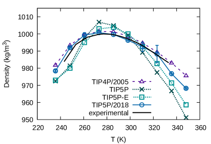
Figura 2: Density as a function of temperature at a pressure of $1\text{\,}\mathrm{a}\mathrm{t}\mathrm{m}$. TIP5P and TIP5P-E values are obtained from Ref. Rick, 2004. TIP5P/2018 and TIP4P/2005 values are results of our own simulations. Error bars for TIP5P/2018 represent standard deviations of the results from five simulations. Experimental dataHaynes (2015); Hare and Sorensen (1987) is shown for comparison

On the other hand, as Fig. 3 shows, TIP5P/2018 reproduces the diffusion profile extremely well, which is not surprising as it was one of the target properties during optimization. In comparison, TIP5P and TIP5P-E both exhibit much faster diffusion at higher temperatures while underestimating the experimental diffusion values at and below $262{,}65\text{\,}\mathrm{K}$. TIP4P/2005, meanwhile, underestimates diffusion at higher temperatures.

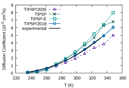
Figura 3: Self-diffusion as a function of temperature at a pressure of $1\text{\,}\mathrm{a}\mathrm{t}\mathrm{m}$. TIP5P and TIP5P-E values are obtained from Refs. Mahoney and Jorgensen, 2000a; Rick, 2004 and the experimental values from Refs. Holz et al., 2000; Price et al., 1999. TIP5P/2018 and TIP4P/2005 values are results of our own simulations. Error bars for TIP5P/2018 represent standard deviations of the results from five simulations.

III.2 Radial Distribution Functions

The radial distribution functions of TIP5P/2018 are in good agreement with experiments (Figs. 4, 5 and 6). The major discrepancy is the higher first peak of the oxygen-oxygen radial density function, Fig. 4. Additionally, neutron scattering experiments show a wide first peak for $g_{\mathrm{HH}}(r)$ (Fig. 6), which corresponds to the intramolecular H-H distance. Due to the rigidity of the five point potentials this distance is constrained to $1{,}5139\text{\,}\AA$ in the simulations, and appears as a sharp peak.

Rigidity of the five-point geometry also contributes to the first intermolecular $g_{\mathrm{OH}}(r)$ peak (Fig. 5), corresponding to the hydrogen bonding interaction. In all the five point models this peak is narrower and taller than in experiments. Rigid O-H covalent bonds in the simulations lead to reduced smearing of this peak from the optimal hydrogen bonding distance than is present in real water. Because of these effects, it is reasonable to assume that using a flexible geometry would better describe liquid water. However, a flexible model without explicit treatment of polarization tends to result in incorrect dipole moment dependence on geometry as discussed in Ref. Mahoney and Jorgensen, 2000a.

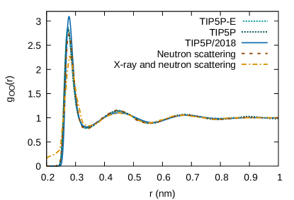
Figura 4: Oxygen-oxygen radial distribution functions for TIP5P/2018 ($298\text{\,}\mathrm{K}$), TIP5P ($298{,}15\text{\,}\mathrm{K}$), and TIP5P-E ($298{,}15\text{\,}\mathrm{K}$). Data for all these models comes from our own simulations. Experimental radial distribution functions from neutron scattering ($298\text{\,}\mathrm{K}$)Soper (2000) and combined X-ray and neutron scattering ($300\text{\,}\mathrm{K}$)Soper (2013) are also shown.

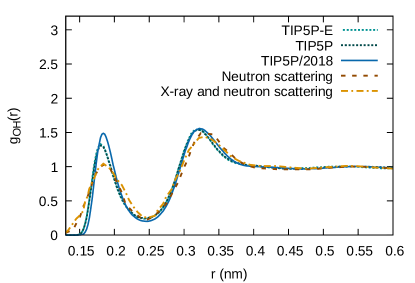
Figura 5: Oxygen-hydrogen radial distribution functions for TIP5P/2018 ($298\text{\,}\mathrm{K}$), TIP5P ($298{,}15\text{\,}\mathrm{K}$), and TIP5P-E ($298{,}15\text{\,}\mathrm{K}$). Data for all these models comes from our own simulations. Experimental radial distribution functions from neutron scattering ($298\text{\,}\mathrm{K}$)Soper (2000) and combined X-ray and neutron scattering ($300\text{\,}\mathrm{K}$)Soper (2013) are also shown.

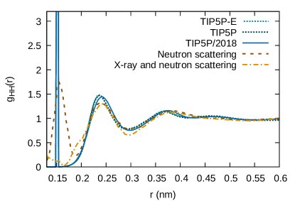
Figura 6: Hydrogen-hydrogen radial distribution functions for TIP5P/2018 ($298\text{\,}\mathrm{K}$), TIP5P ($298{,}15\text{\,}\mathrm{K}$), and TIP5P-E ($298{,}15\text{\,}\mathrm{K}$). Data for all these models comes from our own simulations. Experimental radial distribution functions from neutron scattering ($298\text{\,}\mathrm{K}$)Soper (2000) and combined X-ray and neutron scattering ($300\text{\,}\mathrm{K}$)Soper (2013) are also shown. The sharp peak near $1{,}5139\text{\,}\AA$ corresponds to the intramolecular hydrogen-hydrogen distance and is the result of using a rigid geometry.

III.3 Orientational Tetrahedral Order

The orientational tetrahedral order $q$ is a local measure of the angular alignment indicating how well the surroundings of a water molecule reproduce the regular tetrahedral structure (although slightly inconvenient here, we are using the notation of the original paper with $q$ denoting the tetrahedral order parameter). The expression we employ for $q$ was originally proposed by Chau and HardwickChau and Hardwick (1998) and rescaled by Errington and DebenedettiErrington and Debenedetti (2001) to produce values between 0 and 1,

$$q=1-\frac{3}{8}\sum_{j=1}^{3}\sum_{k=j+1}^{4}\left(\cos\phi_{jk}+\frac{1}{3}\right)^{2}\,,$$ (3)

where for any given water molecule indexes $j$ and $k$ iterate over the oxygens of its four nearest neighbors and $\phi_{jk}$ is the angle between these neighbors centered on the oxygen of the water molecule in question. A perfect tetrahedral arrangement, similar to that of hexagonal ice ($\text{I}_{\text{h}}$), occurs at $q=1$, while an ideal gas corresponds to $q=0$. Orientational tetrahedral order has previously been used to study both supercooled water and water in proximity to various solutes, as cited in Ref. Duboué-Dijon and Laage, 2015. For liquid water, distribution $f(q)$ typically exhibits two peaks corresponding to an ice-like population at high $q$ and a more disordered population at lower $q$. As temperatures grow, the more disordered population becomes preferred and the whole distribution shifts to lower values of $q$Overduin and Patey (2012); Titantah and Karttunen (2015b). TIP5P/2018 possesses the same behavior, however the high $q$ peak is shifted to the left compared to ab initio resultsTitantah and Karttunen (2015b), a feature shared with the TIP4P/2005 potentialOverduin and Patey (2012).

Additionally, TIP5P/2018 exhibits a larger disordered population than other models. The ratio of peak heights resembles that of other models at a higher temperature (Fig. 7). The simplest plausible explanation for this is too weak hydrogen bonding. This can be illustrated with the early version of our potential without charge scaling and, therefore, stronger hydrogen bonding. The corresponding $f(q)$ peaks of the earlier version are at the the same values of $q$, but with a larger preference for the ice-like peak, almost reaching that of TIP4P/2005Overduin and Patey (2012) and ab initio resultsTitantah and Karttunen (2015b). Unfortunately, the earlier versions of TIP5P/2018 exhibited drastically lower diffusion as a result of the increased hydrogen bonding and were deemed too inaccurate.

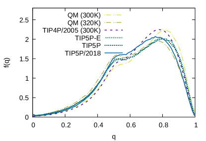
Figura 7: Normalized distributions of the orientational tetrahedral order $q$ for TIP5P/2018, TIP5P, and TIP5P-E at $298\text{\,}\mathrm{K}$, as well as TIP4P/2005 at $300\text{\,}\mathrm{K}$Overduin and Patey (2012) and ab initio distributions at $300\text{\,}\mathrm{K}$ and $320\text{\,}\mathrm{K}$Titantah and Karttunen (2015b). Data for all five point models is from our own simulations. TIP5P/2018 has angular structure akin to that of other potentials at higher temperature.

III.4 Dielectric Constant

The dielectric constant, also known as the relative permittivity $\epsilon$ of a material, is a key property for modeling the accurate solvation of ions. In molecular dynamics, $\epsilon$ is typically calculated from dipole moment fluctuations. Because of this, the value for the dielectric constant takes long simulation times to converge, especially at lower temperatures. The functional form proposed by NeumannNeumann (1983) is

$$\epsilon=1+\frac{1}{3\epsilon_{0}k{\langle T\rangle}{\langle V\rangle}}({\langle\vec{M}^{2}\rangle}-{\langle\vec{M}\rangle}^{2})\,,$$ (4)

where $\vec{M}$ is the total system dipole moment, $T$ is temperature, $V$ is the volume.

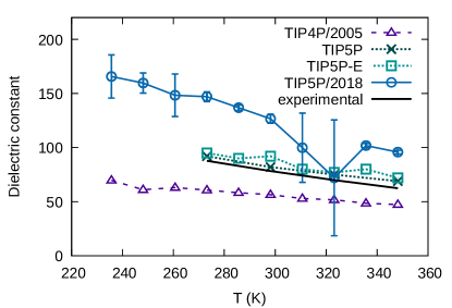
Figura 8: Dielectric constant of TIP5P/2018 as a function of temperature at a pressure of $1\text{\,}\mathrm{a}\mathrm{t}\mathrm{m}$ compared to those of other modelsMahoney and Jorgensen (2000a); Rick (2004) and experimental valuesMalmberg and Maryott (1956). Values for TIP4P/2005 and TIP5P/2018 are obtained from fluctuations of system dipole moment in our own simulations using standard formulasAllen and Tildesley (1987). Points and error bars for TIP5P/2018 represent standard deviations and means of the results from five simulations.

While TIP5P and TIP5P-E reproduce the experimentalMalmberg and Maryott (1956) temperature dependence of this property rather well, TIP5P/2018 significantly overestimates it (Fig. 8). As explored by Carnie and PateyCarnie and Patey (1982) and later by RickRick (2004), this overestimation can have two sources: a large molecular dipole moment $\mu$, and a small quadrupole. Both of the above works show that even at larger values of $\mu$, a large quadrupole can quench fluctuations of the system dipole moment and lower the dielectric constant.

	$\mu$	$Q_{xx}$	$Q_{yy}$	$Q_{zz}$
	(D)	(D Å)	(D Å)	(D Å)
TIP3PJorgensen et al. (1983)	2.35	-1.865	1.605	0.23
TIP4PJorgensen and Madura (1985)	2.18	-2.235	2.065	0.17
TIP4P/2005Abascal and Vega (2005)	2.305	-2.39	2.21	0.18
TIP5PMahoney and Jorgensen (2000a) and TIP5P-ERick (2004)	2.29	-1.63	1.50	0.13
TIP5P/2018	2.504	-1.91	1.69	0.21
QM surrounded by 4 TIP5PNiu et al. (2011)	2.69	-3.08	2.82	0.26
QM surrounded by 230 TIP5PCoutinho et al. (2003)	2.55	-2.91	2.71	0.20
Bulk QM (BLYP, $70\text{\,}\mathrm{R}\mathrm{y}$)Silvestrelli and Parrinello (1999)	2.95	-3.36	3.18	0.18
Bulk QM (BLYP, $60\text{\,}\mathrm{R}\mathrm{y}$)Site et al. (1999)	2.43	-2.77	2.67	0.10

Cuadro 3: Dipole $\mu$ and quadrupole $Q$ moments of TIP5P/2018 and similar non-polarizable potentials as well as some ab initio results for liquid water. Oxygen position is taken as the point of origin. The hydrogens are located in the positive $z$ half of the $yz$ plane, and the Lewis pairs in the $xz$ plane. Data presented for potentials other than TIP5P/2018 is derived from the work of Niu et al.Niu et al. (2011). The quadrupole moment definition of StoneStone (2013) is used.

Even after charge scaling, TIP5P/2018 has a relatively large dipole moment more in line with those obtained from ab initio simulations than with that of other rigid point charge potentials for water (Table 3). The quadrupole moment, on the other hand, is much smaller than in the ab initio systems, explaining the high dielectric constant. This is a consequence of assigning charges based on ESP fitting with a small number of charge sites. Reproducing both the dipole and the quadrupole moments becomes difficult in such casesNiu et al. (2011). This also illustrates why most water potentials are fully empirical by their nature.

A possible improvement could arise from using a six-point geometry, like that of Nada and van der EerdenNada and van der Eerden (2003), where the oxygen charge is shifted closer to the hydrogens, similar to what occurs in four point potentialsJorgensen and Madura (1985); Abascal and Vega (2005). Applying such a shift to existing charges would increase the quadrupole moment while decreasing the dipole moment. Furthermore, the central charge site would lie further away from the Lewis pairs, allowing them to capture more of the molecule’s ab initio charge distribution during ESP fitting and could potentially lend the resulting potential a larger quadrupole moment.

III.5 Thermodynamic Properties

The majority of the thermodynamic properties of TIP5P/2018 are in better qualitative agreement with experiments over a wider temperature range than the other five-point models are. The temperature dependence of the coefficient of thermal expansion $\alpha_{P}$ for TIP5P/2018 has the same shape as that of real water, but is slightly shifted toward higher values. While the corresponding profiles of both TIP5P and TIP5P-E cross the experimental profile near $280\text{\,}\mathrm{K}$, the TIP5P $\alpha_{P}$ changes significantly faster than in experiments and the TIP5P-E profile crosses the experimental line for a second time and returns back to positive values at low temperatures.

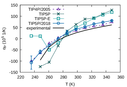
Figura 9: Coefficient of thermal expansion as a function of temperature at a pressure of $1\text{\,}\mathrm{a}\mathrm{t}\mathrm{m}$. TIP5P and TIP5P-E values are obtained from Refs. Mahoney and Jorgensen, 2000a; Rick, 2004, respectively, while experimental data is taken from Ref. Kell, 1975. Values for TIP4P/2005 and TIP5P/2018 are obtained from fluctuations of enthalpy, volume, and temperature in our own simulations. Error bars for TIP5P/2018 represent standard deviations of the results from five simulations.

The isothermal compressibility $\kappa_{T}$ of both TIP5P and TIP5P-E increases with temperature throughout the sampled range, while in experiments it decreases with temperature. TIP5P/2018 reproduces the experimental trend for temperatures down to $238{,}15\text{\,}\mathrm{K}$, albeit with a smaller slope (Fig. 10). Meanwhile, none of the five-point models are capable of reproducing the experimental isobaric heat capacity $C_{P}$ (Fig. 11), however TIP5P/2018 is the closest to experimental results. Overall, the improvements TIP5P/2018 provides for the reproduction of experimental $\alpha_{P}$ and $\kappa_{T}$ are remarkable given that they were not used as fitting targets and instead emerge naturally from the potential.

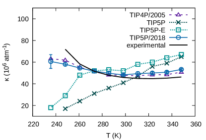
Figura 10: Isothermal compressibility as a function of temperature at a pressure of $1\text{\,}\mathrm{a}\mathrm{t}\mathrm{m}$. TIP5P and TIP5P-E values are obtained from Refs. Mahoney and Jorgensen, 2000a; Rick, 2004, respectively, while experimental data is taken from Ref. Kell, 1975. Values for TIP4P/2005 and TIP5P/2018 are obtained from fluctuations of volume and temperature in our own simulations. Error bars for TIP5P/2018 represent standard deviations of the results from five simulations.

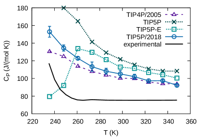
Figura 11: Isobaric heat capacity as a function of temperature at a pressure of $1\text{\,}\mathrm{a}\mathrm{t}\mathrm{m}$. TIP5P and TIP5P-E values are obtained from Refs. Mahoney and Jorgensen, 2000a; Rick, 2004, respectively, while experimental data is taken from Refs. Kell, 1972; Angell et al., 1973. Values for TIP4P/2005 and TIP5P/2018 are obtained from fluctuations of enthalpy and temperature in our own simulations. Error bars for TIP5P/2018 represent standard deviations of the results from five simulations.

III.6 Rotational degrees of freedom

While the radial distribution functions and the orientational tetrahedral order distribution provide a good description of structure, a different set of measures are required to analyze the dynamics. To characterize translational dynamics, we have already presented measurements of diffusion. For description of rotational dynamics of a rigid water geometry it is convenient to use rotational autocorrelation functions

$$\begin{split}C_{l}(t)={\big{\langle}P_{l}(\theta(t))\big{\rangle}}\,,\text{such that}\end{split}$$ (5)

$$\begin{split}\cos(\theta(t))=\frac{\vec{v}(t_{0}+t)\cdot\vec{v}(t_{0})}{\mathinner{\!\left\lVert\vec{v}\right\rVert}^{2}}\,,\end{split}$$ (6)

where $P_{l}$ are Legendre polynomials of order $l$, and $\vec{v}$ is a fixed magnitude vector the orientation of which is being studied. Experimentally, rotational autocorrelations have been measured for molecular dipole moments using dielectric spectroscopyBertolini et al. (1982); Rønne et al. (1997) ($l=1$), and the H-H vector using nuclear magnetic resonanceJonas et al. (1976); Lang and Lüdemann (1977) ($l=2$). In practice, these measurements are typically reported as rotational relaxation time constants, which we calculate by fitting double exponential curves to $0{,}25\text{\,}\mathrm{ns}$ long ($2{,}5\text{\,}\mathrm{ns}$ at temperatures below $250\text{\,}\mathrm{K}$) normalized rotational autocorrelation functions sampled every $0{,}5\text{\,}\mathrm{ps}$. For fitting, we use the double exponential form

$$a\exp\!\left[-\frac{t}{\tau_{l}^{\mathrm{type\,short}}}\right]+(1-a)\exp\!\left[-\frac{t}{\tau_{l}^{\mathrm{type\,long}}}\right],$$ (7)

where the superscript type corresponds to a molecular direction of either the dipole or the hydrogen-hydrogen vector (HH). With this formulation we can extract two time scales: one, $\tau_{l}^{\mathrm{type\,long}}$, corresponding to molecular reorientation due to changes in the hydrogen bonding network and the second, $\tau_{l}^{\mathrm{type\,short}}$, due to librations Jimenez et al. (1994); Luzar and Chandler (1996); Fecko et al. (2003).

The results show that TIP5P/2018 reproduces the experimental rotational relaxation of the molecular dipole moment better than TIP5P and TIP5P-E (Fig. 12) with values of $\tau_{1}^{\mathrm{dipole\,long}}=$6{,}58\text{\,}\mathrm{p}\mathrm{s}$$, $5{,}78\text{\,}\mathrm{p}\mathrm{s}$, and $5{,}52\text{\,}\mathrm{p}\mathrm{s}$ for the three potentials, respectively, at $298{,}15\text{\,}\mathrm{K}$, $1\text{\,}\mathrm{a}\mathrm{t}\mathrm{m}$. A linear interpolation of experimental dataRønne et al. (1997) produces a time scale of $7{,}69\text{\,}\mathrm{p}\mathrm{s}$ under the same conditions. Improvement in the rotational properties of the H-H vector are also present at lower temperatures (Fig. 13), but at higher temperatures TIP5P/2018 continues to slightly overestimate the experimental results with $\tau_{2}^{\mathrm{HH\,long}}=$2{,}90\text{\,}\mathrm{p}\mathrm{s}$$ at $298{,}15\text{\,}\mathrm{K}$, $1\text{\,}\mathrm{a}\mathrm{t}\mathrm{m}$, against the experimental value of approximately $2{,}46\text{\,}\mathrm{p}\mathrm{s}$, as interpolated from nearby temperature pointsJonas et al. (1976). The corresponding time scales for librations are $\tau_{2}^{\mathrm{HH\,short}}=$0{,}24\text{\,}\mathrm{p}\mathrm{s}$$ and $\tau_{1}^{\mathrm{dipole\,short}}=$0{,}50\text{\,}\mathrm{p}\mathrm{s}$$, however, due to the sampling time used, these values are less reliable. As TIP5P/2018 has a dipole moment magnitude close to those of QM descriptions of water (Table 3), the improvement of its rotational behavior is not surprising. Rotation of vectors perpendicular to the dipole moment, however, are also influenced by the quadrupole moment, which TIP5P/2018 underestimates, explaining the continued deviation from experiments for the H-H vector.

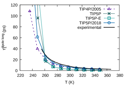
Figura 12: Temperature dependence of rotational decorrelation time $\tau_{1}^{\mathrm{dipole\,long}}$ of the dipole moment of TIP5P/2018 compared to other models and experimentsBertolini et al. (1982); Rønne et al. (1997). Values for all potentials are computed from our own simulations using double exponential fits (Eq. 7) to the autocorrelation functions.

Figura 13: Temperature dependence of rotational decorrelation time $\tau_{2}^{\mathrm{HH\,long}}$ of the molecular HH vector of TIP5P/2018 compared to other models and experimentsJonas et al. (1976); Lang and Lüdemann (1977). Values for all potentials are computed from our own simulations using double exponential fits (Eq. 7) to the autocorrelation functions.

III.7 TIP5P/2018 vs. TIP4P/2005: finite size effects

As TIP4P/2005 is currently the most accurate non-polarizable potential for water, it is useful to compare TIP5P/2018 against it. The two potentials provide very similar thermodynamic and rotational results. The main differences in the behaviors of the two are observable in the self-diffusion coefficients and the dielectric constants, both of which TIP4P/2005 underestimates. TIP5P/2018, on the other hand, overestimates the dielectric constant.

Furthermore, having been parameterized with a 360 molecule system, TIP4P/2005 has some drift in density as the system size increases (Fig. 14). Such finite size effects are a concern when parameterizing water potentials, as their typical use cases involve solvating biomolecules with a large amount of water to prevent the biomolecules from interacting with their own periodic images. To avoid such effects in TIP5P/2018, it was parameterized using 2069 molecules. This precaution may not have been needed, however, as for both TIP5P and TIP5P-E, having been parametrized for 512 molecule systems, our tests show little system size dependence. Overall, TIP5P/2018 offers improved reliability over TIP4P/2005, however this comes at an increase in computational expense of around 2.6 times.

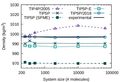
Figura 14: Density at $298{,}15\text{\,}\mathrm{K}$ and $1\text{\,}\mathrm{a}\mathrm{t}\mathrm{m}$ as a function of system size for TIP5P/2018 and common water potentials. Densities are based on $320\text{\,}\mathrm{ns}$ simulations with Nosé-Hoover thermostatNosé (1984); Hoover (1985) and Parrinello-Rahman barostatParrinello and Rahman (1980, 1981) with $1\text{\,}\mathrm{ps}$ time constants. Experimental densityHaynes (2015) is marked with a horizontal line. TIP5P and TIP5P-E systems are simulated with no dispersion corrections. TIP5P simulated with the smooth particle mesh Ewald (SPME) methodEssmann et al. (1995) is included for comparison here, as TIP5P combined with Ewald methodEwald (1921) variants is still a common sight todayShen et al. (2018); Yagasaki et al. (2018). The incorrect density produced by such combinations was one of the reasons for the creation of TIP5P-ERick (2004).

IV Summary and Outlook

We have shown the viability of using ab initio per-molecule electrostatic potentials as a basis for charge assignment for small molecules in dense periodic systems. We applied SQENistor and Müser (2009) as a more natural replacement for the charge constraint in the RESPBayly et al. (1993); Cornell et al. (1993) procedure. However, further refinement of this charge assignment approach is necessary, as not all electronic screening was taken into account. The resulting charges proved too large to accurately capture dynamical properties of water and uniform downscaling of the charge was required to reproduce the experimental self-diffusion coefficient with our final potential, TIP5P/2018.

Aside from correctly capturing the maximum density of liquid water by construction, TIP5P/2018 is also able to reproduce several emergent properties better than other five point potentials. Improvements include thermodynamic properties, especially the drastic improvement in the shape of the temperature dependence of isothermal compressibility, and rotational relaxation times. It offers comparable behavior to TIP4P/2005, but is more reliable in larger systems at the expense of an increased computational cost.

However, TIP5P/2018 still suffers in areas strongly dependent on its quadrupole moment, as it presents with a dielectric constant significantly higher than in experiments and possesses more preference for disordered angular configurations than other non-polarizable potentials and ab initio descriptions. Therefore, further improvements to our charge assignment procedure should focus on also reproducing the quadrupole moment of the reference ab initio charge distributions.

Apéndice A Coulomb interactions in SQE

Coulomb interactions $U_{c}$ in periodic systems typically rely on Ewald summationEwald (1921) to include long-range contributions, $U_{\mathrm{Ewald}}$. For charge assignment, however, we also include a shielding term $U_{\mathrm{shielding}}$ that applies the shielded electrostatic interaction ${J_{ij}(r_{ij})}$ only to intramolecular atom pairs.

$$U_{c}=U_{\mathrm{ewald}}+U_{\mathrm{shielding}}$$ (8)

$$U_{\mathrm{shielding}}=\frac{1}{2}\sum_{i}\sum_{j\neq i}Q_{i}Q_{j}({J_{ij}(r_{ij})}-1/r_{ij})$$ (9)

The $-1/r_{ij}$ term removes the nearest image interaction introduced by Ewald summation to be replaced by ${J_{ij}(r_{ij})}$, an approximation fitted to reproduce the shielded electrostatic interaction between two spherically symmetrical Slater-type orbitalsSlater (1960) via pairwise fitting parameters $k_{ij}$.

$${J_{ij}(r_{ij})}=\frac{1}{4\pi\epsilon_{0}}\frac{2/(1+e^{-k^{s}_{ij}r_{ij}})-1}{r_{ij}}$$ (10)

Atomic hardness $K_{i}$ of the SQE formalism can be recovered from the shielding interaction of an atom with itself, reducing the number of free parameters in the SQE potential.

$$K_{i}=\mathop{\operator@font l\acute{{\imath}}m}\limits_{r_{ii}\to 0}{J_{ii}(r_{ii})}$$ (11)

For larger molecules there is no need to apply ${J_{ij}(r_{ij})}$ to all pairs, as at larger distances it behaves as $1/r_{ij}$.