THE NANOGRAV 11-YEAR DATA SET: PULSE PROFILE VARIABILITY

Abstract

Access to 50 years of data has led to the discovery of pulsar emission and rotation variability on timescales of months and years. Most of this long-term variability has been seen in long-period pulsars, with relatively little focus on recycled millisecond pulsars. We have analyzed a 38-pulsar subset of the 45 millisecond pulsars in the NANOGrav 11-year data set, in order to review their pulse profile stability. The most variability, on any timescale, is seen in PSRs J1713$+$0747, B1937$+$21 and J2145$-$0750. The strongest evidence for long-timescale pulse profile changes is seen in PSRs B1937$+$21 and J1643$-$1224. We have focused our analyses on these four pulsars in an attempt to elucidate the causes of their profile variability. Effects of scintillation seem to be responsible for the profile modifications of PSR J2145$-$0750. We see evidence that imperfect polarization calibration contributes to the profile variability of PSRs J1713$+$0747 and B1937$+$21, along with radio frequency interference around 2 GHz, but find that propagation effects also have an influence. The changes seen in PSR J1643$-$1224 have been reported previously, yet elude explanation beyond their astrophysical nature. Regardless of cause, unmodeled pulse profile changes are detrimental to the accuracy of pulsar timing and must be incorporated into the timing models where possible.

1 Introduction

The radio emission from a pulsar can vary over a wide range of timescales. In practically all pulsars, the rotational phase, shape, and amplitude of individual radio pulses are known to vary considerably from one to the next with each rotation (e.g. Lyne et al., 1971; Taylor et al., 1975). The average shape of a few thousand pulses, however, is typically very stable and known as the pulse profile (e.g. Helfand et al., 1975; Rathnasree & Rankin, 1995). Soon after pulsars were discovered, however, changes in some pulse profiles were seen on short timescales in the form of mode-changing and nulling (Backer, 1970a, b). Mode-changing is a phenomenon in which pulsars switch between two or more quasi-stable emission states on timescales ranging from a few pulse periods to hours and days. In a nulling pulsar, one of these states shows little or no emission.

Pulsar data have now been collected for over 50 years. This allows us to also identify longer-term pulse profile variability. In 2006, the first known intermittent pulsar was identified by Kramer et al. (2006). Intermittent pulsars go through a quasi-periodic cycle between phases in which radio emission is, and is not, detected. The timescale of this behavior ranges from months to years (Camilo et al., 2012; Lorimer et al., 2012; Lyne et al., 2017). In intermittent pulsars, each state is associated with a different rate of rotational velocity loss, known as the spindown rate $\dot{\nu}$. Kramer et al. attribute $\dot{\nu}$ variations to global changes in magnetospheric particle currents; changing numbers of charged particles at the polar cap would simultaneously affect the pulsar’s radio emission. More links between pulse profile and rotation were provided in Lyne et al. (2010), an analysis that showed six pulsars for which $\dot{\nu}$ is correlated with changes in pulse shape over months and years. Further notable examples of long-term variability, including pulse profile and spindown correlation, continue to be found (e.g. Brook et al., 2014, 2016). All of the examples of long-term pulse profile variability given above are found in long-period pulsars (typically defined as those with spin periods above around 30 ms and those that have not been spun up or recycled through the accretion of matter from a companion star); relatively little work has been done regarding the long-term pulse profile variability of millisecond pulsars (MSPs). The issue of stability for MSPs is particularly important, however, as they are employed as high-precision timing tools that can facilitate fundamental studies of physics. For example, MSPs are used in pulsar timing arrays in an attempt to detect gravitational waves at nanohertz frequencies (Hobbs, 2013; Kramer & Champion, 2013; McLaughlin, 2013). MSPs are suitable for this role as they are known to be more rotationally stable than long-period pulsars due to their high angular momentum. Additionally, the time of arrival (TOA) of a pulse from an MSP can be measured with more precision than that of a long-period pulsar, as the uncertainty is proportional to the temporal width of a pulsar’s pulse profile.

A pulse TOA is measured by a process of template matching (Taylor, 1992; van Straten, 2006). The stability of a pulse profile at a given frequency permits the cross-correlation of an observed profile with a high signal-to-noise ratio (S/N) template, to provide a TOA of the former. The template is either the average of many previous observations, or a noise-free model of this average. Therefore, any unmodeled pulse profile changes will result in inaccurate pulse TOAs, which are detrimental to an MSP’s utility as a timing tool.

Pulse profile variability can be caused by any of the following: intrinsic changes in the pulsar and/or its magnetosphere, geodetic precession (Kramer, 1998; Hotan et al., 2005), torque-free precession (Stairs et al., 2000), propagation through the ionized interstellar medium (IISM), instrumental effects, and radio frequency interference (RFI). As well as the potential benefits for pulsar timing, understanding the causes of pulse profile variability and the sometimes correlated changes in rotational behavior may elucidate physical processes intrinsic to pulsars and their magnetosphere and also constrain the effects of pulse propagation.

As the long-term pulse profile variability of MSPs has not been well studied, it has only previously been reported in the MSP J1643$-$1224; Shannon et al. (2016) describe a sudden and permanent broadband pulse profile modification, accompanied by changes in timing.

In Brook et al. (2016), new techniques were used to identify pulse profile variability in long-period pulsar data collected by the Parkes Telescope. In this work we apply similar techniques to a large sample of MSPs using data recorded by the NANOGrav collaboration, with the aim of uncovering and quantifying MSP pulse profile variability. The NANOGrav collaboration produces TOAs by template matching the pulse profile in each frequency channel (typically between 5 and 64 over the observing band; Arzoumanian et al., 2015), thereby producing multiple TOAs for each observation. The analysis done here, however, looks for changes in pulse profiles that have been frequency-integrated over the observing band. This is done to maximize the S/N to facilitate the principal aim of characterizing the long-term profile behavior in the pulsar. However, when integrating a pulsar signal over a wide observing band, pulse profiles are more susceptible to variations induced by propagation effects (e.g. Pennucci et al., 2014).

In Section 2 we describe the NANOGrav data used for the variability analysis outlined in Section 3. The results of the analysis are presented in Section 4, followed by a discussion in Section 5. Conclusions are drawn in Section 6.

2 Data

The data analyzed in this paper are a subset of the NANOGrav 11-year data set (Arzoumanian et al., 2018), collected by the Green Bank Telescope (GBT) and Arecibo Observatory (AO). Since 2010, data collected by the GBT have been recorded by the Green Bank Ultimate Pulsar Processing Instrument (GUPPI; DuPlain et al., 2008; Ford et al., 2010). The observations are carried out at center frequencies around 820 and 1500 MHz. Since 2012, data collected at AO have been recorded by the Puerto Rican Ultimate Pulsar Processing Instrument (PUPPI). The observations are carried out at center frequencies around 327 MHz (PSR J2317$+$1439 only), 430 MHz, 1400 MHz and 2030 MHz. This GUPPI/PUPPI subset was used, as the instruments process a bandwidth of up to 800 MHz (divided into 1.5625 MHz frequency channels) depending on the mode of operation. Details of frequency coverage are given in Table 1 of Arzoumanian et al. (2015). Earlier narrow-bandwidth data in the NANOGrav data set were excluded from this analysis due to relatively low S/N.

GUPPI and PUPPI performed coherent dedispersion and folding in real-time. The data were folded at the dynamically calculated pulsar period using a pre-computed ephemeris to produce the pulse profile, consisting of 2048 phase bins. The pulsar signals were flux and polarization calibrated, and narrow-band RFI was removed in the manner of Arzoumanian et al. (2018).

The polarization calibration was done via an injected calibration signal that is generated by a local noise diode at 25 Hz. Preceding each pulsar observation, the noise diode signal is split, coupled into the two polarization paths and measured with the pulsar backends. This permits calibration of the differential gain and phase between the two hands of polarization. For a complete description of the instrumental response to a polarized signal, one must compute the Mueller matrix: a frequency-dependent linear transformation from the intrinsic to observed Stokes parameters (Heiles et al., 2001; van Straten, 2004). The Mueller matrix is determined by tracking a polarized source over a wide range of parallactic angles and fitting the resulting variation of the observed Stokes parameters as the feed rotates with respect to the sky. This allows the determination of effects such as the magnitude and phase of the cross coupling of the receiver arms.

While all the data sets have undergone noise diode calibration as described, full Mueller matrix calibration has also been performed on the 1500 MHz GUPPI data only. As this method provides more accurate pulse profile information, the GUPPI 1500 MHz profiles analyzed in this work have had full Mueller matrix calibration applied, unless stated otherwise. Mueller matrix calibration has also recently been applied to PUPPI data by Gentile et al. (2018), but their results have not been included in this analysis. The pulsed noise signals themselves were calibrated in on- and off-source observations of unpolarized continuum radio sources on a monthly basis.

Each final pulse profile analyzed here is the integration of typically 20 to 30 minutes of observation across the entire frequency band. Pulsars at declinations between 0 and +39 degrees were observed at AO while all others were observed with the GBT. PSRs J1713$+$0747 and B1937$+$21 were observed with both telescopes.

The dispersion measure (DM) is fit to the data at almost every observing epoch and applies for a window of up to 14 days, though typically much shorter. In NANOGrav timing analysis, an additional timing delay $\Delta t_{\rm{FD}}$ is added to all timing models to compensate for TOA perturbations induced by the frequency-dependence of pulse profile shapes. DM and $\Delta t_{\rm{FD}}$ are covariant when finding the best-fit timing model parameters for a pulsar, and so the best-fit DM value is highly dependent on $\Delta t_{\rm{FD}}$. For the purposes of creating the frequency-integrated pulse profiles employed in this variability analysis, we have calculated the best-fit DM parameters without the inclusion of $\Delta t_{\rm{FD}}$. This is discussed further in Section 5.4.

Further details of the observations, data reduction and timing models can be found in Arzoumanian et al. (2018) and references therein.

3 Analysis

The most effective metric for quantifying pulse profile variability is dependent on the timescales involved. Pulsar observations can often be widely and irregularly spaced; smooth trends that occur on timescales much longer than the time between these observations may not be obvious when analyzing individual pulse profiles. Such trends can instead be revealed when the variability is modeled and interpolated across many epochs of observation. If the pulse profile variations take place on timescales comparable to, or shorter than the span between observations, then any variability may appear stochastic, and a smooth trend (if one is present) may not be easily detected. The analysis techniques used to uncover and quantify both of these systematic and noisy types of pulse profile variability are described in the following.

To quantify the amount of pulse profile variability in an individual observation, we calculate the differences between the observed pulse profile and a constant model; these differences are termed the profile residuals (Brook et al., 2016). The model for a particular pulsar and observing frequency is a median profile; a median value is calculated in each individual phase bin using all observations in the pulsar data set. The median was used so that the model would be minimally affected by any outlying pulse profile shapes. The technique used to align the profiles before constructing the median model is simple cross-correlation. We note that the shape of the model is not crucial, as we are interested in how the observations change with time. The model merely defines the zero-point for the profile residuals.

Before the profile residuals can be calculated, the observations are processed to ensure that the off-pulse baseline is centered on zero. Any individual observations with highly irregular pulse profiles are treated as the result of RFI or instrumental issues and removed from further analysis. Additionally, the noisiest observations in a data set are considered unreliable and also excluded; an observation is removed if the standard deviation of the off-pulse region is more than a factor of two larger than the median value taken from the off-pulse regions across all epochs.

Pulse profile changes can manifest as a modulation of shape or as a change in flux density across the profile as a whole. Large flux density variations are observed in most of the pulsar data analyzed in this work, and are thought to be attributable to refractive and diffractive interstellar scintillation (RISS and DISS respectively; Rickett, 1990, e.g.). To disentangle the less common pulse profile shape changes, we must normalize the flux density of all observations. Alignment of the profiles with the constant model is also essential for the analysis that follows, as the timeseries in each pulse phase bin are modeled independently. This alignment is non-trivial; when profile deviations occur (either intrinsically or due to effects of propagation, instrumentation or RFI), it is possible that the alignment may be slightly biased in that direction when simple cross-correlation is employed. In this analysis, the flux density normalization and the phase alignment are carried out simultaneously in the following way.

3.1 Flux Density Normalization and Phase Alignment

In order to compare pulse profile shapes, we need to align them in phase and normalize them in flux density as effectively as possible. In many cases, the TOAs deviate enough from the pulsar timing model to disqualify their use in the alignment of the observations. Traditional profile alignment and normalization algorithms use $\chi^{2}$ minimization techniques and operate on all profile bins. These algorithms are susceptible to biases in cases when the two profiles differ in shape over some range of pulse phase. For this reason, we employed the following robust fitting algorithm, which is less susceptible to such biases. We characterize two pulse profiles as being correctly normalized and aligned by maximizing the number of phase bins that are in agreement; this is defined more formally below. Each observation, in turn, is normalized and aligned relative to the constant model. The observed profile is shifted in phase over the model. For each of the 2048 phase bin alignments, the scaling factor of the observation is varied over a range defined such that the observation’s profile peak is within 10% of the peak of the constant model. This range is sampled uniformly in 100 steps. The 10% restriction will reduce computation time while safely accommodating all realistic scaling trials. For each combination of phase shift and scaling factor, the absolute difference between model and observation is calculated in each phase bin along with the mean,

$$\delta=\frac{1}{n}\sum_{i}^{n}{|d_{i}-m_{i}|},$$ (1)

where $d_{i}$ and $m_{i}$ are the values of the observational data and the model (respectively) in phase bin $i$, and $n$ is the number of phase bins in the calculation. For identical profile shapes, for example, $\delta$ will be zero as the two profiles overlay exactly. We next exclude any phase bins in which $|d_{i}-m_{i}|$ is more than two standard deviations (2$\sigma$) away from $\delta$. After these outliers are removed, $\delta$ is then recalculated. This step is repeated until the recalculated mean $\delta$ changes by less than 0.1% of its previous value, at which stage the phase bin exclusion process is considered complete. The final number of phase bins that have not been excluded is $n_{\rm f}$. These steps are illustrated in Figure 1. All remaining bins now have relatively comparable values of $|d_{i}-m_{i}|$. This process is performed so that only the stable parts of the profile are used to align and scale, i.e. localized profile deviations that appear in observations are not required to match the constant model. To align and scale the profiles, we want to minimize the differences between the non-excluded phase bins, but also want to penalize fits in which only a small number of phase bins remain after the exclusion process. In order to find the optimal fit, we minimize $\delta$/$n_{\rm f}$.

In this analysis we calculate the variability of both normalized and non-normalized pulse profiles. The latter are also aligned using the technique above, but their flux density levels are restored at the end of the process.

Precision timing of pulsars demands that observations are aligned to fractions of a phase bin (under the assumption that the pulse profile is unchanging). However, aligning in single bin increments (with 2048 bin resolution) is simple, and sufficient in this profile profile variability analysis; any profile residuals produced by fractional phase bin misalignment would typically be insignificant when compared to the amount of noise in individual bins. If required, higher precision alignment could be implemented.

Once the pulse profiles are correctly aligned and normalized, we can proceed to calculate and analyze the profile residuals.

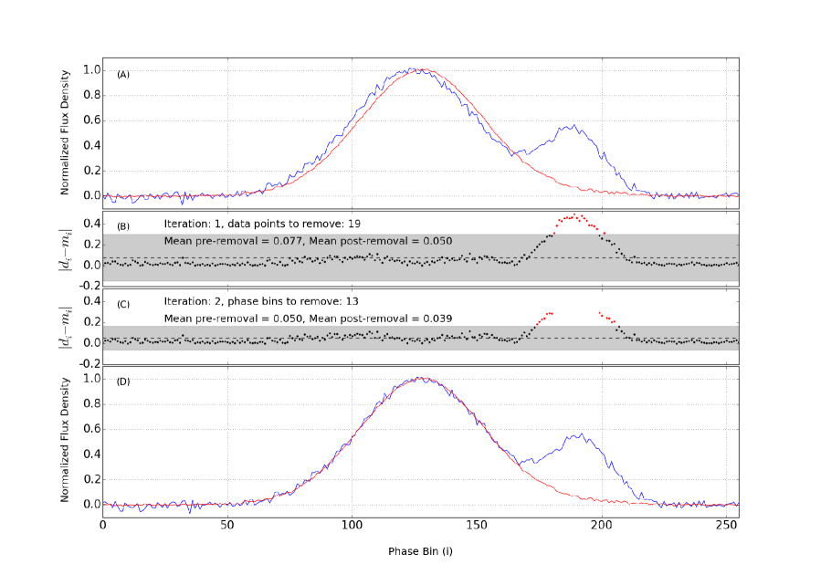
Figure 1: The method used to normalize and align pulse profiles. Panel A shows a simulated comparison of a model profile (red) and an observed profile (blue) with a trailing edge deviation. The alignment shown as an example, is the result of simple cross-correlation. For every alignment, a series of iterations, such as those illustrated in Panels B and C, are executed until a value for $\delta/n_{\rm f}$ is eventually determined (see text for details). In Panel B, the black dots show the absolute difference between the observed and model profiles in each phase bin ($|d_{i}-m_{i}|$). The dashed line indicates the mean and the gray band shows two standard deviations of the data; any points outside this band are removed before the standard deviation is recalculated and the process is repeated, as seen in Panel C. For each iteration, the mean of the data is calculated before and after the data removal. A change by less than 0.1% signifies the end of the process (14 iterations were required for this outlier removal in these simulated data shown in Panel A). The last data to be removed are restored and the final mean $\delta$ of $|d_{i}-m_{i}|$ is calculated. This value, divided by the number of contributing phase bins $\delta/n_{\rm f}$, is minimized whilst adjusting the phase and normalized flux density of the observation (relative to the model). Panel D is the relative alignment with the lowest value of $\delta/n_{\rm f}$.

3.2 Visualizing Variability

In Brook et al. (2016), a technique was developed that models pulse profiles as a function of time, allowing interpolation between the epochs of observation. For each of the pulse profile phase bins, we computed a Gaussian process (GP) regression model that best describes the profile residuals (Rasmussen & Williams, 2006; Roberts et al., 2012). The lengthscale hyperparameter for the GP regression models was constrained to between 30 and 300 days for every data set analyzed; we find that this requirement results in the data being well represented by the models. Full details of the GP regression analysis can be found in Brook et al. (2016). Examples of this inference technique are shown in Figure 2.

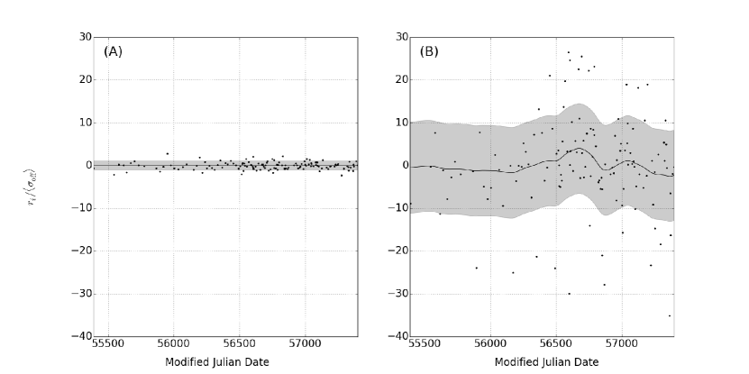
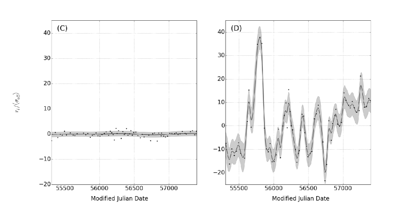
Figure 2: Profile residuals and their GP models. Panel A and Panel B show data from example off- and on-pulse phase bins respectively for PSR J1713$+$0747 at an observation frequency of 1500 MHz. Panel C and Panel D show data from example off- and on-pulse bins respectively for PSR B1937$+$21 at an observational frequency of 820 MHz. In each panel, the data points are the profile residuals for a single phase bin, the solid black line shows the GP mean and the gray area shows the GP standard deviation across the phase bin data set. Panel B is an example of a phase bin containing predominantly noisy data (with some systematic behaviour also embedded within), whereas the data in Panel D show a very clearly systematic trend, with relatively little noise. $r_{i}$ is the profile residual of bin $i$, $\langle\sigma_{\rm off}\rangle$ is the mean of the off-pulse profile residual standard deviation.

The individual phase bin models can be combined to produce a variability map for each pulsar. This is an interpolated plot that smoothly maps the evolution of a pulsar’s profile residuals with time. The GP regression technique can be used to identify subtle long-term trends that are not visible by eye, as demonstrated in Brook et al. (2016). For each pulsar discussed in Section 4, a variability map was produced for both pre- and post-normalization pulse profiles, so that the flux density of the observations can be compared with any profile shape changes seen.

The two pulsars in Figure 2 illustrate two different types of pulse profile variability (as mentioned at the beginning of Section 3). The systematic nature of the profile residuals in Panel D is well modeled by GP regression; the extent and nature of the profile variability is, therefore, easily captured by a variability map. In contrast, Panel B shows that the profile residuals in the J1713$+$0747 on-pulse phase bin are highly variable over time, but primarily in a noisy rather than systematic way. As a consequence, the GP model may infer little or no systematic variability and simply lie around the mean of the data points that inform it. The gray band in each Figure 2 panel shows the standard deviation of the model, however, and so provides an alternative measure of pulse profile variability. In order to show the amount of noisy variability for a pulsar data set, we also generate a color map showing the standard deviation of the GP model as a function of pulse phase and time. For instructional purposes, the color maps for a stable pulsar data set are shown in the Appendix (Figure 25).

3.3 Quantifying Variability

For each pulsar data set analyzed, we computed six metrics to fully describe the nature of the variability observed in the normalized pulse profiles. The metrics are defined as follows:

1. Ratio of (i) mean standard deviation of on-pulse phase bins to (ii) mean standard deviation of off-pulse phase bins: $\langle\sigma_{\rm on}\rangle/\langle\sigma_{\rm off}\rangle$.

   To calculate $\langle\sigma_{\rm on}\rangle$ we found the standard deviation of the profile residuals in each on-pulse phase bin and then calculated the mean across all epochs. The equivalent calculation was done for $\langle\sigma_{\rm off}\rangle$.

2. Ratio of (i) maximum standard deviation of on-pulse phase bins to (ii) mean standard deviation of off-pulse phase bins: $\sigma_{\rm on,max}/\langle\sigma_{\rm off}\rangle$.

   The maximum standard deviation of the profile residuals in individual on-pulse phase bins, provides information regarding any variability that may be concentrated over a small section of the pulse profile.

3. Ratio of (i) peak systematic variability to (ii) mean standard deviation of off-pulse phase bins: $\rm M_{\rm max}/\langle\sigma_{\rm off}\rangle$.

   $\rm M_{\rm max}$ is the peak value of the GP model over all on-pulse phase bins.

4. Ratio of (i) average systematic variability to (ii) mean standard deviation of off-pulse phase bins: $\langle\mid\rm M\mid\rangle/\langle\sigma_{\rm off}\rangle$.

   $\langle\mid\rm M\mid\rangle$ is the mean of the absolute value of the GP model for on-pulse phase bins.

5. Ratio of (i) noisy variability to (ii) mean standard deviation of off-pulse phase bins: $\langle\sigma_{\rm\rm M}\rangle/\langle\sigma_{\rm off}\rangle$.

   $\langle\sigma_{\rm\rm M}\rangle$ is the mean of the standard deviation of the GP model (i.e. the gray shaded regions in Figure  2) across all on-pulse phase bins. In pulsars with systematic variability (e.g. Panel D of Figure 2), the standard deviation about the GP model mean will be less than the standard deviation of the data themselves.

6. Ratio of (i) average systematic variability to (ii) noisy variability: $\langle\mid\rm M\mid\rangle/\langle\sigma_{\rm M}\rangle$.

   This metric is indicative of the amount of long-term, systematic variability in a data set.

An on-pulse phase bin is defined as one in which the flux density of the median profile for the data set is more than 3% of the peak. An off-pulse phase bin is defined as one in which the flux density of the median profile for the data set is less than 0.1% of the peak. The 3% and 0.1% values were chosen empirically to reliably select only on- and off-pulse phase bins respectively. The gap between the thresholds exists in order to avoid contamination between the two. If on- and off-pulse variability is comparable, metrics A and E will have a value around unity.

4 Results

The results of the pulse profile variability analysis are presented in Table 1, which is ordered by pulsar right ascension and then by observing frequency. Only the NANOGrav data sets that consist of 20 or more observations (after noisy and unreliable profiles are removed) are featured in the table. This is done to ensure that the GP regression has sufficient data points to infer an accurate model; 78 data sets (from a 38-pulsar subset of the 45 pulsars observed in the NANOGrav 11-year data set) remain after this requirement. The vast majority of pulsars show relatively little variability, with the mean standard deviation of their on-pulse phase bins being less than a factor of two greater than that of their off-pulse bins (Metric A of Table 1). The three pulsars for which this factor is greatest (denoted by an asterisk in Table 1) are PSRs J1713$+$0747, B1937$+$21 and J2145$-$0750. We have selected these pulsars for further analysis; below, we discuss the nature and possible causes of the profile variability for each of them. In addition, we also focus on PSR J1643$-$1224; after PSR B1937$+$21, the 820 MHz data set for this pulsar (denoted by a double asterisk in Table 1) has the largest average systematic to noisy variability ratio (Metric F of Table 1), which indicates the presence of long-term variability. PSR J1643$-$1224 has also previously demonstrated unusual chromatic timing behavior and long-term pulse profile shape changes (Shannon et al., 2016).

4.1 PSR J1713$+$0747

Due in part to the high S/N of its pulse profile, PSR J1713$+$0747 is one of the most precisely timed pulsars. Arzoumanian et al. (2018) list the standard deviation of the epoch-averaged timing residuals (the differences between observed TOAs and a timing model) for this pulsar as 116 ns over 11 years of NANOGrav observations. The high S/N also allows any pulse profile variations to be seen clearly.

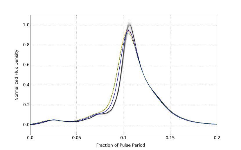
Figure 4: The pulse profile variability seen in PSR J1713$+$0747 at 1400 MHz. The orange, blue and green (dashed) profiles were observed on MJDs 56360, 56598 and 57239 respectively. The gray profiles show the other 58 pulse profiles in the data set. See also Figure 18 and Section 5.4 for a comparision of these three noteworthy observations to profile changes caused by inaccurate DMs in this data set.

The 1400 MHz AO observations of PSR J1713$+$0747 display the most profile variability of all data sets analyzed in this work; Table 1 shows that this is mostly noisy in nature (a relatively large value for variability metric E and a relatively small value for variability metric F). Despite the average systematic variability of the data set being low with respect to the noisy variability, the peak of the systematic variability is high; the GP model is being strongly affected over short time periods by three observations with anomalous profile shapes (MJDs 56360, 56598 and 57239). This can be seen in the variability map in Panel B3 of Figure 3. These three profiles are compared to those typical for the data set in Figure 4. For the observation made on MJD 56360, it is known that during the flux density calibration procedure, an incorrect pulsed calibration signal was injected at the epoch of observation. It is not clear whether the pulse profile shape was affected by this. However, no such calibration issues exist for the observations made on MJDs 56598 or 57239. In the “Discussion” section, we compare these three profiles to those expected to be produced by inaccurate DM measurements. This is shown in Figure 4 and described in Section 5.4.

Table 1: The variability calculated in 78 NANOGrav MSP data sets.

Pulsar	Observing	$\langle\sigma_{\rm on}\rangle/\langle\sigma_{\rm off}\rangle$	$\sigma_{\rm on,max}/\langle\sigma_{\rm off}\rangle$	$\rm M_{\rm max}/\langle\sigma_{\rm off}\rangle$	$\langle\mid\rm M\mid\rangle/\langle\sigma_{\rm off}\rangle$	$\langle\sigma_{\rm\rm M}\rangle/\langle\sigma_{\rm off}\rangle$	$\langle\mid\rm M\mid\rangle/\langle\sigma_{\rm M}\rangle$
Name	Frequency
	(MHz)	(A)	(B)	(C)	(D)	(E)	(F)
J0023$+$0923	430	1.13	1.97	3.58	0.12	1.10	0.11
J0023$+$0923	1400	1.17	2.74	3.69	0.08	1.17	0.07
J0030$+$0451	430	1.02	1.76	2.81	0.06	1.02	0.06
J0030$+$0451	1400	1.03	1.72	1.97	0.05	1.03	0.05
J0340$+$4130	820	1.03	1.70	1.95	0.08	1.02	0.08
J0340$+$4130	1500	1.00   1.00	1.42   1.38	3.07   3.44	0.09   0.09	0.98   0.99	0.09   0.09
J0613$-$0200	820	1.08	3.01	3.56	0.11	1.06	0.10
J0613$-$0200	1500	1.04   1.04	1.47   1.70	3.92   3.16	0.08   0.08	1.03   1.03	0.08   0.08
J0636$+$5128	820	1.10	1.63 4.16	0.14	1.07	0.13
J0636$+$5128	1500	1.08   1.07	1.74   1.64	4.34   3.54	0.10   0.13	1.06   1.02	0.10   0.13
J0645$+$5158	820	1.06	2.30	3.47	0.09	1.04	0.09
J0645$+$5158	1500	1.06   1.05	2.09   2.12	5.96   5.72	0.10   0.12	1.03   1.02	0.10   0.12
J0931$-$1902	820	1.03	1.71	4.14	0.11	1.01	0.11
J0931$-$1902	1500	1.09   1.05	2.08   1.87	3.73   3.79	0.11   0.12	1.08   1.02	0.10   0.12
J1012$+$5307	820	1.09	1.77	3.57	0.12	1.07	0.11
J1012$+$5307	1500	1.13   1.12	2.92   2.64	3.39   2.56	0.06   0.09	1.12   1.11	0.05   0.08
J1024$-$0719	820	1.06	1.72	3.59	0.09	1.04	0.09
J1024$-$0719	1500	1.05   1.06	1.71   1.80	3.56   3.31	0.10   0.08	1.03   1.05	0.10   0.08
J1125$+$7819	820	1.04	1.71	4.21	0.15	0.99	0.15
J1455$-$3330	820	1.10	2.04	3.44	0.11	1.09	0.10
J1455$-$3330	1500	1.09   1.07	3.00   2.71	5.75   6.23	0.16   0.15	1.04   1.02	0.15   0.15
J1600$-$3053	820	1.05	1.40	2.36	0.09	1.04	0.09
J1600$-$3053	1500	1.15   1.24	2.10   2.96	1.99   6.31	0.08   0.10	1.14   1.23	0.07   0.08
J1614$-$2230	820	1.02	1.39	2.99	0.09	1.00	0.09
J1614$-$2230	1500	1.01   1.00	1.29   1.33	2.59   1.91	0.05   0.06	1.00   1.00	0.05   0.06
J1640$+$2224	430	1.07	1.63	2.57	0.04	1.07	0.04
J1640$+$2224	1400	1.32	2.85	2.75	0.08	1.32	0.06
**J1643$-$1224	820	1.14	1.75	3.40	0.29	1.05	0.28
J1643$-$1224	1500	1.01   1.00	1.42   1.32	2.33   2.26	0.09   0.09	1.00   0.99	0.09   0.09
J1713$+$0747	820	1.36	5.11	3.33	0.12	1.35	0.09
*J1713$+$0747	1400	8.78	52.19	269.88	0.89	8.65	0.10
J1713$+$0747	1500	2.38   2.21	12.47   11.54	6.85   6.23	0.12   0.27	2.36   2.18	0.05   0.12
J1713$+$0747	2030	3.36	11.58	4.08	0.10	3.39	0.03
J1738$+$0333	1400	1.34	6.00	5.88	0.14	1.29	0.11
J1741$+$1351	430	1.22	3.09	3.70	0.16	1.17	0.14
J1741$+$1351	1400	1.11	2.37	3.52	0.10	1.10	0.09
J1744$-$1134	820	1.12	1.56	3.00	0.11	1.10	0.10
J1744$-$1134	1500	1.38   1.35	2.26   2.45	2.41   3.71	0.11   0.11	1.37   1.34	0.08   0.08
J1747$-$4036	820	1.03	1.68	2.44	0.12	1.01	0.12
J1747$-$4036	1500	1.03   1.03	1.52   1.62	3.05   2.97	0.12   0.11	1.01   1.01	0.12   0.11
J1832$-$0836	820	1.02	1.55	2.69	0.09	1.01	0.09
J1832$-$0836	1500	1.03   1.03	1.49   1.66	3.04   4.91	0.09   0.10	1.01   1.00	0.09   0.10
J1853$+$1303	430	1.06	1.82	2.85	0.08	1.06	0.08
J1853$+$1303	1400	1.07	1.66	4.46	0.10	1.05	0.10
B1855$+$09	430	1.03	1.46	3.61	0.08	1.02	0.08
B1855$+$09	1400	1.25	3.77	3.98	0.11	1.24	0.09
J1903$+$0327	1400	1.10	1.75	3.19	0.21	1.05	0.20
J1903$+$0327	2030	1.10	2.00	4.90	0.13	1.08	0.12
J1909$-$3744	820	1.59	2.95	3.65	0.24	1.54	0.16
J1909$-$3744	1500	1.65   1.58	3.12   2.81	1.51   1.74	0.04   0.07	1.65   1.58	0.02   0.04
J1910$+$1256	1400	1.03	1.59	2.89	0.08	1.02	0.08
J1910$+$1256	2030	1.04	1.58	4.76	0.17	0.99	0.17
J1918$-$0642	820	1.03	1.42	1.96	0.08	1.02	0.08
J1918$-$0642	1500	1.05   1.05	1.58   1.54	1.92   3.04	0.05   0.06	1.05   1.04	0.05   0.06
J1923$+$2515	430	1.06	2.00	2.93	0.09	1.05	0.09
J1923$+$2515	1400	1.09	1.95	5.11	0.10	1.07	0.09
*B1937$+$21	820	5.35	12.20	37.01	2.69	3.60	0.75
B1937$+$21	1400	5.09	12.86	23.42	0.91	4.82	0.19
B1937$+$21	1500	5.07   3.36	10.85   7.76	3.82   3.24	0.42   0.39	5.05   3.33	0.08   0.12
B1937$+$21	2030	2.93	8.30	14.32	1.31	2.36	0.56
J1944$+$0907	430	1.09	1.96	3.38	0.10	1.08	0.09
J1944$+$0907	1400	1.12	2.06	3.91	0.13	1.09	0.12
B1953$+$29	430	1.10	1.91	4.22	0.22	1.03	0.21
B1953$+$29	1400	1.03	1.52	4.25	0.09	1.01	0.09
J2010$-$1323	820	1.14	2.76	3.59	0.09	1.12	0.08
J2010$-$1323	1500	1.10   1.10	2.33   2.42	2.80   2.37	0.06   0.07	1.09   1.10	0.06   0.06
J2017$+$0603	1400	1.11	5.55	5.47	0.15	1.08	0.14
J2017$+$0603	2030	1.16	3.46	7.79	0.17	1.13	0.15
J2043$+$1711	430	1.05	1.62	2.39	0.03	1.05	0.03
J2043$+$1711	1400	1.04	1.74	5.11	0.10	1.02	0.10
*J2145$-$0750	820	1.76	8.62	3.79	0.31	1.72	0.18
J2145$-$0750	1500	1.37   1.31	3.02   3.51	4.69   3.82	0.22   0.15	1.32   1.28	0.17   0.12
J2214$+$3000	1400	1.00	1.73	5.37	0.12	0.97	0.12
J2302$+$4442	820	1.02	1.57	2.34	0.07	1.01	0.07
J2302$+$4442	1500	1.04   1.00	1.54   1.56	4.73   2.66	0.10   0.09	1.01   0.99	0.10   0.09
J2317$+$1439	327	1.13	2.15	3.07	0.13	1.10	0.12
J2317$+$1439	430	1.10	1.80	2.52	0.04	1.10	0.04
J2317$+$1439	1400	1.07	1.78	2.81	0.07	1.06	0.07

Note. — An asterisk denotes each of the three data sets with the highest values for the ratio of the mean standard deviation of on- to off-pulse phase bins (Metric A; a measurement of the level of profile variability of any kind). These data are from the PSRs J1713$+$0747, B1937$+$21 and J2145$-$0750. Highlighted with a double asterisk is the 820 MHz data set for PSR J1643$-$1224, which has the highest ratio of average systematic to noisy variability (Metric F; a measurement of the significance of systematic variability) after PSR B1937$+$21. Each of the six variability metrics is described in Section 3.3. The data sets observed with the GBT at 1500 MHz have two values for each variability metric. The left of the pair relates to profiles calibrated by the noise diode, and the right to profiles that additionally have full Mueller matrix calibration applied (see Section 2).

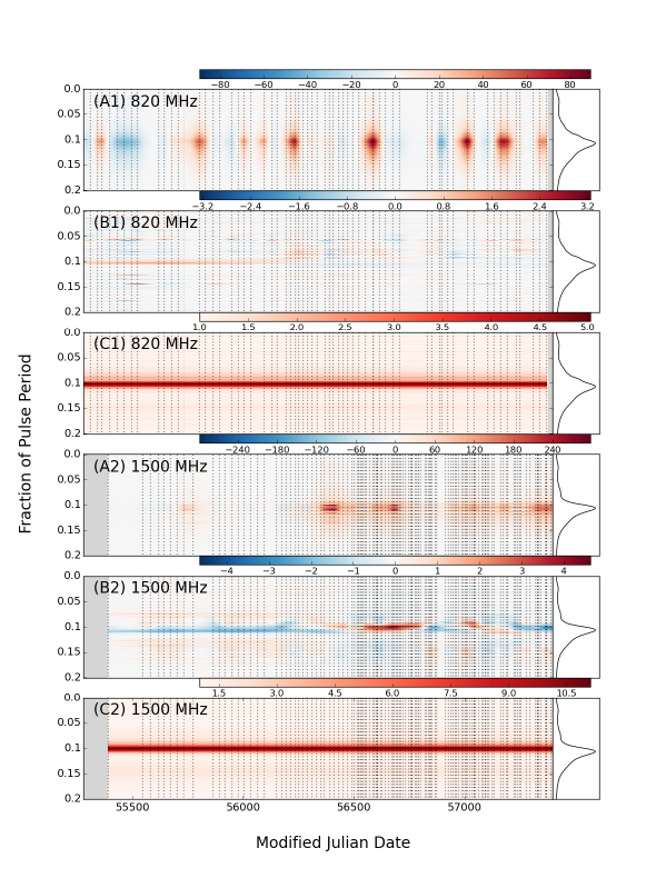
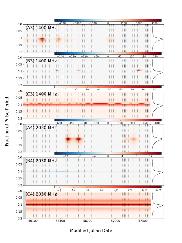
Figure 3: Variability maps for PSR J1713$+$0747, for central observing frequencies of 820 MHz (GBT), 1500 MHz (GBT), 1400 MHz (AO) and 2030 MHz (AO). Panel labels prefixed with an A are variability maps showing the flux density variations in the flux-calibrated, pre-normalized observations. Those prefixed with a B show pulse profile shape changes after the observations have been normalized. In all of these variability maps, red regions indicate where the inferred pulse profile has an excess of flux density (normalized or otherwise) compared to the average for the data set. Blue indicates where it has a deficit. Panel labels prefixed with a C map the standard deviation of the GP model as a function of pulse phase and time. The vertical dotted lines indicate the epochs of observation informing the GP models. The unit for all panels is the mean of the standard deviation of the off-pulse phase bins for the relevant data set. Panel sections for which there is no data, are gray. To the right of each panel, the average pulse profile for the data set is shown.

The observations made at 2030 MHz show a high degree of noisy variability, particularly in the latter half of the data set; the ratio of average systematic to noisy variability $\langle\mid\rm M\mid\rangle/\langle\sigma_{\rm M}\rangle$ is the smallest of all data sets. The ratio of the mean standard deviation of the on- to off-pulse phase bins $\langle\sigma_{\rm on}\rangle/\langle\sigma_{\rm off}\rangle$ is not as large as that of the 1400 MHz data set, however, because at 2030 MHz, $\langle\sigma_{\rm off}\rangle$ is much larger.

All PSR J1713$+$0747 data sets are dominated by noisy variability, i.e. profile shape changes largely occur on timescales shorter than the time between observations, and so the noisy variability far exceeds any systematic variability modeled by the GP. Some systematic variability is present, however; the PSR J1713$+$0747 data set with the highest ratio of average systematic to noisy variability (Metric F of Table 1) is recorded at 1500 MHz. Panel B of Figure 2 depicts the systematic behavior of the GP model (embedded in the primarily noisy variability) in an individual phase bin for the data set. The bin is associated with a pulse period fraction of $\sim$ 0.1 in Panel B2 of Figure 3.

As the variability in the PSR J1713$+$0747 data sets is predominantly short-term in nature, it is difficult to compare even the pulse profiles that were observed at similar frequencies, unless they are also observed at the same time. The 1400 MHz AO and 1500 MHz GBT observations are often made just days apart, but only simultaneous observations could permit us to observe identical pulse profile shapes and allow us to confirm the nature of any profile variability seen, as astrophysical.

4.2 PSR B1937$+$21

PSR B1937$+$21 was the first MSP discovered (Backer et al., 1982) and with a rotational frequency of 642 Hz, remained the most rapidly spinning pulsar known for 24 years after it was found. This bright, isolated MSP is one of the most precisely timed pulsars, with the root mean square (rms) value of the white noise component for the 11-year data set residuals being 109 ns (Arzoumanian et al., 2018). It is also, however, one of the few MSPs that displays measurable timing noise (Shannon & Cordes, 2010). Including both the red and white noise components of the timing residuals, the rms calculated by Arzoumanian et al. jumps up to 1.5 $\mu$s. Suggested interpretations of the red noise include intrinsic changes in the spindown rate of the pulsar (Kaspi et al., 1994), interstellar propagation effects (Armstrong, 1984; Rickett, 1990; Kaspi et al., 1994; Cognard et al., 1995) and the presence of a circumpulsar asteroid belt (Shannon et al., 2013). PSR B1937$+$21 has also been seen to exhibit giant pulses; around one in every 10,000 individual pulses has more than 20 times the mean on-pulse flux density and some pulses have around 300 times this average (Cognard et al., 1996). This behavior is seen in both the main and interpulse components, which are separated by approximately half a pulse period. In our pulse profile analysis, PSR B1937$+$21 shows the most systematic variability, present primarily at 820 and 2030 MHz and in both the main and interpulse components. This can be seen in Metric F of Table 1, where the ratios of systematic to noisy variability for PSR B1937$+$21 are much higher than those for PSR J1713$+$0747. Panels B1 and B4 of Figures 5 and 6 also clearly highlight the systematic evolution of the pulse profile shape over time. The variability inferred by the GP model at 2030 MHz between $\sim$ MJDs 57000 and 57300 (see Panel B4 of Figures 5 and 6) is induced by three consecutive pulse profiles. They are compared with the rest of the profiles in the data set in Figure 7. See also the discussion around polarization calibration in Section 5.6 and Figure 23.

A direct comparison between the profile variability seen by AO at 1400 MHz and by GBT at 1500 MHz is made difficult primarily because the observations at this frequency have the smallest ratio of systematic to noisy variability of the PSR B1937$+$21 data sets (Metric F of Table 1). Therefore, much of the variability is noisy, but only longer timescale systematic trends can be directly compared, as the observations are generally not made on the same days. Some systematic structure appears in the 1500 MHz GBT observation (Panel B2 of Figures 5 and 6), but the units of these panels show that the systematic variability is weak, with the GP model reaching levels only a few times higher than the levels of off-pulse noise. At such levels, the GP model can be substantially influenced by the behavior of even one or two pulse profiles. Additionally, the GBT and AO data sets analyzed here span different dates; much of the systematic variability in the 1500 MHz GBT observations occurs around MJD 56000, which is before the 1400 MHz AO data were recorded by PUPPI. Furthermore, the relatively sparse sampling of the AO observations also inhibits direct comparison with the GBT GP variability models.

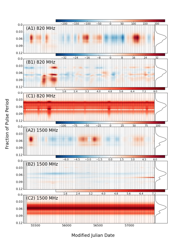
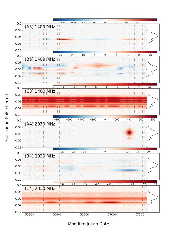
Figure 5: Variability maps for the main pulse of PSR B1937$+$21. Otherwise as Figure 3.

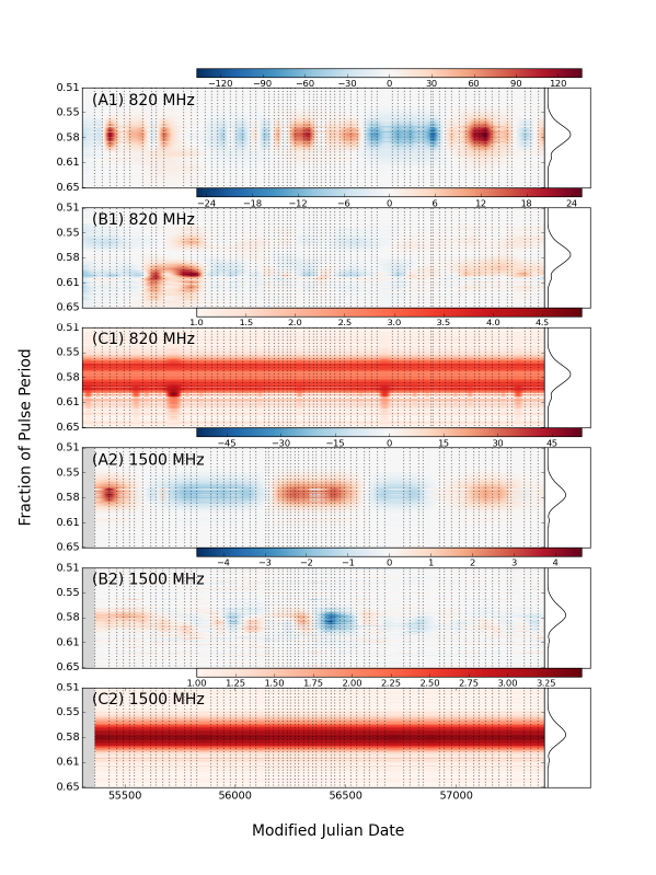
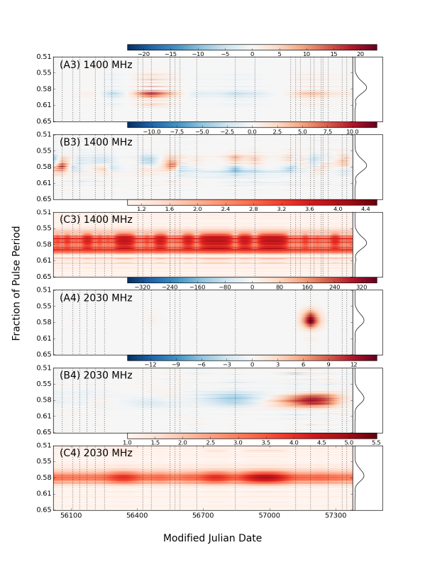
Figure 6: Variability maps for the interpulse of PSR B1937$+$21. Otherwise as Figure 3.

Figure 7: The pulse profile variability of PSR B1937$+$21 at 2030 MHz. The main panel shows the main pulse, and the inset is the interpulse. The orange, blue and green profiles were observed on MJDs 57117, 57185 and 57265 respectively. The gray profiles show the other 17 pulse profiles in the data set. See also the discussion around polarization calibration in Section 5.6 and Figure 23.

4.3 PSR J2145$-$0750

PSR J2145$-$0750 has the third highest variability levels (by the metric in Metric A of Table 1) of the pulsars in our analysis. It is found to have a mean standard deviation of on-pulse phase bins that is a factor of 1.76 larger than that of the off-pulse phase bins (at 820 MHz). As with PSR J1713$+$0747, most of the variability is noisy; Panel B1 of Figure 8 shows a long-timescale change in the pulse profile shape, but the magnitude of this change is small compared to the standard deviation of the data (Panel C1).

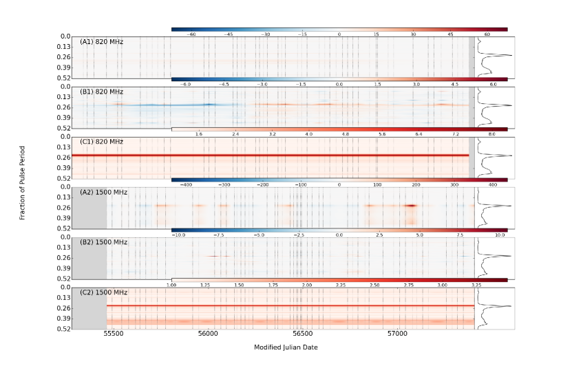
Figure 8: Variability maps for PSR J2145$-$0750. Otherwise as Figure 3.

4.4 PSR J1643$-$1224

PSR J1643$-$1224 has been observed since 2003 as part of the Parkes Pulsar Timing Array project (Manchester et al., 2013) at 700, 1400 and 3100 MHz. Shannon et al. (2016) noticed TOA perturbations, which they attributed to unmodeled changes in pulse shape, observed to occur around MJD 57074 (2015 February 21). These timing perturbations are most significant at 3100 MHz, and Shannon et al. only show profile changes at that frequency. Figure 9 provides a comparison of the pulse profile shapes of PSR J1643$-$1224 before and after 2015 February 21, as observed by the GBT. The upper panels show a significant difference at 820 MHz, but little change at 1500 MHz. Shannon et al. (2016) compare the shape variations of PSR J1643$-$1224 to those observed in PSR J0738$-$4042 (Karastergiou et al., 2011) and also point out that the new components are unpolarized in both pulsars. A new component is seen to appear in PSR J0738$-$4042 after a drifting feature is observed to move centrally over a span of $\sim$ 100 days (Brook et al., 2014). The variability map in Panel B1 of Figure 10 shows that changes in the profile shape appear to be occurring across the data set, and not just abruptly after MJD 57074. In particular, red colored drifting features can be seen at the beginning and end of the data set. The drifting at the end of the data, in which an emission feature moves away from the center of the pulse profile over a few hundred days, is more clearly shown in Figure 12.

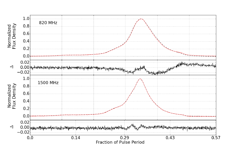
Figure 9: The combined pulse profiles of PSR J1643$-$1224 before (red) and after (black dashed) MJD 57074 (2015 February 21). The narrower panels show the red profile minus the black dotted profile ($\Delta$). All profiles are normalized to the peak.

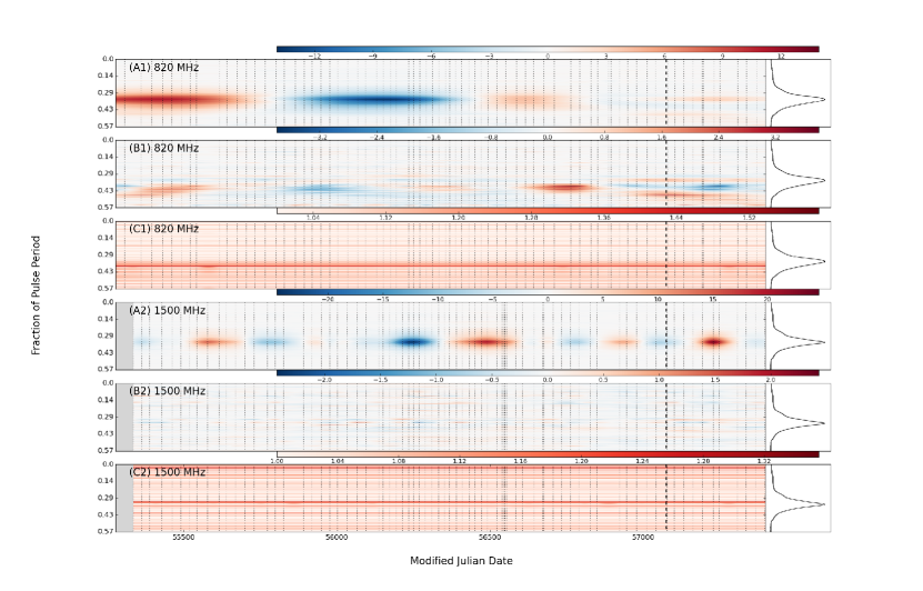
Figure 10: Variability maps for PSR J1643$-$1224. Otherwise as Figure 3.

5 Discussion

We have used a new profile alignment technique, GP regression and multiple metrics to characterize the pulse profile evolution of 78 NANOGrav MSP data sets. All pulsars show flux density variations due to DISS and RISS. After flux density levels are normalized, the differences between the constant average model (for a particular data set) and the observed profiles for most of the pulsars is consistent with being due to additive white Gaussian noise; for the vast majority of pulsars, the mean standard deviation of their on-pulse phase bins is less than a factor of two greater than that of their off-pulse bins. The three pulsars for which this factor is greatest are PSRs J1713$+$0747, B1937$+$21 and J2145$-$0750. Additionally, PSR J1643$-$1224 shows significant long-term variability, which has been previously identified.

5.1 Profile and Timing Variability in J1643$-$1224

As mentioned in Section 4.4, around 2015 February 21 (MJD 57074), Shannon et al. (2016) observe both TOA and pulse profile variations in PSR J1643$-$1224. The largest TOA perturbations are at 3100 MHz. They report a change that leaves permanent excess power in the leading edge of the 3100 MHz and 1400 MHz profiles. Their 700 MHz observations show the least amount of timing variation around this date. TOA perturbations that begin around MJD 57074 can also be seen in NANOGrav data at both 820 MHz and 1500 MHz (Figure 11).

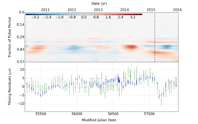
Figure 11: The profile and timing residuals of the J1643$-$1224 820 MHz data set observed at the GBT. The top panel is a variability map showing pulse profile shape changes after the observations have been normalized. Red regions indicate where the inferred pulse profile has an excess of flux density compared to the average for the data set. Blue indicates where it has a deficit. The unit for the variability map is the mean of the standard deviation of the off-pulse phase bins for the data set. This panel depicts the same data as Panel B1 of Figure 10, with the addition of a solid vertical line, which denotes 2015 February 21 (MJD 57074), the date around which timing and profile changes were seen by Shannon et al. (2016). The bottom panel shows the TOA residuals for PSR J1643$-$1224 (Arzoumanian et al., 2018) at 820 MHz (green) and 1500 MHz (blue).

As seen in column 3 of Table 1, however, the PSR J1643$-$1224 1500 MHz pulse profiles are the most stable of all the data sets analyzed in this work. This suggests that the pulse profile changes are not the cause of the TOA disruptions. At 820 MHz, we see more obvious pulse profile changes, but they occur across the whole data set, rather than abruptly around MJD 57074, as seen by Shannon et al. at 3100 MHz. The 820 MHz changes seem to occur primarily at the trailing edge of the profile, which is, again, in contrast to the 3100 MHz Parkes data, in which Shannon et al. see a significant excess signal in the leading edge after $\sim$ MJD 57074, occurring concurrently with a significant change in the timing residuals. At around the same time, the NANOGrav 820 MHz GBT data show a profile feature drifting away from the central peak over a span of a few hundred days (Figure 12). A similar phenomenon occurred in the Crab pulsar in 1997 (Backer et al., 2000), which has been attributed to refraction and multiple imaging at the edge of a plasma cloud in the outer region of the Crab Nebula (Graham Smith et al., 2011).

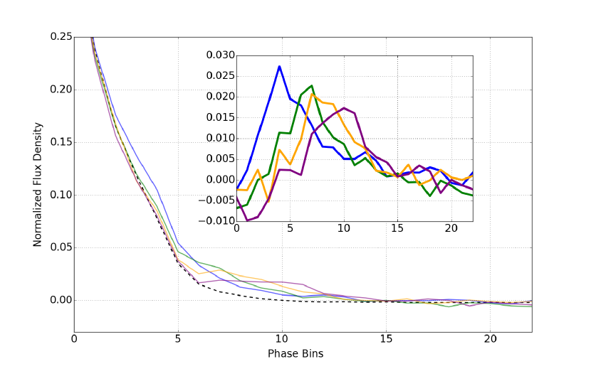
Figure 12: The main plot shows the trailing edge of the pulse profile for PSR J1643$-$1224 observed at 820 MHz. The 2048 phase bins that span the pulse period have been resampled to 64 in order to increase the profile S/N. The average profile for the data set is shown by a black dashed line. The four solid lines are the profiles as observed on MJDs 57102 (blue), 57307 (green), 57336 (orange) and 57369 (purple). The inset shows the difference between each colored profile in the main plot and the average pulse profile (observation minus average). The phase location of the maximum deviation can be seen to drift from left to right with time.

Only profiles at 3100 MHz are shown in the Shannon et al. paper, and so a direct comparison of Parkes and GBT PSR J1643$-$1224 pulse profiles at similar frequencies around the time of the TOA disturbance has yet to been done.

Whenever considering the pulse phase at which profile variability occurs, it should be understood that different methods for alignment can show the variability to occur at different parts of the pulse profile.

5.2 The Effect of Pulse Profile Shape Changes on TOAs

A TOA is determined by a technique that matches the pulse profile from an individual observation, with a static pulse profile model (Taylor, 1992; van Straten, 2006). Any evolution of the pulse profile with time, therefore, will affect the TOA that is produced by this template matching procedure. As discussed in Section 1, in the NANOGrav 11-year data set each frequency subband is used to produce TOAs via the template matching procedure. It should be stressed, therefore, that there are phenomena that could cause profile changes in the frequency-integrated pulse profiles, but have little effect on the profiles of individual frequency channels and, therefore, on the NANOGrav TOAs.

In order to assess the magnitude of changes in TOA that result from the frequency-integrated pulse profile shape variability that we have seen, we employ the template matching procedure using the PYPULSE software package (Lam, 2017). The fitPulse function performs the template matching procedure described in Taylor (1992); any two pulse profiles are cross-correlated in order to calculate a difference in TOA between them.

Before the template matching analysis was carried out, the relative alignment of the pulse profiles was performed. We have employed a new, objective pulse profile alignment technique that maximizes the number of pulse phase bins that are in agreement between profiles (see Section 3.1 for details). The nature of the alignment technique is such that we are insensitive to phase shifts caused by astrophysical processes such as timing noise. In this paradigm, the definition of the fiducial point (a reference point for timing measurements) becomes the phase at which the pulse profile has the least variability; without knowledge of the physical processes involved in the profile shape changes, we assert that this is a reasonable thing to do. In some cases, the profile shape change is quite dramatic and consequently has a dramatic effect on the TOA, as calculated in Table 2. The mean and standard deviations in the table may be dominated by such outliers and be skewed as a consequence. The metric of $\left<|\Delta\rm{TOA}|\right>$ and standard timing residuals are difficult to compare; we are not using traditional pulsar timing. Instead we are instead essentially assuming that the pulsar is a perfect rotator and have defined the fiducial point as the most stable phase of the pulsar. Additionally, as discussed in Section 3.1, we are only aligning in single bin increments (with 2048 bin resolution) as it is sufficient for the profile profile variability analysis that is the focus of this work. Not aligning to fractions of a phase bin may also inflate the values in Table 2.

Table 2 shows the TOA changes ($\Delta\rm{TOA}$) induced by the pulse profile shape changes seen in PSRs J1643$-$1224, J1713$+$0747, B1937$+$21 and J2145$-$0750. The template model used is the average profile of all normalized observations that survived the analysis in Section 3. A value of $\Delta\rm{TOA}$ was calculated for each observation. Template matching the average model with itself produces a $\Delta\rm{TOA}$ value of zero by definition.

Table 2: The changes in TOA induced by pulse profile variation for PSRs J1643$-$1224, J1713$+$0747, B1937$+$21 and J2145$-$0750.

Pulsar	Observing Frequency (MHz)	$\left<|\Delta\rm{TOA}|\right>$ ($\mu$s)	$\sigma\Delta\rm{TOA}$ ($\mu$s)	Max. $\Delta\rm{TOA}$ ($\mu$s)	$\left<\sigma\rm{TOA}\right>$ (ns)
J1643$-$1244	820	0.75	0.93	5.00	3.44
J1643$-$1244	1500	0.39   0.44	0.34   0.40	1.65   1.86	3.70   3.52
J1713$+$0747	1400	1.37	2.36	12.81	2.50
J1713$+$0747	2030	1.27	1.45	7.40	4.90
J1713$+$0747	1500	0.89   0.88	0.84   0.84	4.94   3.92	2.92   2.90
J1713$+$0747	820	0.92	0.92	5.00	4.21
B1937$+$21	820	0.21	0.15	0.74	0.74
B1937$+$21	1500	0.23   0.17	0.25   0.14	2.08   0.58	0.74   0.64
B1937$+$21	1400	0.16	0.11	0.43	0.84
B1937$+$21	2030	0.22	0.12	0.48	1.88
J2145$-$0750	820	3.26	2.61	10.10	15.26
J2145$-$0750	1500	1.96   1.92	1.33   1.22	5.42   4.12	15.18   16.10

Note. — $\left<|\Delta\rm{TOA}|\right>$ is the mean of the absolute TOA change induced by the pulse profile shape changes. $\sigma\Delta\rm{TOA}$ is the standard deviation of the $\Delta\rm{TOA}$ distribution. Max. $\Delta\rm{TOA}$ is the largest TOA changed induced in the data set, and $\left<\sigma\rm{TOA}\right>$ is the mean uncertainty in the TOA calculations. The data sets observed at 1500 MHz have two values for each variability metric. The left of the pair relates to profiles that were polarization calibrated only by a local noise diode, and the right to profiles that were additionally polarization calibrated using the full Mueller matrix (see Section 3).

In the 12 data sets analyzed, the average value of the magnitude of $\Delta\rm{TOA}$ induced by the changing pulse profile shape is typically around three orders of magnitude larger than the average 1$\sigma$ uncertainty of the TOA measurements $\left<\sigma\rm{TOA}\right>$.

In general, the potential causes of the pulse profile variability are scintillation, inaccurate DM, scatter broadening, instrumental and interference issues, jitter or other emission changes intrinsic to the pulsar. We discuss each possibility in detail in the following.

5.3 Diffractive Interstellar Scintillation (DISS)

DISS is the frequency-dependent modulation of pulsar flux density. If a pulse profile is a composite of a wide range of equally weighted frequency channels (as it is in this analysis), scintillation will necessarily lead to pulse profile changes, providing that (i) the profile evolves with frequency across the observing band, (ii) the scintillation bandwidth is not much smaller than the observing bandwidth and (iii) the scintillation timescale is not much smaller than the timescale of the observation. In each data set for PSRs J1643$-$1224, J1713$+$0747, B1937$+$21 and J2145$-$0750, scintillation is occurring to differing degrees, affecting the relative flux in different parts of the observing band (see Figure 13). There is also some pulse profile shape evolution across the observing band for PSRs J1713$+$0747, B1937$+$21 and J2145$-$0750. Therefore, scintillation plays at least some part in the pulse profile variability seen in the analysis of these three pulsars. Relatively little pulse profile shape evolution is seen across the observing band for PSR J1643$-$1224.

Levin et al. (2016) showed that the average scintillation bandwidth for PSR B1937$+$21 at 1500 MHz is around 2.8 MHz, which is close to the resolution limit. Keith et al. (2013) give a value of 1.2 MHz at a reference frequency of 1500 MHz. The fractional uncertainty in the scintillation bandwidth is $1/\sqrt{N_{iss}}$, where

$$N_{iss}\approx\left(1+\zeta\frac{\Delta\nu}{\Delta\nu_{d}}\right)\left(1+\zeta\frac{T}{\Delta t_{d}}\right),$$ (2)

and where $\zeta$ is an empirically determined coefficient ($\zeta\approx$ 0.1-0.2), $\Delta\nu$ is the receiver bandwidth, $\Delta\nu_{d}$ is the scintillation bandwidth, $T$ is the integration time of the observation and $\Delta t_{d}$ is the scintillation timescale (Cordes et al., 1990). Using $\Delta\nu_{d}=$ 1.2 MHz and $\Delta t_{d}=$ 327 s from Keith et al. (2013) and $\zeta=$ 0.2, the fractional uncertainty in scintillation bandwidth for a 30 minute, 800 MHz bandwidth observation is $\sim$ 6% For the 1400 and 2030 MHz centered observations in this analysis, the observing bandwidth is 800 MHz, for 1500 MHz it is 700 MHz and for the 820 MHz centered observations it is 200 MHz. As these bandwidths are so much larger than the scintillation bandwidths for PSR B1937$+$21, we expect to see scintillation effects largely averaging out across the observing band. Figure 13 shows that although the scintillation observed in PSR B1937$+$21 is much less than that observed in PSRs J1713$+$0747 and J2145$-$0750, the relative weighting of different parts of the observing band does change with time.

Levin et al. were unable to calculate the scintillation bandwidth for PSR J1643$-$1224, limited by the frequency resolution of their observations. Keith et al. (2013) give a value of 22 kHz at a reference frequency of 1500 MHz. Using Equation 2, setting $\Delta\nu_{d}$ to 22 kHz and $\Delta t_{d}$ to 582 s from Keith et al. and setting $\zeta$ to 0.2, gives a scintillation bandwidth fractional uncertainty for a 30 minute, 800 MHz bandwidth observation of $\sim$ 1%. Again, these observing bandwidths are so much larger than the scintillation bandwidth, we expect to see scintillation effects averaging out across the observing band. Despite this, the top panel of Figure 13 indicates that scintillation is causing some changes in the relative flux density across the observing band for PSR J1643$-$1224.

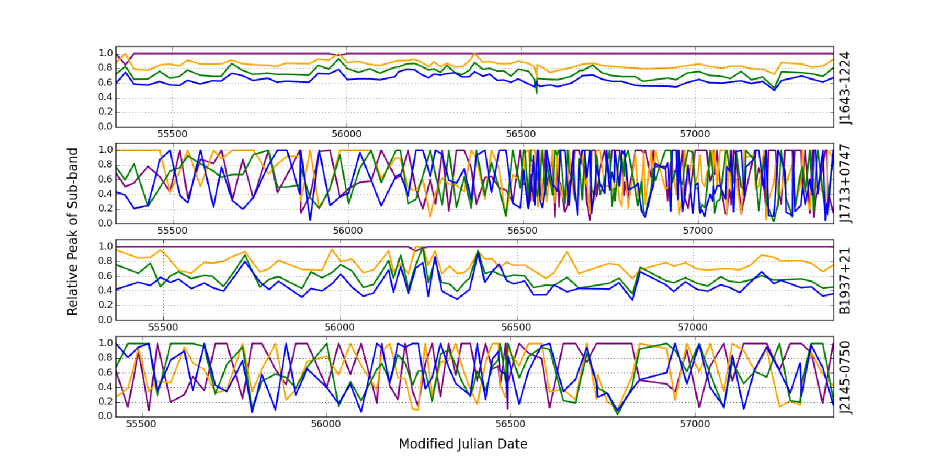
Figure 13: The relative brightness of frequency subbands within the observing band at 1500 MHz. The $\sim$ 800 MHz bandwidths are divided into four $\sim$ 200 MHz bandwidths. From lowest to highest frequency, the subbands are represented by purple, orange, green and blue. From top to bottom, the panels show the relative subband brightness for PSRs J1643$-$1224, J1713$+$0747, B1937$+$21 and J2145$-$0750.

The average scintillation bandwidth reported at 1500 MHz by Levin et al. is 21.1 MHz for PSR J1713$+$0747 and 47.8 MHz for PSR J2145$-$0750. The second to top and bottom panels in Figure 13 indicate clear scintillation for PSRs J1713$+$0747 and J2145$-$0750 respectively.

Figure 14 illustrates the nature of typical pulse profile variations that we see in the PSR J2145$-$0750 data set at 820 MHz. The figure shows that when divided into four $\sim$ 50 MHz frequency bands, the pulse profile shapes of the subbands are largely stable between MJDs 55361 and 56792 (see Panels B2 and C2) and the relative flux densities are not (see Panels B1 and C1). Between these two observation dates, the relative weighting of parts of the observing band has been changed by scintillation. As the different parts of the band have different profile shapes, a modification of the frequency-integrated pulse profile necessarily results. The pulse profile changes that are seen in PSR J2145$-$0750 are, therefore, consistent with the effects of scintillation.

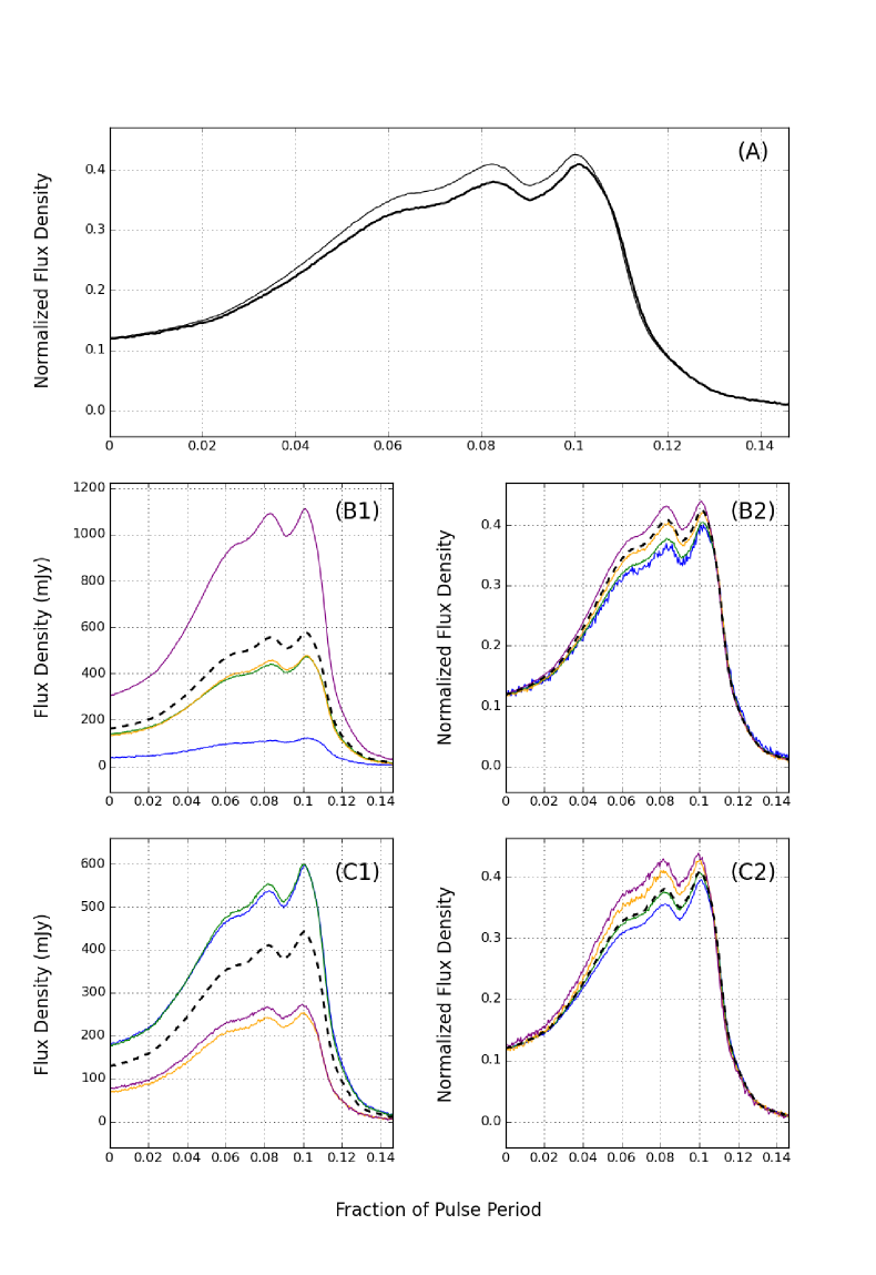
Figure 14: Two contrasting pulse profiles of PSR J2145$-$0750 at 820 MHz. Panel A shows two pulse profiles aligned and normalized by their peaks. The peak is not shown; all panels focus only on a subsection of the profile. This is done to allow shape changes to be seen clearly. The thin line is the pulse profile as observed on MJD 55361 and the thick line on MJD 56792. Panel B1 shows the MJD 55361 observation split into four frequency subbands, each spanning 50 MHz. From lowest to highest frequency, the subbands are represented by purple, orange, green and blue profiles. The black dashed line shows the frequency-integrated profile. In Panel B2, the subband and frequency-integrated profiles have also been normalized to, and aligned by, the peak. Panel C1 and C2 show the same as B1 and B2 respectively, but for the observation made on MJD 56792.

For PSRs J1643$-$1224, J1713$+$0747 and B1937$+$21, some variability is not consistent with the effects of scintillation. In Figure 15, the pulse profile variations centered at 820 MHz are seen to correlate across the observing band for both PSR J1643$-$1224 and PSR B1937$+$21. We do not expect such effects to be the result of scintillation. Figure 16 shows that the systematic pulse profile variability of PSR J1713$+$0747 at 1500 MHz is seen in only two of the four frequency subbands.

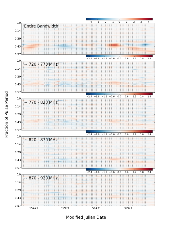
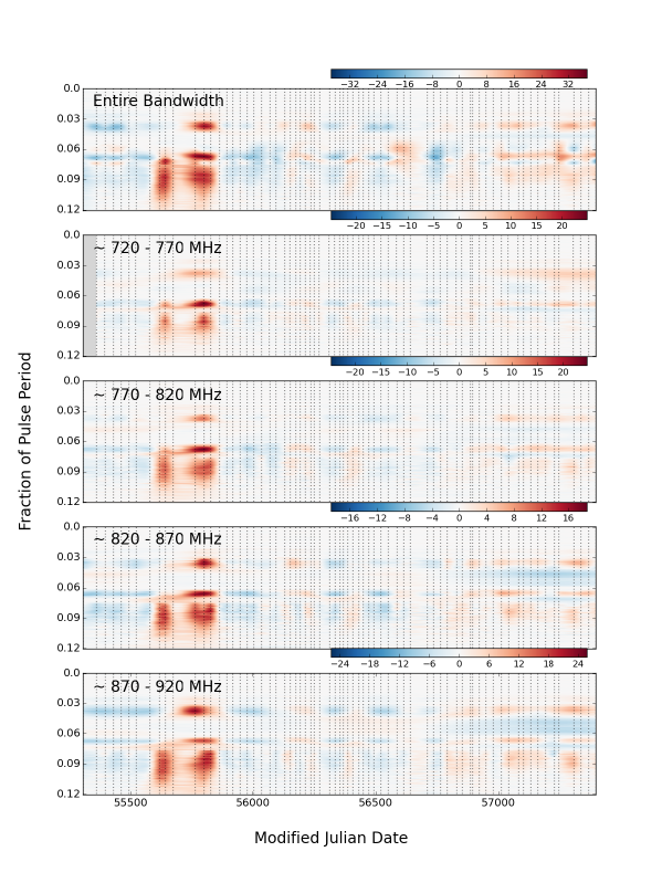
Figure 15: Variability maps for GUPPI data sets broken down into subbands of observational frequency. The left panel panel shows observations of PSR J1643$-$1224 with a central frequency of $\sim$ 820 MHz. The right panel shows the same for PSR B1937$+$21. The unit for all panels is the mean of the standard deviation of the off-pulse phase bins for the relevant subband data set. Otherwise as Figure 3.

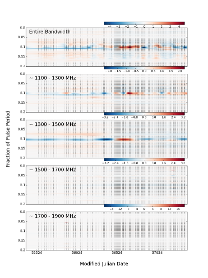
Figure 16: Variability maps for PSR J1713$+$0747 GUPPI observations at a central frequency of $\sim$ 1500 MHz, broken down into subbands of observational frequency. The unit for all panels is the mean of the standard deviation of the off-pulse phase bins for the relevant subband data set. Otherwise as Figure 3.

Furthermore, for some observations, we see that the evolution of the pulse profile across the observing band, is different than for others. An example in PSR J1713$+$0747 can be seen by comparing panels B2 and C2 in Figure 17. It is not clear how such differences could be caused by scintillation.

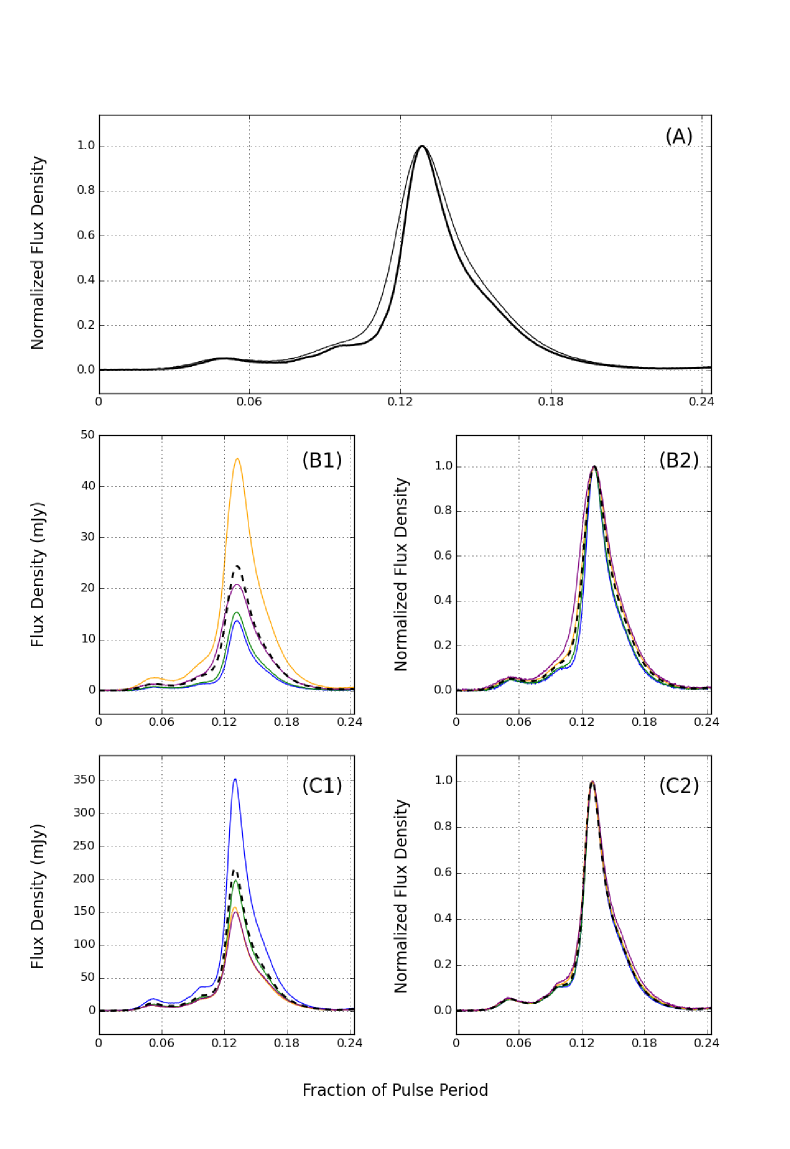
Figure 17: Two contrasting pulse profiles of PSR J1713$+$0747 at 1400 MHz. Panel A shows two pulse profiles aligned and normalized by their peaks. This is done to allow shape changes to be seen clearly. The thin line is the pulse profile as observed on MJD 56360 and the thick line on MJD 57076. Panel B1 shows the MJD 56360 observation split into four frequency subbands, each spanning 200 MHz. From lowest to highest frequency, the subbands are represented by purple, orange, green and blue profiles. The black dotted line shows the frequency-integrated profile. In Panel B2, the subband and frequency-integrated profiles have also been normalized to and aligned by the peak. Panel C1 and C2 show the same as B1 and B2 respectively, but for the observation made on MJD 57076. We see from Panels B2 and C2 that the evolution of the pulse profile across the observing band, is different for the two observations.

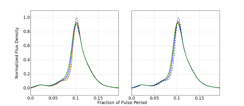
Figure 18: How the frequency-integrated pulse profiles of PSR J1713$+$0747 change with DM at 1400 MHz. Left panel: The black dashed profile was dedispersed at a DM of 15.990 pc cm^-3. The orange, blue and green profiles were dedispersed with 0.04, 0.06 and 0.08 pc cm^-3 added respectively. Right panel: Three observations in the data set showing large deviations from the average pulse profile. The black dashed profile is the average for the data set. The orange, blue and green profiles were recorded on MJDs 56360, 56598 and 57239 respectively.

5.4 Inaccurate DM

As an electromagnetic signal travels though the IISM, its interaction with free electrons produces a frequency-dependent time delay that scales as $\nu^{-2}$ where $\nu$ is the signal frequency. The magnitude of this delay is proportional to the integrated column density of electrons along the path of the signal, which is known as the DM. If we fail to correct for such frequency dependent time delays, an integrated pulse profile that is created by summing a signal detected across a range of observing frequencies, will necessarily appear smeared out when compared to the intrinsic pulse shape. Although correcting for such signal dispersion is routine, DMs are well known to vary with epoch both systematically and stochastically (Keith et al., 2013; Lam et al., 2016a; Jones et al., 2017) due primarily to a changing line of sight. NANOGrav measures the value of DM at nearly every observing epoch (Arzoumanian et al., 2015), but an inaccurate DM value can lead to a modified pulse profile.

Because NANOGrav calculates TOAs for all frequency channels, a further complication is added to the determination of DM. Pulse shapes vary with frequency, but only a single standard template is used in the template-matching procedure. This produces small systematic frequency-dependent perturbations in the TOAs in addition to the $\nu^{-2}$ offsets due to dispersion. To compensate for this, an additional timing delay is added to all timing models, where

$$\Delta t_{\rm{FD}}=\sum c_{i}\mathrm{log}\left(\frac{\nu}{\mathrm{1GHz}}\right)^{i}$$ (3)

and the coefficients $c_{i}$ are fit parameters in the timing model (Arzoumanian et al., 2015). When finding the best-fit timing model parameters for a pulsar, DM and $\Delta t_{\rm{FD}}$ are somewhat covariant, and so the best-fit DM value can change significantly, dependent on whether $\Delta t_{\rm{FD}}$ is included in the timing model.

For the purposes of creating the frequency-integrated pulse profiles employed in this variability analysis, we have calculated the best-fit DM parameters without the inclusion of the $\Delta t_{\rm{FD}}$ parameters that are necessary for TOA determination in individual frequency channels. This minimizes smearing when generating the frequency-integrated pulse profiles.

Jones et al. (2017) report that PSR J1713$+$0747 has a DM of $\sim$ 16 pc cm^-3, which is typically seen to vary on the order of $10^{-4}$ pc cm^-3 on approximately yearly timescales. A 1400 MHz observation that has a DM inaccuracy of a few $10^{-4}$ pc cm^-3 would only introduce a delay across an 800 MHz bandwidth of a few tenths of a microsecond. A single phase bin in our analysis of PSR J1713$+$0747 covers an order of magnitude more time than this (2.23 $\mu$s). Figure 18 demonstrates that to produce some of the most modified pulse profiles in the 1400 MHz data set, the DM would have to be incorrect by the order of $10^{-2}$ pc cm^-3, which is around a hundred times larger than the DM variations that we observe for this pulsar.

PSR B1937$+$21 is calculated to have a DM of $\sim$ 71 pc cm^-3, which is typically seen to vary on the order of $10^{-3}$ pc cm^-3 on approximately yearly timescales. A 1400 MHz observation that has a DM inaccuracy of a few $10^{-3}$ pc cm^-3 would introduce a delay across an 800 MHz bandwidth of a few microseconds. This is the equivalent of a few PSR B1937$+$21 phase bins (each spanning 0.76 $\mu$s). Figure 19 shows that to produce some of the profile variations seen in the 820 MHz data set, the DM would have to change by around $10^{-3}-10^{-2}$ pc cm^-3, which is comparable to the typical DM fluctuations seen in this pulsar.

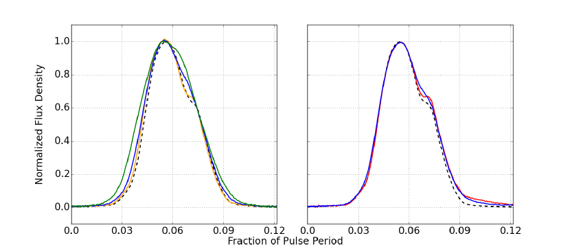
Figure 19: How the frequency-integrated pulse profiles of PSR B1937$+$21 change with DM at 820 MHz. Left panel: The black dashed profile was dedispersed at a DM of 71.025 pc cm^-3. The orange, blue and green profiles were dedispersed with 0.005, 0.01 and 0.015 pc cm^-3 subtracted respectively. Right panel: Two observations in the data set showing large deviations from the average pulse profile. The black dashed profile is the average for the data set. The red profile was recorded on MJD 55641 and the blue on MJD 55765.

A DM of 62.4 pc cm^-3 with approximately yearly fluctuations of around $10^{-3}$ pc cm^-3 is reported for PSR J1643$-$1224 by Jones et al.; an incorrect DM value of this magnitude would introduce a delay at 820 MHz across an 200 MHz bandwidth of a few microseconds. This is the equivalent of one or two PSR J1643$-$1224 phase bins (each spanning 2.26 $\mu$s). However, the phase drifts that are seen in Figure 12 are not suggestive of profile changes induced by incorrect DM measurements, as the modifications in each observation are localized in relatively narrow regions of pulse phase; a more smeared effect would be expected from incorrect DM values.

PSR J2145$-$0750 has a DM of 9 pc cm^-3 with typical variations on the order of $10^{-3}$ pc cm^-3 occurring on approximately yearly timescales as reported by Jones et al.; inaccuracies on this scale would introduce a delay of a few microseconds across the 200 MHz bandwidth at 820 MHz. This is only a fraction of a J2145$-$0750 phase bin which spans $\sim$ 8 $\mu$s. Additionally, even in the most deviant pulse profiles in the data set, some sharp features remain, which would be smeared out when a DM inaccuracy (of the magnitude needed to replicate the profile changes) exists.

Based on these calculations, an inaccurate (but realistic) DM value used to dedisperse the pulsar signal when producing a frequency-integrated pulse profile could produce shape changes in PSRs B1937$+$21 and J1643$-$1224, but is unlikely to produce those observed in PSR J1713$+$0747 or J2145$-$0750.

5.5 Temporal Broadening from Scattering

Electromagnetic waves traveling through the IISM are scattered and follow different paths to the observer. This can, therefore, lead to the broadening of an observed pulse profile; an intrinsically narrow pulse will broaden due to scattering, producing an exponential decay of the pulse with a characteristic timescale $\tau$ known as the scattering timescale. Scatter broadening is a frequency-dependent effect, with $\tau\propto\nu^{-4.4}$ for a thin screen scattering model (Cordes & Lazio, 1991).

Levin et al. (2016) determine average scattering timescales via the measurement of scintillation bandwidths $\Delta\nu$ in the dynamic spectra of the observations, using the relationship

$$2\pi\Delta\nu\tau\sim 1,$$ (4)

(Cordes & Rickett, 1998). For PSR B1937$+$21, Levin et al. calculate that at 1500 MHz, the average $\tau$ is around 44 ns. This is close to the limit imposed by the frequency resolution of their observations. For some epochs, therefore, no scintillation bandwidth could be measured, meaning only a lower limit for $\tau$ on the order of tens of nanoseconds could be inferred. At 820 MHz, these values translate to scattering timescales on the order of a microsecond or more. Cordes et al. (1990) measure the scattering timescale at 430 MHz for the main pulse of PSR B1937$+$21 to be 25$\pm$2 $\mu$s and 30$\pm$2 $\mu$s for the interpulse. Assuming a thin screen scattering model, this translates to a $\tau$ value of a few microseconds at 820 MHz. At 327 MHz, Ramachandran et al. (2006) measure 120 $\mu$s with an rms variation of 20 $\mu$s. With the thin screen scattering assumption, 120 $\mu$s at 327 MHz translates to approximately 3 $\mu$s at 820 MHz. Keith et al. (2013) give a scintillation bandwidth of 1.2 MHz for PSR B1937$+$21, which translates to a scattering timescale of approximately 1.8 $\mu$s at 820 MHz. We simulate the effects of thin screen scatter broadening by convolving a pulse profile with a one-sided exponentially decaying function. We use a one-sided exponential function as an approximation to the pulse broadening function caused by interstellar scattering. Actual pulse broadening functions are more rounded at the origin due to the finite thickness of a scattering screen and can have more slowly decaying tails if there is a wide range of scattering length scales, as with a Kolmogorov medium. In Figure 20, such a simulation of scatter broadening for PSR B1937$+$21 shows that if the nature and magnitude of the pulse profile shape changes we see in the 820 MHz data set were produced by thin screen scatter broadening, then $\tau$ would have to be on the order of microseconds, which is consistent with the findings of Levin et al., Cordes et al., Ramachandran et al. and Keith et al. This translates to a scintillation bandwidth less than 1 MHz. Additionally, the strongly correlated variability seen between the main pulse and the interpulse of PSR B1937+21 (most clearly illustrated at 820 MHz in Panel B1 of Figure 5 and Figure 6), is consistent with what would be expected from a scatter broadened signal (or one modified by propagation effects in general). However, a similar effect could also result from global changes in the pulsar magnetosphere, and so intrinsic variability cannot be ruled out on this basis.

For PSRs J1713$+$0747 and J2145$-$0750, Levin et al. (2016) find that $\tau$ is on the order of ns at 1500 MHz. These scattering timescales are much too small for scatter broadening to significantly affect the pulse profile shapes.

The nature of the pulse profile shape changes observed in PSR J1643$-$1224 cannot be well replicated simply by the convolution of a one-sided decaying exponential function; the phase range over which the profile is modified is usually relatively narrow and is also seen to drift with time. However, IISM structure that is close to the line of sight, could permit such transient profile components via the deflection of radio waves back to the observer. Such behavior has been seen previously in other pulsars (Backer et al., 2000; Michilli et al., 2018).

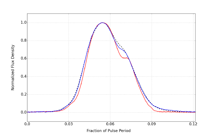
Figure 20: A scatter broadening simulation for PSR B1937$+$21. The red line is the 1400 MHz AO pulse profile observed at MJD 55361, and the blue profile was observed on MJD 55828. The black dashed line is the result of a convolution of the red profile and a one-sided exponential function, in order to simulate the effects of scatter broadening. The $\tau$ value of the exponential function is 9.1 $\mu$s.

5.6 Instrumental Issues & Radio-Frequency Interference

The pulse profile shape changes of PSR J1713$+$0747 at 2030 MHz seem to mainly occur approximately between the MJDs of 57083 (2015 March 2) and 57263 (2015 August 29), as shown in Figure 21.

Figure 21: All 36 pulse profiles of PSR J1713$+$0747 observed at 2030 MHz included in the variability analysis. The red profiles were observed on or between MJDs 57083 and 57263. All other profiles are black.

During this time there are various observations in which the shape of the frequency-integrated profiles and all of the contributing subbands is modified with respect to the average profile shape of the data set. Additionally, during this period there is a large fraction of observations in which the absolute fluxes are recorded as much larger than expected. The S/N of these observations suggests that the high flux density is due to miscalibration rather than a very bright signal. Both of these phenomena are shown on MJD 57108 in Figure 22. The high concentration of pulse profile changes during this time period, along with their nature, may suggest an non-astrophysical cause.

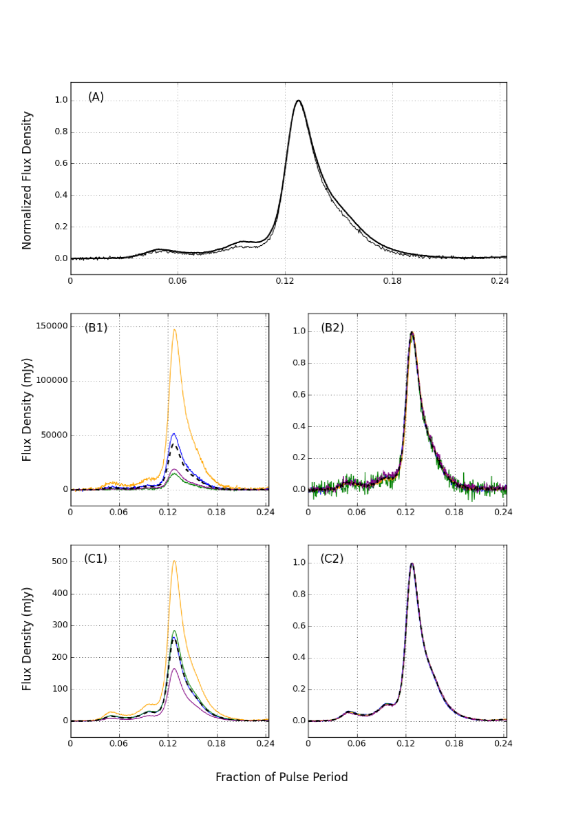
Figure 22: Two contrasting pulse profiles of PSR J1713$+$0747 at 2030 MHz. The thin line in Panel A and Panels B1 and B2 show the observation made on MJD 57108. The thick line and Panels C1 and C2 show the observation made on MJD 57375. The plots are as Figure 17 otherwise. A comparison of Panels B2 and C2 shows that shape of the frequency-integrated profiles and all of the contributing subbands is different for the two observations. This is most noticable at a pulse phase fraction $\sim$ 0.10. The absolute flux in Panel B1 is recorded as much larger than expected.

This hypothesis is bolstered by the fact that in the 2030 MHz observations of PSR B1937$+$21, the most significant pulse profile variations also occur within this date range, as can be seen in Panel B4 of Figure 5 and also in Figure 7. When analyzing all pulsar observations that appeared in the 2030 MHz data set of PSR B1937$+$21 before any profiles were removed due to low S/N, three out of the four highest flux density observations fell within this MJD 57083–57263 range. The absolute fluxes of these observations are very large, with profile peaks around 27, 44 and 65 Jy, yet all have comparatively low S/N, as was the case for PSR J1713$+$0747. This span of time coincides with an era of particularly high levels of RFI around 2000 MHz at AO. The RFI was eventually mitigated by a new filter installed by the observatory in October 2015. As part of the processing, extra RFI removal was carried out for all PUPPI 2030 MHz data before MJD 57300. Much of the frequency band had to be removed from many of these observations, but residual effects of the RFI may well remain and be responsible for the AO profile changes at 2030 MHz.

Further information regarding the cause of these profile changes is provided when comparing the 2030 MHz PSR B1937$+$21 profiles occurring in the MJD 57083-57263 range (discussed above; Figure 7) with Figure 23.

Figure 23: Pulse profile deviations from PSR B1937$+$21 1500 MHz GBT observations that seem to result from incorrect polarization calibration. The solid line shows the average profile for the data set. The dashed profile is an MJD 55977 observation which has had noise diode polarization calibration applied. This discrepancy is not present when full Mueller matrix calibration is employed.

As discussed in Section 2, only the 1500 MHz GUPPI data has undergone two parallel methods of polarization calibration: using a noise diode and the more sophisticated full Mueller matrix calibration. This data set, therefore, gives us an opportunity to see how the different calibration techniques affect the resulting pulse profiles (see also Gentile et al., 2018). Only relatively subtle changes are produced by the different polarization calibration methods for most observations. However, there are some observation days that show large pulse profile variability when calibrated using only the noise diode. One such day is MJD 55977. Figure 23 shows the pulse profile modifications that take place in the PSR B1937$+$21 1500 MHz noise diode calibrated observations made on that day. These deviations from the average all but disappear when full Mueller matrix calibration is applied. The same phenomenon is seen on the same day for PSR J1713$+$0747.

The PUPPI 2030 MHz profiles that fall in the problematic MJD 57083-57263 range and are highlighted in Figure 7, are very similar in nature to the GUPPI 1500 MHz MJD 55977 profile that was polarization calibrated using only a noise diode, both in the main pulse and the interpulse. It is likely, therefore, that the 2030 MHz PSR B1937$+$21 PUPPI profiles highlighted in Figure 7 are also the result of incorrect polarization calibration. Extrapolating further, the PSR J1713$+$0747 2030 MHz PUPPI profile changes that also occur in the same problematic date range as the PSR B1937$+$21 2030 MHz PUPPI observations may also be due to incorrect polarization calibration. The polarimetric calibration of some NANOGrav MSPs is addressed in detail in Gentile et al. (2018). As discussed in Section 2, Gentile et al. have performed full Mueller matrix polarization calibration for the PUPPI data. This is done using a method called Measurement Equation Template Matching (van Straten, 2013), a technique that uses pulsars with known polarization profiles to act as standard sources in order to generate polarimetric responses for any epoch of observation. Unfortunately, the standard sources used by Gentile et al. were PSRs J1713$+$0747 and B1937$+$21. The polarization profiles for these two pulsars are, therefore, assumed to be unchanging and so are not calculated for each observation. In general, Gentile et al. find that the polarimetric responses of AO’s 1400 and 2030 MHz receivers vary significantly with time.

In general, it is possible that some pulse profile shape changes are the result of flux and polarization calibration issues. As discussed in Section 4.1, the flux density calibration procedure was not undertaken correctly for the 1400 MHz AO observation of PSR J1713+0747 made on MJD 56360; an incorrect pulsed calibration signal was injected at the epoch of observation. It is not clear whether the change in pulse profile shape was affected by this, as pulse profiles with similar shapes were also seen in the data set, for which no such calibration issues were seen (MJDs 56598 and 57239).

The profile shape changes of PSR J1643$-$1224 have now been observed by both the GBT and the Parkes Radio Telescope and, therefore, an instrumental cause can be ruled out.

5.7 Jitter

Pulsars are known to exhibit stochastic, broadband, single-pulse variations that are intrinsic to the pulsar emission process and affect the shape of the integrated pulse profile. This phenomenon is known as jitter and contributes noise to the TOAs. Cordes & Downs (1985) showed that on timescales ranging from one pulse period to integrations of up to an hour, TOA variations exceed what is expected from radiometer noise alone in long-period pulsars. Studies of MSPs show similar findings (e.g. Shannon et al., 2014), and this is generally true for NANOGrav MSPs (Lam et al., 2016b).

As jitter is expected to be uncorrelated from one pulse period to the next, it should not be responsible for any systematic profile changes such as those seen in PSRs B1937$+$21 and J1643$-$1224 at 820 MHz. Using the AO 1400 MHz receiver, Shannon & Cordes (2012) studied the impact that jitter has on the timing stability of PSR J1713$+$0747. They predict that for a 30 minute observation (comprising $\sim 10^{5.6}$ pulses), jitter will produce a scatter $\sigma_{\rm{J}}$ in the arrival times of $\sim$ 40 ns. Similarly, Lam et al. (2016b) calculate $\sigma_{\rm{J}}$ for pulsars in the NANOGrav nine-year data set and find values for PSR J1713$+$0747 that range from 39 ns in the AO 1400 MHz data to 91 ns in the GBT 820 MHz data. They find $\sigma_{\rm{J}}$ for PSR B1937$+$21 to be between 5.7 ns (AO 1400 MHz) and 32 ns (GBT 820 MHz). For PSR J2145$-$0750, $\sigma_{\rm{J}}$ is calculated to be 89 ns at 820 MHz and 120 ns at 1500 MHz using GBT data. These values are much smaller than the changes in TOA induced by the observed changes in pulse profile, as seen in Table 2. This indicates that pulse jitter is not the dominant source of the profile changes we observe in PSRs J1713$+$0747, B1937$+$21 and J2145$-$0750. Furthermore, many other pulsars observed by the NANOGrav collaboration show evidence of more jitter noise but less profile shape variability.

Lam et al. (2016b) calculate $\sigma_{\rm{J}}$ for PSR J1643$-$1224 as 162 and 219 ns at 820 and 1500 MHz respectively. This is the same order of magnitude as the changes in TOA induced by the observed changes in pulse profile (Table 2). However, the drifting and systematic nature of the profile changes in the data set is not indicative of jitter, which is uncorrelated in time.

5.8 Other Pulsar Emission Changes

Some pulse profile variability observed in PSRs J2145$-$0750 and B1937$+$21 is consistent with effects of the propagation of a radio signal through the IISM; scintillation and scatter broadening respectively. Some profile modulations in PSRs J1713$+$0747 and B1937$+$21 may also be the product of improper polarization calibration. Other pulse profile shape changes elude a comprehensive explanation and so emission changes intrinsic to the pulsar (besides jitter) cannot be ruled out.

As described above, the changes in PSR J1643$-$1224 profile do not seem to be characteristic of modulations induced by propagation effects, inaccurate DMs, jitter or instrumental issues. As pointed out by Shannon et al. (2016), the drifting nature of pulse profile disturbances is reminiscent of that seen in PSR J0738$-$4042; a pulsar displaying simultaneous changes in emission and rotation, which were assessed to be intrinsic to the neutron star (Brook et al., 2014).

We also note here that PSR B1937$+$21 is known to emit giant pulses (Cognard et al., 1996). The longitude at which the giant pulses are seen to occur is not consistent with the pulse profile shape changes that we see. Additionally, the profile variability in PSR B1937$+$21 occurs on timescales of hundreds of days; no such timescale is known for giant pulse activity.

In general, there are few obvious correlations between the profile shape changes and pulsar flux density (as seen by comparing the A and B prefixed panels in the variability maps). The notable exception is the period between MJDs 57083 and 57263 at 2030 MHz in PSRs J1713$+$0747, B1937$+$21, as discussed in Section 5.6.

Other links between the profile variability and the rotational behavior of a pulsar may provide further clues regarding the source of any variability. Figure 24 shows the behavior of both profile and timing residuals for PSR B1937$+$21. The profile residuals shown are at an observing frequency of 820 MHz (the data set displaying the most systematic variability). A more detailed analysis of any relationship between the emission and rotational properties of these pulsars will be left to future work.

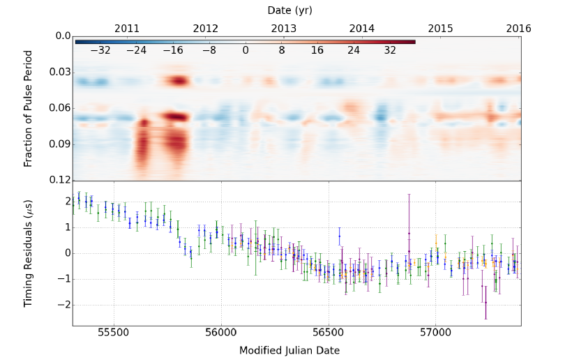
Figure 24: The 820 MHz profile residuals and the timing residuals of B1937$+$21, observed at the GBT. The top panel is a variability map showing pulse profile shape changes after the observations have been normalized and depicts the same data as Panel B1 of Figure 5. Red regions indicate where the inferred pulse profile has an excess of flux density compared to the average for the data set. Blue indicates where it has a deficit. The unit for the variability map is the mean of the standard deviation of the off-pulse phase bins for the data set. The bottom panel shows the TOA residuals for PSR B1937$-$21 at 820 MHz (green), 1400 MHz (orange), 1500 MHz (blue) and 2030 MHz (purple).

Whatever the cause of unmodeled pulse profile changes, they are detrimental to the template matching technique of TOA determination and, therefore, to pulsar timing. For PSRs J1643$-$1224, J1713$+$0747, B1937$+$21 and J2145$-$0750 the TOA inaccuracies induced due to some changes in pulse profile are on the order of hundreds of nanoseconds to microseconds. The frequency-integrated pulse profile changes that we have focused on may not translate to profile changes in the narrow individual frequency channels that the NANOGrav collaboration uses to produces its TOAs however; pulse profiles that result from the combination of a relatively wide band of frequency channels are far more sensitive to shape changes induced by the effects of signal propagation. It is also important that highly aberrant pulse profiles that appear in a data set have their corresponding TOAs removed in order to ensure that the most accurate timing models are produced.

When looking at figures that show the phase location of profile variability, we must be cognizant of the fact that different methods for alignment will show the variability to occur at different parts of the pulse profile. Different alignment methods, however, should largely be in agreement regarding the amount of variability that is contained within a data set, even if they disagree on the phases at which it occurs. A priori, we expect the magnitude of profile variability to be most around the profile peak if we assume that the amount of variability will be proportional to the profile intensity at the phase at which it occurs.

When quantifying the variability seen in pulse profiles, we have discounted the number of pulsar rotations that contribute to the observations. With its very short period of 1.56 ms, the PSR B1937$+$21 data sets typically have around 10⁶ rotations per observation. Conversely, PSR J2145$-$0750 has the longest period of all pulsars analyzed in this work at 16.05 ms. Consequently, the data sets for this pulsar have only around 10⁵ rotations per observation. All else being equal, 10 times more pulses contributing to an integrated pulse profile would increase the S/N by approximately $\sqrt{10}$ and would also decrease the pulse profile variability due to jitter, thereby decreasing the variability measured. Falling in between these extremes, PSRs J1643$-$1224 and J1713$+$0747 have pulse periods of 4.62 and 4.57 ms respectively and so rotate approximately 3-4$\times$10⁵ times per observation.

In future work, MSP pulse profile variability information could lead to the mitigation of timing aberrations caused by the unmodeled pulse profile changes we observe. For example, more NANOGrav data are currently undergoing full Mueller matrix polarization calibration; we have shown that this process can correct pulse profile shape distortions that may result from imperfect calibration when using only a local noise diode. In the case of a pulsar in which pulse profile variability is primarily due to temporal broadening from scattering, we can apply techniques such as cyclic spectroscopy to recover the intrinsic pulse profiles (Demorest, 2011; Walker et al., 2013) from the effects of interstellar scattering. In these two examples, as the differences between the shape of the observed profiles and the timing template are reduced, so too are the timing residuals. If profile shape changes are entirely due to DISS, then the consequences for timing can be minimized by calculating the TOAs for relatively narrow frequency subbands, as is already done by NANOGrav.

To create the smooth, continuous variability maps seen throughout this paper, we have inferred the behavior of the flux density for each phase bin (and, therefore, of the pulse profile as a whole) between observations using GP regression. For pulsars that show systematic variability, such modeling techniques would also permit the extrapolation of pulse profiles shapes. A predicted profile shape could then be used as a dynamic template for the TOA calculation. Using an accurate template shape (if one can be calculated) will necessarily also improve the accuracy of the TOA recorded. For pulsars with more erratic shape changes and less systematic variability, such extrapolations will be difficult to make. However, throughout this analysis, we have also used a new pulse profile alignment technique which maximizes the number of pulse phase bins that are in agreement (see Section 3.1 for details). As a result, only the stable parts of the pulse profiles are used in their alignment. Using only these stable phase bins in the template matching procedure could potentially result in reduced timing residuals for some pulsar data sets.

The question of how the variability measured in this work will impact the predicted timeline for nanohertz gravitational wave detection is a difficult one. Relatively little research has been done on long-term pulse profile variability in MSPs. The physical origin of much of the emerging profile variability is uncertain, can be different for each data set analyzed and must be a mixture of multiple effects to varying degrees. Mitigation of profile variability will require further investigation and, therefore, it is not clear how soon we will be able to accommodate such profile changes in a pulsar timing model. As evidence for MSP profile variability grows, so too will the voicing of suggestions that precision pulsar timing should not be done using the standard template matching techniques, but instead, using other techniques that are more accommodating to such variability, e.g. the profile domain pulsar timing analysis of Lentati et al. (2015). Such discussions make the analyses in this paper more interesting and relevant.

6 Conclusions

The primary aim of this work was to analyze the long-term pulse profile behavior in the 11-year data set employed by the NANOGrav collaboration to search for nanohertz frequency gravitational waves; significant profile variability is detrimental to the effort if overlooked.

PSRs J1713$+$0747, B1937$+$21 and J2145$-$0750 show the highest levels of variability of the pulsars analyzed, with PSR B1937$+$21 showing significant long-timescale trends. These pulsars are also three of the brightest observed by the NANOGrav collaboration. This is not entirely surprising as any pulse profile shape changes are more easily classified as such in bright pulsars, and also, the variability metric is in units of the rms levels of the off-pulse regions, which will be relatively small in such pulsars. Despite this, some of the profile changes seen in these pulsars are of a magnitude that means they would also be visible in pulsars with a much lower S/N; the method used for detecting long-term variability has been shown to be able to do so down to a level that is comparable in magnitude to the rms of the observation noise (Brook et al., 2016). Systematic variability is also observed in the PSR J1643$-$1224 data, which has been identified previously in observations by the Parkes radio telescope. The cause is not yet clear beyond being astrophysical in nature. The variability seen in PSR J2145$-$0750 is consistent with scintillation effects. Some of the profile modification seen in PSRs J1713$+$0747 and B1937$+$21 is likely due to improper polarization calibration and in the 2030 MHz AO observations, RFI is suspected to have strongly influenced some of the changes. However, some variability in B1937$+$21 also seems consistent with scatter broadening, while some profile changes in PSRs J1713$+$0747 are due to effects of scintillation.

In the future, the impact of pulse profile variability on precision timing can be minimized by techniques such as full Mueller matrix polarization calibration, cyclic spectroscopy, the employment of dynamic templates in the template matching procedure and timing to the most stable parts of a pulse profile.

7 Acknowledgements

The NANOGrav project is supported by NSF Physics Frontiers Center award PHYS-1430284. P.R.B. is supported by Track I award OIA-1458952. The Green Bank Observatory is a facility of the National Science Foundation operated under cooperative agreement by Associated Universities, Inc. The Arecibo Observatory is operated by SRI International under a cooperative agreement with the NSF (AST-11000968), and in alliance with the Ana G. Méndez-Universidad Metropolitana, and the Universities Space Research Association. Pulsar research at the University of British Columbia is supported by an NSERC Discovery Grant and by the Canadian Institute for Advanced Research. J.A.E. was partially supported by NASA through Einstein Fellowship grant PF4-150120. W.W.Z. is supported by the CAS Pioneer Hundred Talents Program and the Strategic Priority Research Program of the Chinese Academy of Sciences Grant No. XDB23000000. Portions of this work performed at NRL were supported by the Chief of Naval Research.

Appendix A A Variability Map Demonstrating a Stable Pulse Profile Shape

For illustrative purposes, we present in Figure 25, a variability map for a pulsar that has a stable pulse profile.

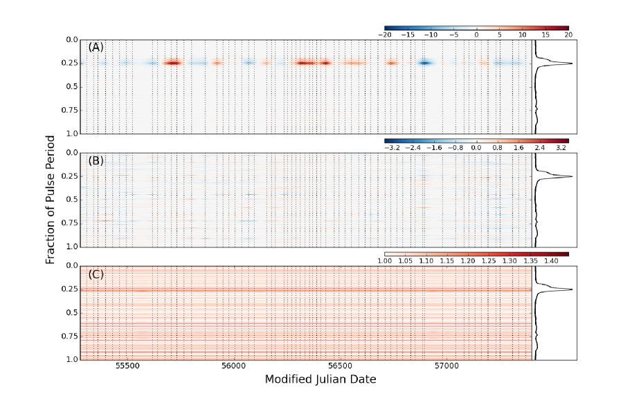
Figure 25: A variability map for a data set in which the pulse profile shape is relatively stable. Panel A shows the flux density variations in the flux-calibrated, pre-normalized observations of PSR J1614$-$2230 at 820 MHz. The flux density variations are due to refractive and diffractive scintillation. Red regions indicate where the inferred pulse profile has an excess of flux density compared to the average for the data set. Blue indicates where it has a deficit. Most variability is seen around the peak of the profile at a pulse period fraction of $\sim$ 0.25. Panel B shows any pulse profile shape changes after the observations have been normalized. As any variability in this data set is consistent with additive white Gaussian noise, the variability map is almost entirely devoid of color; in each phase bin, the GP model lies around zero, i.e. the mean of the data points which inform it. Panel C shows the standard deviation of the inferred GP model as a function of pulse phase and time. The unit for all panels is the mean of the standard deviation of the off-pulse phase bins for the data set. In Panel C the value is close to unity across the whole pulse profile; the variance of the data is approximately the same whether looking at on- or off-pulse phase bins. The vertical dotted lines indicate the epochs of observation informing the GP models. To the right of each panel, the average pulse profile for the data set is shown.

References

- Armstrong (1984) Armstrong, J. W. 1984, Nature, 307, 527
- Arzoumanian et al. (2015) Arzoumanian, Z., Brazier, A., Burke-Spolaor, S., et al. 2015, ApJ, 813, 65
- Arzoumanian et al. (2018) —. 2018, ApJS, 235, 37
- Backer (1970a) Backer, D. C. 1970a, Nature, 228, 42
- Backer (1970b) —. 1970b, Nature, 228, 1297
- Backer et al. (1982) Backer, D. C., Kulkarni, S. R., Heiles, C., Davis, M. M., & Goss, W. M. 1982, Nature, 300, 615
- Backer et al. (2000) Backer, D. C., Wong, T., & Valanju, J. 2000, ApJ, 543, 740
- Brook et al. (2014) Brook, P. R., Karastergiou, A., Buchner, S., et al. 2014, ApJ, 780, L31
- Brook et al. (2016) Brook, P. R., Karastergiou, A., Johnston, S., et al. 2016, MNRAS, 456, 1374
- Camilo et al. (2012) Camilo, F., Ransom, S. M., Chatterjee, S., Johnston, S., & Demorest, P. 2012, ApJ, 746, 63
- Cognard et al. (1995) Cognard, I., Bourgois, G., Lestrade, J.-F., et al. 1995, A&A, 296, 169
- Cognard et al. (1996) Cognard, I., Shrauner, J. A., Taylor, J. H., & Thorsett, S. E. 1996, ApJ, 457, L81
- Cordes & Downs (1985) Cordes, J. M., & Downs, G. S. 1985, ApJS, 59, 343
- Cordes & Lazio (1991) Cordes, J. M., & Lazio, T. J. 1991, ApJ, 376, 123
- Cordes & Rickett (1998) Cordes, J. M., & Rickett, B. J. 1998, ApJ, 507, 846
- Cordes et al. (1990) Cordes, J. M., Wolszczan, A., Dewey, R. J., Blaskiewicz, M., & Stinebring, D. R. 1990, ApJ, 349, 245
- Demorest (2011) Demorest, P. B. 2011, MNRAS, 416, 2821
- DuPlain et al. (2008) DuPlain, R., Ransom, S., Demorest, P., et al. 2008, in Proc. SPIE, Vol. 7019, Advanced Software and Control for Astronomy II, 70191D
- Ford et al. (2010) Ford, J. M., Demorest, P., & Ransom, S. 2010, in Proc. SPIE, Vol. 7740, Software and Cyberinfrastructure for Astronomy, 77400A
- Gentile et al. (2018) Gentile, P. A., McLaughlin, M. A., Demorest, P. B., et al. 2018, ApJ, 862, 47
- Graham Smith et al. (2011) Graham Smith, F., Lyne, A. G., & Jordan, C. 2011, MNRAS, 410, 499
- Heiles et al. (2001) Heiles, C., Perillat, P., Nolan, M., et al. 2001, PASP, 113, 1274
- Helfand et al. (1975) Helfand, D. J., Manchester, R. N., & Taylor, J. H. 1975, ApJ, 198, 661
- Hobbs (2013) Hobbs, G. 2013, Classical and Quantum Gravity, 30, 224007
- Hotan et al. (2005) Hotan, A. W., Bailes, M., & Ord, S. M. 2005, ApJ, 624, 906
- Jones et al. (2017) Jones, M. L., McLaughlin, M. A., Lam, M. T., et al. 2017, ApJ, 841, 125
- Karastergiou et al. (2011) Karastergiou, A., Roberts, S. J., Johnston, S., et al. 2011, MNRAS, 415, 251
- Kaspi et al. (1994) Kaspi, V. M., Taylor, J. H., & Ryba, M. F. 1994, ApJ, 428, 713
- Keith et al. (2013) Keith, M. J., Coles, W., Shannon, R. M., et al. 2013, MNRAS, 429, 2161
- Kramer (1998) Kramer, M. 1998, ApJ, 509, 856
- Kramer & Champion (2013) Kramer, M., & Champion, D. J. 2013, Classical and Quantum Gravity, 30, 224009
- Kramer et al. (2006) Kramer, M., Lyne, A. G., O’Brien, J. T., Jordan, C. A., & Lorimer, D. R. 2006, Science, 312, 549
- Lam (2017) Lam, M. T. 2017, PyPulse, Astrophysics Source Code Library, , , ascl:1706.011
- Lam et al. (2016a) Lam, M. T., Cordes, J. M., Chatterjee, S., et al. 2016a, ApJ, 821, 66
- Lam et al. (2016b) —. 2016b, ApJ, 819, 155
- Lentati et al. (2015) Lentati, L., Alexander, P., & Hobson, M. P. 2015, MNRAS, 447, 2159
- Levin et al. (2016) Levin, L., McLaughlin, M. A., Jones, G., et al. 2016, ApJ, 818, 166
- Lorimer et al. (2012) Lorimer, D. R., Lyne, A. G., McLaughlin, M. A., et al. 2012, ApJ, 758, 141
- Lyne et al. (2010) Lyne, A., Hobbs, G., Kramer, M., Stairs, I., & Stappers, B. 2010, Science, 329, 408
- Lyne et al. (1971) Lyne, A. G., Smith, F. G., & Graham, D. A. 1971, MNRAS, 153, 337
- Lyne et al. (2017) Lyne, A. G., Stappers, B. W., Freire, P. C. C., et al. 2017, ApJ, 834, 72
- Manchester et al. (2013) Manchester, R. N., Hobbs, G., Bailes, M., et al. 2013, PASA, 30, e017
- McLaughlin (2013) McLaughlin, M. A. 2013, Classical and Quantum Gravity, 30, 224008
- Michilli et al. (2018) Michilli, D., Hessels, J. W. T., Donner, J. Y., et al. 2018, MNRAS, 476, 2704
- Pennucci et al. (2014) Pennucci, T. T., Demorest, P. B., & Ransom, S. M. 2014, ApJ, 790, 93
- Ramachandran et al. (2006) Ramachandran, R., Demorest, P., Backer, D. C., Cognard, I., & Lommen, A. 2006, ApJ, 645, 303
- Rasmussen & Williams (2006) Rasmussen, C. E., & Williams, C. K. I. 2006, Gaussian Processes for Machine Learning (Cambridge, MA: MIT Press)
- Rathnasree & Rankin (1995) Rathnasree, N., & Rankin, J. M. 1995, ApJ, 452, 814
- Rickett (1990) Rickett, B. J. 1990, ARA&A, 28, 561
- Roberts et al. (2012) Roberts, S., Osborne, M., Ebden, M., et al. 2012, Philosophical Transactions of the Royal Society of London A: Mathematical, Physical and Engineering Sciences, 371, 1984
- Shannon & Cordes (2010) Shannon, R. M., & Cordes, J. M. 2010, ApJ, 725, 1607
- Shannon & Cordes (2012) —. 2012, ApJ, 761, 64
- Shannon et al. (2013) Shannon, R. M., Cordes, J. M., Metcalfe, T. S., et al. 2013, ApJ, 766, 5
- Shannon et al. (2014) Shannon, R. M., Osłowski, S., Dai, S., et al. 2014, MNRAS, 443, 1463
- Shannon et al. (2016) Shannon, R. M., Lentati, L. T., Kerr, M., et al. 2016, ApJ, 828, L1
- Stairs et al. (2000) Stairs, I. H., Lyne, A. G., & Shemar, S. L. 2000, Nature, 406, 484
- Taylor (1992) Taylor, J. H. 1992, Philosophical Transactions of the Royal Society of London A: Mathematical, Physical and Engineering Sciences, 341, 117
- Taylor et al. (1975) Taylor, J. H., Manchester, R. N., & Huguenin, G. R. 1975, ApJ, 195, 513
- van Straten (2004) van Straten, W. 2004, ApJS, 152, 129
- van Straten (2006) —. 2006, ApJ, 642, 1004
- van Straten (2013) —. 2013, ApJS, 204, 13
- Walker et al. (2013) Walker, M. A., Demorest, P. B., & van Straten, W. 2013, ApJ, 779, 99