Improved indirect control of nuclear spins in diamond NV centers

Abstract

Hybrid quantum registers consisting of different types of qubits offer a range of advantages as well as challenges. The main challenge is that some types of qubits react only slowly to external control fields, thus considerably slowing down the information processing operations. One promising approach that has been tested in a number of cases is to use indirect control, where external fields are applied only to qubits that interact strongly with resonant excitation pulses. Here we use this approach to indirectly control the nuclear spins of an NV center, using microwave pulses to drive the electron spin, combined with free precession periods optimized for generating logical gate operations on the nuclear spins. The scheme provides universal control and we present two typical applications: polarizing the nuclear spin and measuring nuclear spin free induction decay signals, both without applying radio-frequency pulses. This scheme is versatile as it can be implemented over a wide range of magnetic field strengths and at any temperature.

I Introduction

Hybrid quantum systems kurizki2015quantum , such as electron-nuclear spins of the nitrogen vacancy (NV) center in diamond Suter201750 , have emerged as useful physical systems for implementing quantum computing and imaging nielsen ; Stolze:2008xy ; ladd2010quantum ; blencowe2010quantum ; cai2014hybrid . The difference in the inherent properties of the two subsystems are often useful, e.g. for implementing fast gate operations on the electron spin and achieving long information storage in the nuclear spin. However, it also provides challenges for the coherent control of hybrid spin systems, e.g. since the interaction between the nuclear spin magnetic moment and the control fields is orders of magnitude weaker than that of the electron spins, which has relatively short coherence times.

The magnetic moment of the nuclear spin can be enhanced by the hyperfine coupling with the electron spin in the NV center Suter201750 ; PhysRevB.94.060101 . This corresponds to an enhancement in the effective gyromagnetic ratio of the nuclear spin and is determined by the strength of the coupling. For systems with sufficiently strong couplings, like those of the nearest ¹³C spins to the NV center PhysRevB.94.060101 ; PhysRevA.87.012301 ; PhysRevLett.102.210502 , or the ¹⁴N spin in the NV center dobrovitski2012 ; cnotN15 ; chen15 , the enhancement results in nuclear spin Rabi frequencies that are high enough for direct control of the nuclear spins by the application of radio-frequency fields. However, the enhancement and thus the usefulness of the nuclear spins as qubits decreases dramatically with increasing distance of the nuclear spin from the NV center.

To alleviate this problem, the approach relying on indirect control of the nuclear spins was developed theoretically PhysRevA.76.032326 ; PhysRevA.91.042340 and experimentally demonstrated in various systems, like the malonic acid radical PhysRevA.78.010303 ; PhysRevLett.107.170503 and NV centers PhysRevLett.109.137602 ; naturephoton ; PhysRevB.96.134314 ; Pan13 . This scheme does not require any radio-frequency pulses and therefore achieves much faster operations on the nuclear spins. Instead, it uses only microwave (MW) pulses acting on the electron spin, combined with free precession under the effect of anisotropic hyperfine interactions. The anisotropic interactions result in different orientations of the nuclear spin quantization axes for different states of the electron spin, and provide the possibility to achieve indirect control of the nuclear spin by only controlling the electron spin PhysRevA.76.032326 ; PhysRevA.78.010303 . The basic idea of this scheme is to start with the electron spin initialized, e.g., in the $m_{S}=0$ state and the nuclear spin aligned along the corresponding quantization axis, which is close to the $z$-axis. If a MW pulse changes the state of the electron spin on a timescale that is fast compared to the precession period of the nuclear spin, the nuclear spin remains unchanged during the MW pulse. After the pulse, it is therefore oriented at a nonzero angle from the new quantization axis and starts to precess. The control procedure then consists in finding the best combination of precession periods around the different axes that bring the spin close to the targeted orientation. The control efficiency can be improved by maximizing the angle between the different quantization axes of the nuclear spin PhysRevA.76.032326 .

In our present work, we chose a system where the hyperfine couplings are close to the Larmor frequency of the nuclear spin, which optimizes the difference in the orientation of the quantization axes to a value close to $90^{\circ}$. Moreover, unlike the scheme in PhysRevA.76.032326 , we generalized the switched control scheme by replacing the $180^{\circ}$ pulses by arbitrary operations implemented through pulses with variable flip angles and phases. Such generalization extends the search space for optimizing the pulse sequence parameters, and is useful to improve the control efficiency, e.g., to reduce the number of pulses. In our work, the elementary unitary operations consist of only 2 - 3 rectangular MW pulses separated by delays. Compared to earlier works based on dynamical decoupling naturephoton ; PhysRevB.96.134314 or modulated microwave pulses PhysRevA.78.010303 ; PhysRevLett.107.170503 that used hundreds or even thousands of MW pulse segments, this is a dramatic reduction of the control cost.

In this article, we use this scheme to implement operations that occur in many quantum information or imaging tasks: we generate and detect nuclear spin coherence, transfer population between the electronic and nuclear spins and generate a pseudo-Hadamard gate on the nuclear spin. Using these operations, we polarize the nuclear spin and measure the nuclear spin transition frequencies using free induction decay (FID) signals. Our system of interest consists of the electron spin and one ¹³C nuclear spin, which is relatively weakly coupled to the electron ($A$<0.2 MHz). In this system, the nuclear spin transition frequencies (NMR spectrum) are spread over a spectral range of more then 200 kHz, which would be out of reach for direct radio-frequency excitation but can be readily excited by our indirect control scheme.

II System and operations to implement

The spin system consists of the electron, the ¹⁴N nuclear spin and one ¹³C nuclear spin. In this context, we do not consider the ¹⁴N spin but focus on the subsystem where the ¹⁴N is (and remains) in the $m_{N}$=1 state. The spins interact with a weak magnetic field $B$ oriented along the symmetry axis of the NV-center. In a suitable reference frame (for details see Appendix A), we can write the relevant part of the Hamiltonian as

$$\frac{\mathcal{H}_{e,C}}{2\pi}=DS_{z}^{2}-(\nu_{e}-A_{N})S_{z}-\nu_{C}I_{z}+A_{zz}S_{z}I_{z}+A_{zx}S_{z}I_{x},$$

where $S_{z}$ denotes the electron spin-1 operator, and $I_{x/z}$ the ¹³C spin-1/2 operators. The zero-field splitting is $D=2.87$ GHz and $\nu_{e/C}=\gamma_{e/C}B$ denote the Larmor frequencies of the electron and ¹³C nuclear spins and $\gamma$ the gyromagnetic ratios. $A_{N}=-2.16$ MHz is the secular part of the hyperfine coupling with the ¹⁴N nuclear spin while $A_{zz}$ and $A_{zx}$ are the relevant components of the ¹³C hyperfine tensor.

The eigenstates of $\mathcal{H}_{e,C}$ are $|1,\varphi_{+}\rangle,|1,\psi_{+}\rangle,|0,\uparrow\rangle,|0,\downarrow\rangle,|-1,\varphi_{-}\rangle$, and $|-1,\psi_{-}\rangle$, where $|\uparrow\rangle$ and $|\downarrow\rangle$ are the eigenstates of $I_{z}$,

$$|\varphi_{\pm}\rangle = |\uparrow\rangle\cos(\theta_{\pm}/2)+|\downarrow\rangle\sin(\theta_{\pm}/2)$$

$$|\psi_{\pm}\rangle = -|\uparrow\rangle\sin(\theta_{\pm}/2)+|\downarrow\rangle\cos(\theta_{\pm}/2)$$ (1)

are the nuclear-spin eigenstates and

$$\theta_{\pm}=\arctan\frac{A_{zx}}{A_{zz}\mp\nu_{C}}$$ (2)

are the angles between the nuclear spin quantization axis and the $z$-axis of our coordinate system for the subsystems where the electron spin is in the state $m_{S}=\pm 1$. $|1\rangle$, $|0\rangle$ and $|-1\rangle$ are the eigenstates of $S_{z}$. Additional details are given in Appendix A. The nuclear spin transition frequencies are $\nu_{C}$ and $\nu_{\pm}=\sqrt{A_{zx}^{2}+(\nu_{C}\mp A_{zz})^{2}}$ if the electron spin is in the state $m_{S}=0$, and $m_{S}=\pm 1$, respectively. In the following, we use the eigenstates $\{|0\rangle,|-1\rangle\}\otimes\{|\uparrow\rangle,|\downarrow\rangle\}$ of the operators $S_{z}$ and $I_{z}$ as our computational basis.

The experiments were performed at room temperature. We used a ¹²C-enriched diamond crystal with a ¹³C concentration of $0.002\%$ PhysRevLett.110.240501 ; 1882-0786-6-5-055601 and applied a magnetic field $B=14.8$ mT. We selected a center with a resolved coupling to a ¹³C nuclear spin, with the coupling constants $A_{zz}=-0.152$ MHz and $A_{zx}=0.110$ MHz. For this center, the quantization axis of the nuclear spin is oriented at an angle $\theta_{+}=-10^{{\circ}}$, $\theta_{-}=86^{{\circ}}$ and $\theta_{0}\approx 0$ from the $z$-axis if the electron spin is in the $\pm 1$ or 0 state. The MW pulses had a Rabi frequency of $\approx 0.5$ MHz, which is small compared to $A_{N}$ and to $\nu_{e}$. Accordingly, they only drive the transition from the $m_{S}=0$ to one of the $m_{S}=\pm 1$ states and are selective for $m_{N}=1$.

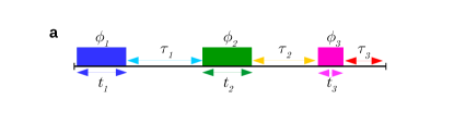
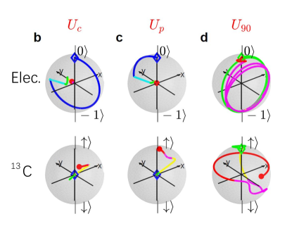
Figure 1: Pulse sequence and Bloch sphere representation for the evolution of the electron- and ¹³C spins. (a) MW pulse sequence at a fixed power with the carrier frequency set to the ESR transition frequency $m_{S}=0\leftrightarrow-1$. The pulse durations, phases and delays are indicated as $t_{k}$, $\phi_{k}$, and $\tau_{k}$ respectively. (b-d) Evolution trajectories of the electron and ¹³C spin on the Bloch sphere under the operations $U_{c}$, $U_{p}$ and $U_{90}$. The initial and final states are indicated by diamonds and filled circles, respectively. In Fig. (b), $U_{c}$ maps $\rho_{0}$ to $\rho_{c}$, corresponding to a mixed electron state and a maximum possible ¹³C coherence. In (c), $U_{p}$ swaps the states between the electron and ¹³C. In (d), the electron and ¹³C spins are both initially in state $|0\rangle$. Under $U_{90}$, the ¹³C spin evolves towards the -$y$-axis, while the electron returns to its initial state. Here $U_{90}$ consists of only 2 MW pulses and 2 delays, i.e., $t_{1}$ =$\tau_{1}$ = 0 in Fig. (a). The color of each partial trajectory corresponds to the color in (a). The parameters of these operations are given in Appendix B. The $x$, $y$ and $z$ components of the final states on the Bloch sphere are presented in Table 4 in Appendix D.

As initial examples of the indirect control approach, we implement three state-to-state transfer operations to which we refer as $U_{c}$, $U_{c}^{\dagger}$ , and $U_{p}$, and one unitary operation, $U_{90}$. The initial state for the first three operations is

$$\rho_{0}=|0\rangle\langle 0|\otimes E/2,$$ (3)

where $E$ is the $2\times 2$ identity operator. This state corresponds to the electron spin in a pure state and the ¹³C nuclear spin in the maximally mixed state.

We first consider the operations $U_{c}$ and $U_{c}^{\dagger}$, where $U_{c}$ converts $\rho_{0}$ into nuclear spin coherence in the manifolds $m_{S}=0$ and $m_{S}=-1$ of the electron spin and $U_{c}^{\dagger}$ transfers the coherence back to population in $m_{S}=0$. The target state of the operation $U_{c}$ is

$$\rho_{c}=U_{c}\rho_{0}U_{c}^{\dagger}=\frac{1}{2}(|0\rangle\langle 0|\otimes|s_{0}\rangle\langle s_{0}|+|-1\rangle\langle-1|\otimes|s_{-}\rangle\langle s_{-}|)$$ (4)

where

$$|s_{0}\rangle = (|\uparrow\rangle+i|\downarrow\rangle)/\sqrt{2}$$

$$|s_{-}\rangle = (|\varphi_{-}\rangle-|\psi_{-}\rangle)/\sqrt{2}$$ (5)

denote superpositions of the nuclear spin in the energy eigenbasis of the manifolds $m_{S}=0$ and $-1$.

$U_{p}$ implements a selective population transfer. It transforms the initial state $\rho_{0}$ to

$$\rho_{p}=U_{p}\rho_{0}U_{p}^{\dagger}=\frac{1}{2}(|0\rangle\langle 0|+|-1\rangle\langle-1|)\otimes|\uparrow\rangle\langle\uparrow|,$$ (6)

where the electron spin is in the maximally mixed state in the subspace $m_{S}=\{0,-1\}$ while the nuclear spin is in the pure state $|\uparrow\rangle$. Clearly $U_{p}$ implements a SWAP operation that aligns the nuclear spin along the $z$-axis.

To implement the operation $U_{c}$, $U_{c}^{\dagger}$ or $U_{p}$, we search for pulse sequence that maximizes the overlap between the final state and the target state. We use a MATLAB^® subroutine based on a genetic algorithm Mitchell:1998:IGA:522098 to find the optimal set of parameters. The third operation $U_{90}=e^{-i(\pi/2)I_{x}}$ is a $\pi/2$ rotation around the $x$-axis for ¹³C, or a pseudo-Hadamard gate, since it is equivalent to the Hadamard gate $U_{H}$ up to operations around the $z$-axis as

$$U_{H}=ie^{-i(\pi/2)I_{z}}U_{90}e^{-i(\pi/2)I_{z}},$$ (7)

where the $z$- rotations can be easily absorbed in a suitable reference frame shift PhysRevLett105200402 ; PRA78012328 . For $U_{90}$, we maximize the process fidelity of the gate. Fig. 1 (a) illustrates the pulse sequence, where the pulse durations $t_{k}$, phases $\phi_{k}$, and the durations $\tau_{k}$ of the free precession periods were used as adjustable parameters in the optimization.

To obtain sequences that are robust against fluctuations of the MW power, we averaged the fidelities over a range of MW field amplitudes, as described in the Appendix B. We obtained theoretical state fidelities of $95\%$ for the target states of $U_{c}$ and $U_{c}^{\dagger}$, and $98\%$ for $U_{p}$ with sequences of 3 pulses and 3 delays, and gate fidelity of $92\%$ for $U_{90}$ with a sequence of 2 pulses and 2 delays. The total duration of these pulse sequences is $\approx 7-15\mu$s, shorter than the transverse relaxation time $T_{2}^{*}\approx 20\mu$s of the electron spin. Figs. 1(b-d) show the evolution of the electron and ¹³C spins during the pulse sequence on the Bloch sphere during these pulse sequences.

III Experimental results

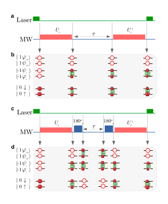
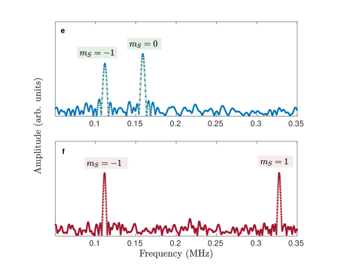
Figure 2: Experimental schemes and results for generating and detecting coherence in ¹³C spin via indirect control. (a, c) Pulse sequences. The red rectangles denote MW pulse sequences resonant with transition $m_{S}=0\leftrightarrow-1$ to implement the operations $U_{c}$ and $U_{c}^{\dagger}$, as indicated above the rectangles. The blue rectangles denote $180^{\circ}$ -pulses resonant with transition $m_{S}=0\leftrightarrow 1$ in the $m_{N}=1$ subspace. The first laser pulse initializes the electron and ¹³C in state $\rho_{0}$. $U_{c}$ transforms $\rho_{0}$ to $\rho_{c}$. $\rho_{c}$ or $\rho_{c}^{\prime}$ then undergoes free evolution for time $\tau$ and $U_{c}^{\dagger}$ transfers the evolved coherence back to population of the $m_{S}=0$ state. During the second laser pulse, photon counting measures this population. (b, d) Schematic representations of the state evolution at each stage of the operation. The filled circles represent the populations and the wavelike patterns represent coherence. (e-f) Spectra of the ¹³C spin, measured with the sequences (a) and (c), respectively. The states of electron spin are indicated in the panels for each resonance line.

The experimental scheme to measure ¹³C transition frequencies via indirect FID measurement in electron subspaces of $m_{S}=\{0,-1\}$, and the pictorial representations of the state evolution are shown in Figs. 2 (a, b). The first laser pulse initializes the system to state $\rho_{0}$. This is followed by the generation of ¹³C coherence using $U_{c}$ as indicated by the wavelike patterns in Fig. 2 (b). $\rho_{c}$ then evolves freely for a time $\tau$. $U_{c}^{\dagger}$ converts the final coherence back to population of $m_{S}=0$. The last laser pulse is used to measure the population of $m_{S}=0$, and generates a signal proportional to

$$P_{|0\rangle}=Tr\{\rho_{c}\rho_{\tau}\}=[\cos(2\pi\nu_{C}\tau)+\cos(2\pi\nu_{-}\tau)]/8+1/4$$ (8)

with $\rho_{\tau}=e^{-i\tau\mathcal{H}_{e,C}}\rho_{c}e^{i\tau\mathcal{H}_{e,C}}$.

Figs. 2 (c-d) show the experimental scheme and state representations for the ¹³C FID in $m_{S}=\{-1,1\}$. It starts with the same sequence as in (a) to put the system in to the state $\rho_{c}$. A first $180^{\circ}$ pulse applied to the $m_{S}=0\leftrightarrow 1$ transition then transforms $\rho_{c}$ into

$$\rho_{c}^{\prime}=(|1\rangle\langle 1|\otimes|s_{0}\rangle\langle s_{0}|+|-1\rangle\langle-1|\otimes|s_{-}\rangle\langle s_{-}|)/2.$$ (9)

In the $m_{S}=1$ state, the nuclear spin quantization axis is almost parallel to the $z$-axis ($\theta_{+}\approx 0^{\circ}$). Therefore, the nuclear spin coherence remains an almost equal weight superposition of the two eigenstates, which subsequently undergoes free evolution for a time $\tau$. After the free evolution, the second $180^{\circ}$ pulse exchanges again the states $m_{S}=1$ and $m_{S}=0$ and $U_{c}^{\dagger}$ works in the same manner as in Fig. 2 (a). The signal generated after the last laser pulse is proportional to

$$P_{|0\rangle}^{\prime}=Tr\{\rho_{c}^{\prime}\rho_{\tau}^{\prime}\}=[\cos(2\pi\nu_{-}\tau)+\cos(2\pi\nu_{+}\tau)]/8+1/4$$ (10)

with $\rho_{\tau}^{\prime}=e^{-i\tau\mathcal{H}_{e,C}}\rho_{c}^{\prime}e^{i\tau\mathcal{H}_{e,C}}$.

Figs. 2 (e-f) show the resulting ¹³C spectra, obtained by Fourier transformation of the FID data which are presented in Fig. 12 in the Appendix D. Since $\rho_{c}$ and $\rho_{c}^{\prime}$ contain coherence in two different NMR transitions, each of the resulting spectra features two resonance lines. The measured transition frequencies are 0.159, 0.111, and 0.328 MHz and agree well with the analytical solutions for $\nu_{C}$, $\nu_{-}$ and $\nu_{+}$ respectively. The linewidths are not the natural linewidths but are determined by the truncation of the FID signal. Since the FID for Fig. 2 (f) was measured for 300 $\mu$s and that for (e) for 200 $\mu$s, the resonance lines in (f) are slightly narrower. More details are presented in Appendix D.

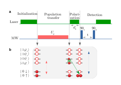
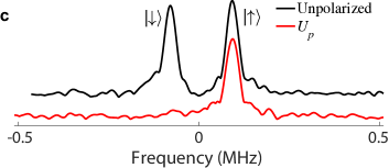
Figure 3: Polarization scheme and experimental results. (a) Pulse sequence. In the initialization step, the electron and ¹³C spins are set into state $\rho_{0}$. For the population transfer, we apply MW pulses to transfer the population from states $|0,\downarrow\rangle$ to $|-1,\uparrow\rangle$. In the polarization step, a laser pulse resets the electron from $m_{S}=-1$ back to $m_{S}=0$. We then measure an electron spin FID on the transition $m_{S}=0\leftrightarrow m_{S}=1$ to determine the populations of the carbon spin states $|\uparrow\rangle$ and $|\downarrow\rangle$. Here we use MW pulses with a Rabi frequency of 3.7 MHz to reduce the operation time, since the selectivity for the subspace of ¹⁴N state is not required. The peaks of other ¹⁴N states are also observed but not shown here. (b) Schematic representation of the state during the intermediate steps in (a). The filled circles denote the population size. The short (long) vertical double arrows indicate the transition $m_{S}=0\leftrightarrow-1$ ($m_{S}=0\leftrightarrow 1$). (c) ESR spectra of the $m_{S}=0\leftrightarrow 1$ transition obtained from states $\rho_{0}$ and $\rho_{p}$ when $d_{L}$ =0, where the ¹³C spin is unpolarized (thermal) and in state$|\uparrow\rangle$, indicated by the black and red curves, respectively.

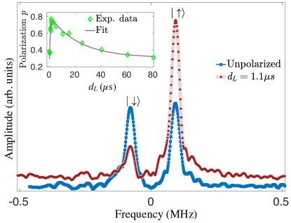
Figure 4: ESR spectra of the $m_{S}=0\leftrightarrow 1$ transition when the ¹³C spin is in the unpolarized state and when it is polarized with a laser pulse of duration $d_{L}=1.1$ $\mu$s resulting in a polarization $p\approx 80\%$. In inset shows the dependence of the population difference $p$ on the laser pulse duration $d_{L}$.

As yet another illustration, we use $U_{p}$ to polarize ¹³C - a necessary step in realizing quantum computation Cramer:2016aa ; PhysRevLett.110.060502 ; Appl.Phys.Lett.105.242402 ; PhysRevA.87.012301 ; NJP19073030 ; arXiv:1806.05881 ; naturephoton ; PhysRevLett.109.137602 . Figs. 3 (a-b) show the experimental scheme and a schematic representation of the states during the intermediate steps. After the initialization step, $U_{p}$ transforms $\rho_{0}$ to $\rho_{p}$, see Eq. (6). The laser pulse in the polarization step resets the electron from $m_{S}=-1$ back to $m_{S}=0$. To measure the populations of states $|0,\uparrow\rangle$ and $|0,\downarrow\rangle$, denoted as $P_{|0\uparrow\rangle}$ and $P_{|0\downarrow\rangle}$, in the $m_{S}=0$ subsystem, we performed the standard FID experiment on the electron spin, followed by a detection laser pulse. In the obtained ESR spectrum, the amplitudes of the resonance lines are proportional to the populations $P_{|0\uparrow\rangle}$ and $P_{|0\downarrow\rangle}$, respectively.

Fig. 3 (c) shows the spectra obtained from $\rho_{0}$ (as a reference) and $\rho_{p}$ ,when the laser pulse in the polarization step was switched off. In the spectrum from $\rho_{p}$, the population of state $|0,\downarrow\rangle$ was almost completely moved away, shown as the negligibly small left peak. Ideally, the right peak should have the same height as in the unpolarized state spectrum. The ratio of the two peak amplitudes is $\approx$0.92, which we use as a measure of the fidelity of the implemented $U_{p}$.

Fig. 4 shows the experiment result for polarizing the ¹³C spin with a laser pulse of duration $d_{L}=1.1$ $\mu$s. The corresponding spectrum for the unpolarized ¹³C spin is also shown as a reference. The inset shows the nuclear spin polarization $p=P_{|0\uparrow\rangle}-P_{|0\downarrow\rangle}$ as a function of the laser pulse duration, for a laser power of about 0.5 mW. It can be fitted by the function

$$p_{repo}=0.31-0.51e^{-(\alpha+\beta)d_{L}}+0.50e^{-2\gamma d_{L}}$$ (11)

where $\alpha=1.10$ $\mu$s^-1, $\beta=0.41$ $\mu$s^-1 and $\gamma=0.022$ $\mu$s^-1 are the pumping rates for states $|-1,\uparrow\rangle\rightarrow|0,\uparrow\rangle$ (or $|-1,\downarrow\rangle\rightarrow|0,\downarrow\rangle$), $|-1,\uparrow\rangle\rightarrow|0,\downarrow\rangle$ (or $|-1,\downarrow\rangle\rightarrow|0,\uparrow\rangle$), and $|0,\uparrow\rangle\leftrightarrow|0,\downarrow\rangle$, respectively PhysRevA.87.012301 . The highest polarization of $p_{max}\approx 80\%$ was reached for a laser pulse duration $d_{L}$ around $1.1\mu$s.

In the following, we use this polarized state to demonstrate the pseudo-Hadamard gate $U_{90}$. We detect its effect by implementing the standard ¹³C FID experiment (see, e.g., PhysRevA.87.012301 ; dobrovitski2012 ). The MW pulse sequences and experimental results are shown in Fig. 5. Unlike in subspace $m_{S}=0$, we replace $U_{90}$ by a $180_{y}^{\circ}$ MW pulse that transforms $m_{S}=0$ to $-1$, and generates a coherence between $|\psi_{-}\rangle$ and $|\varphi_{-}\rangle$ of ¹³C in $m_{S}=-1$ subspace since $\theta_{-}\approx 90^{\circ}$. The scheme for the $m_{S}=1$ subspace is similar to the case of $m_{S}=0$, except that we transfer the spin states between $m_{S}=0$ and $m_{S}=1$ by$180_{y}^{\circ}$ pulses before and after the free evolution time $\tau$. The measured transition frequencies are measured as $0.158$, $0.110$ and $0.328$ MHz, matching well with $\nu_{C}$, $\nu_{-}$ and $\nu_{+}$.

The performance of the operations $U_{c}$ and $U_{90}$ can be evaluated by analyzing the signals shown in Figs. 2 and 5, combined with numerical simulation. The experimental fidelities for $U_{c}$ and $U_{90}$ are $0.91$ and $0.74$, respectively. The details are presented in Appendix C. The theoretical infidelities for the sequences are 0.02, 0.05, and 0.08, for $U_{c}$, $U_{p}$ and $U_{90}$. The excess infidelities can be attributed to relaxation effects of the electron spin and pulse imperfections.

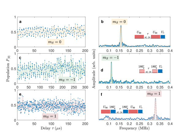
Figure 5: Experimental ¹³C FIDs obtained with the transformation $U_{90}$. The time domain data and the Fourier transforms are shown as the left to right columns. From top to bottom we list the results obtained in the subspaces $m_{S}=0,-1,1$, and the insets show the MW pulse sequences correspondingly. $U_{t}$ performs as a controlled NOT -like gate approximately in the subspace spanned in the basis $\{m_{S}=0,m_{S}=1\}\otimes\{\uparrow,\downarrow\}$ to transfer the population from state $|0,\downarrow\rangle$ to $|1,\downarrow\rangle$Ournewpaper , so that the ¹³C coherence can be detected by the readout laser. $U_{t}$ is implemented by two $90^{\circ}$ MW pulses with $90^{\circ}$ phase shift and separated by a delay of $1/(2|A_{zz}|)$.

IV Discussion

IV.1 The coupled ¹⁴N

Since our interests in the current work focuses on the control of the electron and ¹³C spins, perturbing effects from the ¹⁴N, which is also coupled to the electron spin should be minimized. For this purpose, we have chosen a suitable strength of the MW pulses, such that the Rabi frequency of the MW pulses is strong enough compared with the couplings of the ¹³C, but weak enough to affect only one subspace of the ¹⁴N Ournewpaper . This strategy works well for the case where the couplings of the ¹³C are even weaker, and the MW strength can be further reduced to improve the selectivity for the subspace TranSel . However, for the case where the couplings of the ¹³C are comparable or even higher than the coupling from the ¹⁴N, the selection of the subspace becomes more challenging. For this case, one of the alternatives is to polarize the ¹⁴N PolN14Duan1 ; PolN14Duan2 , e.g., to the state $m_{N}=1$, so that the ¹⁴N only contributes a fixed frequency shift, and high power (or hard) MW pulses can be used. Obviously the effects of the coupled ¹⁴N depend on the achieved polarization of the ¹⁴N. Recent results show that a polarization of$>98\%$ can be reached arXiv:1806.05881 .

We used numerical simulations to investigate the fidelity and duration of the operations $U_{p}$ and $U_{90}$ for different Rabi frequencies. The results are listed in Table 1. For $U_{p}$, the results are not sensitive to the Rabi frequency. For $U_{90}$, higher Rabi frequencies lead to higher fidelities, with similar total sequence length. In these simulations, the pulse sequences are not robust against the fluctuation of the MW power, and therefore the theoretical fidelities at 0.5 MHz Rabi frequency are higher than the robust - sequences used in the experiment.

	$U_{p}$		$U_{90}$
Rabi (MHz)	Fidelity	Duration ($\mu$s)	Fidelity	Duration ($\mu$s)
0.2	0.996	8.65	0.82	13.9
0.5	0.997	7.85	0.97	13.4
10	0.998	7.65	0.99	13.1

Table 1: Simulated results for the dependence of the fidelity and total duration of the operations $U_{p}$ and $U_{90}$ on the Rabi frequency of the MW pulses.

IV.2 Comparison with the previous work

	$U_{p}$		$U_{90}$
Rabi (MHz)	Fidelity	Duration ($\mu$s)	Fidelity	Duration ($\mu$s)
10	0.65	6.5	0.99	13.1
0.5	0.61	10-17	0.97	13.5

Table 2: Results obtained by simulation using the theoretical scheme proposed in Ref. PhysRevA.76.032326 . In the optimization for $U_{p}$ or $U_{90}$, we used the same numbers of the pulses and delays in the pulse sequence shown in Fig. 8, except that we fixed the flip angles for each pulse to $180^{\circ}$.

In previous works based on dynamical decoupling (DD) naturephoton ; PhysRevB.96.134314 , multiple cycles of the DD sequences were applied. The delay time between the DD pulses was determined by DD spectroscopy, and the weak coupling condition was used, where the hyperfine coupling is small compared to the Larmor frequency of the nuclear spin. In our system, however, the Larmor frequency $\nu_{C}$ is close to the hyperfine coupling, violating this condition.

In Ref. Pan13 , the proximal ¹³C spin was studied, where the hyperfine coupling is much larger than the Larmor frequency. In this case, it is possible to generate a large angle between the nuclear quantization axes of the manifolds $m_{S}=0$ and $m_{S}=-1$ by choosing a suitable angle between the static field and the NV axis. The DD pulses were used to flip the states of the electron spin. Compared with this work, the hyperfine coupling in our work is much weaker, and the Rabi frequency of the nuclear spin cannot be observed in our experimental setup.

Using the theoretical procedure outlined in in Ref. PhysRevA.76.032326 , we simulated the short sequences of MW pulses but fixed the flip angle for each pulse to $180^{\circ}$. We checked the optimization for $U_{p}$ and $U_{90}$. The results of the simulation are listed in Table 2. For $U_{p}$, the fidelity is quite low, which indicates that this method does not work for $U_{p}$. For $U_{90}$, however, we obtained useful results as listed in Table 2. These results illustrated the similarity between our pulse opitimization and the switched control in Ref. PhysRevA.76.032326 . Such similarity can also be noticed in the pulse sequence for $U_{90}$ used in the experiment, shown in Fig. 8 in Appendix B , where the flip angles are effectively close to $180^{\circ}$.

IV.3 Number of MW pulses

Using more pulses and delays provides additional parameters for the optimization of the pulse sequences and can therefore result in higher theoretical fidelities. In a typical implementation, however, they lead to longer sequences and therefore aggravate losses of the fidelity through decoherence. Moreover, the additional pulses also introduce additional errors from pulse imperfections. In the present system, we found that sequences with 2-3 pulses are a good compromise.

Using numerical simulations, we investigated the dependence of the fidelity and operation duration on the number of MW pulses. For $U_{90}$, using 3 pulses, we can improve the fidelity to 0.99. This result is consistent with the theoretical prediction PhysRevA.76.032326 . However, the operation duration is about 32 $\mu$s, twice as long as with 2 pulses (see Fig. 8 in Appendix B), and exceeds the transverse relaxation time of the electron spin. The control pulses may thus have to be combined with DD pulses, as illustrated in previous works naturephoton ; PhysRevB.96.134314 ; Pan13 .

The number of pulses that is required to implement a specific operation depends on the angle between the nuclear spin quantization axes in the different electron spin eigenstates. We demonstrate this with a simulation for the present system: if we change the static magnetic field to 28 mT, the ¹³C Larmor frequency becomes 0.3 MHz and the angle $\theta_{-}$ changes to $36.6^{\circ}$, while $\theta_{0}$ does not change. Table 3 lists the results for the operation $U_{p}$ for a Rabi frequency of $\omega_{1}=0.5$ MHz. Here, the optimal number of pulses is 5, which is consistent with the theoretical prediction that number of rotations required is not more than 6 PhysRevA.76.032326 . The pulse sequences are shown as Fig. 9 in Appendix B.

Number of pulses	Fidelity	Duration ($\mu$s)
3	0.86	11.6
4	0.976	13.5
5	0.997	8.89

Table 3: Results of the optimisation of $U_{p}$, for $\theta_{-}=36.6^{\circ}$.

V Conclusion

We have demonstrated highly efficient control of nuclear spins in a solid-state system without using any radio-frequency irradiation. Instead, we relied on suitably chosen sequences of microwave pulses that drive the electronic spin and thereby modulate the anisotropic interaction and the effective field acting on the nuclear spins. The scheme was verified for the example of diamond NV-centers, working at room temperature. Using this technique, we implemented several fundamental unitary operations for quantum computing, such as generating quantum coherence, transferring populations, and Hadamard-like gate. For this demonstration, we only used 2 or 3 MW control pulses, resulting in short gate times. Our scheme does not require a specific choice of the magnetic field, it can be used at arbitrary temperature and applied to different types of hybrid qubit systems.

Acknowledgement This work was supported by the DFG through grants SU 192/34-1 and SU 192/19-2. We thank Daniel Burgarth for helpful discussions .

Appendix

V.1 System, Hamiltonian and ESR Spectra

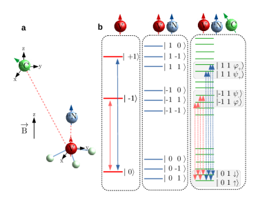
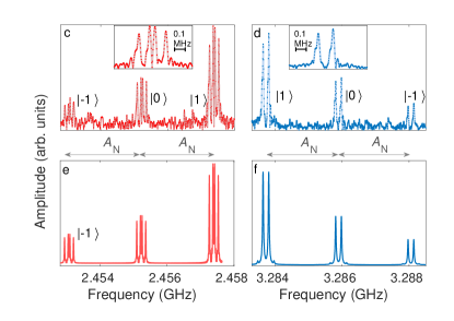
Figure 6: Characteristics of the system. (a) Structure of the NV system with the electron spin coupled to one ¹⁴N and one ¹³C nuclear spin. (b) Energy levels of the system consisting of the electron, ¹⁴N and ¹³C nuclear spins. The vertical double arrows indicate the ESR transitions that we use in this work. (c, d) Experimental ESR spectra obtained in a field of $B=14.8$ mT for the transitions between the $m_{S}=0\leftrightarrow-1$ and $m_{S}=0\leftrightarrow+1$ levels, respectively. The labels $|0\rangle$, $|1\rangle$, and $|-1\rangle$ mark the state of the ¹⁴N spin. The insets show the peaks corresponding to the ¹⁴N state $|1\rangle$ on an expanded scale. The horizontal double arrows indicate the hyperfine coupling with ¹⁴N. The spectra in (e, f) show the matching numerical simulations. The small outer peaks in the simulated spectrum in figure (f) are below the noise levels in the experimental spectrum.

We consider the spin system consisting of the electron, the ¹⁴N nuclear spin and one ¹³C nuclear spin. The axis of the NV system, together with the position of the ¹³C nucleus define a symmetry plane for the system PhysRevB.94.060101 . We therefore use a symmetry-adapted coordinate system, where the $z$-axis is oriented along the NV axis, while the ¹³C nucleus is located in the $xz$-plane, as shown in Fig. 6 (a). The static magnetic field $\overrightarrow{B}$ is aligned along the NV symmetry axis so as to simplify the Hamiltonian and to maximize the electron spin polarization NJPmaxP . The relevant Hamiltonian is then

$$\mathcal{H}/(2\pi) = DS_{z}^{2}-\nu_{e}S_{z}+P(I_{z}^{N})^{2}-\nu_{N}I_{z}^{N}-\nu_{C}I_{z}$$ (12)

$$+ A_{N}S_{z}I_{z}^{N}+A_{zz}S_{z}I_{z}+A_{zx}S_{z}I_{x}.$$

The symbols for the electron spin $\vec{S}$ and the ¹³C nuclear spin $\vec{I}$ are defined in the main text. $I_{z}^{N}$ denotes the spin-1 operator for ¹⁴N, which experiences a nuclear quadrupole splitting with coupling constant $P=-4.95$ MHz and a hyperfine interaction with coupling constant $A_{N}=-2.16$ MHz  PhysRevB.89.205202 ; PhysRevB.47.8816 ; Yavkin16 . Fig. 6 (b-f) show the energy levels and ESR spectra.

If we focus on a subspace where the state of the ¹⁴N is fixed ($m_{N}=1$ in the main text), $\mathcal{H}_{e,C}$ can be diagonalized by the unitary transformation

$$U_{T}=|1\rangle\langle 1|\otimes R_{y}(\theta_{+})+|0\rangle\langle 0|\otimes E+|-1\rangle\langle-1|\otimes R_{y}(\theta_{-}),$$ (13)

where $R_{y}(\theta_{\pm})=e^{-i\theta_{\pm}I_{y}}$. The four ESR transitions $m_{S}=0\leftrightarrow\pm 1$ appear then $D\mp(\nu_{e}-A_{N})$, shifted by

$$\frac{1}{2}(\nu_{\pm}+\nu_{C}),\hskip 2.84544pt-\frac{1}{2}(\nu_{\pm}-\nu_{C}),\hskip 2.84544pt\frac{1}{2}(\nu_{\pm}-\nu_{C}),\hskip 2.84544pt-\frac{1}{2}(\nu_{\pm}+\nu_{C}),$$ (14)

where the upper / lower sign indicates that they are associated with the $m_{S}=\pm 1$ states, respectively. The corresponding transition probabilities are

$$\sin^{2}(\theta_{\pm}/2),\hskip 2.84544pt\cos^{2}(\theta_{\pm}/2),\hskip 2.84544pt\cos^{2}(\theta_{\pm}/2),\hskip 2.84544pt\sin^{2}(\theta_{\pm}/2)$$ (15)

respectively.

V.2 Pulse Sequences

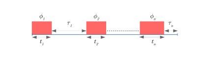
Figure 7: Pulse sequence and variables considered for the numerical search. Here $t_{1},\cdots,t_{n}$ are the durations and $\phi_{1},\cdots,\phi_{n}$ the phases of the MW pulses and $\tau_{1},\cdots,\tau_{n}$ are the delays between them. The amplitude of the pulses is fixed with a Rabi frequency $\omega_{1}/(2\pi)$ = 0.5 MHz.

In a subspace spanned by the states

$$\{|0\rangle,|-1\rangle\}_{e}\otimes\{|1\rangle\}_{N}\otimes\{|\uparrow\rangle,|\downarrow\rangle\}_{C},$$ (16)

the Hamiltonian of the electron-¹³C system can be represented as

$$\frac{1}{2\pi}\mathcal{H}_{s}=(-\nu_{C}-\frac{A_{zz}}{2})I_{z}+A_{zz}s_{z}I_{z}+A_{zx}s_{z}I_{x}-\frac{A_{zx}}{2}I_{x}$$ (17)

in the rotating frame with frequency $D+\nu_{e}-A_{N}$, where $s_{z}$ denotes the pseudo-spin 1/2 operator for electron spin. We consider pulse sequences consisting of $n$ MW pulses with fixed Rabi frequency $\omega_{1}$, as shown in Fig. 7. The propagators for the individual MW pulses can be written as $U_{k}^{MW}=e^{-i\mathcal{H}_{k}^{MW}t_{k}}$ where $\mathcal{H}_{k}^{MW}=\mathcal{H}_{s}+\omega_{1}[s_{x}\cos(\phi_{k})+s_{y}\sin(\phi_{k})]$, and for the free evolutions as $U_{k}^{d}=e^{-i\mathcal{H}_{s}\tau_{k}}$, with $k=\{1,\cdots,n\}$. The total unitary $U$ is a time ordered product of the $U_{k}^{MW}$ and $U_{k}^{d}$, and is a function of the pulse parameters $(t_{1},\cdots,t_{n},\phi_{1},\cdots,\phi_{n},\tau_{1},\cdots,\tau_{n})$. The goal is to design $U$ with suitable pulse parameters such that the fidelity $F_{g}=|\mathrm{Tr(U_{T}^{\dagger}U)}|/4$ of the effective propagator $U$ with respect to the target propagator $U_{T}$ is maximized. We used a genetic algorithm as a numerical search method to obtain the best pulse parameters.

For some applications, we do not have to find a specific unitary propagator, but it is sufficient to transfer a given initial state $\rho_{0}$ to a target state $\rho_{T}$. The actual final state is then $\rho_{opt}=U\rho_{0}U^{\dagger}$, where $\rho_{opt}\equiv\rho_{opt}(t_{1},\cdots,t_{n},\phi_{1},\cdots,\phi_{n},\tau_{1},\cdots,\tau_{n})$, and we maximize the state fidelity $F_{s}=\mathrm{Tr}(\rho_{T}\rho_{opt})/\sqrt{\mathrm{Tr}(\rho_{T}^{2})\mathrm{Tr}(\rho_{opt}^{2})}$.

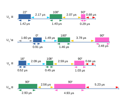
Figure 8: Pulse sequences for $U_{c}$, $U_{c}^{\dagger}$, $U_{p}$ and $U_{90}$ at a fixed $\omega_{1}/(2\pi)$ = $0.5$ MHz. The MW pulses are solid rectangles and are resonant with the ESR transition $0\leftrightarrow-1$. The phases of the pulses are indicated on the top of the rectangles.

The performance of the pulses is sensitive to variations in $\omega_{1}$. To obtain good fidelity in experiments where the actual MW amplitude deviates from the ideal one, we optimized the pulse sequences for a range of amplitudes, taking the average fidelity as the performance measure. For the gates $U_{c}$, $U_{c}^{\dagger}$ and $U_{p}$, we used the range $\omega_{1}/2\pi=[0.47,0.53]$ MHz and for $U_{90}$ $\omega_{1}/2\pi=[0.48,0.52]$ MHz. The optimized pulse sequences for $U_{c}$, $U_{c}^{\dagger}$, $U_{p}$ and $U_{90}$ are shown in Fig. 8. The theoretical robust state fidelities for the four sequences are $95\%$, $95\%$, $98\%$ and $92\%$, respectively.

In Fig. 9, we illustrate a pulse sequence to implement $U_{p}$ for the case of $\nu_{C}=0.3$ MHz, by increasing the static magnetic field.

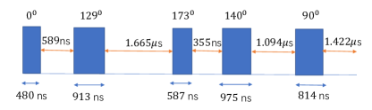
Figure 9: Pulse sequence for $U_{p}$ for $\theta_{-}=36.6^{\circ}$, when $\nu_{C}=0.3$ MHz, at a fixed $\omega_{1}/(2\pi)$ = $0.5$ MHz.

V.3 Experimental performance of $U_{90}$ and $U_{c}$

V.3.1 $U_{90}$

We can exploit the measured populations $P_{|0\rangle}$ shown in Figs. 5 (a), (c) and (e) to estimate experimental fidelity of $U_{90}$. Here we chose the data in initials parts, since the signals in these periods are less noisy. Then we fit the data points using a function as $a_{m_{S}}+b_{m_{S}}\sin(2\pi\nu_{m_{S}}\tau+c_{m_{S}})$, shown in Fig. 10. Here $\nu_{m_{S}}$ denotes the transition frequency measured in the spectra shown in Figs. 5(b, d, f), respectively, with the index indicating the involved subspace. The parameters $a_{m_{S}}$, $b_{m_{S}}$ and $c_{m_{S}}$ are constants in each subspace.

We used the ratios between $b_{m_{S}}$ to estimate the experimental fidelities for $U_{90}$ as well as the $180^{\circ}$ MW pulse in the insets in Figs. 5(d-f) as the following. In this manner, we can eliminate the errors in the operation of polarizing the ¹³C spin and the detection operation $U_{t}$. The fitted $b_{m_{S}}$ is listed as $0.13$, $0.11$ and $0.20$ for $b_{m_{S}}=0$, $1$ and $-1$, respectively. Noticing the pulse sequences shown as the insets in Figs. 5(b) and (f), we can obtain the fidelity for the $180^{\circ}$ MW pulse in the inset (f) as $F_{180}=\sqrt{b_{1}/b_{0}}=0.92$. In a similar way, we then obtained the fidelity for $U_{90}$ as $F_{U_{90}}=\sqrt{b_{1}/b_{-1}}=0.74$. Here we assumed that the the $180^{\circ}$ pulses in insets (d-f) have the same fidelity.

V.3.2 $U_{c}$

In this section, we evaluate the performance of the operation $U_{c}$ using the experimental ¹³C spin spectrum in Fig. 2 (f) measured with the pulse sequence shown in Fig. 2 (c). We then compare this experimental spectrum with the corresponding theoretical spectrum. The theoretical population at the end of this pulse sequence is $P_{|0\rangle}^{{}^{\prime}}$ and its dependence on the delay $\tau$ is explained as Eq. (10) in the main manuscript. The Fourier transformation of $P_{|0\rangle}^{{}^{\prime}}$ in the frequency domain is $y(\nu)=\mathcal{F}\{P_{|0\rangle}^{{}^{\prime}}\}$. We fit this theoretical spectrum to the experimental spectrum by multiplying $y(\nu)$ by a factor $f=0.7$. This fit is shown in Fig. 11. Following this result, we can estimate the experimental fidelity for $U_{c}$ and $U_{c}^{\dagger}$ as $F_{U_{c}}=\sqrt{f}/F_{180}=0.91$, where $U_{c}^{\dagger}$ is assumed the same as $U_{c}$.

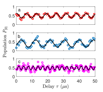
Figure 10: The initial parts of the FIDs shown in Fig. 5, with (a-c) corresponding to Figs. 5 (a), (c) and (e), respectively.

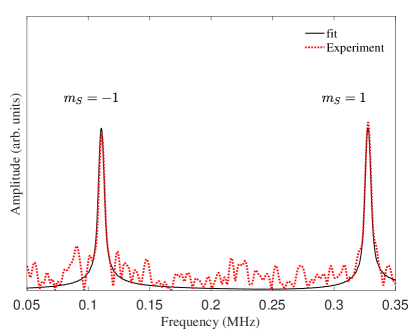
Figure 11: Experimental and theoretical ¹³C spin spectra corresponding to the pulse sequence in Fig. 2(f) of the main text. Here the theoretical spectrum is scaled by a factor of 0.7 to fit the experimental spectra.

V.4 Other supplementary data

In Table 4, we list the components of the final states on the Bloch sphere shown in Fig. 1.

In Figs. 12 (a-b), we illustrated the FID signals of ¹³C obtained by the pulse sequences shown as Figs. 2 (a) and (c), respectively. The corresponding spectra are shown in Fig. 2 (e-f). In experiment we optimized the duration of the FID signal as 200 or 300 $\mu$ for higher S/N. Since the duration of the FID signals is much shorter than both the longitudinal relaxation time of the electron spin ($T_{1}^{e}\approx 3.5$ ms Ournewpaper ), and traversal relaxation time of ¹³C (estimated longer than $T_{1}^{e}$ PhysRevA.87.012301 ), we cannot observe the clear decay of the signals. In the process of Fourier transformation, we added certain window functions and zero filling to improve the spectra. Therefore we cannot observe such relaxation times from the linewidths of the resonance lines in Figs. 2 (e-f).

Operation	Spin	$x$	$y$	$z$
$U_{c}$	Electron	-0.0068	0.1272	0.0008
$U_{c}$	13C	-0.0788	-0.3626	0.4734
$U_{p}$	Electron	0.0004	-0.0016	0.0004
$U_{p}$	13C	0.0698	-0.0608	0.9920
$U_{90}$	Electron	0.0160	-0.0622	0.9690
$U_{90}$	13C	0.1618	-0.9154	0.2810

Table 4: The $x$, $y$ and $z$ components of the final states on the Bloch sphere shown in Fig. 1.

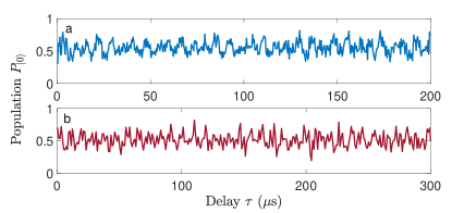
Figure 12: (a-b) ¹³C FID signals obtained by the pulse sequences shown in Figs. 2 (a) and (c). The spectra shown in Fig. 2 (e-f) were obtained by Fourier transformation of these signals.

References

- (1) G. Kurizki, P. Bertet, Y. Kubo, K. Mølmer, D. Petrosyan, P. Rabl, and J. Schmiedmayer, Quantum technologies with hybrid systems, Proceedings of the National Academy of Sciences 112, 3866 (2015).
- (2) D. Suter and F. Jelezko, Single-spin magnetic resonance in the nitrogen-vacancy center of diamond, Progress in Nuclear Magnetic Resonance Spectroscopy 98-99, 50 (2017).
- (3) M. A. Nielsen and I. L. Chuang, Quantum Computation and Quantum Information (Cambridge University Press, Cambridge, 2000).
- (4) J. Stolze and D. Suter, Quantum Computing: A Short Course from Theory to Experiment (Wiley-VCH, Berlin, 2nd edition, 2008).
- (5) T. D. Ladd, F. Jelezko, R. Laflamme, Y. Nakamura, C. Monroe, and J. L. O’Brien, Quantum computers, Nature 464, 45 (2010).
- (6) M. Blencowe, Quantum computing: Quantum RAM, Nature 468, 44 (2010).
- (7) J. Cai, F. Jelezko, and M. B. Plenio, Hybrid sensors based on color centers in diamond and piezoactive layers, Nature Communications, 5, 4065 (2014).
- (8) K. R. K. Rao and D. Suter, Characterization of hyperfine interaction between an NV electron spin and a first-shell nuclear spin in diamond, Phys. Rev. B 94, 060101 (2016).
- (9) J. H. Shim, I. Niemeyer, J. Zhang, and D. Suter, Room-temperature high-speed nuclear-spin quantum memory in diamond, Phys. Rev. A 87, 012301 (2013).
- (10) P. Cappellaro, L. Jiang, J. S. Hodges, and M. D. Lukin, Coherence and control of quantum registers based on electronic spin in a nuclear spin bath, Phys. Rev. Lett. 102, 210502 (2009).
- (11) T. van der Sar, Z. H.Wang, M. S. Blok, H. Bernien, T. H. Taminiau, D. M. Toyli, D. A. Lidar, D. D. Awschalom, R. Hanson, and V. V. Dobrovitski, Decoherence-protected quantum gates for a hybrid solid-state spin register, Nature 484, 82 (2012).
- (12) J. Zhang and D. Suter, Experimental protection of two-qubit quantum gates against environmental noise by dynamical decoupling, Phys. Rev. Lett. 115, 110502 (2015).
- (13) M. Chen, M. Hirose, and P. Cappellaro, Measurement of transverse hyperfine interaction by forbidden transitions, Phys. Rev. B 92, 020101 (2015).
- (14) N. Khaneja, Switched control of electron nuclear spin systems, Phys. Rev. A 76, 032326 (2007).
- (15) C. D. Aiello and P. Cappellaro, Time-optimal control by a quantum actuator, Phys. Rev. A 91, 042340 (2015).
- (16) J. S. Hodges, J. C. Yang, C. Ramanathan, and D. G. Cory, Universal control of nuclear spins via anisotropic hyperfine interactions, Phys. Rev. A 78, 010303 (2008).
- (17) Y. Zhang, C. A. Ryan, R. Laflamme, and J. Baugh, Coherent control of two nuclear spins using the anisotropic hyperfine interaction, Phys. Rev. Lett. 107, 170503 (2011).
- (18) T. H. Taminiau, J. J. T. Wagenaar, T. van der Sar, F. Jelezko, V. V. Dobrovitski, and R. Hanson, Detection and control of individual nuclear spins using a weakly coupled electron spin, Phys. Rev. Lett. 109, 137602 (2012).
- (19) T. H. Taminiau, J. Cramer, T. van der Sar, V. V. Dobrovitski, and R. Hanson, Universal control and error correction in multi-qubit spin registers in diamond, Nature Nanotechnology 9, 171 (2014).
- (20) F. Wang, Y.-Y. Huang, Z.-Y. Zhang, C. Zu, P.- Y. Hou, X.-X. Yuan, W.-B. Wang, W.-G. Zhang, L. He, X.-Y. Chang, et al., Room-temperature storage of quantum entanglement using decoherence-free subspace in a solid-state spin system, Phys. Rev. B 96, 134314 (2017).
- (21) G.-Q. Liu, H. C. Po, J. Du, R.-B. Liu and X-Y. Pan, Noise-resilient quantum evolution steered by dynamical decoupling, Nature Communications 4: 2254 (2013).
- (22) J. Zhang, J. H. Shim, I. Niemeyer, T. Taniguchi, T. Teraji, H. Abe, S. Onoda, T. Yamamoto, T. Ohshima, J. Isoya, et al., Experimental implementation of assisted quantum adiabatic passage in a single spin, Phys. Rev. Lett. 110, 240501 (2013).
- (23) T. Teraji, T. Taniguchi, S. Koizumi, Y. Koide, and J. Isoya, Effective use of source gas for diamond growth with isotopic enrichment, Applied Physics Express 6, 055601 (2013).
- (24) M. Mitchell, An Introduction to Genetic Algorithms (MIT Press, Cambridge, MA, USA, 1998).
- (25) C. A. Ryan, J. S. Hodges, and D. G. Cory, Robust decoupling techniques to extend quantum coherence in diamond, Phys. Rev. Lett. 105, 200402 (2010).
- (26) C. A. Ryan, C. Negrevergne, M. Laforest, E. Knill, and R. Laflamme, Liquid-state nuclear magnetic resonance as a testbed for developing quantum control methods, Phys. Rev. A 78, 012328 (2008).
- (27) J. Cramer, N. Kalb, M. A. Rol, B. Hensen, M. S. Blok, M. Markham, D. J. Twitchen, R. Hanson, and T. H. Taminiau, Repeated quantum error correction on a continuously encoded qubit by real-time feedback, Nature Communications 7, 11526 (2016).
- (28) A. Dreau, P. Spinicelli, J. R. Maze, J.-F. Roch, and V. Jacques, Single-shot readout of multiple nuclear spin qubits in diamond under ambient conditions, Phys. Rev. Lett. 110, 060502 (2013).
- (29) D. Pagliero, A. Laraoui, J. D. Henshaw, and C. A. Meriles, Recursive polarization of nuclear spins in diamond at arbitrary magnetic fields, Appl. Phys. Lett. 105, 242402 (2014).
- (30) T. Chakraborty, J. Zhang, and D. Suter, Polarizing the electronic and nuclear spin of the NV-center in diamond in arbitrary magnetic fields: analysis of the optical pumping process, New J. Phys. 19, 073030 (2017).
- (31) N. Xu, Y. Tian, B. Chen, J. Geng, X. He, Y. Wang, and J. Du, Dynamically polarizing spin register of N- V centers in diamond using chopped laser pulses, Phys. Rev. Applied 12, 024055 (2019).
- (32) J. Zhang, S. S. Hegde, and D. Suter, Pulse sequences for controlled two- and three-qubit gates in a hybrid quantum register, Phys. Rev. A 98, 042302 (2018)
- (33) L. M. K. Vandersypen and I. L. Chuang, NMR techniques for quantum control and computation, Rev. Mod. Phys. 76, 1037 (2004).
- (34) C. Zu, W.-B. Wang, L. He, W.-G. Zhang, C.-Y. Dai, F. Wang and L.-M. Duan, Experimental realization of universal geometric quantum gates with solid-state spins, Nature, 514, 72 (2014).
- (35) W.-B Wang, C. Zu, L. He, W.-G. Zhang and L.-M. Duan, Memory-built-in quantum cloning in a hybrid solid-state spin register, Sci. Rep. 5, 12203 (2015)
- (36) J.-P. Tetienne, L. Rondin, P. Spinicelli, M. Chipaux, T. Debuisschert, J.-F. Roch, and V. Jacques, Magnetic-field-dependent photodynamics of single NV defects in diamond: an application to qualitative all-optical magnetic imaging, New J. Phys. 14, 103033 (2012).
- (37) C. S. Shin, M. C. Butler, H.-J. Wang, C. E. Avalos, S. J. Seltzer, R.-B. Liu, A. Pines, and V. S. Bajaj, Optically detected nuclear quadrupolar interaction of in nitrogen-vacancy centers in diamond, Phys. Rev. B 89, 205202 (2014).
- (38) X.-F. He, N. B. Manson, and P. T. H. Fisk, Paramagnetic resonance of photoexcited N-V defects in diamond. II. Hyperfine interaction with the nucleus Phys. Rev. B 47, 8816 (1993).
- (39) B. Yavkin, G. Mamin, and S. Orlinskii, High-frequency pulsed ENDOR spectroscopy of the NV- center in the commercial HPHT diamond, J. Magn. Reson. 262, 15 (2016).