Deep Learning Methods for Reynolds-Averaged Navier-Stokes Simulations of Airfoil Flows
Abstract
With this study, we investigate the accuracy of deep learning models for the inference of Reynolds-Averaged Navier-Stokes solutions. We focus on a modernized U-net architecture and evaluate a large number of trained neural networks with respect to their accuracy for the calculation of pressure and velocity distributions. In particular, we illustrate how training data size and the number of weights influence the accuracy of the solutions. With our best models, we arrive at a mean relative pressure and velocity error of less than 3% across a range of previously unseen airfoil shapes. In addition all source code is publicly available in order to ensure reproducibility and to provide a starting point for researchers interested in deep learning methods for physics problems. While this work focuses on RANS solutions, the neural network architecture and learning setup are very generic and applicable to a wide range of PDE boundary value problems on Cartesian grids.
1 Introduction
Despite the enormous success of deep learning methods in the field of computer vision [KSH12, IZZE16, KALL17], and first success stories of applications in the area of physics simulations [TSSP16, XFCT18, BFM18, RYK18, BSHHB18], the corresponding research communities retain a skeptical stance towards deep learning algorithms [Dur18]. This skepticism is often driven by concerns about the accuracy achievable with deep learning approaches. The advances of practical deep learning algorithms have significantly outpaced the underlying theory [YSJ18], and hence many researchers see these methods as black-box methods that cannot be understood or analyzed.
With the following study our goal is to investigate the accuracy of trained deep learning models for the inference of Reynolds-averaged Navier-Stokes (RANS) simulations of airfoils in two dimensions. We also illustrate that despite the lack of proofs, deep learning methods can be analyzed and employed thanks to the large number of existing practical examples. We show how the accuracy of flow predictions around airfoil shapes changes with respect to the central training parameters, namely network size, and the number of training data samples. Additionally, we will demonstrate that the trained models yield a very high computational performance ”out-of-the-box”.
A second closely connected goal of our work is to provide a public testbed and evaluation platform for deep learning methods in the context of computational fluid dynamics (CFD). Both code and training data are publicly available at https://github.com/thunil/Deep-Flow-Prediction [TMM+18], and are kept as simple as possible to allow for quick adoption for experiments and further studies. As learning task we focus on the direct inference of RANS solutions from a given choice of boundary conditions, i.e., airfoil shape and freestream velocity. The specification of the boundary conditions as well as the solution of the flow problems will be represented by Eulerian field functions, i.e. Cartesian grids. For the solution we typically consider velocity and pressure distributions. Deep learning as a tool makes sense in this setting, as the functions we are interested in, i.e. velocity and pressure, are smooth and well-represented on Cartesian grids. Also, convolutional layers, as a particularly powerful component of current deep learning methods, are especially well suited for such grids.
The learning task for our goal is very simple when seen on a high level: given enough training data, we have a unique relationship between boundary conditions and solution, we have full control of the data generation process, very little noise in the solutions, and we can train our models in a fully supervised manner. The difficulties rather stem from the non-linearities of the solutions, and the high requirements for accuracy. To illustrate the inherent capabilities of deep learning in the context of flow simulations we will also intentionally refrain from including any specialized physical priors such as conservation laws. Instead, we will employ straightforward, state-of-the-art convolutional neural network (CNN) architectures and evaluate in detail, based on more than 500 trained CNN models, how well they can capture the non-linear behavior of the Reynolds-averaged Navier-Stokes (RANS) equations. As a consequence, the setup we describe in the following is a very generic approach for PDE boundary value problems, and as such is applicable to a variety of other equations beyond RANS.
2 Related Work
Though machine learning in general has a long history in the field of CFD [GR99], more recent progresses mainly originate from the advent of deep learning, which can be attributed to the seminal work of Krizhevsky et al. [KSH12]. They were the first to employ deep CNNs in conjunction with GPU-based backpropagation training. Beyond the original goals of computer vision [SLHA13, ZZJ+14, JGSC15], targeting physics problems with deep learning algorithms has become a field of research that receives strongly growing interest. Especially problems that involve dynamical systems pose highly interesting challenges. Among them, several papers have targeted predictions of discrete Lagrangian systems. E.g., Battaglia et al. [BPL+16] introduced a network architecture to predict two-dimensional rigid-body dynamics, that also can be employed for predicting object motions in videos [WZW+17]. The prediction of rigid-body dynamics with a different architecture was proposed by Chang et al. [CUTT16], while improved predictions for Lagrangian systems were targeted by Yu et al. [YZAY17]. Other researchers have used recurrent forms of neural networks (NNs) to predict Lagrangian trajectories for objects in height-fields [EMMV17].
Deep learning algorithms have also been used to target a variety of flow problems, which are characterized by continuous dynamics in high-dimensional Eulerian fields. Several of the methods were proposed in numerical simulation, to speed up the solving process. E.g., CNN-based pressure projections were proposed [TSSP16, YYX16], while others have considered learning time integration [WBT18]. The work of Chu et al. [CT17] targets an approach for increasing the resolution of a fluid simulation with the help of learned descriptors. Xie et al. [XFCT18] on the other hand developed a physically-based Generative Adversarial Networks (GANs) model for super-resolution flow simulations. Deep learning algorithms also have potential for coarse-grained closure models [UHT17, BFM18]. Additional works have targeted the probabilistic learning of Scramjet predictions [SGS+18], and a Bayesian calibration of turbulence models for compressible jet flows [RDL+18]. Learned aerodynamic design models have also received attention for inverse problems such as shape optimization [BRFF18, UB18, SZSK19].
In the context of RANS simulations, deep learning techniques were successfully used to address turbulence uncertainty [TDA13, ECDB14, LT15], as well as parameters for more accurate models [TDA15]. Ling et al., on the other hand, proposed a NN-based method to learn anisotropy tensors for RANS-based modeling [LKT16]. Neural networks were also successfully used to improve turbulence models for simulations of flows around airfoils [SMD17]. While the aforementioned works typically embed a trained model in a numerical solver, our learning approach directly infers solutions via the chosen CNN architecture.
The data-driven paradigm of deep learning methods has also led to algorithms that learn reduced representations of space-time fluid data sets [PBT19, KAT+18]. NNs in conjunction with proper orthogonal decompositions to obtain reduced representations of the flow were also explored [YH18]. Similar to our work, these approaches have the potential to yield new solutions very efficiently by focusing on a known, constrained region of flow behavior. However, these works target the learning of reduced representations of the solutions, while we target the direct inference of solutions given a set of boundary conditions.
Closer to the goals of our work, Farimani et al. have proposed a conditional GAN to infer numerical solutions of heat diffusion and lid-driven cavity problems [FGP17]. Methods to learn numerical discretization [BSHHB18], and to infer flow fields with semi-supervised learning [RYK18] were also proposed recently. Zhang et al. developed a CNN, which infers the lift coefficient of airfoils [ZSM17]. We target the same setting, but our networks aim for the calculation of high-dimensional velocity and pressure fields.
While our work focuses on the U-Net architecture [RFB15], as shown in Fig. 1, a variety of alternatives has been proposed over the last years [BKC15, CC17, HLW16]. Adversarial training in the form of GANs [GPAM+14, MO14] is likewise very popular. These GANs encompass a large class of modern deep learning methods for image super-resolution methods [LTH+16], and for complex image translation problems [IZZE17, ZPIE17]. Adversarial training approaches have also led to methods for the realistic synthesis of porous media [MDB17], or point-based geometries [ADMG17]. While GANs are a powerful concept, they are not beneficial in our setting, and we will focus on fully supervised training runs without discriminator networks.
In the following, we target solutions of RANS simulations. Here, a variety of application areas [KD98, SSST99, WL02, BOCPZ12], hybrid methods [FVT08], and modern variants [RBST03, GSV04, PM14] exists. We target the classic Spalart-Allmaras (SA) model [SA92], as this type of solver represents a well-established and studied test-case with practical industry relevance.
3 Non-linear Regression with Neural Networks
Neural networks can be seen as a general methodology to regress arbitrary non-linear functions . In the following, we give a very brief overview. More in depth explanations can be found in corresponding books [Bis06, GBC16].
We consider problems of the form , i.e., for given an input we want to approximate the output of the true function as closely as possible with a representation based on the degrees of freedom such that . In the following, we choose neural networks (NNs) to represent . Neural networks model the target functions with networks of nodes that are connected to one another. Nodes typically accumulate values from previous nodes, and apply so-called activation functions . These activation functions are crucial to introduce non-linearity, and effectively allow NNs to approximate arbitrary functions. Typical choices for are hyperbolic tangent, sigmoid and ReLU functions.
The previous description can be formalized as follows: for a layer in the network, the output of the i’th node is computed with
| (1) |
Here, denotes number of nodes per layer. To model the bias, i.e., a per node offset, we assume for all . This bias is crucial to allow nodes to shift the input to the activation function. We employ this commonly used formulation to denote all degrees of freedom with the weight vector . Thus, we will not explicitly distinguish regular weights and biases below. We can rewrite Eq. (1) using a weight matrix as . In this equation, is applied component-wise to the input vector. Note that without the non-linear activation functions we could represent a whole network with a single matrix , i.e., .
To compute the weights, we have to provide the learning process with a loss function . This loss function is problem specific, and typically has the dual goal to evaluate the quality of the generated output with respect to , as well as reduce the potentially large space of solutions by regularization. The loss function needs to be at least once differentiable, so that its gradient can be back-propagated into the network in order to compute the weight gradient .
Moving beyond fully connected layers, where all nodes of two adjacent layers are densely connected, so called convolutional layers are central components that drive many successful deep learning algorithms. These layers make use of fixed spatial arrangements of the input data, in order to learn filter kernels of convolutions. Thus, they represent a subset of fully connected layers typically with much fewer weights. It has been shown that these convolutional layers are able to extract important features of the input data, and each convolutional layer typically learns a whole set of convolutional kernels.
The convolutional kernels typically have only a small set of weights, e.g., with for a two-dimensional data set. As the inputs typically consist of vector quantities, e.g., different channels of data, the number of weights for a convolutional layer with output features is , with being the size of the kernel. These convolutions extend naturally to higher dimensions.
In order to learn and extract features with larger spatial extent, it is typically preferable to reduce or enlarge the size of the inputs rather than enlarging the kernel size. For these resizing operations, NNs commonly employ either pooling layers or strided convolutions. While strided convolutions have the benefit of improved gradient propagation, pooling can have advantages for smoothness when increasing the spatial resolution (i.e. ”de-pooling” operations) [ODO16]. Stacks of convolutions in conjunction with changes of the spatial size of the input data by factors of two, are common building blocks of many modern NN architectures. Such convolutions acting on different spatial scales have significant benefits over fully connected layers, as they can lead to vastly reduced weight numbers and correspondingly well regularized convolutional kernels. Thus, the resulting smaller networks are easier to train, and usually also have reduced requirements for the amounts of training data that is needed to reach convergence.
4 Method
In the following, we describe our methodology for the deep learning-based inference of RANS solutions.
Data Generation
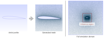
In order to generate ground truth data for training, we compute the velocity and pressure distributions of flows around airfoils. We consider a space of solutions with a range of Reynolds numbers million, incompressible flow, and angles of attack in the range of degrees. We obtained 1505 different airfoil shapes from the UIUC database [SoIaUCAD96], which were used to generate input data in conjunction with randomly sampled freestream conditions from the range described above. The RANS simulations make use of the widely used SA [SA92] one equation turbulence model, and solutions are calculated with the open source code OpenFOAM. Here we employ a body-fitted triangle mesh, with refinement near the airfoil. At the airfoil surface, the triangle mesh has an average edge length of to resolve the boundary layer of the flow. The discretization is coarsened to an edge length of near the domain boundary, which has an overall size of units. The airfoil has a length of unit. Typical examples from the training data set are shown in Fig. 2.
While typical RANS solvers, such as the one from OpenFOAM, require large distances for the domain boundaries in order to reduce their negative impact on the solutions around the airfoil, we can focus on a smaller region of units around the airfoil for the deep learning task. As our model directly learns from reference data sets that were generated with a large domain boundary distance, we do not need to reproduce solution in the whole space where the solution was computed, but rather can focus on the region in the vicinity of the airfoil without impairing the solution.
To facilitate NN architectures with convolutional layers, we resample this region with a Cartesian grid to obtain the ground truth pressure and velocity data sets, as shown in Fig. 3. The re-sampling is performed with a linear weighted interpolation of cell-centered values with a spacing of units in OpenFOAM. As for the domain boundaries, we only need to ensure that the original solution was produced with a sufficient resolution to resolve the boundary layer. As the solution is smooth, we can later on sample it with a reduced resolution. Both properties, the reduced spatial extent of the deep learning region and the relaxed requirements for the discretization, highlight advantages of deep learning methods over traditional solvers in our setting.
We randomly choose an airfoil, Reynolds number and angle of attack from the parameter ranges described above and compute the corresponding RANS solution to obtain data sets for the learning task. This set of samples is split into two parts: a larger fraction that is used for training, and a remainder that is only used for evaluating the current state of a model (the validation set). Details of the respective data set sizes are given in the appendix, we typically use an 80% to 20% split for training and validation sets, respectively. The validation set allows for an unbiased evaluation of the quality of the trained model during training, e.g., to detect overfitting.
To later on evaluate the capabilities of the trained models with respect to generalization, we use an additional set of 30 airfoil shapes that were not used for training, to generate a test data set with 90 samples (using the same range of Reynolds numbers and angles of attack as described above).
Pre-processing
As the resulting solutions of the RANS simulations have a size of , we use CNN architectures with inputs of the same size. The solutions globally depend on all boundary conditions. Accordingly, the architecture of the network makes sure this information is readily available spatially and throughout the different layers.
Thus freestream conditions and the airfoil shape are encoded in a grid of values. As knowledge about the targeted Reynolds number is required to compute the desired output, we encode the Reynolds number in terms of differently scaled freestream velocity vectors. I.e., for the smallest Reynolds numbers the freestream velocity has a magnitude of 0.1, while the largest ones are indicated by a magnitude of 1. The first of the three input channels contains a mask for the airfoil shape, 0 being outside, and 1 inside. The next two channels of the input contain x and y velocity components, respectively. Both velocity channels are initialized to the x and y component of the freestream conditions, respectively, with a zero velocity inside of the airfoil shape. Note that the inputs contain highly redundant information, they are essentially constant, and we likewise, redundantly, encode the airfoil shape in all three input fields.
The output data sets for supervised training have the same size of . Here, the first channel contains pressure , while the next two channels contain x and y velocity of the RANS solution, .
While the simulation data could be used for training in this form, we describe two further data pre-processing steps that we will evaluate in terms of their influence on the learned performance below. First, we can follow common practice and normalize all involved quantities with respect to the magnitude of the freestream velocity, i.e., make them dimensionless. Thus we consider , and . Especially the latter is important to remove the quadratic scaling of the pressure values from the target data. This flattens the space of solutions, and simplifies the task for the neural network later on.
In addition, only the pressure gradient is typically needed to compute the RANS solutions. Thus, as a second pre-processing variant we can additionally remove the mean pressure from each solution and define , with the pressure mean , where denotes the number of individual pressure samples . Without this removal of the mean values, the pressure targets represent an ill-posed learning goal as the random pressure offsets in the solutions are not correlated with the inputs.
As a last step, irrespective of which pre-processing method was used, each channel is normalized to the range in order to minimize errors from limited numerical precision during the training phase. We use the maximum absolute value for each quantity computed over the entire training data set to normalize the data. Both boundary condition inputs and ground truth solutions, i.e. output targets, are normalized in the same way. Note that the velocity is not offset, but only scaled by a global per component factor, even when using .
Neural Network Architecture
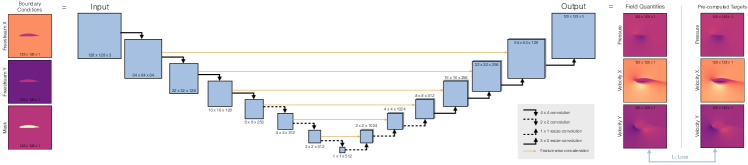
Our neural network model is based on the U-Net architecture [RFB15], which is widely used for tasks such as image translation. The network has the typical bowtie structure, translating spatial information into extracted features with convolutional layers. In addition, skip-connections from in- to output feature channels are introduced to ensure this information is available in the outputs layers for inferring the solution. We have experimented with a variety of architectures with different amounts of skip connections [BKC15, CC17, HLW16], and found that the U-net yields a very good quality with relatively low memory requirements. Hence, we will focus on the most successful variant, a modified U-net architecture in the following.
This U-Net is a special case of an encoder-decoder architecture. In the encoding part, the image size is progressively down-sampled by a factor of 2 with strided convolutions. The allows the network to extract increasingly large-scale and abstract information in the growing number of feature channels. The decoding part of the network mirrors this behavior, and increases the spatial resolution with average-depooling layers, and reduces the number of feature layers. The skip connections concatenate all channels from the encoding branch to the corresponding branch of the decoding part, effectively doubling the number of channels for each decoding block. These skip connections help the network to consider low-level input information during the reconstruction of the solution in the decoding layers. Each section of the network consists of a convolutional layer, a batch normalization layer, in addition to a non-linear activation function. For our standard U-net with 7.7m weights, we use 7 convolutional blocks to turn the input into a single data point with 512 features, typically using convolutional kernels of size (only the inner three layers of the encoder use kernels, see Appendix Architecture and Training Details). As activation functions we use leaky ReLU functions with a slope of 0.2 in the encoding layers, and regular ReLU activations in the decoding layers. The decoder part uses another 7 symmetric layers to reconstruct the target function with the desired dimensionality of .
While it seems wasteful to repeat the freestream conditions almost times, i.e., over the whole domain outside of the airfoil, this setup is very beneficial for the NN. We know that the solution everywhere depends on the boundary conditions, and while the network would eventually learn this and propagate the necessary information via the convolutional bowtie structure, it is beneficial for the training process to make sure this information is available everywhere right from the start. This motivates the architecture with redundant boundary condition information and skip connections.
Supervised Training
We train our architecture with the Adam optimizer [KB14], using 80k iterations unless otherwise noted. Our implementation is based on the PyTorch111From https://pytorch.org. deep learning framework. Due to the strictly supervised setting of our learning setup, we use a simple L1 loss , with being the output of the CNN. Here, an L2 loss could likewise be used and yields very similar results, but we found that L1 yields slight improvements. In both cases, a supervision for all cells of the inferred outputs in terms of a direct vector norm is important for stable training runs. The number of iterations was chosen such that the training runs converge to their final inference accuracies across all changes of hyperparameters and network architectures. Hence, to ensure that the different training runs below can be compared, we train all networks with the same number of training iterations.
Due to the potentially large number of local minima and the stochasticity of the training process, individual runs can yield significantly different results due to effects such as non-deterministic GPU calculations and/or different random seeds. While runs can be made deterministic, slight changes of the training data or their order can lead to similar differences in the trained models. Thus, in the following we present network performances across multiple training runs. For practical applications, a single, best performing model could be selected from such a collection of runs via cross validation. The following graphs, e.g. Fig. 5 and Fig. 6, show the mean and standard error of the mean for five runs, all with otherwise identical settings apart from different random seeds. Hence, the standard errors indicate the variance in result quality that can be expected for a selected training modality.
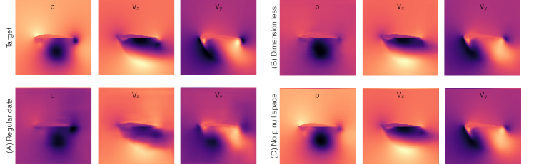
First, we illustrate the importance of proper data normalization. As outlined above we can train models either (A) with the pressure and velocity data exactly as they arise in the model equations, i.e., , or (B) we can normalize the data by velocity magnitude . Lastly, we can remove the pressure null space and train models with as target data (C). Not surprisingly, this makes a huge difference. For comparing the different variants, we de-normalize the data for (B) and (C), and then compute the averaged, absolute error w.r.t. ground truth pressure and velocity values for 400 randomly selected data sets. While variant (A) exhibits a very significant average error of , the data variant (B) has an average error of only , while (C) reduces this by another factor of ca. 4 to . An airfoil configuration that shows an example of how these errors manifest themselves in the inferred solutions can be found in Fig. 4.
Thus, in practice it is crucial to understand the data that the model should learn, and simplify the space of solutions as much as possible, e.g., by making use of the dimensionless quantities for fluid flow. Note that for the three models discussed above we have already used the training setup that we will explain in more detail in the following paragraphs. From now on, all models will only be trained with fully normalized data, i.e., case (C) above.
We have also experimented with adversarial training, and while others have noticed improvements [FGP17], we were not successful with GANs during our tests. While individual runs yielded good results, this was usually caused by sub-optimal settings for the corresponding supervised training runs. In a controlled setting such as ours, where we can densely sample the parameter space, we found that generating more training data, rather than switching to a more costly adversarial training, is typically a preferred way to improve the results.
Basic Parameters
In order to establish a training methodology, we first evaluate several basic training parameters, namely learning rate, learning rate decay, and normalization of the input data. In the following we will evaluate these parameters for a standard network size with a training data set of medium size (details given in Appendix Training Data).
One of the most crucial parameters for deep learning is the learning rate of the optimizer. The learning rate scales the step size the optimizer takes to update the weights of a neural network based on a gradient computed from one mini-batch of data. As the energy landscapes spanned by typical deep neural networks are often non-linear functions with large numbers of minima and saddle-points, small learning rates are not necessarily ideal, as the optimization might get stuck in undesirable states, while overly large ones can easily prevent convergence. Fig. 5 illustrates this for our setting. The largest learning rate clearly overshoots and has trouble converging. In our case the range of to yields good convergence.
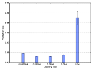
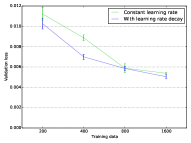
In addition, we found that learning rate decay, i.e., decreasing the learning rate during training, helps to stabilize the results, and reduce variance in performance. While the influence is not huge when the other parameters are chosen well, we decrease the learning rate to 10% of its initial value over the course of the second half of the training iterations. A comparison of four different settings each with and without learning rate decay is shown on the right of Fig. 5.
To prevent overfitting, i.e., the reproduction of single input-output pairs rather than a smooth reproduction of the function that should be approximated by the model, regularization is an important topic for deep learning methods. The most common regularization techniques are dropout, data augmentation, and early stopping [GBC16]. In addition, the loss function can be modified, typically with additional terms that minimize parts of the outputs or even the NN weights (weight decay) in terms of L1 or L2 norms. While this regularization is especially important for fully connected neural networks [LKT16, SMD17], we focus on CNNs in our study, which are inherently less prone to overfitting as they are applied to all spatial locations of an input, and typically receive a large variety of data configurations even from a single input to the NN.
In addition to the techniques outlined above, overfitting can also be avoided by ensuring that enough training data is available. While this is not always possible or practical, a key advantage of machine learning in the context of PDEs is that reliable training data can be generated in large amounts given enough computational resources. We will investigate the influence of varying amounts of training data for our models in more detail below. While we found a very slight amount of dropout to be preferable (see Section Architecture and Training Details), we will not use any other regularization methods. We found that our networks converged to stable levels in terms of training and validation losses, and hence do not employ early stopping in order to ensure all networks below were trained with the same number of iterations. It is also worth noting that data augmentation is difficult in our context, as each solution is unique for a given input configuration. Below, we instead focus on the influence of varying amounts of pre-computed training data on the generalizing capabilities of a trained network.
Note that due to the complexity of typical learning tasks for NNs it is non-trivial to find the best parameters for training. Typically, it would be ideal to perform broad hyperparameter searches for each of the different hyperparameters to evaluate their effect on inference accuracy. However, as differences of these searches were found to be relatively small in our case, the training parameters will be kept constant: the following training runs use a learning rate of 0.0004, a batch size of 10, and learning rate decay.
Accuracy
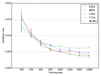
Having established a stable training setup, we can now investigate the accuracy of our network in more detail. Based on a database of 26.722 target solutions generated as described above, we have measured how the amount of available training data influences accuracy for validation data as well as generalization accuracy for a test data set. In addition, we measure how accuracy scales with the number of weights, i.e., degrees of freedom in the NN.
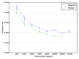
For the following training runs, the amount of training data is scaled from 100 samples to 12800 samples in factors of two, and we vary the number of weights by scaling the number of feature maps in the convolutional layers of our network. As the size of the kernel tensor of a convolutional layer scales with the number of input channels times number of output channels, a 2x increase of channels leads to a roughly four-fold increase in overall weights (biases change linearly). The corresponding accuracy graphs for five different network sizes can be seen in Fig. 6. As outlined above, five models with different random seeds (and correspondingly different sets of training data) where trained for each of the data points, standard errors are shown with error bars in the graphs. The different networks have 122.979, 487.107, 1.938.819, 7.736.067, and 30.905.859 weights, respectively. The validation loss in Fig. 6,top shows how the models with little amounts of training data exhibit larger errors, and vary very significantly in terms of performance. The behavior stabilizes with larger amounts of data being available for training, and the models saturate in terms of inference accuracy at different levels that correspond to their weight numbers. Comparing the curves for the 122k and 30.9m models, the former exhibits a flatter curve with lower errors in the beginning (due to inherent regularization from the smaller number of weights), and larger errors at the end. The 30.9m instead more strongly overfits to the data initially, and yields a better performance when enough data is available. In this case the mean error for the latter model is 0.0033 compared to 0.0063 for the 122k model.
The graphs also show how the different models start to saturate in terms of loss reduction once a certain amount of training data is available. For the smaller models this starts to show around 1000 samples, while the trends of the larger models indicate that they could benefit from even more training data. The loss curves indicate that despite the 4x increase in weights for the different networks, roughly doubling the amount of training data is sufficient to reach a similar saturation point.
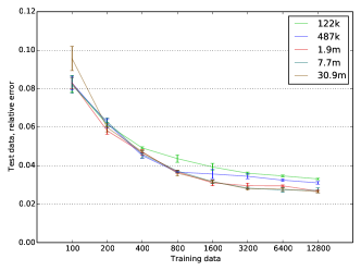
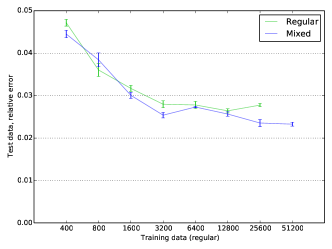
The bottom graph of Fig. 6 shows the performance of the different models for a test set of 30 airfoils that were not seen during training. Freestream velocities were randomly sampled from the same distribution used for training data generation (see Section 4) to produce 90 test data sets. We use this data to measure how well the trained models can generalize to new airfoil shapes. Instead of the L1 loss that was used for the validation data, this graph shows the mean relative error of the normalized quantities (the L1 loss behavior is line with the relative errors shown here). The relative error is computed with , with being the number of samples, in our case, the function under consideration, e.g., pressure, and the approximation of the neural network. We found the average relative error for all inferred fields, i.e. to be a good metric to evaluate the models, as it takes all outputs into account and directly yields an error percentage for the accuracy of the inferred solutions. In addition, it sheds light on the relative accuracy of the inferred solutions, while the L1 metric yields estimates of the averaged differences. Hence, both metrics are important for evaluating the overall accuracy of the trained models.
For this test set, the curves exhibit a similar fall-off with reduced errors for larger amounts of training data, but the difference between the different model sizes is significantly smaller. With the largest amount of training data (12.8k samples), the difference in test error between smallest and largest models is 0.033 versus 0.026. Thus, the latter network achieves an average relative error of 2.6% across all three output channels. Due to the differences between velocity and pressure functions, this error is not evenly distributed. Rather, the model is trained for reducing differences across all three output quantities, which yields relative errors of 2.15% for the x velocity channel, 2.6% for y, and 14.76% for pressure values. Especially the relatively large amount of small pressure values with fewer large spikes in the harmonic functions lead to increased relative errors for the pressure channel. If necessary, this could be alleviated by changing the loss function, but as the goal of this study is to consider generic CNN performance, we will continue to use loss in the following.
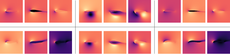
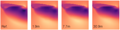
Also, it is visible in Fig. 6 that the three largest model sizes yield a very similar performance. While the models improve in terms of capturing the space of training data, as visible from the validation loss at the top of Fig. 6, this does not directly translate into an improved generalization. The additional training data in this case does not yield new information for the unseen shapes. An example data set with inferred solutions is visualized in Fig. 7. Note that the relatively small numeric changes of the overall test error lead to significant differences in the solutions.
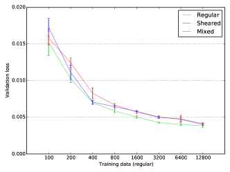
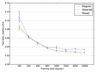
To investigate the generalization behavior in more detail, we have prepared an augmented data set, where we have sheared the airfoil shapes by degrees along a centered x-axis to enlarge the space of shapes seen by the networks. The corresponding relative error graphs for a model with 7.7m weights are shown in Fig. 10. Here we compare three variants, a model trained only with regular data (this is identical to Fig. 6), models purely trained with the sheared data set, and a set of models trained with 50% of the regular data, and 50% of the sheared data. We will refer to these data sets as regular, sheared, and mixed in the following. It is apparent that both the sheared and mixed data sets yield a larger validation error for large training data amounts (Fig. 10, top). This is not surprising, as the introduction of the sheared data leads to an enlarged space of solutions, and hence also a more difficult learning task. Fig. 10 bottom shows that despite this enlarged space, the trained models do not perform better on the same test data set from above. Rather, the performance decreases when only using the sheared data (blue line in Fig. 10, bottom).
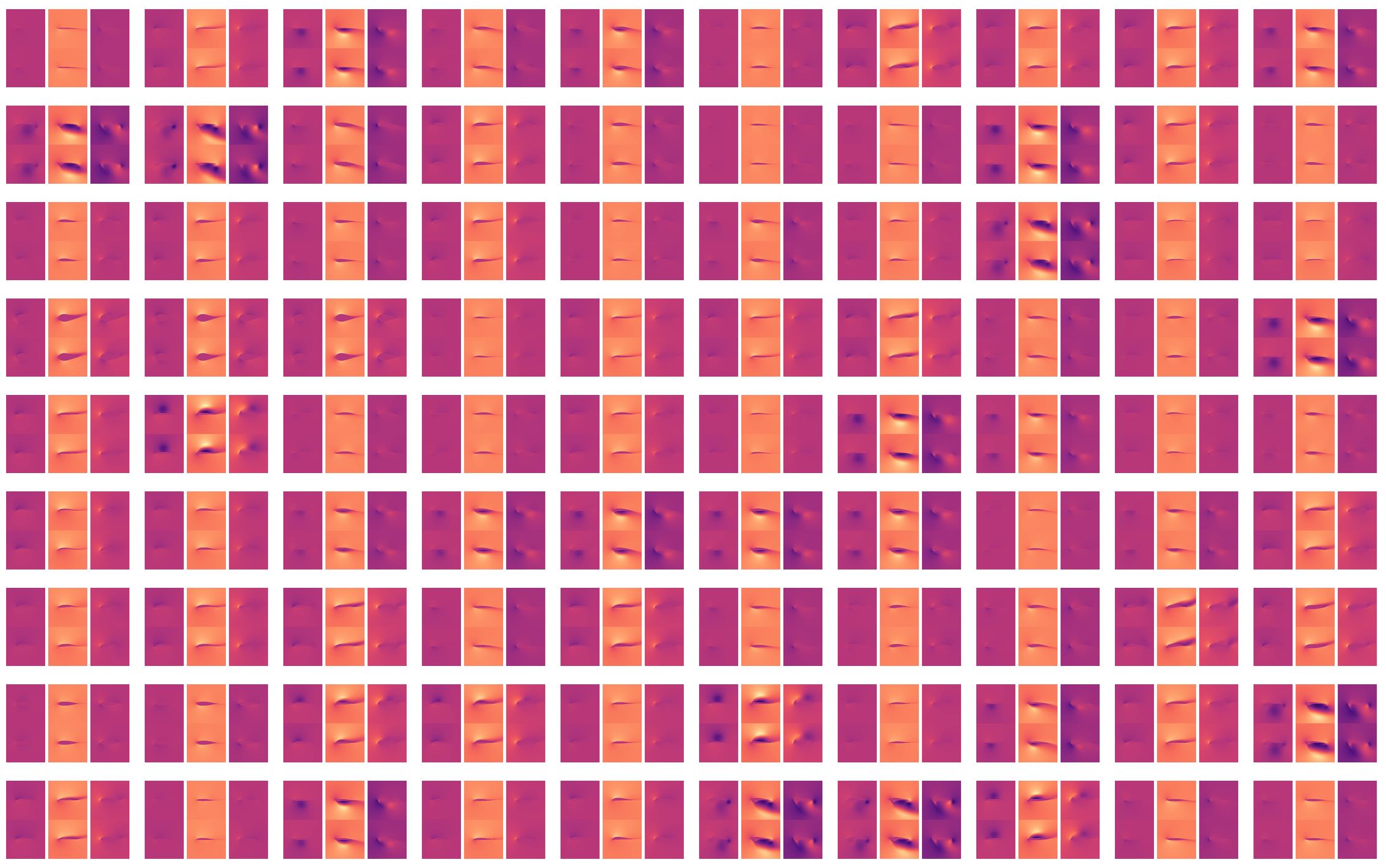
This picture changes when using a larger model. Training the 30.9m weight model with the mixed data set leads to improvements in performance when there is enough data, especially for the run with 25600 training samples in Fig. 11. In this case, the large model outperforms the regular data model with an average relative error of 2.77%, and yields an error of 2.35%. Training the 30.9m model with 51k of mixed samples slightly improves the performance to 2.32%. Hence, the generalization performance not only depends on type and amount of training data, but also on the representative capacities of the chosen CNN architecture. The full set of test data outputs for this model is shown in Fig. 14.
Performance
The central motivation for deep learning in the context of physics simulations is arguably performance. In our case, evaluating the trained 30.9m model for a single data point on an NVidia GTX 1080 GPU takes 5.53ms (including data transfer to the GPU). This runtime, like all following ones, is averaged over multiple runs. The network evaluation itself, i.e. without GPU overhead, takes 2.10ms. The runtime per solution can be reduced significantly when evaluating multiple solutions at once, e.g., for a batch size of 8, the evaluation time rises only slightly to 2.15ms. In contrast, computing the solution with OpenFOAM requires 40.4s when accuracy is adjusted to match the network outputs. The runs for training data generation took 71.9s.
While it is of course problematic to compare implementations as different as the two at hand, it still yields a realistic baseline of the performance we can expect from publicly available open source solvers. OpenFOAM clearly leaves significant room for performance, e.g., its solver is currently single-threaded. This likewise holds on the deep learning side: The fast execution time of the discussed architectures can be achieved ”out-of-the-box” with PyTorch, and based on future hardware developments such as GPUs with built-in support for NN evaluation, we expect this performance to improve significantly even without any changes to the trained model itself. Thus, based on the current state of OpenFOAM and PyTorch, our models yield a speed up factor of ca. 1000.
The timings of training runs for the models discussed above vary with respect to the amount of data and model size, but start with 26 minutes for the 122k models, up to 147 min. for the 30.9m models.
Discussion
Overall, our best models yield a very good accuracy of less than 3% relative error. However, it is naturally an important question how this error can be further reduced. Based on our tests, this will require substantially larger training data sets and CNN models. It also becomes apparent from Fig. 6 that simply increasing model and training data size will not scale to arbitrary accuracies. Rather, this points towards the need to investigate and develop different approaches and network architectures.
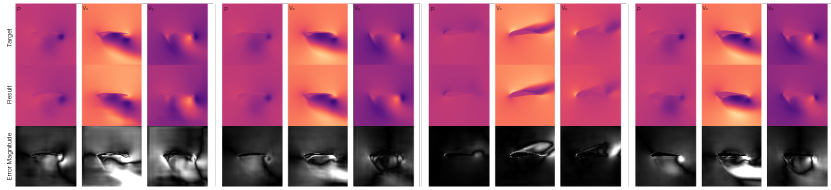
In addition, it is interesting to investigate how systematic the model errors are. Fig. 8 shows a selection of inferred results from the 7.7m model trained with 12k data sets. All results are taken from the test data set. As can be seen in the error magnitude visualizations in the bottom row of Fig. 8, the model is not completely off for any of the cases. Rather, errors typically manifest themselves as shifts in the inferred shapes of the wakes behind the airfoil. We also noticed that while they change w.r.t. details in the solution, the error typically remains large for most of the difficult cases of the test data set throughout the different runs. Most likely, this is caused by a lack of new information the models can extract from the training data sets that were used in the study. Here, it would also be interesting to consider an even larger test data set to investigate generalization in more detail.
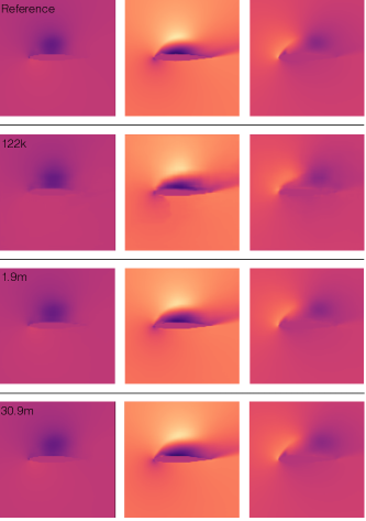
Finally, it is worth pointing out that despite the stagnated error measurements of the larger models in Fig. 6, the results consistently improve, especially regarding their sharpness. This is illustrated with a zoom in on a representative case for x velocity in Fig. 9, and we have noticed this behavior across the board for all channels and many data sets. As can be seen there, the sharpness of the inferred function increases, especially when comparing the 1.9m and 30.9m models, which exhibit the same performance in Fig. 6. This behavior can be partially attributed to these improvements being small in terms of scale. However, as it is noticeable consistently, it also points to inherent limitations of direct vector norms as loss functions.
5 Conclusions
We have presented a first study of the accuracy of deep learning for the inference of RANS solutions for airfoils. While the results of our study are by no means guaranteed to directly carry over to other problems due to the inherent differences of solution spaces for different physical problems, we believe that our results can nonetheless serve as a good starting point with respect to general methodology, data handling, and training procedures. We hope that they will provide a starting point for researchers, and help to overcome skepticism from a perceived lack of theoretical results. Flow simulations are a good example of a field that has made tremendous steps forward despite unanswered questions regarding theory: although it is unknown whether a finite time singularity for the Navier-Stokes equations exists, this luckily has not stopped research in the field. Likewise, we believe there is huge potential for deep learning in the CFD context despite the open questions regarding theory.
In addition we have outlined a simulation and training setup that is on the one hand relatively simple, but nonetheless offers a large amount of complexity for machine learning algorithms. It also illustrates that a physical understanding of the problem is crucial, as the nondimensional formulation of the problem leads to significantly improved results without any changes to the deep learning components themselves. I.e., it is important to formulate the problem such that the relationship between input and output quantities is as simple as possible. The proposed setting provides a good point of entry for CFD researchers to experiment with deep learning algorithms, as well as a benchmark case for the evaluation of novel learning methods for fluids and related physics problems.
We see numerous avenues for future work in the area of physics-based deep learning, e.g., to employ trained flow models in the context of inverse problems. The high performance and differentiability of a CNN model yields a very good basis for tough problems such as flow control and shape optimization.
Appendix
Architecture and Training Details
The network is fully convolutional with 14 layers, and consists of a series of convolutional blocks. All blocks have a similar structure: activation, convolution, batch normalization and dropout. Instead of transpose convolutions with strides, we use a linear upsampling ”up()” followed by a convolution on the upsampled content [ODO16]. In addition, the kernel size is reduced by one in the decoder part to ensure uneven kernel sizes, i.e., convolutions with symmetric kernels.
Convolutional blocks below are parametrized by an output channel factor , kernel size , stride , where we use as short form for . Note that the input channels for the decoder part have twice the size due to the concatenation of features from the encoder part (this is not explicitly written out in our notation). Batch normalization is indicated by below. Activation by ReLU is indicated by , while indicates a leaky ReLU [MHN13, RMC16] with a slope of . Slight dropout with a rate of 0.01 is used for all layers. The different models above use a channel base multiplier that is multiplied by for the individual layers. was and for the 122k, 487k, 1.9m, 7.7m and 30.9m models discussed above. Thus, e.g., for a block with has channels. Channel wise concatenation is denoted by ”conc()”. Addendum: Note that below inadvertently used a kernel size of 2 in our original implementation, and is listed as such here. While for symmetry with the decoder part, would be preferable here, this should not lead to substantial changes in terms of inference results.
The network receives an input with three channels (as outlined in Section 4) and can be summarized as:
Here represents the output of the network, and the corresponding convolution generates 3 output channels. Unless otherwise noted, training runs are performed with iterations of the Adam optimizer using and , learning rate with learning rate decay and batch size . Fig. 5 used a model with 7.7m weights, iterations, and 8k training data samples, 75% regular, and 25% sheared. Fig. 4 used a model with 7.7m weights, with 12.8k training data samples, 75% regular, and 25% sheared.
Training Data
In the following, we also give details of the different training data set sizes used in the training runs above. We start with a minimal size of 100 samples, and increase the data set size in factors of two up to 12800. Typically, the total number of samples is split into 80% training data, and 20% validation data. However, we found validation sets of several hundred samples to yield stable estimates. Hence, we use an upper limit of 400 as the maximal size of the validation data set. The corresponding number of samples are randomly drawn from a pool of 26732 pre-computed pairs of boundary conditions and flow solutions computed with OpenFOAM. The exact sizes used for the training runs of Fig. 5 and Fig. 6 are given in Table 1. The dimensionality of the different data sets is summarized in Table 2.
| Total dataset size | Training | Validation |
|---|---|---|
| 100 | 80 | 20 |
| 200 | 160 | 40 |
| 400 | 320 | 80 |
| 800 | 640 | 160 |
| 1600 | 1280 | 320 |
| 3200 | 2800 | 400 |
| 6400 | 6000 | 400 |
| 12800 | 12400 | 400 |
| 25600 | 25200 | 400 |
| Quantity | Dimension |
|---|---|
| Airfoil shapes (training, validation) | 1505 |
| Airfoil shapes (test) | 30 |
| RANS solutions (regular) | 26732 |
| RANS solutions (sheared) | 27108 |
In addition to this regular data set, we employ a sheared data set that contains sheared airfoil profiles (as described above). This data set has an overall size of 27108 samples, and was used for the sheared models in Fig. 10 with the same training set sizes as shown in Table 1. We also trained models with a mixed data set, shown in Fig. 10 and Fig. 11 that contains half regular, and half sheared samples. I.e., the five models for in Fig. 11 employed 320 samples drawn from the regular plus 320 drawn from the sheared data set for training, and 80 regular plus 80 sheared samples for validation. For the mixed data set, we additionally train a large model with a total dataset size of 25600, i.e., the bottom line of Fig. 1, that is shown in Fig. 11.
Training Evolution and Dropout
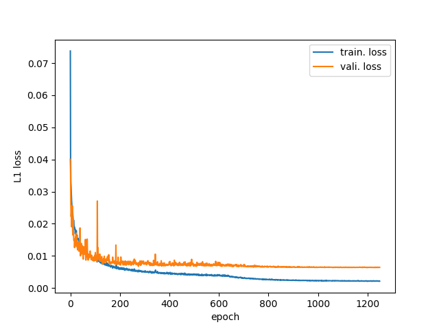
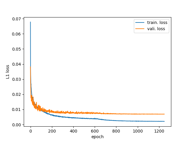
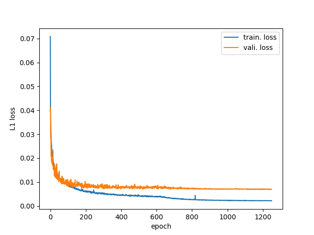
In Fig. 12 we show three examples of training runs of typical model used on the accuracy evaluations above. These graphs show that the models converge to stable levels of training and validation loss, and do not exhibit overfitting over time. Additionally, the onset of learning rate decay can be seen in the middle of the graph. This noticeably reduces the variance of the learning iterations, and let’s the training process fine-tune the current state of the model.
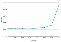
Fig. 13 evaluates the effect of varying dropout rates. Different amounts of dropout applied at training time are shown along x with the resulting test accuracies. It becomes apparent that the effect is relatively small, but overall the accuracy deteriorates with increasing amounts of dropout.
Funding Sources
This work is supported by ERC Starting Grant 637014 (realFlow) and the TUM PREP internship program.
Acknowledgments
We thank H. Mehrotra, and N. Mainali for their help with the deep learning experiments, and the anonymous reviewers for the helpful comments to improve our work.
References
- [ADMG17] Panos Achlioptas, Olga Diamanti, Ioannis Mitliagkas, and Leonidas Guibas. Representation learning and adversarial generation of 3d point clouds. arXiv preprint arXiv:1707.02392, 2017.
- [BFM18] Andrea Beck, David Flad, and Claus-Dieter Munz. Deep neural networks for data-driven turbulence models. ResearchGate preprint, 2018.
- [Bis06] Christopher M. Bishop. Pattern Recognition and Machine Learning (Information Science and Statistics). Springer-Verlag New York, Inc., Secaucus, NJ, USA, 2006.
- [BKC15] Vijay Badrinarayanan, Alex Kendall, and Roberto Cipolla. Segnet: A deep convolutional encoder-decoder architecture for image segmentation. arXiv preprint, abs/1511.00561, 2015.
- [BOCPZ12] Alfonso Bueno-Orovio, Carlos Castro, Francisco Palacios, and Enrique Zuazua. Continuous adjoint approach for the spalart-allmaras model in aerodynamic optimization. AIAA journal, 50(3):631–646, 2012.
- [BPL+16] Peter Battaglia, Razvan Pascanu, Matthew Lai, Danilo Jimenez Rezende, et al. Interaction networks for learning about objects, relations and physics. In Advances in Neural Information Processing Systems, pages 4502–4510, 2016.
- [BRFF18] Pierre Baqué, Edoardo Remelli, François Fleuret, and Pascal Fua. Geodesic convolutional shape optimization. arXiv preprint arXiv:1802.04016, 2018.
- [BSHHB18] Yohai Bar-Sinai, Stephan Hoyer, Jason Hickey, and Michael P Brenner. Data-driven discretization: a method for systematic coarse graining of partial differential equations. arXiv preprint arXiv:1808.04930, 2018.
- [CC17] Abhishek Chaurasia and Eugenio Culurciello. Linknet: Exploiting encoder representations for efficient semantic segmentation. arXiv preprint, abs/1707.03718, 2017.
- [CT17] Mengyu Chu and Nils Thuerey. Data-driven synthesis of smoke flows with CNN-based feature descriptors. ACM Trans. Graph., 36(4)(69), 2017.
- [CUTT16] Michael B Chang, Tomer Ullman, Antonio Torralba, and Joshua B Tenenbaum. A compositional object-based approach to learning physical dynamics. arXiv:1612.00341, 2016.
- [Dur18] Paul A Durbin. Some recent developments in turbulence closure modeling. Annual Review of Fluid Mechanics, 50:77–103, 2018.
- [ECDB14] WN Edeling, Pasquale Cinnella, Richard P Dwight, and Hester Bijl. Bayesian estimates of parameter variability in the k– turbulence model. Journal of Computational Physics, 258:73–94, 2014.
- [EMMV17] Sebastien Ehrhardt, Aron Monszpart, Niloy J Mitra, and Andrea Vedaldi. Learning a physical long-term predictor. arXiv:1703.00247, 2017.
- [FGP17] Amir Barati Farimani, Joseph Gomes, and Vijay S Pande. Deep learning the physics of transport phenomena. arXiv preprint arXiv:1709.02432, 2017.
- [FVT08] Jochen Fröhlich and Dominic Von Terzi. Hybrid les/rans methods for the simulation of turbulent flows. Progress in Aerospace Sciences, 44(5):349–377, 2008.
- [GBC16] Ian Goodfellow, Yoshua Bengio, and Aaron Courville. Deep Learning. MIT Press, 2016.
- [GPAM+14] Ian J Goodfellow, Jean Pouget-Abadie, Mehdi Mirza, Bing Xu, David Warde-Farley, Sherjil Ozair, Aaron Courville, and Yoshua Bengio. Generative adversarial nets. stat, 1050:10, 2014.
- [GR99] Roxana M Greenman and Karlin R Roth. High-lift optimization design using neural networks on a multi-element airfoil. Journal of fluids engineering, 121(2):434–440, 1999.
- [GSV04] Georges A Gerolymos, Emilie Sauret, and I Vallet. Contribution to single-point closure reynolds-stress modelling of inhomogeneous flow. Theoretical and Computational Fluid Dynamics, 17(5-6):407–431, 2004.
- [HLW16] Gao Huang, Zhuang Liu, and Kilian Q. Weinberger. Densely connected convolutional networks. arXiv preprint, abs/1608.06993, 2016.
- [IZZE16] Phillip Isola, Jun-Yan Zhu, Tinghui Zhou, and Alexei A. Efros. Image-to-image translation with conditional adversarial networks. CoRR, abs/1611.07004, 2016.
- [IZZE17] Phillip Isola, Jun-Yan Zhu, Tinghui Zhou, and Alexei A Efros. Image-to-image translation with conditional adversarial networks. Proc. of IEEE Comp. Vision and Pattern Rec., 2017.
- [JGSC15] Zhaoyin Jia, Andrew C Gallagher, Ashutosh Saxena, and Tsuhan Chen. 3d reasoning from blocks to stability. IEEE transactions on pattern analysis and machine intelligence, 37(5):905–918, 2015.
- [KALL17] Tero Karras, Timo Aila, Samuli Laine, and Jaakko Lehtinen. Progressive growing of gans for improved quality, stability, and variation. arXiv:1710.10196, 2017.
- [KAT+18] Byungsoo Kim, Vinicius C Azevedo, Nils Thuerey, Theodore Kim, Markus Gross, and Barbara Solenthaler. Deep fluids: A generative network for parameterized fluid simulations. arXiv preprint arXiv:1806.02071, 2018.
- [KB14] Diederik Kingma and Jimmy Ba. Adam: A method for stochastic optimization. arXiv:1412.6980, 2014.
- [KD98] Doyle D Knight and Gerard Degrez. Shock wave boundary layer interactions in high mach number flows a critical survey of current numerical prediction capabilities. AGARD ADVISORY REPORT AGARD AR, 2:1–1, 1998.
- [KSH12] Alex Krizhevsky, Ilya Sutskever, and Geoffrey E Hinton. Imagenet classification with deep convolutional neural networks. In Advances in Neural Information Processing Systems, pages 1097–1105. NIPS, 2012.
- [LKT16] Julia Ling, Andrew Kurzawski, and Jeremy Templeton. Reynolds averaged turbulence modelling using deep neural networks with embedded invariance. Journal of Fluid Mechanics, 807:155–166, 2016.
- [LT15] Julia Ling and J Templeton. Evaluation of machine learning algorithms for prediction of regions of high reynolds averaged navier stokes uncertainty. Physics of Fluids, 27(8):085103, 2015.
- [LTH+16] Christian Ledig, Lucas Theis, Ferenc Huszár, Jose Caballero, Andrew Cunningham, Alejandro Acosta, Andrew Aitken, Alykhan Tejani, Johannes Totz, Zehan Wang, et al. Photo-realistic single image super-resolution using a generative adversarial network. arXiv:1609.04802, 2016.
- [MDB17] Lukas Mosser, Olivier Dubrule, and Martin J Blunt. Reconstruction of three-dimensional porous media using generative adversarial neural networks. arXiv:1704.03225, 2017.
- [MHN13] Andrew L. Maas, Awni Y. Hannun, and Andrew Y. Ng. Rectifier nonlinearities improve neural network acoustic models. In Proc. ICML, volume 30(1), 2013.
- [MO14] Mehdi Mirza and Simon Osindero. Conditional generative adversarial nets. arXiv preprint arXiv:1411.1784, 2014.
- [ODO16] Augustus Odena, Vincent Dumoulin, and Chris Olah. Deconvolution and checkerboard artifacts. Distill, 2016.
- [PBT19] Lukas Prantl, Boris Bonev, and Nils Thuerey. Generating liquid simulations with deformation-aware neural networks. ICLR, 2019.
- [PM14] Svetlana Poroseva and Scott M Murman. Velocity/pressure-gradient correlations in a FORANS approach to turbulence modeling. In 44th AIAA Fluid Dynamics Conference, page 2207, 2014.
- [RBST03] T Rung, U Bunge, M Schatz, and F Thiele. Restatement of the spalart-allmaras eddy-viscosity model in strain-adaptive formulation. AIAA journal, 41(7):1396–1399, 2003.
- [RDL+18] Jaideep Ray, Lawrence Dechant, Sophia Lefantzi, Julia Ling, and Srinivasan Arunajatesan. Robust bayesian calibration of ak- model for compressible jet-in-crossflow simulations. AIAA Journal, 56(12):4893–4909, 2018.
- [RFB15] Olaf Ronneberger, Philipp Fischer, and Thomas Brox. U-net: Convolutional networks for biomedical image segmentation. In International Conference on Medical Image Computing and Computer-Assisted Intervention, pages 234–241. Springer, 2015.
- [RMC16] Alec Radford, Luke Metz, and Soumith Chintala. Unsupervised representation learning with deep convolutional generative adversarial networks. Proc. ICLR, 2016.
- [RYK18] Maziar Raissi, Alireza Yazdani, and George Em Karniadakis. Hidden fluid mechanics: A navier-stokes informed deep learning framework for assimilating flow visualization data. arXiv preprint arXiv:1808.04327, 2018.
- [SA92] P. Spalart and S. Allmaras. A one-equation turbulence model for aerodynamic flows. In 30th aerospace sciences meeting and exhibit, page 439, 1992.
- [SGS+18] Christian Soize, Roger Ghanem, Cosmin Safta, Xun Huan, Zachary P Vane, Joseph C Oefelein, Guilhem Lacaze, and Habib N Najm. Enhancing model predictability for a scramjet using probabilistic learning on manifolds. AIAA Journal, 57(1):365–378, 2018.
- [SLHA13] John Schulman, Alex Lee, Jonathan Ho, and Pieter Abbeel. Tracking deformable objects with point clouds. In Robotics and Automation (ICRA), 2013 IEEE International Conference on, pages 1130–1137. IEEE, 2013.
- [SMD17] Anand Pratap Singh, Shivaji Medida, and Karthik Duraisamy. Machine-learning-augmented predictive modeling of turbulent separated flows over airfoils. AIAA Journal, pages 2215–2227, 2017.
- [SoIaUCAD96] M.S. Selig, University of Illinois at Urbana-Champaign. Aeronautical, and Astronautical Engineering Department. UIUC Airfoil Data Site. Department of Aeronautical and Astronautical Engineering University of Illinois at Urbana-Champaign, 1996.
- [SSST99] M Shur, PR Spalart, M Strelets, and A Travin. Detached-eddy simulation of an airfoil at high angle of attack. In Engineering Turbulence Modelling and Experiments 4, pages 669–678. Elsevier, 1999.
- [SZSK19] Vinothkumar Sekar, Mengqi Zhang, Chang Shu, and Boo Cheong Khoo. Inverse design of airfoil using a deep convolutional neural network. AIAA Journal, pages 1–11, 2019.
- [TDA13] Brendan Tracey, Karthik Duraisamy, and Juan Alonso. Application of supervised learning to quantify uncertainties in turbulence and combustion modeling. In 51st AIAA Aerospace Sciences Meeting including the New Horizons Forum and Aerospace Exposition, page 259, 2013.
- [TDA15] Brendan D Tracey, Karthikeyan Duraisamy, and Juan J Alonso. A machine learning strategy to assist turbulence model development. In 53rd AIAA Aerospace Sciences Meeting, page 1287, 2015.
- [TMM+18] N. Thuerey, H. Mehrotra, N. Mainali, K. Weissenow, L. Prantl, and Xiangyu Hu. Deep Flow Prediction. Technical University of Munich (TUM), 2018.
- [TSSP16] Jonathan Tompson, Kristofer Schlachter, Pablo Sprechmann, and Ken Perlin. Accelerating eulerian fluid simulation with convolutional networks. arXiv: 1607.03597, 2016.
- [UB18] Nobuyuki Umetani and Bernd Bickel. Learning three-dimensional flow for interactive aerodynamic design. ACM Trans. Graph., 37(4):89, 2018.
- [UHT17] Kiwon Um, Xiangyu Hu, and Nils Thuerey. Splash modeling with neural networks. arXiv:1704.04456, 2017.
- [WBT18] Steffen Wiewel, Moritz Becher, and Nils Thuerey. Latent-space physics: Towards learning the temporal evolution of fluid flow. arXiv:1801, 2018.
- [WL02] D Keith Walters and James H Leylek. A new model for boundary-layer transition using a single-point rans approach. In ASME 2002 International Mechanical Engineering Congress and Exposition, pages 67–79. American Society of Mechanical Engineers, 2002.
- [WZW+17] Nicholas Watters, Daniel Zoran, Theophane Weber, Peter Battaglia, Razvan Pascanu, and Andrea Tacchetti. Visual interaction networks. In Advances in Neural Information Processing Systems, pages 4540–4548, 2017.
- [XFCT18] You Xie, Erik Franz, Mengyu Chu, and Nils Thuerey. tempogan: A temporally coherent, volumetric gan for super-resolution fluid flow. ACM Trans. Graph., 37(4), 2018.
- [YH18] Jian Yu and Jan S Hesthaven. Flowfield reconstruction method using artificial neural network. Aiaa Journal, 57(2):482–498, 2018.
- [YSJ18] Chulhee Yun, Suvrit Sra, and Ali Jadbabaie. A critical view of global optimality in deep learning. arXiv preprint arXiv:1802.03487, 2018.
- [YYX16] Cheng Yang, Xubo Yang, and Xiangyun Xiao. Data-driven projection method in fluid simulation. Computer Animation and Virtual Worlds, 27(3-4):415–424, 2016.
- [YZAY17] Rose Yu, Stephan Zheng, Anima Anandkumar, and Yisong Yue. Long-term forecasting using tensor-train rnns. arXiv preprint arXiv:1711.00073, 2017.
- [ZPIE17] Jun-Yan Zhu, Taesung Park, Phillip Isola, and Alexei A Efros. Unpaired image-to-image translation using cycle-consistent adversarial networks. arXiv:1703.10593, 2017.
- [ZSM17] Y. Zhang, W.-J. Sung, and D. Mavris. Application of Convolutional Neural Network to Predict Airfoil Lift Coefficient. arXiv preprint, December 2017.
- [ZZJ+14] Bo Zheng, Yibiao Zhao, C Yu Joey, Katsushi Ikeuchi, and Song-Chun Zhu. Detecting potential falling objects by inferring human action and natural disturbance. In Robotics and Automation (ICRA), 2014 IEEE International Conference on, pages 3417–3424. IEEE, 2014.