Universal $d=1$ flat band generator from compact localized states

Abstract

The band structure of some translationally invariant lattice Hamiltonians contains strictly dispersionless flat bands(FB). These are induced by destructive interference, and typically host compact localized eigenstates (CLS) which occupy a finite number $U$ of unit cells. FBs are important due to macroscopic degeneracy and consequently due to their high sensitivity and strong response to different types of weak perturbations. We use a recently introduced classification of FB networks based on CLS properties, and extend the FB Hamiltonian generator introduced in Phys. Rev. B 95, 115135 (2017) to an arbitrary number $\nu$ of bands in the band structure, and arbitrary size $U$ of a CLS. The FB Hamiltonian is a solution to equations that we identify with an inverse eigenvalue problem. These can be solved only numerically in general. By imposing additional constraints, e.g. a chiral symmetry, we are able to find analytical solutions to the inverse eigenvalue problem.

I Introduction

Physical models featuring macroscopically degenerate eigenstates have attracted a lot of attention in the past decades. Such degeneracies are naturally unstable to slightest perturbations making them perfect candidates for exotic or unconventional correlated phases of matter like in frustrated magnetism, and strongly correlated systems. An active field in this direction is the understanding of properties of flat bands (FB), i.e., bands with no dispersion Derzhko et al. (2015); Leykam et al. (2018). FB models are usually translationally invariant tight-binding networks which are characterized by a certain hopping connectivity between different network sites and which characterize the wave function of, e.g., a quantum particle, a macroscopic condensate, or a photonic field in a structured medium Leykam et al. (2018); Leykam and Flach (2018). The band structure of the corresponding eigenvalue problem contains $\nu$ bands if the unit cell of the network is containing $\nu$ sites. FB networks were widely studied theoretically in lattice dimension $d=1$ Derzhko and Richter (2006); Derzhko et al. (2010); Hyrkäs et al. (2013), $d=2$ Mielke (1991a); Tasaki (1992); Misumi and Aoki (2017), and in $d=3$ Mielke (1991a); Nishino and Goda (2005); Lieb (1989); Mielke (1991b, 1992); Brandt and Giesekus (1992); Ramachandran et al. (2017). FBs have been experimentally realized in a variety of setups, including optical wave guide networks, exciton-polariton condensates, and ultra-cold atomic condensates Guzmán-Silva et al. (2014); Vicencio et al. (2015); Mukherjee and Thomson (2015); Weimann et al. (2016); Xia et al. (2016); Taie et al. (2015); Jo et al. (2012); Masumoto et al. (2012); Baboux et al. (2016).

The absence of dispersion in FBs happens due to destructive interference. Destructive interference is also the cause of the existence of compact localized states (CLS). CLS are eigenstates at the FB energy, that have strictly finite support on the lattice, and occupy a finite number $U$ of unit cells. Since any translation of a CLS is necessarily again an eigenstate for a translationally invariant Hamiltonian, the existence of a CLS is a direct proof of existence of an FB and its macroscopic degeneracy.

System perturbations typically destroy CLS leading to a variety of interesting phenomena: flat-band ferromagnetism in the fermionic Hubbard model, Mielke (1991b, a); Tasaki (1992); Mielke and Tasaki (1993); Tasaki (2008, 1994); Maksymenko et al. (2012) energy dependent scaling of disorder-induced localization length Leykam et al. (2017a), singular mobility edges with quasiperiodic potentials Bodyfelt et al. (2014); Danieli et al. (2015), Landau-Zener Bloch oscillations in the presence of external fields Khomeriki and Flach (2016), discrete breathers in nonlinear flat band lattices, Danieli et al. (2018); Johansson et al. (2015); Real and Vicencio (2018), pair formation of hard core bosons Mielke (2018), and geometric origin of superfluidity Peotta and Törmä (2015); Julku et al. (2016). Several approaches were developed to construct FB networks: line graph constructions Mielke (1991a), decorated lattices Tasaki (1992), origami rules Dias and Gouveia (2015), repetition of mini-arrays Morales-Inostroza and Vicencio (2016), chiral symmetry based ones Ramachandran et al. (2017), and methods based on local symmetries of the Hamiltonian Röntgen et al. (2018). Nishino et al. Nishino et al. (2003); Nishino and Goda (2005) used specific CLS and network symmetries to fine-tune the hoppings down to a FB.

A systematic classification of FBs in terms of compact localized states was introduced in Ref. Flach et al., 2014 where FBs are classified by the size $U$ of the CLS: the number of unit cells occupied by CLS. CLS-based FB generators were then obtained for $U=1$ and arbitrary number of bands and dimension Flach et al. (2014) covering all FB models of that class. For $\nu=2$ and $U=2$ in one dimension, a generator was obtained in Ref. Maimaiti et al., 2017 describing all the possible $d=1$ FB networks with two bands. These FB networks form a two-parameter family of generalized sawtooth chains.

In this work we focus on the case $d=1$ deferring higher dimensions, where we expect even richer phenomenology, for future work. The $d=1$ case was so far analyzed only for two bands and $U=2$ Maimaiti et al. (2017). Many recent theoretical proposals Morales-Inostroza and Vicencio (2016); Mondaini et al. (2018); Gligorić et al. (2019); Tovmasyan et al. (2018, 2016, 2013); Longhi (2019); Vakulchyk et al. (2017) and experimental attempts of realizations Baboux et al. (2016); Travkin et al. (2017); Mukherjee and Thomson (2015); Weimann et al. (2016) focus on $d=1$ settings, and make it necessary to obtain firstly an as complete as possible evaluation of the general $d=1$ case.

We extend the $\nu=2$ flat band generator Maimaiti et al. (2017) approach to any value of $\nu$ and $U$. The paper is organized as follow.: In Sec. II we provide the main definitions that we are using throughout the paper. Sec. III.1 discusses the relationship between the FB Hamiltonians and the inverse eigenvalue problems. That relationship is turned into an efficient FB generator in Sec. III.2. In Sec. IV we present the solutions for the FB generator. We conclude by summarising our results and discussing open problems.

II Main definitions

In this work we consider a one-dimensional ($d=1$) translationally invariant lattice Hamiltonian with $\nu>1$ lattice sites per unit cell. We label unit cells by the index $n$, so that the full wave function reads $\Psi=(...,\vec{\psi}_{n-1},\vec{\psi}_{n},...)$. Here individual vectors $\vec{\psi}_{n}$ have elements $\psi_{nm}$, $m=1,...\nu$ labels sites inside the unit cell. Consequently the complex amplitude on the $m$th site in the $n$th unit cell reads as $\psi_{nm}$. We will use the notation $\vec{\psi}_{n}$ for the wave functions along with the bra-ket notation, $\ket{\psi_{n}}$, throughout the paper.

Any translationally invariant Hamiltonian can be characterized by a set of hopping matrices $H_{m}$, $m=0,1,\dots$, where $H_{0}$ is the intracell hopping, $H_{1}$ describes nearest neighbor unit cell hopping, etc. The case of finite-range hopping is additionally characterized by $m_{c}$ (the maximum range of the hopping). For the sake of simplicity, we restrict our analysis to the simplest case of $m_{c}=1$. Most of the results presented below carry over to the cases of $m_{c}>1$ with minimal changes, that we indicate in the text, where appropriate. We restrict the analysis to the case of a single flat band in the system, and postpone the more general case of multiple flat bands for later studies.

With the above conventions and notations the eigenvalue problem for an arbitrary nearest-neighbor Hamiltonian reads: Maimaiti et al. (2017)

$$H_{1}^{\dagger}\vec{\psi}_{l-1}+H_{0}\vec{\psi}_{l}+H_{1}\vec{\psi}_{l+1}=E\vec{\psi}_{l}\;.\qquad l\in\mathbb{Z}$$ (1)

The Hamiltonian of the system is a tri-diagonal block matrix

$$\mathcal{H}=\left(\begin{array}[]{cccccccc}\ddots&\ddots&0&0&\dots&0&0&\dots\\ \ddots&H_{0}&H_{1}&0&0&\dots&0&\dots\\ 0&H_{1}^{\dagger}&H_{0}&H_{1}&0&\dots&0&\dots\\ \dots&0&\ddots&\ddots&\ddots&\ddots&\vdots&\dots\\ \dots&\vdots&\dots&0&H_{1}^{\dagger}&H_{0}&H_{1}&0\\ \dots&0&\dots&0&0&H_{1}^{\dagger}&H_{0}&\ddots\\ \dots&0&0&\dots&0&0&\ddots&\ddots\end{array}\right)\;.$$ (9)

Cmpact localized state. A CLS is an eigenvector of (1) with $\vec{\psi}_{n}\neq 0$ only for a strictly finite number $U$ of adjacent unit cells and zero everywhere else Flach et al. (2014). The value $U$ is referred to as the class of CLS. The presence of a CLS in the spectrum of a translationally invariant Hamiltonian implies an FB. Indeed, in the infinite lattice size limit, infinitely many discrete translations of a CLS will be linearly independent. A CLS with a larger size $V>U$ can be generated from a given class $U$ CLS by linear superpositions. Therefore the class $U$ refers to the irreducible smallest value of $U$ for which a CLS can not be represented as a linear superposition of even smaller CLS for a given FB network/Hamiltonian. As far as we can tell, for all known translationally invariant flat band Hamiltonians with finite range hoppings, the FB eigenspace does decompose into a CLS set. For the translationally invariant $d=1$ case the set of all CLS forms a complete basis Maimaiti et al. (2017). The eigenenergy of a flat band will be denoted as $E_{\text{FB}}$.

The CLS is an eigenvector $\Psi_{\text{CLS}}=(\vec{\psi}_{1},\vec{\psi}_{2},\dots\vec{\psi}_{U})$ of the $U\times U$ block matrix

$$\mathcal{H}_{U}=\left(\begin{array}[]{cccccc}H_{0}&H_{1}&0&0&\dots&0\\ H_{1}^{\dagger}&H_{0}&H_{1}&0&\dots&0\\ 0&\ddots&\ddots&\ddots&\ddots&\vdots\\ \vdots&{}\hfil&{}\hfil&{}\hfil&{}\hfil&\vdots\\ 0&\dots&0&H_{1}^{\dagger}&H_{0}&H_{1}\\ 0&\dots&0&0&H_{1}^{\dagger}&H_{0}\end{array}\right)$$ (16)

with eigenenergy $E_{\text{FB}}$. Additionally the CLS has to satisfy the destructive interference (compactness) conditions

$$H_{1}\vec{\psi}_{1}=H_{1}^{\dagger}\vec{\psi}_{U}=0,$$ (17)

that ensure that the wave function amplitudes vanish everywhere except for the $U$ unit cells occupied by $\Psi_{\text{CLS}}$. Therefore a necessary condition for the existence of a CLS reads

$$\det H_{1}=0.$$ (18)

Chiral symmetry: An important subclass of FB networks is that with chiral symmetry. Ramachandran et al. (2017) Chiral lattices are bipartite networks with minority and a majority sublattices. This imposes a specific structure of the hopping integrals and the CLS amplitudes $\vec{\psi}_{l}$. For that we split the lattice sites from each unit cell into two subsets, each belonging to one of the two sublattices. This leads to a splitting of each $\vec{\psi}_{l}$ into two sublattice vectors, as well as to a corresponding block structure of the matrices $H_{0},H_{1}$. As a result the CLS of a chiral flat band will always reside exclusively on the majority sublattice Ramachandran et al. (2017):

$$H_{0}=\left(\begin{array}[]{cc}0&A^{\dagger}\\ A&0\end{array}\right),\quad H_{1}=\left(\begin{array}[]{cc}0&T^{\dagger}\\ S&0\end{array}\right),$$ (23)

$$\vec{\psi}_{l}=\left(\begin{array}[]{c}\vec{\varphi}_{l}\\ 0\end{array}\right),\quad l=1,\dots,U\;.$$ (26)

Here, $A$, $S$, and $T$ are $(\nu-\mu)\times\mu$ matrices, $\mu$ is the number of sites on the majority sublattice in the unit cell, and $\vec{\varphi}_{l}$ is a $\mu$ component vector residing on the majority sublattice sites in a unit cell. By definition $\nu-\mu\leq\mu<\nu$. The spectrum of the system enjoys particle-hole symmetry around $E=0$. A chiral flat band has energy $E_{\text{FB}}=0$ and is symmetry protected. For $\nu<2\mu$ there are $\mu-\lfloor\nu/2\rfloor$ flat bands at $E_{\text{FB}}=0$. Ramachandran et al. (2017) Increasing the range of hopping $m_{c}>1$ while preserving the chiral symmetry will keep the chiral flat bands in place. Moreover one can keep the chiral flat bands by partially destroying the chiral and sublattice symmetry. This is achieved by adding hopping terms on the minority sublattice only, since the chiral FB CLS is occupying majority sublattice sites only:

$$H_{0}=\left(\begin{array}[]{cc}0&A^{\dagger}\\ A&B\end{array}\right),\quad H_{1}=\left(\begin{array}[]{cc}0&T^{\dagger}\\ S&W\end{array}\right)$$ (31)

$$\vec{\psi}_{l}=\left(\begin{array}[]{c}\vec{\varphi}_{l}\\ 0\end{array}\right),\quad l=1,\dots,U\;.$$ (34)

where $B$ and $W$ are $(\nu-\mu)\times(\nu-\mu)$ matrices. Note that the overall particle-hole symmetry of the system is lost, but the original chiral flat bands are still present at $E_{\text{FB}}=0$.

III The flat band generator

The flat band generator introduced below is based on a generalization of the concept developed in Ref. Maimaiti et al., 2017 for $\nu=U=2$.

III.1 Inverse eigenvalue problem

We rewrite the CLS problem [(16) and (17)] as

$$H_{1}\vec{\psi}_{2} = (E_{\text{FB}}-H_{0})\vec{\psi}_{1},$$ (35)

$$H_{1}^{\dagger}\vec{\psi}_{l-1}+H_{1}\vec{\psi}_{l+1} = (E_{\text{FB}}-H_{0})\vec{\psi}_{l},2\leq l\leq U-1,$$ (36)

$$H_{1}^{\dagger}\vec{\psi}_{U-1} = (E_{\text{FB}}-H_{0})\vec{\psi}_{U},$$ (37)

$$H_{1}\vec{\psi}_{1} = H_{1}^{\dagger}\vec{\psi}_{U}=0,$$ (38)

$$\vec{\psi}_{l} = 0\;,\;l<0,\,l>U\;.$$ (39)

This set of equations is the starting point of our flat band generator. Our goal is to generate all possible matrices $H_{1}$ which allow for the existence of a flat band, given a particular choice of $H_{0}$. Note that $H_{0}$ can be diagonal (canonical form), but any non-diagonal Hermitian choice of $H_{0}$ is fine as well.

One way to look for solutions is to parametrize $H_{1}$ and to compute the flat band energy $E_{\text{FB}}$ and the CLS $\Psi_{\text{CLS}}$ for a given set of $U$ and $\nu$. In order to satisfy (38) we choose $H_{1}$ from the space $\mathcal{Z}$ of $\nu\times\nu$ matrices with one zero eigenvalue. Then the directions of the vectors $\vec{\psi}_{1},\vec{\psi}_{U}$ are fixed by the choice of $H_{1}$, leaving their two norms as free variables. Together with the remaining unknown CLS components and the flat band energy we arrive at $V=(U-2)\nu+3$ variables. The total number of equations from (35-37) is $E=U\nu$. Since $\nu\geq 2$ it follows that the set of equations is overdetermined. We need $2\nu-3$ additional constraints which will lead us to the proper codimension$(2\nu-3)$ manifold in the space $\mathcal{Z}$. For $\nu=2$, the codimension(1) manifold was computed explicitly and a closed form of the functional dependence of the CLS and flat band energy on $H_{1}$ was obtained in Ref. Maimaiti et al., 2017. For larger values of $\nu$ (and $U$) the constraint computation turns hard. Therefore we will simply invert the approach–we will define the CLS (thereby setting $U$) and $E_{\text{FB}}$ and generate the proper $H_{1}$ matrix manifold. This will turn an overcomplete set of equations into an undercomplete one, which is easier to be analyzed.

Let us assume that $\psi_{1}$ is not orthogonal to $\psi_{U}$. Multiplying $\langle\psi_{U}|$ from the left with equation (35), the flat band energy $E_{\text{FB}}$ follows as

$$E_{\text{FB}}=\frac{\matrixelement{\psi_{U}}{H_{0}}{\psi_{1}}}{\langle\psi_{1}|\psi_{U}\rangle}\;.$$ (40)

For practical purposes we can choose the CLS normalization condition $\langle\psi_{1}|\psi_{U}\rangle=1$. Note that if $\psi_{1}$ is orthogonal to $\psi_{U}$, the CLS class is reduced to a $U-1$ class by an appropriate unitary transformation including a redefinition of the unit cell (see Appendix A).

We can then treat the problem of flat band generation (35)-(39) as an inverse eigenvalue problem Boley and Golub (1987): given $E_{\text{FB}}$ and $\Psi_{\text{CLS}}$–as well as part of the Hamiltonian–$H_{0}$, we reconstruct the Hamiltonian matrix $\mathcal{H}$, Eq. (9). The idea of finding hopping matrices for a fixed CLS was first introduced by Nishino, Goda, and Kusakabe Nishino et al. (2003); Nishino and Goda (2005). Our results, even if limited to $d=1$ in the present work, are much more systematic: compared the work of Nishino, Goda, and Kusakabe, we classify CLS by their size $U$, introduce the constraints on $\Psi_{\text{CLS}}$ ensuring that it is a $U$-class CLS and show how to resolve these constraints.

III.2 The generator

We arrive at the following algorithm to construct a Hamiltonian with a flat band from a given CLS.

1. Fix the number of bands $\nu$ and the size of the CLS $U$.

2. Choose $H_{0}$, either as a diagonal (canonical form), or as any Hermitian matrix.

3. Choose a real $E_{\text{FB}}$.

4. Choose $\vec{\psi}_{1}$ (or $\vec{\psi}_{U}$).

5. Exclude $H_{1}$ from (35-39), arrive at a set of two linear and further non-linear constraints, and solve them for the remaining CLS components $\vec{\psi}_{l}$.

6. Solve the linear system (35-39) to find $H_{1}$.

The system (35-39) is linear, and therefore it is easy to solve it, or to show that it has no solution. Typically, if this system has a solution, it will be undercomplete and show up with multiple solutions compatible with the input CLS. It is therefore enough to find a particular solution $\bar{H}_{1}$ to Eqs. (35-39). A generic solution $H_{1}=\bar{H}_{1}+\delta H_{1}$, where $\delta H_{1}$ follows from the homogeneous system of equations

$$\delta H_{1}\vec{\psi}_{2}=0$$

$$\delta H_{1}^{\dagger}\vec{\psi}_{l-1}+\delta H_{1}\vec{\psi}_{l+1}=0,\ \ \ 2\leq l\leq U-1$$

$$\delta H_{U-1}^{\dagger}\vec{\psi}_{U-1}=0$$ (41)

$$\delta H_{1}\vec{\psi}_{1}=\delta H_{1}^{\dagger}\vec{\psi}_{U}=0$$

$$\vec{\psi}_{l}=0\quad l<0,\,l>U.$$

The perturbation $\delta H_{1}$ is a deformation of the Hamiltonian $\mathcal{H}$ which preserves the CLS and the flat band energy, and only affects the dispersive part of the spectrum.

It is also possible to further constrain the network connectivity by choosing specific elements of $H_{0}$ and/or $H_{1}$ to be zero. This is easily accounted for in $H_{0}$, which is an input parameter. The case of $H_{1}$ is more involved as discussed in Section IV.2.

IV Solutions

We proceed to classify flat bands in the order of increasing $U$. The $U=1$ case has already been completed in Ref. Flach et al., 2014, therefore we start our classification with $U=2$.

IV.1 U=2

We fix the number of bands to $\nu$, and choose some $H_{0}$, $E_{\text{FB}}$, and $\ket{\psi_{1}}$. The inverse eigenvalue problem Eq. (35-39) now reads

$$H_{1}\ket{\psi_{2}} =\left(E_{\text{FB}}-H_{0}\right)\ket{\psi_{1}}$$

$$\bra{\psi_{1}}H_{1} =\bra{\psi_{2}}\left(E_{\text{FB}}-H_{0}\right)$$

$$H_{1}\ket{\psi_{1}} =0$$ (42)

$$\bra{\psi_{2}}H_{1} =0.$$

The eigenfunction $\Psi_{\text{CLS}}=(\vec{\psi}_{1},\vec{\psi}_{2})$ cannot be chosen arbitrarily - its second part $\ket{\psi_{2}}$ has to satisfy the following set of linear and non-linear compatibility constraints:

$$\langle\psi_{1}|\psi_{2}\rangle =1$$

$$\matrixelement{\psi_{1}}{H_{0}}{\psi_{2}} =E_{\text{FB}}$$ (43)

$$\expectationvalue{E_{\text{FB}}-H_{0}}{\psi_{1}} =\expectationvalue{E_{\text{FB}}-H_{0}}{\psi_{2}}.$$

The first constraint is simply a choice of normalization of $\Psi_{\text{CLS}}$. The second constraint follows from Eq. (40) and uses $E_{\text{FB}}$ as input variable. The last identity results from multiplying the first equation in Eqs. (42) by $\bra{\psi_{2}}$ from the left, and multiplying the second equation in Eqs. (42) by $\ket{\psi_{1}}$ from the right. It is not possible to solve the third constraint analytically in general, but we present in Appendix C.1 a numerical algorithm that allows to resolve these constraints and enumerate all the solutions, if existing. If existing, the solution to $\ket{\psi_{2}}$ has $\nu-3$ free parameters. For the special case of two bands $\nu=2$, the flat band energy $E_{\text{FB}}$ can not be chosen arbitrarily and needs to be included into the procedure as a to be defined variable. Note that this particular case can be solved in closed analytical form following a different solution strategyMaimaiti et al. (2017).

Once $\Psi_{\text{CLS}}=(\vec{\psi}_{1},\vec{\psi}_{2})$ is known, we can solve Eq. (42) for $H_{1}$. First we note that the last two equations - the destructive interference conditions - can be taken into account with the following ansatz for $H_{1}$:

$$H_{1}=Q_{2}\,M\,Q_{1},\quad Q_{i}=\mathbb{I}-\frac{\ket{\psi_{i}}\bra{\psi_{i}}}{\bra{\psi_{i}}\ket{\psi_{i}}}.$$ (44)

Then Eq. (42) becomes an inverse eigenvalue problem. The details of the derivation are presented in Appendix B and the solution is

$$H_{1} =G_{1}+\delta H_{1},$$

$$G_{1} =\frac{\left(E_{\text{FB}}-H_{0}\right)\ket{\psi_{1}}\bra{\psi_{2}}\left(E_{\text{FB}}-H_{0}\right)}{\expectationvalue{E_{\text{FB}}-H_{0}}{\psi_{1}}},$$ (45)

$$\delta H_{1} =Q_{12}\,K\,Q_{12},$$

where $K$ is an arbitrary $\nu\times\nu$ matrix and $Q_{12}$ is a joint transverse projector on $\ket{\psi_{1}},\ket{\psi_{2}}$: $Q_{12}\ket{\psi_{i}}=0,\,i=1,2$. If the denominator $\matrixelement{\psi_{1}}{E_{\text{FB}}-H_{0}}{\psi_{1}}\equiv 0$, the above solution is replaced with a more complicated expression involving two different projectors (see Appendix B for details).

It is instructive to count the number $F$ of free parameters in the above solution, given a fixed $H_{0}$, $E_{\text{FB}}$ and $\ket{\psi_{1}}$ for $\nu\geq 3$. It is the sum of two contributions: the number of free parameters in $\delta H_{1}$ and in the particular solution $G_{1}$, which are $(\nu-2)^{2}$ and $(\nu-3)$ respectively. The final result is $F=\nu^{2}-3\nu+1$. It then follows, that the flat band Hamiltonians form a codimension-$(2\nu-2)$ subspace, since $H_{0}$ is arbitrary, $\dim(H_{1})=\nu^{2}$, and the total number of free parameters at fixed $H_{0}$ is $F_{t}=F+1+\nu=\nu^{2}-2(\nu+1)$. This is a remarkable result, since it shows that flat band Hamiltonians are only weakly fine-tuned, e.g. for $\nu=3$ we find five free parameters when choosing the nine elements of $H_{1}$ for an arbitrary chosen $H_{0}$. Note that the above counting does not apply to the case $\nu=2$ which was studied in Ref. Maimaiti et al., 2017 and amounts to two free parameters when choosing the four elements of $H_{1}$.

Equations (43) and (45) provide the complete solution to the problem of finding all the $d=1$ nearest-neighbor Hamiltonians with one flat band and CLS of class $U=2$. Figure 1 shows some examples of $U=2$ and $\nu=3$ Hamiltonians constructed using the above scheme.

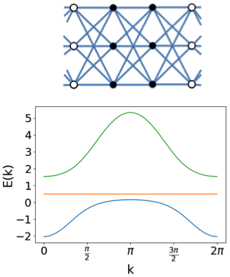
(a)

(b)

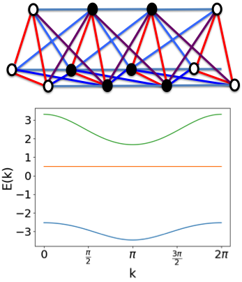
(c)

Figure 1: (Color online) Examples of flat band Hamiltonians with CLS of class $U=2$, $\nu=3$. The sites occupied by a CLS are indicated by filled black circles. Each subfigure contains the visualization of the lattice (top) and the band structure (bottom). The flat band is colored in orange. (a): diagonal $H_{0}$, (b): non-diagonal $H_{0}$, (c): non-diagonal and fully connected $H_{0}$. Appendix D.1 contains the detailed description of the Hamiltonians.

For a bipartite network, the hopping matrix $H_{1}$ has a specific structure given by Eqs. (34), that simplifies Eqs. (42) to

$$S\ket{\varphi_{2}} =-A\ket{\varphi_{1}}$$ (46)

$$S\ket{\varphi_{1}} =0$$ (47)

$$T\ket{\varphi_{1}} =-A\ket{\varphi_{2}}$$ (48)

$$T\ket{\varphi_{2}} =0,$$ (49)

and $E_{\text{FB}}=0$. The minority sublattice hopping matrices $B,W$ dropped out as expected. The above equations are considerably simpler than the generic $U=2$ Eqs. (42): the above system splits into two independent inverse eigenvalue problems for $S$ and $T$. The details of the solution are presented in Appendix B.3, the final answer is

$$S=-\frac{A\ket{\varphi_{1}}\bra{\varphi_{2}}Q_{1}}{\matrixelement{\varphi_{2}}{Q_{1}}{\varphi_{2}}}+K_{S}Q_{12}$$

$$T=-\frac{A\ket{\varphi_{2}}\bra{\varphi_{1}}Q_{2}}{\matrixelement{\varphi_{1}}{Q_{2}}{\varphi_{1}}}+K_{T}Q_{12},$$ (50)

where $K_{T}$ and $K_{S}$ are arbitrary matrices of size $(\nu-\mu)\times\mu$ respectively. The $Q_{12}$ is a joint transverse projector on $\ket{\varphi_{1,2}}$. There are no restrictions on the entries of $A,B,W$ and $\ket{\varphi_{1,2}}$–they are all free parameters–at variance with the generic $U=2$ flat band construction. Therefore the number of free parameters is: $(\nu-\mu)(2\nu+\mu-2)-1$ (see Appendix B.3 for details). The above solution fails for $\matrixelement{\varphi_{2}}{Q_{1}}{\varphi_{2}}=\matrixelement{\varphi_{1}}{Q_{2}}{\varphi_{1}}\equiv 0$, therefore $\ket{\varphi_{2}}\propto\ket{\varphi_{1}}$, the CLS and the flat band are of class $U=1$.

Figure 2 shows an example of a bipartite lattice with $\nu=4$. There are two sites in the unit cell of each sublattice, and $B\neq 0,W\neq 0$. In this example, the parameters $\vec{\varphi}_{2},\vec{\varphi}_{2},A,B,W$ are arbitrarily chosen, and $K_{T}=0,K_{S}=0$ (See details in the Appendix D.1).

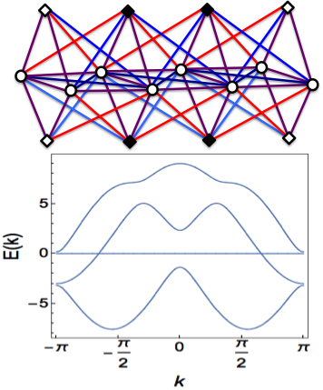
Figure 2: (Color online) Example of a bipartite flat band Hamiltonian with $U=2$, $\nu=4$. The sites of the CLS are indicated by the filled black squares. Links are colored differently for the convenience of visualisation of the chain. In this example the chiral symmetry is broken on the minority sublattice, due to the presence of $B\neq 0,W\neq 0$ in Eq. (34). Nevertheless the chiral flat band is preserved. The details of this example are given in Appendix D.1.

IV.2 $U\geq 3$

Let us consider larger $U$ values. For simplicity we use $U=3$ in the examples. Fix the number of bands to $\nu$, and choose some $H_{0}$, $E_{\text{FB}}$, and $\ket{\psi_{1}}$. Then we have the following inverse eigenvalue problem with $U+2$ equations ($U$ for each CLS occupied unit cell, and two for the destructive interference conditions):

$$H_{1}\ket{\psi_{2}} =\left(E_{\text{FB}}-H_{0}\right)\ket{\psi_{1}}$$

$$H_{1}^{\dagger}\ket{\psi_{1}}+H_{1}\ket{\psi_{3}} =\left(E_{\text{FB}}-H_{0}\right)\ket{\psi_{2}}$$

$$H_{1}^{\dagger}\ket{\psi_{2}} =\left(E_{\text{FB}}-H_{0}\right)\ket{\psi_{3}}$$

$$H_{1}\ket{\psi_{1}} =0$$ (51)

$$H_{1}^{\dagger}\ket{\psi_{3}} =0.$$

The set of constraints for the $\Psi_{\text{CLS}}$ reads

$$\langle\psi_{1}\ket{\psi_{3}}=1$$

$$\matrixelement{\psi_{1}}{H_{0}}{\psi_{3}}=E_{\text{FB}}$$

$$\matrixelement{\psi_{1}}{E_{\text{FB}}-H_{0}}{\psi_{2}}=\matrixelement{\psi_{2}}{E_{\text{FB}}-H_{0}}{\psi_{3}}$$ (52)

$$\matrixelement{\psi_{1}}{E_{\text{FB}}-H_{0}}{\psi_{1}}+\matrixelement{\psi_{3}}{E_{\text{FB}}-H_{0}}{\psi_{3}}=$$

$$=\matrixelement{\psi_{2}}{E_{\text{FB}}-H_{0}}{\psi_{2}}.$$

Again these identities are derived from Eqs. (51) by multiplying them with $\bra{\psi_{1}}$ and $\bra{\psi_{U}}$ and rearranging terms, in order to eliminate $H_{1}$. Notice that the set of compatibility constraints for $\Psi_{\text{CLS}}$ amounts to $U+1$ equations. Note also that in precisely two of those $U+1$ equations, with $\bra{\psi_{1}}$ given, amount to 2 linear, and $U-1$ nonlinear equations for the remaining CLS amplitudes. It is not possible to solve the nonlinear equations analytically in general, but we present in Appendix C.2 a numerical algorithm that allows to resolve these constraints and enumerate all the solutions, if existing, for the case $U=3$.

Instead of using the ansatz (44) for $H_{1}$, we take a more suitable approach to generate flat band Hamiltonians (i.e. matrices $H_{1}$) for $U\geq 3$. With a given $\Psi_{\text{CLS}}$ which satisfies the constraints (52), the set of equations (51) is a linear system with respect to $H_{1}$:

$$T\,h_{1}=\Lambda.$$ (53)

Here $h_{1}$ is a $\nu^{2}$-dimensional vector resulting from the vectorization of the matrix $H_{1}$. $T$ is a rectangular $\nu(U+2)\times\nu^{2}$ matrix whose elements are composed by the elements of CLS, such that the product $T\,h_{1}$ is the left-hand side of Eqs. (51). $\Lambda$ is a $\nu(U+2)$ vector originating from the right-hand side of Eqs. (51):

$$\Lambda=(E_{\text{FB}}-H_{0})\begin{pmatrix}\vec{\psi}_{1}\\ \vec{\psi}_{2}\\ \dots\\ \vec{\psi}_{U}\\ \vec{0}\\ \vec{0}\end{pmatrix}.$$ (54)

The zero vector components $\vec{0}$ result from the destructive interference. The linear system (53) can be then solved, e.g., using a least squares solver. Figure 3 shows some examples of $U=3$ flat bands, which we generated by resolving the constraints (52) and solving Eq. (53).

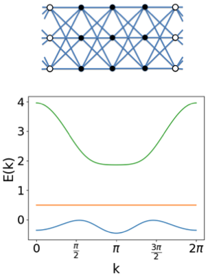
(a)

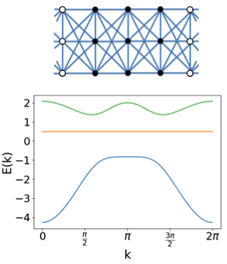
(b)

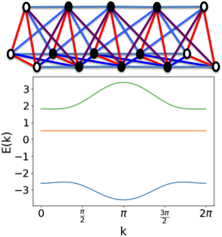
(c)

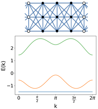
(d)

Figure 3: (Color online) Examples of Hamiltonians with a CLS of class $U=3$. The sites occupied by a CLS are indicated by black filled circles. (a) Diagonal choice for $H_{0}$. (b) Chain like structure for $H_{0}$. (c) Generic choice for $H_{0}$. (d) $E_{FB}$ is chosen negative enough to become the groundstate. Details of these examples are presented in Appendix D.2.

IV.3 Network constraints

For practical purposes, the flat band fine-tuning of a Hamiltonian network can involve additional network constraints, e.g. the strict vanishing of certain hopping terms between specific sites of the network Poli et al. (2017). This typically happens when arranging network sites in a plane. Let us consider the typical problem of finding a nearest-neighbor flat band Hamiltonian with specific network constraints. These network constraints dictate the locations of zero entries in $H_{0}$ and $H_{1}$. They can be incorporated into the matrix $T$ of Eq. (53) as a mask $M$: $T\to TM$ that enforces zero entries in $H_{1}$ in the right positions. The solution of the resulting system is then searched for similar to the non-constrained case.

Especially when $H_{0}$ and $H_{1}$ are sparse , e.g., the number of variables in $H_{1}$ is equal to or greater then the number of equations, it is possible to solve (35)-(39) analytically (see Appendix E). Figure 4 shows examples of networks with flat bands generated for a $d=1$ Kagome chain and chains with hoppings allowed only inside network plaquettes.

(a)

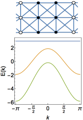
(b)

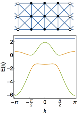
(c)

Figure 4: (Color online) Examples of flat band Hamiltonians constructed on specific networks. The sites occupied by a CLS are marked by black filled circles. (a):1d Kagome with $\nu=5$ and $U=2$ compact localized states. The crossing of three bands indicates that the Hamiltonian can be detangled into two independent sub-Hamiltonians. (b) and (c) Examples of Hamiltonians with $\nu=3$, $U=2$ and $U=3$ CLS, respectively. The details of all these Hamiltonians are provided in Appendix E.

V Conclusions

We presented a systematic construction of one-dimensional Hamiltonians with $\nu$ bands including one flat band for an arbitrary size $U\leq\nu$ of compact localized states and illustrated the method with several examples. The task of finding flat band Hamiltonians is reduced to solving a specific inverse eigenvalue problems subject to certain non-linear constraints. The flat band energy enters as a parameter and can be tuned. For the $U=2$ case we derive analytical solutions to the inverse eigenvalue problem supplemented with a numerical algorithm to resolve for the constraints. For $U\geq 3$ analytical solutions are not accessible, yet numerical algorithms are applied to generate flat band Hamiltonians. We illustrate the method by generating several $U=3$ flat band Hamiltonians. The same construction allows to incorporate various network geometry constraints into the search algorithm. Our results show that flat band Hamiltonians, while being the result of a finetuning in the space of all tight binding Hamiltonian networks, allow for a surprisingly large number of free parameters which change the network, but leave the flatness of the flat band untouched.

Open questions include the extension of the present formalism to the case of multiple flat bands and/or higher dimensions. The present algorithm can be extended naturally to higher dimensions and will generalize the approach of Nishino et al Nishino et al. (2003); Nishino and Goda (2005). The extension to $d=2,3$ would require more intercell hopping matrices $H_{a}$ describing hopping in different dimensions–$H_{x},H_{y}$ in the simplest case of the square lattice geometry–beyond just $H_{1}$. Also the simple classification in terms of the CLS size $U$ has to be extended: one has to specify the shape of the compact localised state. Equations (1) regarded as an inverse eigenvalue problem would now couple different $H_{a}$. These equations can be decoupled with respect to $H_{a}$ by introducing additional variables, and reduced to inverse eigenvalue problems for individual hopping matrices $H_{a}$, similar to the ones that we were solving here for $d=1$.

Another interesting interesting avenue for future research is the case of non-Hermitian Hamiltonians allowing for gain and loss terms in the Hamiltonian (9). Recently a number of works Ge (2018); Leykam et al. (2017b) analyzed flat bands in such systems or considered the fate of flat bands in the presence of non-Hermitian perturbations Ge (2015); Longhi (2019) and finding interesting results. Finally, non-Hermitian Hamiltonians have a larger parameter space suggesting richer classification as compared to the Hermitian case. We expect therefore that a systematic construction and identification of flat bands in this context might lead to new interesting results.

Appendix A Reduction of CLS of class $U$ into $U-1$, when $\vec{\psi}_{1}\perp\vec{\psi}_{U}$.

Suppose we have a CLS of class $U$, that we write as $\vec{\psi}_{cls}=(\vec{\psi}_{1},\vec{\psi}_{2},\dots,\vec{\psi}_{U})^{T}$, and $\vec{\psi}_{1}\perp\vec{\psi}_{U}$. Then we can apply a unitary transformation $R$ on the CLS, such that $\tilde{\vec{\psi}}_{i}=R\vec{\psi}_{i},\ i=1,\dots,U$ and

$$\tilde{\vec{\psi}}_{1}=\begin{bmatrix}1\\ 0\\ \vdots\\ 0\end{bmatrix},\quad\tilde{\vec{\psi}}_{2}=\begin{bmatrix}\psi_{2}^{1}\\ \psi_{2}^{2}\\ \vdots\\ \psi_{2}^{\nu}\end{bmatrix},\dots,\quad\tilde{\vec{\psi}}_{U}=\begin{bmatrix}0\\ \psi_{U}^{2}\\ \vdots\\ \psi_{U}^{\nu}\end{bmatrix},\;$$ (55)

where $\nu$ is number of sites per unit cell. Due to unitary of transformation $R$, the eigenvalue problem (35-39) does not change. Next we redefine the unit cell in the following way

$$\bar{\vec{\psi}}_{1}=\begin{bmatrix}1\\ \psi_{2}^{2}\\ \vdots\\ \psi_{2}^{\nu}\end{bmatrix},\ \bar{\vec{\psi}}_{2}=\begin{bmatrix}\psi_{2}^{1}\\ \psi_{3}^{2}\\ \vdots\\ \psi_{3}^{\nu}\end{bmatrix},\dots,\ \bar{\vec{\psi}}_{U-1}=\begin{bmatrix}\psi_{U-1}^{1}\\ \psi_{U}^{2}\\ \vdots\\ \psi_{U}^{\nu}\end{bmatrix},$$

and $\bar{\vec{\psi}}_{U}=0$. Therefore, after the unitary transformation $R$ and redefinition of the unit cell, the class of the CLS reduces to $U-1$. The schematics of this procedure is shown in Figure 5.

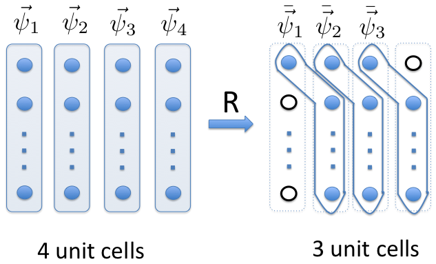
Figure 5: (Color online) A schematics showing how a CLS of class $U=4$ reduces to $U=3$, when $\vec{\psi}_{1}\perp\vec{\psi}_{4}$. Each elongated box stands for one unit cell. Filled circles - nonzero wave function components. Open circles - zero wave function components.

Appendix B Inverse eigenvalue problem: a toy example and the solution of the $U=2$ CLS

This appendix explains the solution of the inverse eigenvalue problems (42). As discussed in main text, 1D flat band lattices with CLS class $U$ satisfy

$$H_{1}\vec{\psi}_{2} =\left(E_{\text{FB}}-H_{0}\right)\vec{\psi}_{1},$$

$$H_{1}^{\dagger}\vec{\psi}_{l-1}+H_{1}\vec{\psi}_{l+1} =\left(E_{\text{FB}}-H_{0}\right)\vec{\psi}_{l}\quad l=2,\dots,U-1,$$

$$H_{1}^{\dagger}\vec{\psi}_{U-1} =\left(E_{\text{FB}}-H_{0}\right)\vec{\psi}_{U},$$

$$H_{1}\vec{\psi}_{1} =0,$$

$$H_{1}^{\dagger}\vec{\psi}_{U} =0.$$ (56)

Assuming that $E_{\text{FB}},H_{0},\vec{\psi}_{l=1,\dots,U}$ are given, the equations (56) constitute an inverse eigenvalue problem for a block-tridiagonal matrix, where diagonal blocks are $H_{0}$ and off diagonal ones are $H_{1}$.

B.1 Toy example

As a warmup, we solve a toy inverse eigenvalue problem: reconstruct $\nu\times\nu$ matrix $T$ given its action $\ket{y}$ on some vector $\ket{x}$

$$T\,\ket{x}=\ket{y}.$$ (57)

The solution is not unique: generic solution can be represented as $T=T_{*}+\delta T$, where $T_{*}$ is any particular solution of Eq. (57) and $\delta T\ket{x}=0$. One possible particular solution is easily found to be

$$T_{*}=\frac{\ket{y}\bra{x}}{\bra{x}\ket{x}},\quad\delta T=Q_{x}\,K,$$ (58)

where $Q_{x}$ is a transverse projector on $x$. This construction generalizes straightforwardly to the case of many vectors (we assume here implicitly that the equations are consistent):

$$T\ket{x_{k}}=\ket{y_{k}}\quad k=1..m.$$ (59)

The generic solution to this problem is given by

$$T_{*}=\sum_{ij}A_{ij}\ket{y_{i}}\bra{x_{j}},\quad A_{ij}^{-1}=\bra{x_{i}}\ket{x_{j}}$$ (60)

$$\delta T=Q\,K,$$ (61)

where $Q$ is the orthogonal projector on the subspace spanned by $\{x_{k}\}$ and $K$ is an arbitrary $\nu\times\nu$ matrix. For later convenience we refer to $T_{*}$ as particular solution and $\delta T$ as free part.

B.2 U=2 case

In this case, Eq. (56) reads

$$H_{1}\ket{\psi_{2}} =\left(E_{\text{FB}}-H_{0}\right)\ket{\psi_{1}}$$

$$H_{1}^{\dagger}\ket{\psi_{1}} =\left(E_{\text{FB}}-H_{0}\right)\ket{\psi_{2}}$$

$$H_{1}\ket{\psi_{1}} =0$$ (62)

$$H_{1}^{\dagger}|\psi_{2}\rangle =0.$$

We know $H_{0},\ket{\psi_{1}},\ket{\psi_{2}}$ and $E_{\text{FB}}=\matrixelement{\psi_{1}}{H_{0}}{\psi_{2}}$, and we need to determine $H_{1}$. As discussed above for the toy case, the generic solution to this problem can be decomposed into a particular solution and a free part. The last two equations in the above set are satisfied by the following ansatz:

$$H_{1}=Q_{2}MQ_{1},\quad Q_{i}=\mathbb{I}-\frac{\ket{\psi_{i}}\bra{\psi_{i}}}{\langle\psi_{i}|\psi_{i}\rangle}.$$ (63)

Plugging this ansatz back into the system, we find

$$Q_{2}\,M\,Q_{1}\ket{\psi_{2}}=\left(E_{\text{FB}}-H_{0}\right)\ket{\psi_{1}}$$ (64)

$$\bra{\psi_{1}}Q_{2}\,M\,Q_{1}=\bra{\psi_{2}}\left(E_{\text{FB}}-H_{0}\right).$$

Note the identity

$$\matrixelement{\psi_{1}}{H_{1}}{\psi_{2}}=\matrixelement{\psi_{1}}{E_{\text{FB}}-H_{0}}{\psi_{1}}=\matrixelement{\psi_{2}}{E_{\text{FB}}-H_{0}}{\psi_{2}},$$ (65)

that follows straightforwardly from the first two equations of (62). Defining the projectors

$$R_{12}=\mathbb{I}-\frac{Q_{1}\ket{\psi_{2}}\bra{\psi_{2}}Q_{1}}{\expectationvalue{Q_{1}}{\psi_{2}}}$$ (66)

$$R_{21}=\mathbb{I}-\frac{Q_{2}\ket{\psi_{1}}\bra{\psi_{1}}Q_{2}}{\expectationvalue{Q_{2}}{\psi_{1}}},$$

we can write

$$M=T+R_{21}\,K\,R_{12},$$ (67)

where $T$ is a particular solution of Eq. (64). The second term, where $K$ is an arbitrary $\nu\times\nu$ matrix, satisfies Eqs. (64) by construction and is the free part of the solution. Therefore we only need to find a particular solution to the system to get the generic solution. This is achieved by the same ansatz $T=\ket{x}\bra{y}$ as in the toy case discussed above. The ansatz yields the following equations:

$$Q_{2}\,T\,Q_{1}\ket{\psi_{2}}=\matrixelement{y}{Q_{1}}{\psi_{2}}Q_{2}\ket{x}=(E_{\text{FB}}-H_{0})\ket{\psi_{1}}$$ (68)

$$\bra{\psi_{1}}Q_{2}\,T\,Q_{1}=\matrixelement{\psi_{1}}{Q_{2}}{x}\bra{y}Q_{1}=\bra{\psi_{2}}(E_{\text{FB}}-H_{0}).$$ (69)

From these the vectors $x$ and $y$ are fixed (up to unimportant normalization):

$$\bra{y}Q_{1}=\frac{1}{\matrixelement{\psi_{1}}{Q_{2}}{x}}\bra{\psi_{2}}(E_{\text{FB}}-H_{0})$$

$$Q_{2}\ket{x}=\frac{1}{\matrixelement{y}{Q_{1}}{\psi_{2}}}(E_{\text{FB}}-H_{0})\ket{\psi_{1}}$$

$$=\frac{\matrixelement{\psi_{1}}{Q_{2}}{x}}{\matrixelement{\psi_{2}}{E_{\text{FB}}-H_{0}}{\psi_{2}}}(E_{\text{FB}}-H_{0})\ket{\psi_{1}}$$

$$=\frac{\matrixelement{\psi_{1}}{Q_{2}}{x}}{\matrixelement{\psi_{1}}{E_{\text{FB}}-H_{0}}{\psi_{1}}}(E_{\text{FB}}-H_{0})\ket{\psi_{1}}.$$

We used the condition (65) to replace the denominator in the fourth line. Also note that the expression for $y$ from the first line was used to simplify the second line, and eliminate $y$. The particular solution is then

$$Q_{2}TQ_{1}=\frac{\left(E_{\text{FB}}-H_{0}\right)\ket{\psi_{1}}\bra{\psi_{2}}\left(E_{\text{FB}}-H_{0}\right)}{\matrixelement{\psi_{1}}{E_{\text{FB}}-H_{0}}{\psi_{1}}}$$ (70)

Thanks to (65) it is symmetric with respect to $\ket{\psi_{1}},\ket{\psi_{2}}$. This and the above mentioned free part $Q_{21}KQ_{12}$ give the full family of solutions (45):

$$H_{1}=\frac{(E_{\text{FB}}-H_{0})\ket{\psi_{1}}\bra{\psi_{2}}(E_{\text{FB}}-H_{0})}{\matrixelement{\psi_{1}}{E_{\text{FB}}-H_{0}}{\psi_{1}}}+Q_{2}R_{21}KR_{12}Q_{1}$$

This expression is further simplified by noticing that $R_{12}Q_{1}$ and $Q_{2}R_{21}$ are the same projector on the subspace spanned by $\ket{\psi_{1}},\ket{\psi_{2}}$, that we denote $Q_{12}$: $(R_{12}Q_{1})^{2}=R_{12}Q_{1}$, idem for $Q_{2}R_{21}$ and both vanish when acting on $\ket{\psi_{1,2}}$ as can be straightforwardly verified. We can therefore replace these combinations by $Q_{12}$:

$$H_{1}=\frac{(E_{\text{FB}}-H_{0})\ket{\psi_{1}}\bra{\psi_{2}}(E_{\text{FB}}-H_{0})}{\matrixelement{\psi_{1}}{E_{\text{FB}}-H_{0}}{\psi_{1}}}+Q_{12}KQ_{12}.$$ (71)

This solution is supplemented by the following non-linear constraints

$$\langle\psi_{2}|\psi_{1}\rangle =1$$ (72)

$$\matrixelement{\psi_{2}}{H_{0}}{\psi_{1}} =E_{\text{FB}}$$

$$\matrixelement{\psi_{1}}{E_{\text{FB}}-H_{0}}{\psi_{1}} =\matrixelement{\psi_{2}}{E_{\text{FB}}-H_{0}}{\psi_{2}},$$

that are obtained by eliminating $H_{1}$ from Eq. (62) using ”destructive interference conditions”, i.e. last two equations in Eq. (62).

In case the denominator in Eq. (71) is zero, the single projector ansatz fails, and two projector ansatz has to be used:

$$H_{1} =\frac{(E_{\text{FB}}-H_{0})\ket{\psi_{1}}\bra{\psi_{2}}Q_{1}}{\matrixelement{\psi_{2}}{Q_{1}}{\psi_{2}}}$$ (73)

$$+\frac{Q_{2}\ket{\psi_{1}}\bra{\psi_{2}}(E_{\text{FB}}-H_{0})}{\matrixelement{\psi_{1}}{Q_{2}}{\psi_{1}}}+Q_{12}KQ_{12},$$

as can be verified by a direct substitution. In this special solution the denominators only vanish when $\Psi_{1}\propto\Psi_{2}$, i.e. in $U=1$ case.

B.3 Bipartite lattices and chiral symmetry

In this section we solve the inverse eigenvalue problem for $U=2$ for the special case of bipartite lattices. We consider a bipartite lattice with $\nu$ sites per unit cell that split into majority and minority sublattices with $\mu$ and $\nu-\mu$ sites respectively. Since the lattice is bipartite, the sites on one sublattice only have neighbours belonging to the other sublattice. This enforces the following structure on the hopping matrices and the wave functions of the CLS (see Eqs. (34)):

$$H_{0}=\left(\begin{array}[]{cc}0&A^{\dagger}\\ A&B\end{array}\right),\quad H_{1}=\left(\begin{array}[]{cc}0&T^{\dagger}\\ S&W\end{array}\right),$$ (78)

$$\vec{\psi}_{1}=\left(\begin{array}[]{c}\varphi_{1}\\ 0\end{array}\right),\quad\vec{\psi}_{2}=\left(\begin{array}[]{c}\varphi_{2}\\ 0\end{array}\right).$$ (83)

Here $\varphi_{1,2}$ are $\mu$ component vectors describing the wave amplitudes of the majority sublattice sites. $A,S,T$ are $(\nu-\mu)\times\mu$ matrices, while $B,W$ are $(\nu-\mu)\times(\nu-\mu)$ matrices. $B,W$ formally break the bipartiteness of the lattice, but do not affect the $E_{\text{FB}}=0$ flat band(s). This special structure simplifies Eqs. (62):

$$S\ket{\varphi_{2}}=-A\ket{\varphi_{1}}$$ (84)

$$T\ket{\varphi_{1}}=-A\ket{\varphi_{2}}$$ (85)

$$S\ket{\varphi_{1}}=0$$ (86)

$$T\ket{\varphi_{2}}=0.$$ (87)

These equations need to be resolved with respect to $S$ and $T$. The last two equations are satisfied by the ansätse $S=S^{\prime}Q_{1}$, $T=T^{\prime}Q_{2}$, where $Q_{i}$ is a transverse projector on $\varphi_{i}$. The remaining two equations are identical to the toy problem that we discussed above(see Appendix B.1) and their solution is precisely Eqs. (50):

$$S=-\frac{A\ket{\varphi_{1}}\bra{\varphi_{2}}Q_{1}}{\matrixelement{\varphi_{2}}{Q_{1}}{\varphi_{2}}}+K_{S}Q_{12}$$ (88)

$$T=-\frac{A\ket{\varphi_{2}}\bra{\varphi_{1}}Q_{2}}{\matrixelement{\varphi_{1}}{Q_{2}}{\varphi_{1}}}+K_{T}Q_{12},$$

where $Q_{12}$ is a joint transverse projector on $\ket{\varphi_{1,2}}$.

Now let’s count the number of free parameters. $|\varphi_{1}\rangle,|\varphi_{2}\rangle$ all are free parameters each contains $\mu$ free parameters. $A$ contains $(\nu-\mu)\mu$ free variables. $B,W$ each contains $(\nu-\mu)^{2}$ free parameters. $K_{S}Q_{12}$ and $Q_{21}K_{T}$ are $(\nu-\mu)\times\mu$ and $\mu\times(\nu-\mu)$ matrices, and, because of the transverse projectors, they contain $(\nu-\mu)(\mu-2)$ and $\mu(\nu-\mu-2)$ free parameters respectively. Therefore total number of free parameters in the solution (88) contains $2\mu-1+(\nu-\mu)\mu+(\nu-\mu)(\mu-2)+\mu(\nu-\mu-2)+2(\nu-\mu)^{2}=(\nu-\mu)(2\nu+\mu-2)-1$ free parameters. The extra $-1$ corresponds to the overall normalisation of the CLS, that is not fixed.

Appendix C Resolving the non-linear constraints

Let us discuss how one can efficiently resolve the set of non-linear constraints, that appear in the inverse eigenvalue problem, for example (72). Since these are a non-linear system of equations, one can always try a numerical solver. However our experience was not particularly successful: the solver was not converging and finding no solution more often than not. Instead it is possible to design an numerical algorithm that eliminates constraints one by one and either founds and enumerates all the solutions, or proves that there are none.

C.1 U=2 case

The non-linear equations that we need to solve are:

$$\langle\psi_{1}|\psi_{2}\rangle =1$$ (90)

$$\matrixelement{\psi_{1}}{H_{0}}{\psi_{2}} =E_{\text{FB}}$$ (91)

$$\expectationvalue{E_{\text{FB}}-H_{0}}{\psi_{1}} =\expectationvalue{E_{\text{FB}}-H_{0}}{\psi_{2}}.$$ (92)

We assume that $E_{\text{FB}}$, $H_{0}$ and $\psi_{1}$ (or $\psi_{2}$) are given input parameters.

Then we need to solve the above equations for $\psi_{2}$. The first two equations (90-91) are linear and are easily satisfied with the following expansion for $\psi_{2}$, by the choice of the basis vectors $e_{1}$ and $e_{2}$:

$$\ket{\psi_{2}}=\sum_{k=1}^{\nu}x_{k}\ket{e_{k}}$$ (93)

$$\ket{e_{1}}=\frac{1}{\sqrt{\bra{\psi_{1}}\ket{\psi_{1}}}}\ket{\psi_{1}}$$ (94)

$$\ket{e_{2}}=\frac{1}{\sqrt{\matrixelement{\psi_{1}}{H_{0}Q_{1}H_{0}}{\psi_{1}}}}Q_{1}H_{0}\ket{\psi_{1}}$$ (95)

$$\bra{e_{l}}\ket{e_{m}}=\delta_{lm},\quad l,m=1,2,\dots\nu.$$ (96)

Here $Q_{1}$ is a transverse projector on $\ket{\psi_{1}}$. With this choice of the basis vectors the equations (90-91) imply:

$$x_{1}=\frac{1}{\sqrt{\bra{\psi_{1}}\ket{\psi_{1}}}},$$

$$x_{2}=\frac{1}{\sqrt{\matrixelement{\psi_{1}}{H_{0}Q_{1}H_{0}}{\psi_{1}}}}\left[E_{\text{FB}}-\frac{\matrixelement{\psi_{1}}{H_{0}}{\psi_{1}}}{\bra{\psi_{1}}\ket{\psi_{1}}}\right].$$

The remaining basis vectors are fixed by requiring their orthonormality, for example, by using Gram-Schmidt orthogonalization. Next we plug the expansion (93) into Eq. (92) and separate out the terms with $e_{1}$, $e_{2}$:

$$\expectationvalue{E_{\text{FB}}-H_{0}}{\psi_{1}}=\sum_{ij=1}^{\nu}x_{i}^{*}x_{j}\matrixelement{e_{i}}{E_{\text{FB}}-H_{0}}{e_{j}}$$

$$=\sum_{ij=1}^{2}x_{i}^{*}x_{j}\matrixelement{e_{i}}{E_{\text{FB}}-H_{0}}{e_{j}}$$

$$+\sum_{i=1}^{2}\sum_{j=3}^{\nu}\left[x_{i}^{*}x_{j}\matrixelement{e_{i}}{E_{\text{FB}}-H_{0}}{e_{j}}+x_{j}^{*}x_{i}\matrixelement{e_{j}}{E_{\text{FB}}-H_{0}}{e_{i}}\right]$$

$$+\sum_{ij=3}^{\nu}x_{i}^{*}x_{j}\matrixelement{e_{i}}{E_{\text{FB}}-H_{0}}{e_{j}}.$$

This expression can be rewritten as follows:

$$\sum_{ij=1}^{\nu-2}y_{i}^{*}M_{ij}y_{j}+\sum_{i=1}^{\nu-2}\left[u_{i}^{*}y_{i}+u_{i}y_{i}^{*}\right]=w$$ (97)

$$M_{ij}=\matrixelement{e_{i+2}}{E_{\text{FB}}-H_{0}}{e_{j+2}}$$ (98)

$$u_{i}=\sum_{j=1}^{2}x_{j}\matrixelement{e_{i+2}}{E_{\text{FB}}-H_{0}}{e_{j}}$$ (99)

$$w=\sum_{ij=1}^{2}x_{i}^{*}x_{j}\matrixelement{e_{i}}{E_{\text{FB}}-H_{0}}{e_{j}}-\expectationvalue{E_{\text{FB}}-H_{0}}{\psi_{1}},$$ (100)

where $y_{i}=x_{i+2}$. The equations on $y_{i}$ are further simplified by the shift: $z_{i}=y_{i}+M_{ij}^{-1}u_{j}$, that eliminates the linear term. This gives the following equation on a quadratic form

$$\sum_{ij=1}^{\nu-2}z_{i}^{*}M_{ij}z_{j}=w+\sum_{ij=1}^{\nu-2}u_{i}^{*}M_{ij}u_{j}$$ (101)

Notice that the RHS of the above equation is real. The matrix $M$ is Hermitian, and can be diagonalized: $M_{ij}=\sum_{\alpha}E_{\alpha}\ket{r_{\alpha}}\bra{r_{\alpha}}$. The above equation is solved with the help of this spectral decomposition:

$$\sum_{\alpha=1}^{\nu-2}E_{\alpha}|t_{\alpha}|^{2}=\tilde{w}$$ (102)

$$\tilde{w}=w+\sum_{\alpha=1}^{\nu-2}E_{\alpha}|s_{\alpha}|^{2}$$ (103)

$$t_{\alpha}=\bra{r_{\alpha}}\ket{z_{\alpha}}\qquad s_{\alpha}=\bra{r_{\alpha}}\ket{u}.$$ (104)

The presence or absence of solution is decided by the mutual signs of $\tilde{w}$ and $E_{\alpha}$: if $\tilde{w}>0$ and $E_{\alpha}<0$ $\forall\alpha$, then there is no solution. If one $E_{\alpha}>0$, there is a single solution, for two and more $E_{\alpha}>0$ there is a multiparametric family of solutions. Knowing $t_{\alpha}$, it is straightforward to reconstruct the original $\vec{\psi}_{2}$.

In the above $M$ was assumed non-singular. If it is singular, than $M_{ij}^{-1}$ is the Moore-Pensrose pseudoinverse Ben-Israel and Greville (2003) and we have $y_{i}=z_{i}+g_{i}-M_{ij}^{-1}u_{j}$ where $g\in\ker{M}$. For $g_{i}$ the quadratic terms in (97) vanish (by definition of $g_{i}$) and the $g_{i}$ only enter linearly the equation, while $z_{i}$ can be treated as in the non-singular case (for convenience we assume that the first $k$ eigenvalues of $M$ are zero):

$$\sum_{\alpha=k+1}^{\nu-2}E_{\alpha}t_{\alpha}^{2}=\tilde{w}-\sum_{\alpha=1}^{k}\left[\bra{u}\ket{r_{\alpha}}+\bra{r_{\alpha}}\ket{u}\right].$$ (105)

The presence of zero modes renormalizes $\tilde{w}$.

The more refined version of the counting relies on the above solution, and the counting of the $E_{\alpha}$ with the “right” sign. It tells us that for $\nu=2,3$, there is a single solution for fixed $\vec{\psi}_{1},E_{\text{FB}},H_{0}$. For larger $\nu$, there could be a single solution or multiparametric families of solutions, from $0$ to $\nu-3$.

C.2 U=3 case

In this case the nonlinear constraints read, Eq. (52):

$$\langle\psi_{1}|\psi_{3}\rangle=1$$

$$\matrixelement{\psi_{1}}{H_{0}}{\psi_{3}}=E_{\text{FB}}$$

$$\matrixelement{\psi_{1}}{E_{\text{FB}}-H_{0}}{\psi_{2}}=\matrixelement{\psi_{2}}{E_{\text{FB}}-H_{0}}{\psi_{3}}$$ (106)

$$\matrixelement{\psi_{3}}{E_{\text{FB}}-H_{0}}{\psi_{3}}=\matrixelement{\psi_{2}}{E_{\text{FB}}-H_{0}}{\psi_{2}}$$

$$-\matrixelement{\psi_{1}}{E_{\text{FB}}-H_{0}}{\psi_{1}}$$

The resolution of this set of constraint is very similar to the $U=2$ case, therefore we only outline the main steps. We search to resolve the above equations with respect to $\Psi_{3}$, taking $\Psi_{1},\Psi_{2}$ as inputs. The first $3$ equations are linear, and we solve them by expanding $\Psi_{3}$ over a suitable orthonormal basis:

$$\ket{\psi_{3}} =\sum_{k}x_{k}\ket{e_{k}},$$

$$\ket{e_{1}} =\frac{1}{\sqrt{\bra{\psi_{1}}\ket{\psi_{1}}}}\ket{\psi_{1}},$$

$$\ket{e_{2}} =\frac{1}{\sqrt{\matrixelement{\psi_{1}}{H_{0}Q_{1}H_{0}}{\psi_{1}}}}Q_{1}H_{0}\ket{\psi_{1}},$$

$$\ket{e_{3}} =\frac{Q_{*}(E_{\text{FB}}-H_{0})\ket{\psi_{2}}}{\sqrt{\matrixelement{\psi_{2}}{(E_{\text{FB}}-H_{0})Q_{*}(E_{\text{FB}}-H_{0})}{\psi_{2}}}},$$

$$\vdots$$

$$\bra{e_{l}}\ket{e_{m}} =\delta_{l,m},\ \ l,m=1,2,\dots,\nu$$

$$Q_{1} =\mathbb{I}-\frac{\ket{\psi_{1}}\bra{\psi_{1}}}{\bra{\psi_{1}}\ket{\psi_{1}}},$$

and $Q_{*}$ is a joint transverse projector on $\ket{\psi_{1}}$ and $Q_{1}H_{0}\ket{\psi_{1}}$. Then $x_{1}$ and $x_{2}$ are the same as in the $U=2$ case, $x_{3}$ is directly expressed through the third equation in Eqs. (106). The last, fourth equation in (106) is solved in the same way as that in the $U=2$ case: it is reduced to solving a quadratic form.

Appendix D Examples for FB generators

In this section we present the details of the example flat band Hamiltonians generated using the algorithm discussed in the main text. In all of these examples we pick some $H_{0},E_{\text{FB}}$ and part of the $\psi_{l}$ as an input. Next following the algorithm outlined in the Appendix C we construct a set of $\{\psi_{l}\}$ consistent with the CLS structure. Then we find the hopping matrix $H_{1}$ using the algorithm from Section III.2 (detailed in Appendix B). For simplicity we drop the free part $K$ in all the examples below.

D.1 $\nu=3,U=2$ case

Example shown in Fig. 1a: We start with a three band case $\nu=3$, and no additional constraints on the form of $H_{1}$. We assume canonical (diagonal) form of $H_{0}$ and choose $\vec{\psi}_{1}$

$$H_{0}=\left[\begin{array}[]{ccc}0&0&0\\ 0&1&0\\ 0&0&2\end{array}\right],\ \ \vec{\psi}_{1}=\left(1,-1,1\right),$$ (110)

Using the FB algorithm, we find the particular solution:

$$E_{\text{FB}}=0.5,\quad\vec{\psi}_{2}=\left(1.5,\ 1.5,\ 1\right)$$ (111)

$$H_{1}=\left[\begin{array}[]{ccc}-0.25&0.25&0.5\\ -0.25&0.25&0.5\\ 0.75&-0.75&-1.5\end{array}\right],$$ (115)

Example shown in Figure 1b: Taking non-diagonal $H_{0}$ and $\vec{\psi}_{1}$ as

$$H_{0}=\left[\begin{array}[]{ccc}0&1&0\\ 1&0&1\\ 0&1&0\end{array}\right],\ \ \vec{\psi}_{1}=\left(1,-1,1\right),$$ (119)

we construct the following FB Hamiltonian:

$$H_{1}=\left[\begin{array}[]{ccc}0.19926929&-0.47727273&-0.67654202\\ -0.33211549&0.79545455&1.12757003\\ 0.19926929&-0.47727273&-0.67654202\end{array}\right],$$ (123)

$$\vec{\psi}_{2}=\left(4.46130814,\ 1.5,\ -1.96130814\right),\ E_{\text{FB}}=0.5$$ (124)

Example shown in Figure 1c: Taking all the sites in the unit cell connected to each other and the same $\vec{\psi}_{1}$, $E_{\text{FB}}$ as in the above example

$$H_{0}=\left[\begin{array}[]{ccc}0&1&1\\ 1&0&1\\ 1&1&0\end{array}\right],\ \ \vec{\psi}_{1}=\left(1,-1,1\right)$$ (128)

we land at the following Hamiltonian:

$$H_{1}=\left[\begin{array}[]{ccc}0.18163216&-0.16071429&-0.34234644\\ -0.90816078&0.80357143&1.71173221\\ 0.18163216&-0.16071429&-0.34234644\end{array}\right],$$ (132)

$$\vec{\psi}_{2}=\left(1.84761673,\ 0.25,\ -0.59761673\right),\ E_{\text{FB}}=0.5$$ (133)

Bipartite lattice $U=2$, Figure 2: We consider the $\nu=4,\mu=2$ case and pick the following input variables:

$$A=\frac{1}{4}\left(\begin{array}[]{cc}\sqrt{3}&1\\ 3&\sqrt{3}\\ \end{array}\right),\ \ B=\left(\begin{array}[]{cc}1&-2\\ -2&1\\ \end{array}\right)$$

$$\vec{\varphi}_{1}=\frac{1}{\sqrt{2}}\left(1,1\right),\ \ \vec{\varphi}_{2}=\frac{1}{2}\left(1,\sqrt{3}\right)$$

$$W=\left(\begin{array}[]{cc}2&-1\\ -1&2\\ \end{array}\right).$$

Solving Eqs. (50)/(88) yields the following solution:

$$S=\frac{\left(\sqrt{3}+2\right)\left(\begin{array}[]{cc}-1&1\\ -\sqrt{3}&\sqrt{3}\\ \end{array}\right)}{2\sqrt{2}},$$

$$T=\frac{\left(\sqrt{3}+1\right)\left(\begin{array}[]{cc}3&3\sqrt{3}\\ -\sqrt{3}&-3\\ \end{array}\right)}{4\sqrt{2}}$$

The corresponding hopping matrices $H_{0},H_{1}$ read

$$H_{0} =\left(\begin{array}[]{cccc}0&0&\frac{\sqrt{3}}{4}&\frac{3}{4}\\ 0&0&\frac{1}{4}&\frac{\sqrt{3}}{4}\\ \frac{\sqrt{3}}{4}&\frac{1}{4}&1&-2\\ \frac{3}{4}&\frac{\sqrt{3}}{4}&-2&1\\ \end{array}\right)$$

$$H_{1} =\left(\begin{array}[]{cccc}0&T\\ S&W\\ \end{array}\right)$$

$$\vec{\psi}_{1} =\left(\frac{1}{\sqrt{2}},\frac{1}{\sqrt{2}},0,0\right)$$

$$\vec{\psi}_{2} =\left(\frac{1}{2},\frac{\sqrt{3}}{2},0,0\right).$$

D.2 $\nu=3$, $U=3$ case

Example shown in Figure 3a: We pick $H_{0}$ in canonical form and choose $\vec{\psi}_{1}$ as follows

$$H_{0}=\left[\begin{array}[]{ccc}0&0&0\\ 0&1&0\\ 0&0&2\end{array}\right],\ \ \vec{\psi}_{1}=\left(1,-1,1\right)$$

Solving the non-linear constraints (52)/(106), we get $\vec{\psi}_{2},\vec{\psi}_{3}$. Then solving the equation (53), which is equivalent to equations (35-39), we get

$$H_{1} =\left[\begin{array}[]{ccc}-0.06548573&-0.27210532&-0.2066196\\ -0.15130619&-0.28682832&-0.13552213\\ -0.14682469&0.75742396&0.90424865\end{array}\right]$$

$$\vec{\psi}_{2} =\left(-0.05144152,-1.53640189,-0.38025523\right)$$

$$\vec{\psi}_{3} =\left(0.58333333,-0.33333333,0.08333333\right)$$

$$E_{\text{FB}} =0.5$$

Example shown in Figure 3b: We choose $H_{0}$ and $\vec{\psi}_{1}$ as

$$H_{0}=\left[\begin{array}[]{ccc}0&-1&0\\ -1&0&1\\ 0&1&0\end{array}\right],\ \ \vec{\psi}_{1}=\left(1,-1,1\right)$$

The corresponding flat band $H_{1}$ is

$$H_{1} =\left[\begin{array}[]{ccc}0.23624218&0.15535892&-0.08088326\\ -0.87350793&-0.69073091&0.18277702\\ 1.31303601&0.95651792&-0.35651809\end{array}\right]$$

$$\vec{\psi}_{2} =\left(3.14189192,-2.05220768,-0.94681365\right)$$

$$\vec{\psi}_{3} =\left(1.08333333,-0.33333333,-0.41666667\right)$$

$$E_{\text{FB}} =0.5$$

Example shown in Figure 3c: For the following input

$$H_{0}=\left[\begin{array}[]{ccc}0&-1&2\\ -1&0&1\\ 2&1&0\end{array}\right],\ \ \vec{\psi}_{1}=\left(1,-1,1\right),$$

we find the flat band n.n. hopping matrix $H_{1}$:

$$H_{1} =\left[\begin{array}[]{ccc}0.06915801&-0.66620419&-0.7353622\\ -0.31644957&-0.3029663&0.01348327\\ -0.46657738&-0.38011423&0.08646314\end{array}\right]$$

$$\vec{\psi}_{2} =\left(0.77717503,2.50899893,1.05355773\right)$$

$$\vec{\psi}_{3} =\left(0.03571429,-0.57142857,0.39285714\right)$$

$$E_{\text{FB}} =0.5.$$

Example shown in Figure 3d: The following input data

$$H_{0}=\left[\begin{array}[]{ccc}0&1&0\\ 1&0&1\\ 0&1&0\end{array}\right],\ \ \vec{\psi}_{1}=\left(1,-1,1\right),$$

provides an example of the flat band Hamiltonian, with the flat band being the ground state:

$$H_{1} =\left[\begin{array}[]{ccc}-0.52279625&0.17024672&0.69304298\\ -0.62702148&-0.11461122&0.51241027\\ -0.73124671&-0.39946915&0.33177756\end{array}\right]$$

$$\vec{\psi}_{2} =\left(0.25537008,0.28652804,-0.59920373\right)$$

$$\vec{\psi}_{3} =\left(0.25,-0.5,0.25\right)$$

$$E_{\text{FB}} =-1.5.$$

Appendix E Network constraints

We present here the details of the examples where the network connectivity was provided as an input to the FB generator. In all cases one can find particular solutions to the resulting non-linear system of equations.

Often network connectivity implies sparse $H_{0}$ and $H_{1}$ very sparse. Therefore inserting these sparse $H_{0}$ and $H_{1}$ into equations (35-39) gives a set of equations that can be solved analytically. More precisely, as you will see in the examples below, when $H_{0}$ and $H_{1}$ are so sparse that the number unknowns (non-zero elements of $H_{1},H_{0}$ and part of CLS) is less then or equal to the number of equations, we can solve the equations (35-39) analytically. Note that, instead of inserting $H_{1}$ and $H_{0}$ into equations (35-39), we can get the same set of equations from equation (53) by zeroing the elements of $h_{1}$ corresponding to zero elements of $H_{1}$.

E.1 U=2 Case

E.1.1 1D Kagome

We consider the $d=1$ version of the 2D Kagome lattice. The n.n. Hamiltonian is restricted by the lattice connectivity to

$$H_{0}=\left[\begin{array}[]{ccccc}0&t_{2}&0&0&0\\ t_{2}&0&t_{1}&0&0\\ 0&t_{1}&0&t_{1}&0\\ 0&0&t_{1}&0&t_{2}\\ 0&0&0&t_{2}&0\end{array}\right],\ \ H_{1}=\left[\begin{array}[]{ccccc}0&t_{1}&t_{1}&0&0\\ 0&0&0&0&0\\ 0&0&0&0&0\\ 0&0&0&0&0\\ 0&0&t_{1}&t_{1}&0\end{array}\right]$$

The ”destructive interference” condition (17) ,i.e. the last two equations in (42), implies that

$$\vec{\psi}_{1}=\left(x_{1},-x_{2},x_{2},-x_{2},x_{3}\right),\ \ \vec{\psi}_{2}=\left(0,a,b,c,0\right).$$

If we insert $\vec{\psi}_{1},\vec{\psi}_{2}$ above into the equations (42), we find

$$\left(\begin{array}[]{c}-x_{2}t_{2}+\left(y_{2}+y_{3}\right)t_{1}\\ x_{2}t_{1}+x_{1}t_{2}\\ -2x_{2}t_{1}\\ x_{2}t_{1}+x_{3}t_{2}\\ -x_{2}t_{2}+\left(y_{3}+y_{4}\right)t_{1}\end{array}\right) =E_{FB}\left(\begin{array}[]{c}x_{1}\\ -x_{2}\\ x_{2}\\ -x_{2}\\ x_{3}\end{array}\right)$$

$$\left(\begin{array}[]{c}at_{2}\\ \left(b+y_{1}\right)t_{1}\\ \left(a+c+y_{1}+y_{5}\right)\\ \left(b+y_{5}\right)t_{1}\\ ct_{2}\end{array}\right) =E_{FB}\left(\begin{array}[]{c}0\\ a\\ b\\ c\\ 0\end{array}\right)$$

One the possible solutions of above equation is

$$a=c =0$$

$$t_{1} =-\frac{E_{FB}}{2}$$

$$t_{2} =\frac{E_{FB}}{2}$$

$$x_{1} =-x$$

$$x_{2} =x$$

$$x_{3} =-x$$

$$a =0$$

$$b =x$$

$$c =0$$

This solution gives a flat band with energy $E_{FB}$. Thus the final solution is

$$\vec{\psi}_{1} =\left(-x,-x,x,-x,-x\right)$$

$$\vec{\psi}_{2} =\left(0,0,x,0,0\right)$$

$$H_{1} =\left[\begin{array}[]{ccccc}0&-\frac{E_{FB}}{2}&-\frac{E_{FB}}{2}&0&0\\ 0&0&0&0&0\\ 0&0&0&0&0\\ 0&0&0&0&0\\ 0&0&-\frac{E_{FB}}{2}&-\frac{E_{FB}}{2}&0\end{array}\right]$$

$$H_{0} =\left[\begin{array}[]{ccccc}0&\frac{E_{FB}}{2}&0&0&0\\ \frac{E_{FB}}{2}&0&-\frac{E_{FB}}{2}&0&0\\ 0&-\frac{E_{FB}}{2}&0&-\frac{E_{FB}}{2}&0\\ 0&0&-\frac{E_{FB}}{2}&0&\frac{E_{FB}}{2}\\ 0&0&0&\frac{E_{FB}}{2}&0\end{array}\right]$$

This lattice has a flat band with flat band energy $E_{FB}$.

E.1.2 $U=2$, $\nu=3$ example

The connectivity of the network shown in Figure 4b implies the following hopping matrices:

$$H_{0}=\left(\begin{array}[]{ccc}0&t_{1}&0\\ t_{1}&0&t_{2}\\ 0&t_{2}&0\\ \end{array}\right),\ \ H_{1}=\left(\begin{array}[]{ccc}s_{1}&s_{2}&0\\ s_{4}&s_{5}&s_{6}\\ 0&s_{7}&s_{8}\\ \end{array}\right)$$

We parameterize the CLS amplitudes as follows: $\vec{\psi}_{1}=(x,y,z),\vec{\psi}_{2}=(a,b,c)$. Then equations (42) gives

$$\left(\begin{array}[]{c}as_{1}+bs_{2}\\ as_{4}+bs_{5}+cs_{6}\\ bs_{7}+cs_{8}\end{array}\right)=\left(\begin{array}[]{c}xE_{\text{FB}}-t_{1}y\\ -t_{1}x-t_{2}z+yE_{\text{FB}}\\ zE_{\text{FB}}-t_{2}y\end{array}\right)$$

$$\left(\begin{array}[]{c}s_{1}x+s_{4}y\\ s_{2}x+s_{5}y+s_{7}z\\ s_{6}y+s_{8}z\end{array}\right)=\left(\begin{array}[]{c}aE_{\text{FB}}-bt_{1}\\ -at_{1}+bE_{\text{FB}}-ct_{2}\\ cE_{\text{FB}}-bt_{2}\end{array}\right)$$

$$\left(\begin{array}[]{c}s_{1}x+s_{2}y\\ s_{4}x+s_{5}y+s_{6}z\\ s_{7}y+s_{8}z\end{array}\right)=\left(\begin{array}[]{c}0\\ 0\\ 0\end{array}\right)$$

$$\left(\begin{array}[]{c}as_{1}+bs_{4}\\ as_{2}+bs_{5}+cs_{7}\\ bs_{6}+cs_{8}\end{array}\right)=\left(\begin{array}[]{c}0\\ 0\\ 0\end{array}\right)$$

Here $H_{0}$, $E_{\text{FB}}$ and $\vec{\psi}_{1}$ as free parameters. If we fix $x=1,y=2,z=1,t_{1}=1,t_{2}=2,E_{\text{FB}}=3$, then we find one particular solution of above equations

$$s_{1}=\frac{2\sqrt{2}}{3},\ \ s_{2}=-\frac{\sqrt{2}}{3}$$

$$s_{4}=\frac{2\sqrt{2}}{3},\ \ s_{5}=\frac{\sqrt{2}}{3}$$

$$s_{6}=-\frac{1}{3}\left(4\sqrt{2}\right),\ \ s_{7}=-\frac{\sqrt{2}}{3},$$

$$s_{8}=\frac{2\sqrt{2}}{3},\ \ a=\frac{1}{\sqrt{2}}$$

$$b=-\frac{1}{\sqrt{2}},\ \ c=-\sqrt{2}$$

from which follow the hopping matrices and the CLS amplitudes

$$H_{0}=\left(\begin{array}[]{ccc}0&1&0\\ 1&0&2\\ 0&2&0\\ \end{array}\right),\ \ H_{1}=\left(\begin{array}[]{ccc}\frac{2\sqrt{2}}{3}&-\frac{\sqrt{2}}{3}&0\\ \frac{2\sqrt{2}}{3}&\frac{\sqrt{2}}{3}&-\frac{1}{3}\left(4\sqrt{2}\right)\\ 0&-\frac{\sqrt{2}}{3}&\frac{2\sqrt{2}}{3}\\ \end{array}\right)$$

$$\vec{\psi}_{1}=(1,2,1),\ \ \vec{\psi}_{2}=\left(\frac{1}{\sqrt{2}},-\frac{1}{\sqrt{2}},-\sqrt{2}\right).$$

E.2 U=3 case

E.2.1 $U=3$, $\nu=3$ example

We consider networks shown in Fig. 4c. Its connectivity requires the following hopping matrices

$$H_{0}=\left(\begin{array}[]{ccc}0&t_{1}&0\\ t_{1}&0&t_{2}\\ 0&t_{2}&0\\ \end{array}\right),\ \ H_{1}=\left(\begin{array}[]{ccc}s_{1}&s_{1}&0\\ -\frac{s_{1}}{2}&-\frac{s_{1}}{2}-s_{6}&s_{6}\\ 0&2s_{6}&-2s_{6}\\ \end{array}\right)$$

According to ”destructive interference” condition (17), we paramterize $\vec{\psi}_{1},\vec{\psi}_{2},\vec{\psi}_{3}$ as follows

$$\vec{\psi}_{1}=(-y,y,y),\ \ \vec{\psi}_{2}=(a,b,c),\ \ \vec{\psi}_{3}=(d,2d,d)$$

Then the main equations (51) become:

$$\left(\begin{array}[]{c}(a+b)s_{1}\\ (c-b)s_{6}-\frac{1}{2}(a+b)s_{1}\\ 2(b-c)s_{6}\\ \end{array}\right)=\left(\begin{array}[]{c}-y\left(E_{\text{FB}}+t_{1}\right)\\ y\left(E_{\text{FB}}+t_{1}-t_{2}\right)\\ y\left(E_{\text{FB}}-t_{2}\right)\\ \end{array}\right)$$

$$\left(\begin{array}[]{c}\frac{3}{2}(2d-y)s_{1}\\ (y-d)s_{6}-\frac{3}{2}(d+y)s_{1}\\ (2d-y)s_{6}\\ \end{array}\right)=\left(\begin{array}[]{c}aE_{\text{FB}}-bt_{1}\\ bE_{\text{FB}}-at_{1}-ct_{2}\\ cE_{\text{FB}}-bt_{2}\\ \end{array}\right)$$

$$\left(\begin{array}[]{c}\frac{1}{2}(2a-b)s_{1}\\ \left(a-\frac{b}{2}\right)s_{1}-(b-2c)s_{6}\\ (b-2c)s_{6}\\ \end{array}\right)=\left(\begin{array}[]{c}d\left(E_{\text{FB}}-2t_{1}\right)\\ d\left(2E_{\text{FB}}-t_{1}-t_{2}\right)\\ d\left(E_{\text{FB}}-2t_{2}\right)\\ \end{array}\right)$$

Again the above system admits many solutions. We pick one with $t_{1}=1,t_{2}=2,b=\frac{1}{2}$ and

$$a=\frac{1}{80}\left(3\sqrt{21}+23\right),c=\frac{1}{80}\left(\sqrt{21}+41\right),$$

$$d=\frac{1}{40}\left(-7\sqrt{\frac{3}{2}}-\sqrt{\frac{7}{2}}\right),y=\frac{1}{40}\left(\sqrt{\frac{3}{2}}+3\sqrt{\frac{7}{2}}\right),$$

$$E_{\text{FB}}=\frac{5}{2},s_{1}=-\frac{\sqrt{\frac{7}{2}}}{3},s_{6}=-\frac{\sqrt{\frac{3}{2}}}{2}$$

Therefore the CLS amplitudes and the hopping matrices are:

$$\vec{\psi}_{1} =\left(\begin{array}[]{c}\frac{1}{40}\left(-\sqrt{\frac{3}{2}}-3\sqrt{\frac{7}{2}}\right)\\ \frac{1}{40}\left(\sqrt{\frac{3}{2}}+3\sqrt{\frac{7}{2}}\right)\\ \frac{1}{40}\left(\sqrt{\frac{3}{2}}+3\sqrt{\frac{7}{2}}\right)\\ \end{array}\right)$$

$$\vec{\psi}_{2} =\left(\begin{array}[]{c}\frac{1}{80}\left(3\sqrt{21}+23\right)\\ \frac{1}{2}\\ \frac{1}{80}\left(\sqrt{21}+41\right)\\ \end{array}\right)$$

$$\vec{\psi}_{3} =\left(\begin{array}[]{c}\frac{1}{40}\left(-7\sqrt{\frac{3}{2}}-\sqrt{\frac{7}{2}}\right)\\ \frac{1}{20}\left(-7\sqrt{\frac{3}{2}}-\sqrt{\frac{7}{2}}\right)\\ \frac{1}{40}\left(-7\sqrt{\frac{3}{2}}-\sqrt{\frac{7}{2}}\right)\\ \end{array}\right)$$

$$H_{1} =\left(\begin{array}[]{ccc}-\frac{\sqrt{\frac{7}{2}}}{3}&-\frac{\sqrt{\frac{7}{2}}}{3}&0\\ \frac{\sqrt{\frac{7}{2}}}{6}&\frac{\sqrt{\frac{3}{2}}}{2}+\frac{\sqrt{\frac{7}{2}}}{6}&-\frac{\sqrt{\frac{3}{2}}}{2}\\ 0&-\sqrt{\frac{3}{2}}&\sqrt{\frac{3}{2}}\\ \end{array}\right)$$

$$H_{0} =\left(\begin{array}[]{ccc}0&1&0\\ 1&0&2\\ 0&2&0\\ \end{array}\right)$$

which gives a flat band with energy $E_{\text{FB}}=5/2$. Schematics and the band structure of this lattice is shown in figure 4c.

References

- Derzhko et al. (2015) Oleg Derzhko, Johannes Richter, and Mykola Maksymenko, “Strongly correlated flat-band systems: The route from heisenberg spins to hubbard electrons,” Int. J. Mod. Phys. B 29, 1530007 (2015).
- Leykam et al. (2018) Daniel Leykam, Alexei Andreanov, and Sergej Flach, “Artificial flat band systems: from lattice models to experiments,” Adv. Phys.: X 3, 1473052 (2018), https://doi.org/10.1080/23746149.2018.1473052 .
- Leykam and Flach (2018) Daniel Leykam and Sergej Flach, “Perspective: Photonic flatbands,” APL Photonics 3, 070901 (2018), https://doi.org/10.1063/1.5034365 .
- Derzhko and Richter (2006) O. Derzhko and J. Richter, “Universal low-temperature behavior of frustrated quantum antiferromagnets in the vicinity of the saturation field,” Eur. Phys. J. B - Cond. Mat. and Complex Sys. 52, 23–36 (2006).
- Derzhko et al. (2010) O. Derzhko, J. Richter, A. Honecker, M. Maksymenko, and R. Moessner, “Low-temperature properties of the hubbard model on highly frustrated one-dimensional lattices,” Phys. Rev. B 81, 014421 (2010).
- Hyrkäs et al. (2013) M. Hyrkäs, V. Apaja, and M. Manninen, “Many-particle dynamics of bosons and fermions in quasi-one-dimensional flat-band lattices,” Phys. Rev. A 87, 023614 (2013).
- Mielke (1991a) A Mielke, “Ferromagnetism in the hubbard model on line graphs and further considerations,” J. Phys. A: Math. Gen. 24, 3311 (1991a).
- Tasaki (1992) Hal Tasaki, “Ferromagnetism in the hubbard models with degenerate single-electron ground states,” Phys. Rev. Lett. 69, 1608–1611 (1992).
- Misumi and Aoki (2017) Tatsuhiro Misumi and Hideo Aoki, “New class of flat-band models on tetragonal and hexagonal lattices: Gapped versus crossing flat bands,” Phys. Rev. B 96, 155137 (2017).
- Nishino and Goda (2005) Shinya Nishino and Masaki Goda, “Three-dimensional flat-band models,” J. Phys. Soc. Jpn 74, 393–400 (2005).
- Lieb (1989) Elliott H. Lieb, “Two theorems on the hubbard model,” Phys. Rev. Lett. 62, 1201–1204 (1989).
- Mielke (1991b) A Mielke, “Ferromagnetic ground states for the hubbard model on line graphs,” J Phys. A: Math. and Gen. 24, L73 (1991b).
- Mielke (1992) A Mielke, “Exact results for the u= infinity hubbard model,” J. Phys. A: Math. Gen. 25, 6507 (1992).
- Brandt and Giesekus (1992) Uwe Brandt and Andreas Giesekus, “Hubbard and anderson models on perovskitelike lattices: Exactly solvable cases,” Phys. Rev. Lett. 68, 2648–2651 (1992).
- Ramachandran et al. (2017) Ajith Ramachandran, Alexei Andreanov, and Sergej Flach, “Chiral flat bands: Existence, engineering, and stability,” Phys. Rev. B 96, 161104 (2017).
- Guzmán-Silva et al. (2014) D Guzmán-Silva, C Mejía-Cortés, M A Bandres, M C Rechtsman, S Weimann, S Nolte, M Segev, A Szameit, and R A Vicencio, “Experimental observation of bulk and edge transport in photonic lieb lattices,” New J. Phys. 16, 063061 (2014).
- Vicencio et al. (2015) Rodrigo A. Vicencio, Camilo Cantillano, Luis Morales-Inostroza, Bastián Real, Cristian Mejía-Cortés, Steffen Weimann, Alexander Szameit, and Mario I. Molina, “Observation of localized states in lieb photonic lattices,” Phys. Rev. Lett. 114, 245503 (2015).
- Mukherjee and Thomson (2015) Sebabrata Mukherjee and Robert R. Thomson, “Observation of localized flat-band modes in a quasi-one-dimensional photonic rhombic lattice,” Opt. Lett. 40, 5443–5446 (2015).
- Weimann et al. (2016) Steffen Weimann, Luis Morales-Inostroza, Bastián Real, Camilo Cantillano, Alexander Szameit, and Rodrigo A. Vicencio, “Transport in sawtooth photonic lattices,” Opt. Lett. 41, 2414–2417 (2016).
- Xia et al. (2016) Shiqiang Xia, Yi Hu, Daohong Song, Yuanyuan Zong, Liqin Tang, and Zhigang Chen, “Demonstration of flat-band image transmission in optically induced lieb photonic lattices,” Opt. Lett. 41, 1435–1438 (2016).
- Taie et al. (2015) Shintaro Taie, Hideki Ozawa, Tomohiro Ichinose, Takuei Nishio, Shuta Nakajima, and Yoshiro Takahashi, “Coherent driving and freezing of bosonic matter wave in an optical lieb lattice,” Sci. Adv. 1 (2015), 10.1126/sciadv.1500854.
- Jo et al. (2012) Gyu-Boong Jo, Jennie Guzman, Claire K. Thomas, Pavan Hosur, Ashvin Vishwanath, and Dan M. Stamper-Kurn, “Ultracold atoms in a tunable optical kagome lattice,” Phys. Rev. Lett. 108, 045305 (2012).
- Masumoto et al. (2012) Naoyuki Masumoto, Na Young Kim, Tim Byrnes, Kenichiro Kusudo, Andreas Löffler, Sven Höfling, Alfred Forchel, and Yoshihisa Yamamoto, “Exciton–polariton condensates with flat bands in a two-dimensional kagome lattice,” New J. Phys. 14, 065002 (2012).
- Baboux et al. (2016) F. Baboux, L. Ge, T. Jacqmin, M. Biondi, E. Galopin, A. Lemaître, L. Le Gratiet, I. Sagnes, S. Schmidt, H. E. Türeci, A. Amo, and J. Bloch, “Bosonic condensation and disorder-induced localization in a flat band,” Phys. Rev. Lett. 116, 066402 (2016).
- Mielke and Tasaki (1993) Andreas Mielke and Hal Tasaki, “Ferromagnetism in the hubbard model,” Comm. Math. Phys. 158, 341–371 (1993).
- Tasaki (2008) H. Tasaki, “Hubbard model and the origin of ferromagnetism,” Eur. Phys. J. B 64, 365–372 (2008).
- Tasaki (1994) Hal Tasaki, “Stability of ferromagnetism in the hubbard model,” Phys. Rev. Lett. 73, 1158–1161 (1994).
- Maksymenko et al. (2012) M. Maksymenko, A. Honecker, R. Moessner, J. Richter, and O. Derzhko, “Flat-band ferromagnetism as a pauli-correlated percolation problem,” Phys. Rev. Lett. 109, 096404 (2012).
- Leykam et al. (2017a) Daniel Leykam, Joshua D. Bodyfelt, Anton S. Desyatnikov, and Sergej Flach, “Localization of weakly disordered flat band states,” Eur. Phys. J. B 90, 1 (2017a).
- Bodyfelt et al. (2014) Joshua D. Bodyfelt, Daniel Leykam, Carlo Danieli, Xiaoquan Yu, and Sergej Flach, “Flatbands under correlated perturbations,” Phys. Rev. Lett. 113, 236403 (2014).
- Danieli et al. (2015) Carlo Danieli, Joshua D. Bodyfelt, and Sergej Flach, “Flat-band engineering of mobility edges,” Phys. Rev. B 91, 235134 (2015).
- Khomeriki and Flach (2016) Ramaz Khomeriki and Sergej Flach, “Landau-zener bloch oscillations with perturbed flat bands,” Phys. Rev. Lett. 116, 245301 (2016).
- Danieli et al. (2018) C. Danieli, A. Maluckov, and S. Flach, “Compact discrete breathers on flat-band networks,” Low Temp. Phys. 44, 678–687 (2018), https://doi.org/10.1063/1.5041434 .
- Johansson et al. (2015) Magnus Johansson, Uta Naether, and Rodrigo A. Vicencio, “Compactification tuning for nonlinear localized modes in sawtooth lattices,” Phys. Rev. E 92, 032912 (2015).
- Real and Vicencio (2018) Bastián Real and Rodrigo A. Vicencio, “Controlled mobility of compact discrete solitons in nonlinear lieb photonic lattices,” Phys. Rev. A 98, 053845 (2018).
- Mielke (2018) Andreas Mielke, “Pair formation of hard core bosons in flat band systems,” J. Stat. Phys. 171, 679–695 (2018).
- Peotta and Törmä (2015) Sebastiano Peotta and Päivi Törmä, “Superfluidity in topologically nontrivial flat bands,” Nat. Comm. 6, 8944 (2015).
- Julku et al. (2016) Aleksi Julku, Sebastiano Peotta, Tuomas I. Vanhala, Dong-Hee Kim, and Päivi Törmä, “Geometric origin of superfluidity in the lieb-lattice flat band,” Phys. Rev. Lett. 117, 045303 (2016).
- Dias and Gouveia (2015) R. G. Dias and J. D. Gouveia, “Origami rules for the construction of localized eigenstates of the hubbard model in decorated lattices,” Sci. Rep. 5, 16852 EP – (2015).
- Morales-Inostroza and Vicencio (2016) Luis Morales-Inostroza and Rodrigo A. Vicencio, “Simple method to construct flat-band lattices,” Phys. Rev. A 94, 043831 (2016).
- Röntgen et al. (2018) M. Röntgen, C. V. Morfonios, and P. Schmelcher, “Compact localized states and flat bands from local symmetry partitioning,” Phys. Rev. B 97, 035161 (2018).
- Nishino et al. (2003) Shinya Nishino, Masaki Goda, and Koichi Kusakabe, “Flat bands of a tight-binding electronic system with hexagonal structure,” J. Phys. Soc. Jpn 72, 2015–2023 (2003).
- Flach et al. (2014) Sergej Flach, Daniel Leykam, Joshua D. Bodyfelt, Peter Matthies, and Anton S. Desyatnikov, “Detangling flat bands into fano lattices,” EPL (Europhysics Letters) 105, 30001 (2014).
- Maimaiti et al. (2017) Wulayimu Maimaiti, Alexei Andreanov, Hee Chul Park, Oleg Gendelman, and Sergej Flach, “Compact localized states and flat-band generators in one dimension,” Phys. Rev. B 95, 115135 (2017).
- Mondaini et al. (2018) Rubem Mondaini, G. George Batrouni, and Benoi̧t Grémaud, “Pairing and superconductivity in the flat band: Creutz lattice,” (2018), arXiv:1805.09359 [cond-mat.str-el] .
- Gligorić et al. (2019) Goran Gligorić, Petra P Beličev, Daniel Leykam, and Aleksandra Maluckov, “Nonlinear symmetry breaking of aharonov-bohm cages,” Physical Review A 99, 013826 (2019).
- Tovmasyan et al. (2018) Murad Tovmasyan, Sebastiano Peotta, Long Liang, Päivi Törmä, and Sebastian D. Huber, “Preformed pairs in flat bloch bands,” Phys. Rev. B 98, 134513 (2018).
- Tovmasyan et al. (2016) Murad Tovmasyan, Sebastiano Peotta, Päivi Törmä, and Sebastian D. Huber, “Effective theory and emergent symmetry in the flat bands of attractive hubbard models,” Phys. Rev. B 94, 245149 (2016).
- Tovmasyan et al. (2013) Murad Tovmasyan, Evert P. L. van Nieuwenburg, and Sebastian D. Huber, “Geometry-induced pair condensation,” Phys. Rev. B 88, 220510 (2013).
- Longhi (2019) Stefano Longhi, “Photonic flat-band laser,” Opt. Lett. 44, 287–290 (2019).
- Vakulchyk et al. (2017) I. Vakulchyk, M. V. Fistul, P. Qin, and S. Flach, “Anderson localization in generalized discrete-time quantum walks,” Phys. Rev. B 96, 144204 (2017).
- Travkin et al. (2017) Evgenij Travkin, Falko Diebel, and Cornelia Denz, “Compact flat band states in optically induced flatland photonic lattices,” Appl. Phys. Lett. 111, 011104 (2017), https://doi.org/10.1063/1.4990998 .
- Note (1) In the presence of longer range hopping the CLS compactness conditions become more involved Maimaiti et al. (2017).
- Note (2) For , one has to assume are also input parameters.
- Boley and Golub (1987) D. Boley and G. H. Golub, “A survey of matrix inverse eigenvalue problems,” Inv. Probl. 3, 595 (1987).
- Poli et al. (2017) Charles Poli, Henning Schomerus, Matthieu Bellec, Ulrich Kuhl, and Fabrice Mortessagne, “Partial chiral symmetry-breaking as a route to spectrally isolated topological defect states in two-dimensional artificial materials,” 2D Mat. 4, 025008 (2017).
- Ge (2018) Li Ge, “Non-hermitian lattices with a flat band and polynomial power increase [invited],” Photon. Res. 6, A10–A17 (2018).
- Leykam et al. (2017b) Daniel Leykam, Sergej Flach, and Y. D. Chong, “Flat bands in lattices with non-hermitian coupling,” Phys. Rev. B 96, 064305 (2017b).
- Ge (2015) Li Ge, “Parity-time symmetry in a flat-band system,” Phys. Rev. A 92, 052103 (2015).
- Ben-Israel and Greville (2003) Adi Ben-Israel and Thomas NE Greville, Generalized inverses: theory and applications, Vol. 15 (Springer Science & Business Media, 2003).