Large deviations for products of random two dimensional matrices

Abstract.

We establish large deviation type estimates for i.i.d. products of two dimensional random matrices with finitely supported probability distribution. The estimates are stable under perturbations and require no irreducibility assumptions. In consequence, we obtain a uniform local modulus of continuity for the corresponding Lyapunov exponent regarded as a function of the support of the distribution. This in turn has consequences on the modulus of continuity of the integrated density of states and on the localization properties of random Jacobi operators.

1. Introduction and statements

Consider a multiplicative random process; that is, let $\{g_{n}\}_{n\in\mathbb{Z}}$ be a sequence of i.i.d. random matrices relative to a compactly supported probability measure $\mu$ on the general linear group ${\rm GL}_{d}(\mathbb{R})$, and let $g^{(n)}:=g_{n-1}\ldots g_{1}g_{0}$ denote the partial products process. The Furstenberg-Kesten theorem, the multiplicative analogue of the law of large numbers, implies that the average process $\frac{1}{n}\,\log\lVert g^{(n)}\rVert$ converges almost surely to a number $L^{+}(\mu)$, called the (maximal) Lyapunov exponent of the process.

A natural problem in this context is to obtain a more quantitative version of the convergence $\frac{1}{n}\,\log\lVert g^{(n)}\rVert\to L^{+}(\mu)$, or in other words, to establish large deviation type estimates or other statistical properties for such multiplicative processes.

A second problem concerns the continuity of the limit quantity, the Lyapunov exponent $L^{+}(\mu)$, with respect to the input data (e.g. the measure $\mu$, or just its support), as the data varies in an appropriate sense.

Both of these problems are highly relevant in the spectral theory of the discrete random (e.g. Schrödinger or Jacobi) operators in mathematical physics.

These topics were studied in the 80s by H. Furstenberg and Y. Kifer and by E. Le Page in a generic setting (i.e. under irreducibility and contractive assumptions on the support of the measure). Their results have served well the mathematical physics community, as they apply to the Anderson tight binding model (i.e. the discrete random Schrödinger operator on the integer lattice or on a strip lattice). They do not, however, apply to all Jacobi operators, as the corresponding eigenvalue equation may lead to a multiplicative process whose underlying probability measure has reducible (non generic) support.

More recently, the continuity of the Lyapunov exponent(s) has been considered in the general (not necessarily generic) setting by C. Bocker and M. Viana and by A. Avila, A. Eskin and M. Viana. Their results do not provide a modulus of continuity, and in consequence are not applicable to spectral theory problems.

We have previously established a link between the two problems formulated above, in the general setting of linear cocycles over an ergodic base dynamical system. More precisely, we have shown that if a given cocycle satisfies certain large deviation type (LDT) estimates, which are uniform in the data, then necessarily the corresponding Lyapunov exponent (LE) varies continuously with the data, and with a modulus of continuity that depends explicitly on the strength of the LDT estimates.

In this paper we establish such uniform LDT estimates for locally constant ${\rm GL}_{2}(\mathbb{R})$ cocycles over a full Bernoulli shift in a finite number of symbols. This corresponds to a ${\rm GL}_{2}(\mathbb{R})$-valued random multiplicative process whose probability distribution is a finite sum of point masses. As a consequence of our general theory, we derive a local modulus of continuity (namely weak-Hölder) for the Lyapunov exponent regarded as a function of the support of the measure. Furthermore, this implies the same local modulus of continuity for the integrated density of states (IDS) of a random Jacobi operator, near every energy level with positive Lyapunov exponent.

This project was in part motivated by a question posed to the second author by G. Stolz, related to his work with J. Chapman on (dynamical) localization for certain disordered quantum spin systems (see [4]). The results in this paper partly address that question, and the approach we use has the potential to completely solve it in the future.

We are grateful to G. Stolz for his question, as it helped us channel our attention to a simpler yet still interesting model, and thus to a more attainable goal. We would also like to thank S. Griffiths for his help simplifying a probabilistic argument in the prison break section.

A case study

Let $\{\omega_{n}\}_{n\in\mathbb{Z}}$ be an i.i.d. sequence of random variables with common distribution $\mu$, such that $\textrm{ supp }\mu=[a,b]\subset(0,\infty)$ and $\int\log t\,d\mu(t)\neq 0$. A toy model for the system considered in [4] is the Jacobi operator $H_{\omega}$ on $l^{2}(\mathbb{Z})$ defined as follows. If $\psi=\{\psi_{n}\}_{n\in\mathbb{Z}}\in l^{2}(\mathbb{Z})$,

$$[H_{\omega}\,\psi]_{n}:=\begin{cases}\omega_{n}\psi_{n-1}+\psi_{n+1}&\text{ if }n\text{ is even}\\ \psi_{n-1}+\omega_{n}\psi_{n+1}&\text{ if }n\text{ is odd}.\end{cases}$$ (1.1)

The operator $H_{\omega}$ is thus an infinite, tridiagonal, selfadjoint random matrix, with zero diagonal and symmetric off-diagonals of the form $\ldots,1,\omega_{-1},1,\omega_{0},1,\omega_{1},1,\ldots$

It is convenient to consider the two-step transfer matrices of the corresponding eigenvalue equation $H_{\omega}\psi=E\,\psi$, i.e. the matrices $g_{n}^{E}$ satisfying

$$\left[\begin{array}[]{@{}c@{}}\psi_{2n+2}\\ \psi_{2n+1}\end{array}\right]=g_{n}^{E}\,\left[\begin{array}[]{@{}c@{}}\psi_{2n}\\ \psi_{2n-1}\end{array}\right].$$

Then

$$g_{n}^{E}=\begin{bmatrix}(E^{2}-1)\frac{1}{\omega_{n}}&-E\omega_{n}\\ E\frac{1}{\omega_{n}}&-\omega_{n}\end{bmatrix}\,,$$ (1.2)

so for every energy parameter $E$, $\{g_{n}^{E}\}_{n\in\mathbb{Z}}$ is an ${\rm SL}_{2}(\mathbb{R})$-valued i.i.d. multiplicative random process.

Also, the maximal LE of the operator (1.1) at energy $E$ is half the Lyapunov exponent $L^{+}(E)$ of this process.

If $E\neq 0$ it can be shown that the support of the underlying probability measure satisfies the irreducibility and contraction properties. This implies the positivity (by Furstenberg’s theorem) and the Hölder continuity (by Le Page’s theorem) of the maximal Lyapunov exponent.

However, when $E=0$, the process (1.2) is diagonal:

$$g_{n}^{0}=\begin{bmatrix}-\frac{1}{\omega_{n}}&0\\ 0&-\omega_{n}\end{bmatrix}\,,$$

hence reducible, while $L^{+}(0)=\bigl{|}\mathbb{E}(\log\omega_{0})\bigr{|}=\bigl{|}\int\log t\,d\mu(t)\bigr{|}>0$.

Therefore, in the vicinity of the energy level $E=0$, the study of the operator (1.1) falls outside the scope of Le Page’s theorem. However, when the probability distribution $\mu$ has finite support, the results in this paper are immediately applicable and they provide a local modulus of continuity of the LE, and thus of the IDS. This in turn implies the Wegner estimates used in the multiscale analysis that leads to the localization of the operator (1.1).

The setting

Let $\Sigma=\{1,\ldots,k\}$ be a finite space of symbols and let $p=(p_{1},\ldots,p_{k})$ with $p_{i}>0$ for all $i=1,\ldots,k$ and $p_{1}+\ldots+p_{k}=1$ be a pobability vector. Consider the space $X=\Sigma^{\mathbb{Z}}$ of all sequences $x=\{x_{n}\}_{n\in\mathbb{Z}}$ of symbols from $\Sigma$, endowed with the product probability measure $\mathbb{P}=p^{\mathbb{Z}}$. Then the map $T\colon X\to X$, $T\{x_{n}\}_{n\in\mathbb{Z}}:=\{x_{n+1}\}_{n\in\mathbb{Z}}$ is an ergodic transformation called the (full) Bernoulli shift.

Any function from $\Sigma$ to the general linear group ${\rm GL}_{2}(\mathbb{R})$, that is, any $k$-tuple $(A_{1},\ldots,A_{k})$ of two by two invertible matrices determines the locally constant function $A\colon X\to{\rm GL}_{2}(\mathbb{R})$,

$$A\{x_{n}\}_{n\in\mathbb{Z}}:=A_{x_{0}}\,.$$

The corresponding random cocycle, or linear cocycle over the Bernoulli shift $T$ is the transformation

$$F_{A}\colon X\times\mathbb{R}^{2}\to X\times\mathbb{R}^{2},\quad F_{A}(x,v):=(Tx,A(x)v)\,.$$

We identify the transformation $F_{A}$ with the function $A$ and furthermore with the $k$-tuple $(A_{1},\ldots,A_{k})$, and refer to either of them as a cocycle. We denote by ${\rm GL}_{2}(\mathbb{R})^{k}$ the space all such cocycles/$k$-tuples.

We endow the space ${\rm GL}_{2}(\mathbb{R})^{k}$ with the uniform distance

$$d(A,B):=\sup_{x\in X}\lVert A(x)-B(x)\rVert=\max_{1\leq j\leq k}\lVert A_{j}-B_{j}\rVert,$$

where $A=(A_{1},\ldots,A_{k})$ and $B=(B_{1},\ldots,B_{k})$.

The $n$-th iterate of a cocycle $A\in{\rm GL}_{2}(\mathbb{R})^{k}$ is given by

$$A^{({n})}(x) =A(T^{n-1}x)\ldots A(Tx)\,A(x)$$

$$=A_{x_{n-1}}\ldots A_{x_{1}}\,A_{x_{0}}\,,$$

and it encodes a product of $n$ i.i.d. random matrices.

Given any cocycle $A$, by the Furstenberg-Kesten theorem there exist two numbers, $L^{+}(A)$ and $L^{-}(A)$, called the Lyapunov exponents of $A$, such that $\mathbb{P}$-almost surely,

$$\lim_{n\to\infty}\frac{1}{n}\,\log\lVert A^{({n})}(x)\rVert=L^{+}(A)\ \text{ and }\ \lim_{n\to\infty}\frac{1}{n}\,\log\lVert A^{({n})}(x)^{-1}\rVert^{-1}=L^{-}(A)\,.$$

This is the multiplicative analogue of the law of large numbers.

It is clear that $L^{+}(A)\geq L^{-}(A)$. When $L^{+}(A)>L^{-}(A)$, by the Oseledets multiplicative ergodic theorem, there exists a (proper) measurable decomposition $\mathbb{R}^{2}=\mathcal{E}_{A}^{+}(x)\oplus\mathcal{E}_{A}^{-}(x)$ such that $\mathbb{P}$-almost surely $A(x)\,\mathcal{E}_{A}^{\pm}(x)=\mathcal{E}_{A}^{\pm}(Tx)$ and

1. $\displaystyle\lim_{n\to\pm\infty}\frac{1}{n}\,\log\lVert A^{({n})}(x)\,v\rVert=L^{+}(A)$  for all $v\in\mathcal{E}_{A}^{+}(x)\setminus\{0\}$

2. $\displaystyle\lim_{n\to\pm\infty}\frac{1}{n}\,\log\lVert A^{({n})}(x)\,v\rVert=L^{-}(A)$  for all $v\in\mathcal{E}_{A}^{-}(x)\setminus\{0\}$.

The projective line, denoted by $\mathbb{P}=\mathbb{P}(\mathbb{R}^{2})$, is the space of all lines ($1$-dimensional linear subspaces) in $\mathbb{R}^{2}$. Henceforth whenever $\hat{p}\in\mathbb{P}$ the letter ‘$p$’ will stand for any non-zero vector $p\in\hat{p}$. A natural metric is defined in $\mathbb{P}$ by

$$d(\hat{p},\hat{q}):=\frac{\lVert p\wedge q\rVert}{\lVert p\rVert\,\lVert g\rVert}=\bigl{|}\sin\angle(p,q)\bigr{|}.$$

We identify the lines $\mathcal{E}^{\pm}_{A}(x)$ with points in the projective space $\mathbb{P}(\mathbb{R}^{2})$, so the components of the Oseledets decomposition are regarded as functions $\mathcal{E}_{A}^{\pm}\colon X\to\mathbb{P}(\mathbb{R}^{2})$.

Let $L^{1}(X,\mathbb{P}(\mathbb{R}^{2}))$ be the space of all Borel measurable functions $\mathcal{E}\colon X\to\mathbb{P}(\mathbb{R}^{2})$. On this space we consider the distance

$$d(\mathcal{E}_{1},\mathcal{E}_{2}):=\mathbb{E}_{x}\,d(\mathcal{E}_{1}(x),\mathcal{E}_{2}(x))\,.$$

Note that if $A\in{\rm GL}_{2}(\mathbb{R})^{k}$ is a cocycle with $L^{+}(A)>L^{-}(A)$, then $\mathcal{E}^{\pm}_{A}\in L^{1}(X,\mathbb{P}(\mathbb{R}^{2}))$.

Statements

Let us formally introduce the concept of large deviations for iterates of a linear cocycle.

Definition 1.1.

A cocycle $A\colon X\to{\rm GL}_{2}(\mathbb{R})$ satisfies an exponential LDT estimate if there is a constant $c>0$ and for every small enough $\epsilon>0$ there is $\hbox to0.0pt{\hskip 0.50116pt\leavevmode\hbox{\set@color$\overline{\hbox{}}$}\hss}{\leavevmode\hbox{\set@color$n$}}=\hbox to0.0pt{\hskip 0.50116pt\leavevmode\hbox{\set@color$\overline{\hbox{}}$}\hss}{\leavevmode\hbox{\set@color$n$}}(A,\epsilon)\in\mathbb{N}$ such that for all $n\geq\hbox to0.0pt{\hskip 0.50116pt\leavevmode\hbox{\set@color$\overline{\hbox{}}$}\hss}{\leavevmode\hbox{\set@color$n$}}$,

$$\mathbb{P}\left[\,\left|\frac{1}{n}\log\lVert A^{({n})}\rVert-L^{+}(A)\right|>\epsilon\right]<e^{-c\epsilon^{2}n}\,.$$ (1.3)

We say that a cocycle $A\in{\rm GL}_{2}(\mathbb{R})^{k}$ satisfies a uniform exponential LDT estimate if the constants $c$ and  $\overline{\hbox{}}$$n$ above are stable under small perturbations of $A$. We formulate this more precisely below.

Definition 1.2.

A cocycle $A\in{\rm GL}_{2}(\mathbb{R})^{k}$ satisfies a uniform exponential LDT estimate if there are constants $\delta>0$, $c>0$ and for every small enough $\epsilon>0$ there is $\hbox to0.0pt{\hskip 0.50116pt\leavevmode\hbox{\set@color$\overline{\hbox{}}$}\hss}{\leavevmode\hbox{\set@color$n$}}=\hbox to0.0pt{\hskip 0.50116pt\leavevmode\hbox{\set@color$\overline{\hbox{}}$}\hss}{\leavevmode\hbox{\set@color$n$}}(A,\epsilon)\in\mathbb{N}$ such that

$$\mathbb{P}\left[\,\left|\frac{1}{n}\log\lVert B^{({n})}\rVert-L^{+}(B)\right|>\epsilon\right]<e^{-c\epsilon^{2}n}$$ (1.4)

for all cocycles $B\in{\rm GL}_{2}(\mathbb{R})^{k}$ with $d(B,A)<\delta$ and for all $n\geq\hbox to0.0pt{\hskip 0.50116pt\leavevmode\hbox{\set@color$\overline{\hbox{}}$}\hss}{\leavevmode\hbox{\set@color$n$}}$.

Below we define a weaker version of the LDT estimate, where instead of the exponential, we have a sub-exponential decay of the probability of the tail event.

Definition 1.3.

A cocycle $A\colon X\to{\rm GL}_{2}(\mathbb{R})$ satisfies a sub-exponential LDT estimate if there are constants $\hbox to0.0pt{\hskip 0.50116pt\leavevmode\hbox{\set@color$\overline{\hbox{}}$}\hss}{\leavevmode\hbox{\set@color$n$}}\in\mathbb{N}$ and $a,b>0$ such that for all $n\geq\hbox to0.0pt{\hskip 0.50116pt\leavevmode\hbox{\set@color$\overline{\hbox{}}$}\hss}{\leavevmode\hbox{\set@color$n$}}$,

$$\mathbb{P}\left[\,\left|\frac{1}{n}\log\lVert A^{({n})}\rVert-L^{+}(A)\right|>n^{-a}\right]<e^{-n^{b}}\,.$$ (1.5)

Such an estimate is called uniform if the LDT parameters $\hbox to0.0pt{\hskip 0.50116pt\leavevmode\hbox{\set@color$\overline{\hbox{}}$}\hss}{\leavevmode\hbox{\set@color$n$}},a,b$ are stable under perturbations of the cocycle $A$ in ${\rm GL}_{2}(\mathbb{R})^{k}$.

Definition 1.4.

A cocycle $A=(A_{1},\ldots,A_{k})\in{\rm GL}_{2}(\mathbb{R})^{k}$ is called diagonalizable if the matrices $A_{1},\ldots,A_{k}$ are simultaneously diagonalizable over $\mathbb{R}$.

We are now ready to formulate the main result of this paper, from which everything else follows.

Theorem 1.1.

Consider the space ${\rm GL}_{2}(\mathbb{R})^{k}$ of locally constant cocycles over a full Bernoulli shift in $k$ symbols. Let $A\in{\rm GL}_{2}(\mathbb{R})^{k}$ be a cocycle with $L^{+}(A)>L^{-}(A)$.

If $A$ is diagonalizable, then it satisfies a uniform sub-exponential LDT estimate.

If $A$ is not diagonalizable, then it satisfies a uniform exponential LDT estimate.

In order to formulate our result on the continuity of the LE and that of the Oseledets decomposition, we define some specific moduli of continuity.

Definition 1.5.

Let $(M,d)$ and $(N,d)$ be two metric spaces and let $f\colon M\to N$ be a function.

We say that $f$ is locally Hölder continuous near $a\in M$ if there are a neighborhood $\mathscr{N}_{a}$ of $a$ in $M$ and constants $C<\infty$ and $\alpha>0$ such that for all $b_{1},b_{2}\in\mathscr{N}_{a}$ we have

$$d\left(f(b_{1}),f(b_{2})\right)\leq C\,d(b_{1},b_{2})^{\alpha}\,.$$

Moreover, $f$ is locally weak-Hölder continuous near $a\in M$ if there are a neighborhood $\mathscr{N}_{a}$ of $a$ in $M$ and constants $C<\infty$, $\alpha>0$ and $\sigma\in(0,1]$ such that for all $b_{1},b_{2}\in\mathscr{N}_{a}$ we have

$$d\left(f(b_{1}),f(b_{2})\right)\leq C\,\exp\left(-\alpha\left(\log\frac{1}{d(b_{1},b_{2})}\right)^{\sigma}\right)\,.$$

Note that the case $\sigma=1$ corresponds to Hölder continuity.

The following continuity statements are direct consequences of Theorem 1.1 and the abstract continuity theorem in [6] or [7].

Theorem 1.2.

Consider the space ${\rm GL}_{2}(\mathbb{R})^{k}$ of locally constant cocycles over a full Bernoulli shift in $k$ symbols. Then the Lyapunov exponents functions $L^{\pm}\colon{\rm GL}_{2}(\mathbb{R})^{k}\to\mathbb{R}$ are continuous at all points.

Furthermore, let $A\in{\rm GL}_{2}(\mathbb{R})^{k}$ be a cocycle with $L^{+}(A)>L^{-}(A)$.

If $A$ is diagonalizable, then locally near $A$, the Lyapunov exponents $L^{+}$ and $L^{-}$ are weak-Hölder continuous.

Moreover, locally near $A$, the maps $B\mapsto\mathcal{E}^{\pm}_{B}\in L^{1}(X,\mathbb{P}(\mathbb{R}^{2}))$ are well defined and weak-Hölder continuous.

If $A$ is not diagonalizable, then the same results hold but with the stronger, Hölder modulus of continuity.

We note that if $A$ is a reducible cocycle with $L^{+}(A)=L^{-}(A)$, then near $A$ the modulus of continuity of the LE may drastically deteriorate (below weak-Hölder), as shown in our recent work [8] with M. Santos.

Applications to mathematical physics

We now describe some consequences of the continuity result above to the spectral theory of random Jacobi operators.

Let $\{v_{n}\}_{n\in\mathbb{Z}}$ and $\{w_{n}\}_{n\in\mathbb{Z}}$ be two i.i.d. sequences of real-valued, random variables (with possibly different distributions) such that moreover $\{v_{n}\}$ and $\{w_{n}\}$ are independent from each other. Assume also that $v_{1},w_{1}$ are almost surely bounded and $\mathbb{E}(\log\left|w_{1}\right|)>-\infty$.

The corresponding random Jacobi operator is the operator $H_{\omega}$ on $l^{2}(\mathbb{Z})$ defined as follows: if $\psi=\{\psi_{n}\}_{n\in\mathbb{Z}}\in l^{2}(\mathbb{Z})$, then for all $n\in\mathbb{Z}$,

$$\big{[}H_{\omega}\psi\big{]}_{n}:=-(w_{n+1}(\omega)\psi_{n+1}+w_{n}(\omega)\psi_{n-1})+v_{n}(\omega)\psi_{n}\,.$$ (1.6)

Denote by $P_{n}\colon l^{2}(\mathbb{Z})\to\mathbb{R}^{n}$ the coordinate projection to the range $\{0,1,2,\ldots,n-1\}\subset\mathbb{Z}$, and let

$$H_{\omega}^{(n)}:=P_{n}\,H_{\omega}\,P_{n}^{\ast},$$ (1.7)

where $P_{n}^{\ast}$ stands for the adjoint of $P_{n}$. $H_{\omega}^{(n)}$ is called the finite volume truncation of $H$. By ergodicity, the following almost sure limit exists

$$N(E):=\lim_{n\to\infty}\,\frac{1}{n}\,\#\big{(}(-\infty,E]\cap\text{ Spectrum of }H_{\omega}^{(n)}\big{)}\,,$$

and the function $E\mapsto N(E)$ is called the integrated density of states (IDS) of the ergodic operator $H_{\omega}$ (see [5]).

The LE and the IDS are related via the Thouless formula:

$$L(E)=\int_{\mathbb{R}}\log\bigl{|}E-E^{\prime}\bigr{|}dN(E^{\prime})\,,$$

which essentially describes one function as the Hilbert transform of the other. Thus while the IDS is known to always be $\log$-Hölder continuous, a stronger modulus of continuity can be derived from that of the LE.

We recall some notions of localization for a random operator. More details can be found in the self contained introduction [17] to the topic of Anderson localization.

Definition 1.6.

Let $\mathscr{I}\subset\mathbb{R}$ be an open interval of energies such that $\mathscr{I}$ intersects the almost sure spectrum of $H_{\omega}$.

An operator $H_{\omega}$ satisfies spectral localization in $\mathscr{I}$ if almost surely $H_{\omega}$ has pure point spectrum in $\mathscr{I}$ (i.e. $\mathscr{I}$ contains no continuous spectrum).

A stronger (and also more physically relevant) property is that of dynamical localization, which ensures that solutions of the time dependent Schrödinger-type equation $H_{\omega}\psi(t)=i\,\partial_{t}\psi(t)$ stay localized in space, uniformly for all times.

An operator $H_{\omega}$ satisfies (a strong form of) dynamical localization in $\mathscr{I}$ if for every compact subinterval $\mathscr{J}\subset\mathscr{I}$, there are constants $C<\infty$ and $\gamma,\sigma>0$ such that for all $j,k\in\mathbb{Z}$,

$$\mathbb{E}\left(\sup_{t\in\mathbb{R}}\,\bigl{|}\left<e_{j},e^{-itH_{\omega}}\,\mathds{1}_{\mathscr{J}}(H_{\omega})\,e_{k}\right>\bigr{|}\right)\leq C\,e^{-\gamma\left|j-k\right|^{\sigma}}\,,$$

where $\{e_{j}\}_{j\in\mathbb{Z}}$ is the canonical orthonormal basis in $l^{2}(\mathbb{Z})$ and $\mathds{1}_{\mathscr{J}}(H_{\omega})$ denotes the spectral projection of $H_{\omega}$ onto the interval $\mathscr{J}$. Both $e^{-itH_{\omega}}$ and $\mathds{1}_{\mathscr{J}}(H_{\omega})$ are defined via functional calculus for selfadjoint operators.

Theorem 1.3.

Consider the random Jacobi operator $H_{\omega}$ defined in (1.6), and assume moreover that the distributions of the random variables $\{v_{n}\}$, $\{w_{n}\}$ have finite support.

Let $E_{0}$ be any energy level such that $L^{+}(E_{0})>0$. There exists an open interval $\mathscr{I}$ containing $E_{0}$ such that on $\mathscr{I}$, the Lyapunov exponent $L^{+}$ is positive, the integrated density of states $N$ is weak-Hölder continuous and almost surely, the operator $H_{\omega}$ satisfies dynamical localization (provided $\mathscr{I}$ intersects the almost sure spectrum of $H_{\omega}$).

We remark that the case study (1.1) does not exactly fit the above theorem, since the sequence of ‘weights’ $\{w_{n}\}_{n\in\mathbb{Z}}$ is given by

$$\ldots,\omega_{-1},1,\omega_{0},1,\omega_{1},\ldots\,,$$

thus it is not independent. It is however Markov, hence the Thouless formula relating the LE to the IDS still holds (it holds for every ergodic system); moreover, as the LE of $H_{\omega}$ can be obtained from the i.i.d. two-step transfer matrices $g_{n}^{E}$ in (1.2), its weak-Hölder continuity is ensured, and with it, all the other properties (modulus of continuity of the IDS and localization near the energy $E=0$).

Related results

We first review previous work on limit theorems for multiplicative random processes. E. Le Page proved central limit theorems, as well as a large deviation principle [13] for generic (strongly irreducible and contracting) ${\rm GL}_{d}(\mathbb{R})$-cocycles. Later P. Bougerol extended Le Page’s approach, proving similar results for Markov type random cocycles [3]. Their results are asymptotic and do not provide uniformity of the large deviation parameters in the data. In [6] (see also [7]) we established, under similar (but weaker) assumptions, finitary (i.e. non asymptotic) and uniform LDT estimates for strongly mixing Markov (so in particular also Bernoulli) cocycles.

Regarding the continuity of the LE of random linear cocycles, the first result was obtained by H. Furstenberg and Y. Kifer  [9] for generic (irreducible and contracting) ${\rm GL}_{d}(\mathbb{R})$-cocycles. In [14] E. Le Page proved the Hölder continuity of the maximal LE for a one-parameter family of random ${\rm GL}_{d}(\mathbb{R})$-cocycles satisfying similar generic assumptions. A new proof of Le Page’s result (with a formulation for the whole space of quasi-irreducible cocycles) was recently obtained by A. Baraviera and P. Duarte [1].

The continuity in the whole space of random ${\rm GL}_{2}(\mathbb{R})$-cocycles (without any generic assumption), was established by C. Bocker-Neto and M. Viana in [2]. The analogue of this result for random ${\rm GL}_{d}(\mathbb{R})$-cocycles ($d\geq 2$) has been announced by A. Avila, A. Eskin and M. Viana (see [20, Note 10.7]). An extension of [2] to a particular type of cocycles over Markov systems (particular in the sense that the cocycle still depends on one coordinate, as in the Bernoulli case) was obtained by E. Malheiro and M. Viana in [16].

Very recently, and using completely different methods from ours, E.Y. Tall and M. Viana [18] considered the problem of establishing a pointwise modulus of continuity for the LE in the whole space of random ${\rm GL}_{2}(\mathbb{R})$-cocycles. They established Hölder continuity at cocycles A with $L^{+}(A)>L^{-}(A)$ and a weak ($\log$-Hölder) minimum modulus of continuity at all points. Moreover, compared to Theorem 1.2 in this paper, the results in [18] apply to any compactly supported probability distribution (and not just to finitely supported ones). However, they lack uniformity (providing a pointwise rather than a local modulus of continuity), and in particular are not suitable for mathematical physics applications.

An interesting question arising from this comparison is whether a uniform (rather than pointwise) Hölder modulus of continuity holds in the vicinity of a cocycle with simple Lyapunov exponents, or else whether our weak-Hölder result is optimal.

Other natural problems related to the results in this paper are the finite state Markov setting (which we treat in a forthcoming paper), the general compact (rather than finite) support distribution case, and the much more challenging higher dimensional cocycles setting.

The proof structure

In [6], we introduced a general method for establishing a modulus of continuity for the LE (and for the Oseledets decomposition) of linear cocycles, that employs as a black box the availability of uniform LDT estimates. Such estimates are to be obtained separately, using methods specific to the model of linear cocycles considered (we treat the irreducible random and the quasi-periodic models in the book). Our more recent monograph [7] provides a self-contained and less technical introduction to this theory, as it is concerned with the ${\rm SL}_{2}(\mathbb{R})$ setting, which suffices for this paper.

The continuity Theorem 1.2 is thus a direct consequence of the large deviation estimates in Theorem 1.1, while the modulus of continuity of the IDS in Theorem 1.3 follows via the Thouless formula from that of the LE. Furthermore, a good enough modulus of continuity of the IDS implies a sharp enough Wegner estimate which, via multiscale analysis (a standard technique in the theory of random Schrödinger type operators) leads to the localization statement formulated above.

We now describe the structure of the proof of the uniform LDT estimates.

In [7] we derived uniform LDT estimates for quasi-irreducible cocycles, that is, for cocycles satisfying a rather weak form of irreducibility. It turns out that any random ${\rm SL}_{2}(\mathbb{R})$ cocycle is diagonalizable or else, itself or its inverse is quasi-irreducible. This will allow us to reduce the problem to ${\rm SL}_{2}(\mathbb{R})$-valued diagonalizable cocycles (see Section 2).

A diagonalizable cocycle trivially satisfies LDT estimates (or any other limit theorems), and it does so uniformly within the set $\mathscr{D}{\rm iag}$ of all diagonalizable cocycles. The problem is that this set is not open. Nearby quasi-irreducible cocycles will satisfy LDT estimates, but there is no a priori reason why their LDT parameters do not blow up while approaching $\mathscr{D}{\rm iag}$, and herein lies the challenge of the proof.

In fact, referring to Definition 1.3, we will show that $a,b$ are some universal constants, and the problem of stability under perturbations of the LDT parameters will reduce to the stability of  $\overline{\hbox{}}$$n$, the minimum number of iterates required for the LDT to start applying. The idea of the proof is to introduce a quantitative measurement of irreducibility, and relate it to that minimum number of iterates  $\overline{\hbox{}}$$n$. There are different ways of measuring the irreducibility of a cocycle (see Section 3, where these measurements are introduced and related).

For the purpose of this introduction, given a cocycle $B$, consider its irreducibility measurement to be the distance $d(B,\mathscr{D}{\rm iag})$ to the set of diagonalizable cocycles. If the cocycle $B$ is close enough to a diagonalizable cocycle $B_{\flat}$, then up to a certain finite number of iterates $m(B)$ that depends on $d(B,B_{\flat})$, the LDT estimate of $B_{\flat}$ transfers over to $B$ by proximity. On the other hand, after a large enough number of iterates $\widehat{m}(B)$, the irreducibility kicks in and it provides an LDT for $B$ (see Section 5). There are then two issues left to address.

The first is to derive an explicit relationship between the irreducibility measurement $d(B,\mathscr{D}{\rm iag})$ of a cocycle and the minimum number of iterates $\widehat{m}(B)$ required so that the (quantitative) LDT for quasi-irreducible cocycles applies. A key ingredient in this derivation is a probabilistic (random walk) argument which we refer to as the prison break (see Section 4). We note that this is the only part in this paper requiring the finite support condition on the probability distribution.

The second is to bridge the range of values between the iterates $m(B)$ and $\widehat{m}(B)$. This is achieved in Section 6, by performing an ‘almost linearization’ of the multiplicative process by means of the Avalanche Principle—a deterministic result on the product of a long chain of matrices satisfying some geometric conditions (see [6, 7]).

2. Reduction to diagonalizable cocycles

In this section we show that establishing uniform LDT estimates for ${\rm GL}_{2}(\mathbb{R})$ random cocycles and a modulus of continuity for their LE can be reduced to the setting of ${\rm SL}_{2}(\mathbb{R})$ valued diagonalizable cocycles.

Special linear group reduction

If $g\in{\rm GL}_{2}(\mathbb{R})$, let

$$g_{\star}:=\frac{1}{\sqrt{\left|\det g\right|}}\,g\in{\rm SL}_{2}^{\pm}(\mathbb{R})\,,$$

where ${\rm SL}_{2}^{\pm}(\mathbb{R})$ is the group of two dimensional matrices with determinant $\pm 1$. As in this context it makes no difference whether the determinant of a matrix is $1$ or $-1$, we will disregard the sign of the determinant and simply write ${\rm SL}_{2}(\mathbb{R})$.

Moreover, for a cocycle $A\in{\rm GL}_{2}(\mathbb{R})^{k}$, denote by $A_{\star}$ the induced ${\rm SL}_{2}(\mathbb{R})^{k}$ cocycle given by

$$A_{\star}(x):=\frac{1}{\sqrt{\left|\det A(x)\right|}}\,A(x)\,.$$

Note that since for any matrix $g_{\star}\in{\rm SL}_{2}(\mathbb{R})$ the operator norm satisfies $\lVert g_{\star}^{-1}\rVert=\lVert g_{\star}\rVert\geq 1$, if $A_{\star}\in{\rm SL}_{2}(\mathbb{R})^{k}$, then

$$L^{+}(A_{\star})\geq 0\geq L^{-}(A_{\star})\quad\text{and}\quad L^{-}(A_{\star})=-L^{+}(A_{\star})\,.$$

Because of this, from now on, if $A_{\star}\in{\rm SL}_{2}(\mathbb{R})^{k}$, we will denote its maximal Lyapunov exponent $L^{+}(A_{\star})$ by $L(A_{\star})$ and refer to it as the Lyapunov exponent of $A_{\star}$.

Proposition 2.1.

Let $A\in{\rm GL}_{2}(\mathbb{R})^{k}$ be a cocycle. If $A_{\star}$ satisfies a uniform LDT estimate in ${\rm SL}_{2}(\mathbb{R})^{k}$, then $A$ satisfies a similar LDT estimate in ${\rm GL}_{2}(\mathbb{R})^{k}$. Moreover, if $L\colon{\rm SL}_{2}(\mathbb{R})^{k}\to\mathbb{R}$ has a certain (at most Lipschitz) modulus of continuity near $A_{\star}$, then $L^{+}\colon{\rm GL}_{2}(\mathbb{R})^{k}\to\mathbb{R}$ has the same modulus of continuity near $A$.

Proof.

It is easy to verify that the maps

$${\rm GL}_{2}(\mathbb{R})\ni g\mapsto\log\left|\det g\right|\in\mathbb{R}\quad\text{and}\quad{\rm GL}_{2}(\mathbb{R})\ni g\mapsto g_{\star}\in{\rm SL}_{2}(\mathbb{R})$$

are locally Lipschitz continuous.

This then implies that the maps

$${\rm GL}_{2}(\mathbb{R})^{k}\ni A\mapsto\xi_{A}:=\log\left|\det A\right|\in L^{\infty}(X,\mathbb{R})\quad\text{and}$$

$$\kern-92.0001pt{\rm GL}_{2}(\mathbb{R})^{k}\ni A\mapsto A_{\star}\in{\rm SL}_{2}(\mathbb{R})^{k}$$

are locally Lipschitz as well.

The continuity statement in the proposition is then evident. To derive the LDT statement, note that

$$\frac{1}{n}\,\log\lVert A^{({n})}\rVert=\frac{1}{n}\,\log\lVert A^{({n})}_{\star}\rVert+\frac{1}{2n}\sum_{i=0}^{n-1}\xi_{A}\circ T^{i}\,.$$ (2.1)

It is then enough to establish a uniform LDT estimate for the Birkhoff sum on the right hand side.

Let us recall the Hoeffding inequality from classical probabilities (see for instance [19]), which will be used again later.

Lemma 2.2.

Let $\xi_{0},\xi_{1},\ldots,\xi_{n-1}$ be a (finite) random process and denote by $S_{n}:=\xi_{0}+\xi_{1}+\ldots+\xi_{n-1}$ the corresponding sum process.

Assume that for $0\leq j\leq n-1$ the random variables $\xi_{j}$ are independent and that almost surely $\bigl{|}\xi_{j}\bigr{|}\leq K$. Then for all $\epsilon>0$ we have

$$\mathbb{P}\,\left[\left|\frac{1}{n}S_{n}-\mathbb{E}\left(\frac{1}{n}S_{n}\right)\right|>\epsilon\right]\leq e^{-\frac{\epsilon^{2}}{2K^{2}}\,n}.$$

What makes this estimate important for our purposes (more so than say, Cramér’s large deviation principle) is its uniformity in the input data: the parameters in the estimate depend only on the almost sure bound on the process.

If in (2.1) we put $\xi_{i}:=\xi_{A}\circ T^{i}$, then Hoeffding’s inequality applies, and it does so uniformly for all nearby cocycles, since $B\mapsto\xi_{B}$ is Lipschitz, so the almost sure bound on $\xi_{B}$ is uniform in $B$. ∎

From now on we will only consider ${\rm SL}_{2}(\mathbb{R})$ cocycles.

Reduction to diagonalizable cocycles

We first define a weak form of irreducibility.

Let $A\in{\rm SL}_{2}(\mathbb{R})^{k}$ and assume that the line $\ell\subset\mathbb{R}^{2}$ is invariant under all matrices (regarded as linear transformations) $A_{j}$ with $j\in\Sigma$. In other words, $A_{j}\ell=\ell$ for all $j\in\Sigma$, and we can consider the restriction ${\left.\kern-1.2ptA\vphantom{\big{|}}\right|_{\ell}}$ of the cocycle $A$ to the one dimensional subspace $\ell$. This restriction may be described as ${\left.\kern-1.2ptA\vphantom{\big{|}}\right|_{\ell}}\,v=\lambda_{A}\,v$ for some function $\lambda_{A}\colon\Sigma\to\mathbb{R}$ and unit vector $v\in\ell$. The process $\log\lVert{\left.\kern-1.2ptA^{({n})}\vphantom{\big{|}}\right|_{\ell}}\rVert$ is thus additive, and by Birkhoff’s ergodic theorem, the Lyapunov exponent of ${\left.\kern-1.2ptA\vphantom{\big{|}}\right|_{\ell}}$ is $L({\left.\kern-1.2ptA\vphantom{\big{|}}\right|_{\ell}})=\int_{\Sigma}\log\left|\lambda_{A}\right|\,dp=\mathbb{E}\left(\log\lVert{\left.\kern-1.2ptA\vphantom{\big{|}}\right|_{\ell}}\rVert\right)$.

Note also that from the Oseledets theorem, $L({\left.\kern-1.2ptA\vphantom{\big{|}}\right|_{\ell}})=L^{+}(A)=L(A)$ or $L({\left.\kern-1.2ptA\vphantom{\big{|}}\right|_{\ell}})=L^{-}(A)=-L(A)$.

Definition 2.1.

A cocycle $A\in{\rm SL}_{2}(\mathbb{R})^{k}$ is called quasi-irreducible if there is no line $\ell\subset\mathbb{R}^{2}$ such that $\ell$ is invariant under all matrices $A_{j}$ with $j\in\Sigma$ and $L({\left.\kern-1.2ptA\vphantom{\big{|}}\right|_{\ell}})<L(A)$.

Definition 2.2.

A cocycle $A\in{\rm SL}_{2}(\mathbb{R})^{k}$ is called diagonalizable if there exist two transversal invariant lines lines $\ell$ and $\ell^{\prime}$, that is, $A_{j}\ell=\ell$ and $A_{j}\ell^{\prime}=\ell^{\prime}$ for all $j\in\Sigma$.

We denote by $\mathscr{D}{\rm iag}$ the set of all diagonalizable cocycles in ${\rm SL}_{2}(\mathbb{R})^{k}$ and by $\mathscr{D}{\rm iag}^{\ast}$ the set of cocycles $A\in\mathscr{D}{\rm iag}$ with $L(A)>0$.

Given a cocycle $F_{A}\colon X\times\mathbb{R}^{2}\to X\times\mathbb{R}^{2}$, $F_{A}(x,v)=(Tx,A(x)v)$, determined by a function $A\colon X\to{\rm SL}_{2}(\mathbb{R})$, its inverse is the map $F_{A}^{-1}\colon X\times\mathbb{R}^{2}\to X\times\mathbb{R}^{2}$,   $F_{A}^{-1}(x,v)=(T^{-1}x,A(T^{-1}x)^{-1}\,v)$. The iterates of the inverse cocycle $A^{-1}\colon X\to{\rm SL}_{2}(\mathbb{R})$ satisfy for all $n\in\mathbb{N}$ and $x\in X$,

$$(A^{-1})^{(n)}(x)=A^{({n})}(T^{-n}x)^{-1}=:A^{({-n})}(x)\;.$$

It is then clear that $L(A^{-1})=L(A)$.

Moreover, if the line $\ell\subset\mathbb{R}^{2}$ is $A$-invariant then it is also invariant for $A^{-1}$ and $L({\left.\kern-1.2ptA^{-1}\vphantom{\big{|}}\right|_{\ell}})=\int_{\Sigma}\log\left|\lambda^{-1}_{A}\right|\,dp=-L({\left.\kern-1.2ptA\vphantom{\big{|}}\right|_{\ell}})$.

Lemma 2.3.

For a cocycle $A\in{\rm SL}_{2}(\mathbb{R})^{k}$, the following dichotomy holds: $A$ is diagonalizable or else, $A$ or $A^{-1}$ is quasi-irreducible.

Proof.

Let $A\in{\rm SL}_{2}(\mathbb{R})^{k}$ be a non diagonalizable cocycle. Then either $A$ has no invariant lines, so in particular it is quasi-irreducible, or it has exactly one invariant line $\ell$. In this case, either $L({\left.\kern-1.2ptA\vphantom{\big{|}}\right|_{\ell}})=L(A)$, so $A$ is quasi-irreducible, or $L({\left.\kern-1.2ptA\vphantom{\big{|}}\right|_{\ell}})=-L(A)$. But then $\ell$ is also invariant for $A^{-1}$ and $L(A^{-1})=L(A)=-L({\left.\kern-1.2ptA\vphantom{\big{|}}\right|_{\ell}})=L({\left.\kern-1.2ptA^{-1}\vphantom{\big{|}}\right|_{\ell}})$, so $A^{-1}$ is quasi-irreducible. ∎

Lemma 2.4.

If a cocycle $A\in{\rm SL}_{2}(\mathbb{R})^{k}$ satisfies a uniform LDT estimate, then $A^{-1}$ satisfies the same uniform LDT estimate.

Proof.

It is easy to see that the map ${\rm SL}_{2}(\mathbb{R})^{k}\ni B\mapsto B^{-1}\in{\rm SL}_{2}(\mathbb{R})^{k}$ is locally bi-Lipschitz. Then for any cocycle $B^{-1}$ near $A^{-1}$ (which ensures the proximity of $B$ to $A$), since

$$(B^{-1})^{(n)}(x)=B^{({n})}(T^{-n}x)^{-1}\quad\text{ and }\quad L(B^{-1})=L(B)\,,$$

it follows that the event

$$\left[\,\left|\frac{1}{n}\log\lVert(B^{-1})^{(n)}\rVert-L(B^{-1})\right|>n^{-a}\right] =$$

$$\kern-40.00006ptT^{-n}\,\left[\,\left|\frac{1}{n}\log\lVert B^{({n})}\rVert-L(B)\right|>n^{-a}\right].$$

We then conclude that

$$\mathbb{P}\,\left[\,\left|\frac{1}{n}\log\lVert(B^{-1})^{(n)}\rVert-L(B^{-1})\right|>n^{-a}\right] =$$

$$\kern-40.00006pt\mathbb{P}\,\left[\,\left|\frac{1}{n}\log\lVert B^{({n})}\rVert-L(B)\right|>n^{-a}\right],$$

which shows that $B^{-1}$ satisfies the same LDT as $B$. ∎

Remark 2.1.

We have already established exponential uniform LDT estimates for quasi-irreducible cocycles (see Theorem 4.1 in [7]). Thus the two lemmas above reduce the proof of Theorem 1.1 to establishing (sub-exponential) uniform (relative to the whole space ${\rm SL}_{2}(\mathbb{R})^{k}$) LDT estimates for diagonalizable ${\rm SL}_{2}(\mathbb{R})$ cocycles.

LDT in the set of diagonalizable cocycles

We derive a uniform LDT estimate within the set $\mathscr{D}{\rm iag}^{\ast}$ of diagonalizable cocycles with positive Lyapunov exponent.

Theorem 2.1.

Let $A\in\mathscr{D}{\rm iag}$ with $L(A)>0$. There are constants $\delta=\delta(A)>0$, $c=c(A)>0$ and $C=C(A)<\infty$ such that if $D\in\mathscr{D}{\rm iag}$ is any diagonalizable cocycle with $d(D,A)<\delta$, then

$$\mathbb{P}\left[\left|\frac{1}{n}\,\log\lVert D^{(n)}\rVert-L(D)\right|>\epsilon\right]\leq e^{-c(A)\,\epsilon^{2}\,n}$$

for all $\epsilon>0$ and $n\geq\frac{C(A)}{\epsilon}$.

Proof.

Let $A=(A_{1},\ldots,A_{k})\in\mathscr{D}{\rm iag}^{\ast}$. This is equivalent to the existence of a matrix $p_{A}\in{\rm GL}_{2}(\mathbb{R})$ and a diagonal cocycle $D_{A}\colon X\to{\rm SL}_{2}(\mathbb{R})$, such that

$$A(x)=p_{A}\,D_{A}(x)\,p_{A}^{-1}\quad\text{for all }\ x\in X\,.$$ (2.2)

We write

$$D_{A}(x)=\begin{bmatrix}\theta_{A}(x)&0\\ 0&\theta_{A}(x)^{-1}\end{bmatrix}\,,$$

where $\theta_{A}\colon X\to\mathbb{R}\setminus\{0\}$ is a locally constant function (in other words, it can be identified with a vector $(\theta_{A,1},\ldots,\theta_{A,k})\in\mathbb{R}^{k}$).

The numbers $\theta_{A}(x)$ and $\theta_{A}(x)^{-1}$ are the eigenvalues of the matrix $A(x)$, while the columns of the matrix $p_{A}$ (which simultaneously diagonalizes $A(x),x\in X$) are corresponding eigenvectors. We show that we can choose $p_{A}$ and $D_{A}$ so that $A\mapsto p_{A}$ and for all $x\in X$, $A\mapsto D_{A}(x)$ are locally continuous (in fact, locally analytic).

First note that

$$L(A)=\bigl{|}\mathbb{E}\,\log\left|\theta_{A}\right|\bigr{|}=\Big{|}\sum_{j=1}^{k}p_{j}\,\log\left|\theta_{A,j}\right|\big{|}\,.$$ (2.3)

Indeed, for all $x\in X$ we have $A^{({n})}(x)=p_{A}\,D_{A}^{(n)}(x)\,p_{A}^{-1}$, and

$$D_{A}^{(n)}(x)=\begin{bmatrix}\theta^{(n)}_{A}(x)&0\\ 0&\theta^{(n)}_{A}(x)^{-1}\end{bmatrix}\quad\text{where}\quad\theta^{(n)}_{A}(x):=\prod_{j=n-1}^{0}\theta_{A}(T^{j}x).$$

Thus

$$\lVert D_{A}^{(n)}(x)\rVert=\max\big{\{}\bigl{|}\theta^{(n)}_{A}(x)\bigr{|},\bigl{|}\theta^{(n)}_{A}(x)^{-1}\bigr{|}\big{\}}$$

and it follows that for all $x\in X$,

$$\left|\frac{1}{n}\,\log\lVert A^{({n})}(x)\rVert-\Big{|}\frac{1}{n}\,\sum_{j=0}^{n-1}\log\left|\theta_{A}(T^{j}x)\right|\Big{|}\right|\leq\frac{1}{n}\left(\log\lVert p_{A}\rVert+\log\lVert p_{A}^{-1}\rVert\right)\,.$$ (2.4)

Applying the Furstenberg-Kesten theorem to the cocycle $A$ and the Birkhoff ergodic theorem to the observable $\log\left|\theta_{A}\right|$, we derive (2.3).

Then since $L(A)>0$ and $L(A)=\Big{|}\sum_{j=1}^{k}p_{j}\,\log\left|\theta_{A,j}\right|\big{|}$, there is an index $j$ such that $\left|\theta_{A,j}\right|\neq 1$. Therefore, at least one of the matrices $A_{j}$, say $A_{1}$ is hyperbolic.

In particular, its eigenvalues $\theta_{A,1}$ and $\theta_{A,1}^{-1}$ are simple. As a consequence of the general perturbation theory of linear operators (see [11], or the more modern approach [12]) we have the following. As we perturb the cocycle $A$ in a small enough neighborhood in $\mathscr{D}{\rm iag}^{\ast}$, its first component $A_{1}$ is perturbed in a small neighborhood in ${\rm GL}_{2}(\mathbb{R})$, hence the corresponding eigenvalues $\theta_{A,1}$ and $\theta_{A,1}^{-1}$ remain simple (and they can be chosen to depend analytically on $A_{1}$). Furthermore, we can choose the corresponding eigenvectors $u_{A,1}^{+}$ and $u_{A,1}^{-}$ to (locally) depend analytically on $A_{1}$, hence in particular they depend Lipschitz continuously on $A$. The matrix $p_{A}$ whose column vectors are $u_{A,1}^{+}$ and $u_{A,1}^{-}$ diagonalizes $A_{1}$, hence it diagonalizes $A_{1},\ldots,A_{k}$.

We conclude that in (2.2) we can choose the matrix $p_{A}$ in such a way that $\mathscr{D}{\rm iag}^{\ast}\ni A\mapsto p_{A}$ is locally Lipschitz continuous, and in particular it is locally bounded. Combined with the fact that the function ${\rm GL}_{2}(\mathbb{R})\ni g\mapsto g^{-1}\in{\rm GL}_{2}(\mathbb{R})$ is locally Lipschitz continuous, we derive the same property for $\mathscr{D}{\rm iag}^{\ast}\ni A\mapsto p_{A}^{-1}$.

Finally, since $D_{A}=p_{A}^{-1}\,A\,p_{A}$, the map $\mathscr{D}{\rm iag}^{\ast}\ni A\mapsto D_{A}$ is also locally Lipschitz continuous, hence $\mathscr{D}{\rm iag}^{\ast}\ni A\mapsto\log\left|\theta_{A}\right|$ are locally Lipschitz continuous and bounded as well.

From the above it follows in particular that there is a locally bounded function $C\colon\mathscr{D}{\rm iag}^{\ast}\to(0,\infty)$ such that $\left(\log\lVert p_{A}\rVert+\log\lVert p_{A}^{-1}\rVert\right)\leq C(A)$ and $\bigl{|}\log\left|\theta_{A}\right|\bigr{|}\leq C(A)$.

Therefore,  (2.4) implies that for all $x\in X$,

$$\left|\frac{1}{n}\,\log\lVert A^{({n})}(x)\rVert-\Big{|}\frac{1}{n}\,\sum_{j=0}^{n-1}\log\left|\theta_{A}(T^{j}x)\right|\Big{|}\right|\leq\frac{C(A)}{n}\leq\frac{\epsilon}{2}$$ (2.5)

if $n\geq\frac{2C(A)}{\epsilon}$.

Furthermore, the i.i.d. random variables $\xi_{A,j}:=\log\left|\theta_{A}\circ T^{j}\right|$ are bounded by $C(A)$, hence Hoeffding’s inequality in Lemma 2.2 implies

$$\mathbb{P}\left[\,\left|\frac{1}{n}\,\sum_{j=0}^{n-1}\log\left|\theta_{A}(T^{j}x)\right|-\mathbb{E}\,\log\left|\theta_{A}\right|\right|\geq\frac{\epsilon}{2}\right]\leq e^{-\frac{\epsilon^{2}}{8C(A)^{2}}\,n}\,.$$ (2.6)

The conclusion follows by combining (2.3), (2.5) and (2.6). ∎

Remark 2.2.

From the above considerations we also conclude that the restriction $L\colon\mathscr{D}{\rm iag}^{\ast}\to\mathbb{R}$ of the Lyapunov exponent is a locally Lipschitz continuous function. That is because $L(A)=\bigl{|}\mathbb{E}\,\log\left|\theta_{A}\right|\bigr{|}$ and $A\mapsto\log\left|\theta_{A}\right|$ is locally Lipschitz. Furthermore, $L$ is continuous on $\mathscr{D}{\rm iag}$, as continuity at ${\rm SL}_{2}(\mathbb{R})$ cocycles with zero LE is automatic.

3. Irreducibility measurements

In this section we introduce two irreducibility measurements $\rho(B)$ and $N(B)$ for a cocycle $B$, which we then relate to the distance $d(B,\mathscr{D}{\rm iag})$ of the cocycle $B$ to the space of diagonalizable cocycles.

Lemma 3.1.

Let $A$ be an $SL_{2}(\mathbb{R})$ valued cocycle with $L(A)>0$. The following statements are equivalent:

1. $A$ is quasi-irreducible.

2. $\displaystyle\frac{1}{n}\,\log\lVert A^{({n})}v\rVert\to L(A)$  $\mathbb{P}$-almost surely, for all $v\in\mathbb{R}^{2}$, $v\neq 0$.

Proof.

The implication (ii)$\implies$(i) is obvious. If there is an $A$-invariant line $\ell$, picking $v\in\ell$, $v\neq 0$, the following holds $\mathbb{P}$-almost surely: $L({\left.\kern-1.2ptA\vphantom{\big{|}}\right|_{\ell}})=\lim_{n\to\infty}\,\frac{1}{n}\,\log\lVert A^{({n})}(x)v\rVert=L(A)$, so $L({\left.\kern-1.2ptA\vphantom{\big{|}}\right|_{\ell}})=L(A)$.

Now we prove the implication (i)$\implies$(ii).

Let $F\subset X$ be a $T$-invariant Borel set with full probability, $\mathbb{P}(F)=1$, consisting of Oseledets regular points. Thus for all $x\in F$ we have the Oseledets decomposition $\mathbb{R}^{2}=\mathcal{E}^{+}(x)\oplus\mathcal{E}^{-}(x)$ into proper subspaces, which are invariant under the cocycle action, i.e., $A(x)\mathcal{E}^{\pm}(x)=\mathcal{E}^{\pm}(Tx)$. Moreover, given any $x\in F$ and $v\in\mathbb{R}^{2}$, $v\neq 0$,

$$\lim_{n\to\infty}\,\frac{1}{n}\,\log\lVert A^{({n})}(x)v\rVert=\begin{cases}-L(A)&\text{ if }v\in\mathcal{E}^{-}(x),\\ \ \ L(A)&\text{ if }v\notin\mathcal{E}^{-}(x).\end{cases}$$

On the other hand, by Theorem A in [9], for every $v\in\mathbb{R}^{2}$, $v\neq 0$, there is a constant $\lambda_{v}$ and a set $F_{v}\subset X$ with $\mathbb{P}(F_{v})=1$ such that for all $x\in F_{v}$,

$$\lim_{n\to\infty}\,\frac{1}{n}\,\log\lVert A^{({n})}(x)v\rVert=\lambda_{v}\,.$$

Hence for all nonzero vectors $v$, $\lambda_{v}=L(A)$ or $\lambda_{v}=-L(A)$ and

either $$\ \lim_{n\to\infty}\,\frac{1}{n}\,\log\lVert A^{({n})}(x)v\rVert=\ L(A)\quad\ \text{ for all }x\in F_{v}\,,$$

or $$\ \lim_{n\to\infty}\,\frac{1}{n}\,\log\lVert A^{({n})}(x)v\rVert=-L(A)\quad\text{ for all }x\in F_{v}\,.$$

Consider the set

$$S :=\left\{v\in\mathbb{R}^{2}\colon\,v\in\mathcal{E}^{-}(x)\quad\mathbb{P}\text{-a.s.}\,\right\}$$

$$=\Big{\{}v\in\mathbb{R}^{2}\colon\,\lim_{n\to\infty}\,\frac{1}{n}\,\log\lVert A^{({n})}(x)v\rVert=-L(A)\quad\mathbb{P}\text{-a.s.}\,\Big{\}}\cup\{0\}\,.$$

It is easy to see that $S$ is a linear subspace. We prove that $S$ is invariant under the cocycle. Because locally constant random cocycles over full Bernoulli shifts factor through the one-sided shift, without loss of generality we may assume that $T\colon X\to X$ is the lateral shift with $X=\Sigma^{\mathbb{N}}$.

Given $i\in\Sigma$ consider the conditional probability measure, $\mathbb{P}_{i}(F):=\mathbb{P}(F|x_{0}=i)$, defined for Borel sets $F\subset X$. By definition the family of probability measures $\{\mathbb{P}_{i}\}_{i\in\Sigma}$ is the desintegration of $\mathbb{P}$ through the canonical projection $\pi:X\to\Sigma$, $\pi(x):=x_{0}$. Because $\mathbb{P}$ is the product measure $p^{\mathbb{N}}$, it follows that $\mathbb{P}_{i}(F)=\mathbb{P}(F_{i})$, where for any Borel set $F\subset X$ we define $F_{i}:=\{x\in X\colon ix\in F\}$.

Now, given $v\in S$ with $v\neq 0$, consider the full probability event $F^{v}:=\{x\in X\colon v\in\mathcal{E}^{-}(x)\}$. If $i\in\Sigma$, since

$$1=\mathbb{P}(F^{v})=\int_{\Sigma}\mathbb{P}_{j}(F^{v})\,dp(j)=\int_{\Sigma}\mathbb{P}(F^{v}_{j})\,dp(j)$$

the event $F^{v}_{i}=\{x\in X\colon v\in\mathcal{E}^{-}(ix)\}$ has also probability one. By invariance of the Oseledets splitting, if $v\in\mathcal{E}^{-}(ix)$ then $A_{i}v\in\mathcal{E}^{-}(x)$, which implies that $A_{i}v\in\mathcal{E}^{-}(x)$ $\mathbb{P}$-almost surely, thus proving that $A_{i}\,v\in S$. Therefore, $S$ is an $A$-invariant linear subspace of $\mathbb{R}^{2}$.

If $\dim S=2$, then $\mathbb{P}$-almost surely, $\mathcal{E}^{-}(x)=\mathbb{R}^{2}$, which contradicts the fact that $L(A)>0$. If $\dim(S)=1$ then $S$ is an $A$-invariant line and picking $v\in S$, $v\neq 0$, $\mathbb{P}$-almost surely we have

$$L({\left.\kern-1.2ptA\vphantom{\big{|}}\right|_{S}})=\lim_{n\to\infty}\,\frac{1}{n}\,\log\lVert A^{({n})}(x)v\rVert=-L(A).$$

Thus $L({\left.\kern-1.2ptA\vphantom{\big{|}}\right|_{S}})=-L(A)$, which contradicts the quasi-irreducibility of $A$.
It follows that $S=\{0\}$, so for every $v\neq 0$, $\frac{1}{n}\log\lVert A^{({n})}(x)v\rVert\to-L(A)$ does not happen $\mathbb{P}$-almost surely. But then, from the preceding dichotomy, $\frac{1}{n}\,\log\lVert A^{({n})}(x)v\rVert\to L(A)$ must happen $\mathbb{P}$-almost surely. ∎

Lemma 3.2.

Let $A\in{\rm SL}_{2}(\mathbb{R})^{k}$ be a cocycle. If $A$ is quasi-irreducible and $L(A)>0$, then

$$\lim_{n\to\infty}\,\min_{v\in\mathbb{S}^{1}}\,\mathbb{E}\left[\frac{1}{n}\,\log\lVert A^{({n})}v\rVert\right]=L(A).$$

Proof.

Fix any vector $v\in\mathbb{S}^{1}$. Using the previous lemma, we have that

$$\frac{1}{n}\,\log\lVert A^{({n})}v\rVert\to L(A)\quad\mathbb{P}\text{-almost surely}.$$

Since the functions $\frac{1}{n}\,\log\lVert A^{(n)}v\rVert$ are uniformly bounded by $\log\lVert A\rVert_{\infty}<\infty$, by the dominated convergence theorem, $\frac{1}{n}\,\mathbb{E}\left[\,\log\lVert A^{(n)}\,v\rVert\,\right]$ converges to $L(A)$.

Assume now that this convergence is not uniform (in $v\in\mathbb{S}^{1}$), in order to get a contradiction. This assumption implies the existence of a sequence of unit vectors $v_{n}\in\mathbb{R}^{2}$ and a positive number $\delta>0$ such that for all large $n$,

$$\frac{1}{n}\,\mathbb{E}\left[\,\log\lVert A^{(n)}\,v_{n}\rVert\,\right]\leq L(A)-\delta.$$ (3.1)

We claim now (and postpone the motivation for the end of the proof) that $\mathbb{P}$-almost surely,

$$\liminf_{n\to\infty}\frac{\lVert A^{(n)}\,v_{n}\rVert}{\lVert A^{(n)}\rVert}>0.$$ (3.2)

Then $\mathbb{P}$-almost surely, $\frac{1}{n}\,\log\frac{\lVert A^{(n)}\,v_{n}\rVert}{\lVert A^{(n)}\rVert}\to 0$. Therefore, using again the dominated convergence theorem, we get

$$\lim_{n\to\infty}\frac{1}{n}\,\mathbb{E}\left[\,\log\lVert A^{(n)}\,v_{n}\rVert\,\right] =\lim_{n\to\infty}\frac{1}{n}\,\mathbb{E}\left[\,\log\lVert A^{(n)}\rVert\,\right]$$

$$\quad+\frac{1}{n}\,\mathbb{E}\left[\,\log\frac{\lVert A^{(n)}\,v_{n}\rVert}{\lVert A^{(n)}\rVert}\,\right]$$

$$=L(A)+0=L(A)\,,$$

which contradicts (3.1).

To complete the proof we verify the claim (3.2). The argument depends upon certain geometrical considerations related to our proof of the Oseledets multiplicative ergodic theorem in [6, Chapter 4].
We review below these considerations (see also Section 2.2 in  [6]).

Given a matrix $g\in{\rm SL}_{2}(\mathbb{R})$, if $\lVert g\rVert>1$ then its singular values are distinct, so its singular directions (most and least expanding) are well defined. The same holds also for the transpose matrix $g^{*}$. Then there are two orthonormal singular bases of $\mathbb{R}^{2}$, $\{\mathfrak{v}_{+}(g),\mathfrak{v}_{-}(g)\}$ and $\{\mathfrak{v}_{+}(g^{*}),\mathfrak{v}_{-}(g^{*})\}$ such that

$$g\,\mathfrak{v}_{+}(g)=\lVert g\rVert\,\mathfrak{v}(g^{*})\quad\text{and}\quad g\,\mathfrak{v}_{-}(g)=\lVert g\rVert^{-1}\,\mathfrak{v}(g^{*})\,.$$

If $w\in\mathbb{R}^{2}$ is any other vector, then using the Pythagorean’s theorem,

$$\frac{\lVert g\,w\rVert}{\lVert g\rVert}\geq\bigl{|}w\cdot\mathfrak{v}_{+}(g)\bigr{|}\,.$$

Denote also by $\hat{\mathfrak{v}}_{+}(g)\in\mathbb{P}(\mathbb{R}^{2})$ the projective point corresponding to the unit vector $\mathfrak{v}_{+}(g)$. With these notations, given the cocycle $A$, we define the sequence of partial functions $\overline{\mathfrak{v}}^{(n)}(A)\colon X\to\mathbb{P}(\mathbb{R}^{2})$, $n\geq 1$ by

$$\overline{\mathfrak{v}}^{(n)}(A)(x):=\left\{\begin{array}[]{lll}\hat{\mathfrak{v}}_{+}(A^{(n)}(x))&&\text{ if }\lVert A^{(n)}(x)\rVert>1\\ \text{undefined}&&\text{otherwise}.\end{array}\right.$$

Since $L(A)>0$, by Proposition 4.4 in [6], this sequence converges $\mathbb{P}$-almost surely to a (total) measurable function $\overline{\mathfrak{v}}^{(\infty)}(A)\colon X\to\mathbb{P}(\mathbb{R}^{2})$,

$$\overline{\mathfrak{v}}^{(\infty)}(A)(x):=\lim_{n\to+\infty}\overline{\mathfrak{v}}^{(n)}(A)(x).$$

As it turns out from our proof of the Oseledets theorem (see the beginning of the proof of Theorem 4.4 in [6]), the Oseledets subspace corresponding to the second Lyapunov exponent $-L(A)$ is the orthogonal complement of the most expanding direction of the cocycle $A$, that is, $\mathbb{P}$-almost surely, $\mathcal{E}^{-}(x)=\overline{\mathfrak{v}}^{({\infty})}(A)(x)^{\perp}$.

Claim (3.2) now follows immediately. By the compactness of the unit circle we can assume that the sequence $\{v_{n}\}$ converges to a unit vector $v\in\mathbb{R}^{2}$. Then for $\mathbb{P}$-almost every $x$, and for $n$ large enough,

$$\frac{\lVert A^{(n)}(x)\,v_{n}\rVert}{\lVert A^{(n)}(x)\rVert}\geq\bigl{|}v_{n}\cdot\mathfrak{v}_{+}\left(A^{({n})}(x)\right)\bigr{|}\to\bigl{|}v\cdot\overline{\mathfrak{v}}^{({\infty})}(A)(x)\bigr{|}.$$

But if $v\in\mathbb{S}^{1}$, then $\displaystyle v\,\cdot\,\overline{\mathfrak{v}}^{({\infty})}(A)(x)>0$, since otherwise we would have $v\in\overline{\mathfrak{v}}^{({\infty})}(A)(x)^{\perp}=\mathcal{E}^{-}(x)$, which happens with probability zero. ∎

Definition 3.1.

Let $A$ be a quasi-irreducible cocycle with $L(A)>0$. We define $N(A)$ to be the least $n\in\mathbb{N}$ such that for all $v\in\mathbb{S}^{1}$ one has

$$\mathbb{E}\left[\frac{1}{n}\,\log\lVert A^{({n})}v\rVert\right]>\frac{1}{2}\,L(A)\,.$$

Next we show that if $A$ is instead a diagonalizable cocycle, then Lemma 3.2 does not hold, and as $B\to A$, where $B$ is quasi-irreducible, the measurement $N(B)\to\infty$.

Proposition 3.3.

Let $A$ be a diagonalizable cocycle with $L(A)>0$.

1. There is $v_{A}\in\mathbb{S}^{1}$ such that for all $n\geq 1$,

   $$\mathbb{E}\left(\frac{1}{n}\,\log\lVert A^{({n})}v_{A}\rVert\right)=-L(A)\,.$$

2. There are a constant $c=c(A)>0$ and a neighborhood $\mathscr{N}_{A}$ of $A$ such that if $B\in\mathscr{N}_{A}$ is a quasi-irreducible cocycle with $L(B)>0$, then

   $$N(B)\geq c\,\log\left(d(B,\mathscr{D}{\rm iag})^{-1}\right)\,.$$

   In particular, $N(B)\geq c\,\log\left(d(B,A)^{-1}\right)\to 0$ as the neighborhood $\mathscr{N}_{A}$ shrinks.

Proof.

Following the same approach used in the proof of Theorem 2.1, there are unit vectors $u^{+},u^{-}$ and there is a locally constant function $\theta\colon X\to\mathbb{R}\setminus\{0\}$ such that for all $x\in X$,

$$A(x)\,u^{+}=\theta(x)\,u^{+}\quad\text{and}\quad A(x)\,u^{-}=\theta(x)^{-1}\,u^{-}\,.$$

Then for all $n\geq 1$,

$$\frac{1}{n}\,\log\lVert A^{({n})}(x)\,u^{+}\rVert =\frac{1}{n}\,\sum_{j=0}^{n-1}\log\,\bigl{|}\theta(T^{j}x)\bigr{|}\ \text{and}$$

$$\frac{1}{n}\,\log\lVert A^{({n})}(x)\,u^{-}\rVert =-\frac{1}{n}\,\sum_{j=0}^{n-1}\log\,\bigl{|}\theta(T^{j}x)\bigr{|}.$$

By the Oseledets theorem and the law of large numbers, as $n\to\infty$, one of the two quantities above converges to $L(A)=\bigl{|}\mathbb{E}\left(\log\left|\theta\right|\right)\bigr{|}$ and the other to $-L(A)$. With no loss of generality, we may assume that it is the former quantity that converges to $-L(A)$, and so put $v_{A}:=u^{+}$.

By the invariance of the measure, for all $n\geq 1$,

$$\mathbb{E}\left(\frac{1}{n}\,\sum_{j=0}^{n-1}\log\,\bigl{|}\theta\circ T^{j}\bigr{|}\right)=\mathbb{E}\left(\log\left|\theta\right|\right)\,.$$

We conclude that for all $n\geq 1$ we have

$$\mathbb{E}\left(\frac{1}{n}\,\log\lVert A^{({n})}\,v_{A}\rVert\right)=\mathbb{E}\left(\log\left|\theta\right|\right)=-L(A)\,,$$

which completes the proof of the first item.

To prove the second item, we fix a neighborhood $\mathscr{N}_{A}$ of $A$ such that, by Remark 2.2, we have that $L(D)>\frac{1}{2}L(A)$ for all diagonalizable cocycles $D\in\mathscr{N}_{A}$. Let $1<L<\infty$ be such that for all $B\in\mathscr{N}_{A}$,

$$\max_{x\in X}\,\max\left\{\lVert B(x)\rVert,\lVert B(x)^{-1}\rVert\right\}<L$$

and put $K:=\log L$.

We decrease, if necessary, the neighborhood $\mathscr{N}_{A}$, to ensure that, if $\delta$ denotes its diameter, then $\delta<\left(L(A)/2\right)^{2}$.

Fix a quasi-irreducible cocycle $B\in\mathscr{N}_{A}$, with $L(B)>0$. Let $D$ be any diagonalizable cocycle in $\mathscr{N}_{A}$.

Then $\mathbb{P}$-almost surely and for every unit vector $v$ and for all $n\geq 1$, by the mean value theorem we have

$$\left|\frac{1}{n}\,\log\lVert B^{({n})}(x)\,v\rVert-\frac{1}{n}\,\log\lVert D^{(n)}(x)\,v\rVert\right| \leq\frac{1}{n}\,\frac{\left|\lVert B^{({n})}(x)\,v\rVert-\lVert D^{(n)}(x)\,v\rVert\right|}{\min\{\lVert B^{({n})}(x)\,v\rVert,\lVert D^{(n)}(x)\,v\rVert\}}\,.$$

Moreover,

$$\lVert B^{({n})}(x)\,v-D^{(n)}(x)\,v\rVert$$

$$\kern-80.00012pt\leq\sum_{j=0}^{n-1}\,\lVert B(T^{n-1}x)\rVert\ldots\lVert B(T^{j}x)-D(T^{j}x)\rVert\ldots\lVert D(x)\rVert$$

$$\kern-80.00012pt<n\,L^{n}\,d(B,D)\,,$$

while

$$\lVert B^{({n})}(x)\,v\rVert \geq\lVert B^{({n})}(x)^{-1}\rVert^{-1}\geq L^{-n}\quad\text{and}$$

$$\lVert D^{(n)}(x)\,v\rVert \geq\lVert D^{({n})}(x)^{-1}\rVert^{-1}\geq L^{-n}\,.$$

Therefore,

$$\left|\frac{1}{n}\log\lVert B^{({n})}(x)\,v\rVert-\frac{1}{n}\log\lVert D^{(n)}(x)\,v\rVert\right|\leq L^{2n}\,d(B,D)=e^{2Kn}\,d(B,D)\,.$$

Choosing $v=v_{D}$, taking expectations and using item 1, we have that for all $n\geq 1$,

$$\mathbb{E}\left(\frac{1}{n}\,\lVert B^{({n})}\,v_{D}\rVert\right) \leq\mathbb{E}\left(\frac{1}{n}\,\lVert D^{({n})}\,v_{D}\rVert\right)+e^{2Kn}\,d(B,D)$$

$$=-L(D)+e^{2Kn}\,d(B,D)\leq 0\,,$$

provided

$$e^{2Kn}<d(B,D)^{-1/2}<\frac{L(A)}{2}\,d(B,D)^{-1}\,.$$

Therefore, we conclude that for all integers $n\leq\frac{1}{4K}\,\log d(B,D)^{-1}$,

$$\mathbb{E}\left(\frac{1}{n}\,\lVert B^{({n})}\,v_{D}\rVert\right)\leq 0<\frac{L(B)}{2}\,.$$

This shows that $N(B)>\frac{1}{4K}\,\log d(B,D)^{-1}$. But since $D$ was an arbitrary diagonalizable cocycle in a neighborhood of $A$, we conclude:

$$N(B)\geq\frac{1}{4K}\,\log\left(d(B,\mathscr{D}{\rm iag})^{-1}\right)\,,$$

which completes the proof. ∎

Given $A=(A_{1},\ldots,A_{k})\in\mathscr{D}{\rm iag}^{\ast}$, we denote by $\hat{e}_{\pm}(A)\in\mathbb{P}$ the points corresponding to the invariant lines where the Lyapunov exponent of $A$ is positive, respectively negative. Moreover, $e_{\pm}(A)$ will stand for unit vectors representing these projective points $\hat{e}_{\pm}(A)$. Because $A\in\mathscr{D}{\rm iag}$ there is a family of non-zero numbers $\{a_{j}\colon j=1,\ldots,k\}$ such that $A_{j}\,e_{+}(A)=a_{j}\,e_{+}(A)$ and $A_{j}\,e_{-}(A)=a_{j}^{-1}\,e_{-}(A)$, for all $j=1,\ldots,k$.

Then we define

$$\Sigma_{H}(A):=\left\{i\in\{1,\ldots,k\}\,\colon\,\left|a_{i}\right|\geq e^{L(A)}\,\right\}.$$

This set is non-empty because $L(A)=\sum_{j=1}^{k}p_{j}\,\log\left|a_{j}\right|>0$.

Likewise, given a hyperbolic matrix $g\in{\rm SL}_{2}(\mathbb{R})$, we denote by $\hat{e}_{\pm}(g)\in\mathbb{P}$ the eigen-directions of $g$ associated to eigenvalues of $g$ with absolute value larger than $1$, respectively less than $1$.

Given $A\in\mathscr{D}{\rm iag}^{\ast}$, we define the projective cones

$$\mathscr{D}_{\pm}(\delta)=\mathscr{D}_{\pm}(A,\delta):=\{\hat{x}\in\mathbb{P}\colon d(\hat{x},\hat{e}_{\pm}(A))<\delta\,d(\hat{x},\hat{e}_{\mp}(A))\,\}$$ (3.3)

where the radius $\delta=\delta(A)>0$ is chosen sufficiently small so that

$$\max_{1\leq i\leq k}\sup_{\hat{v},\hat{v}^{\prime}\in\mathscr{D}_{\pm}(2\delta)}\bigl{|}\log\lVert A_{i}\,v\rVert-\log\lVert A_{i}\,v^{\prime}\rVert\bigr{|}<\frac{1}{20}\,L(A).$$ (3.4)

Take $L<\infty$ such that $\max\{\lVert A\rVert_{\infty},\lVert A^{-1}\rVert_{\infty}\}<L$. Next we fix a neighborhood $\mathscr{N}_{A}:=\{B\in\mathcal{C}\colon\lVert A-B\rVert_{\infty}<\varepsilon\}$ of $A$ in the space of cocycles $\mathcal{C}={\rm SL}_{2}(\mathbb{R})^{k}$ such that for all $B\in\mathscr{N}_{A}$:

1. 1. $\displaystyle d(A,B)<\frac{\delta}{L}\,e^{-\frac{L(A)}{4}}\left(e^{\frac{L(A)}{12}}-1\right)$,

   2. $\displaystyle d(A,B)<\frac{L^{-1}\,\sqrt{e^{\frac{L(A)}{12}}-1}}{1+\sqrt{e^{\frac{L(A)}{12}}-1}}$,

   3. $\displaystyle d(A,B)<\delta\,L^{-1}\,{e^{-\frac{L(A)}{8}}}\,\left(1-e^{-\frac{L(A)}{24}}\right).$

2. For all $i\in\Sigma_{H}(A)$, the matrix $B_{i}$ is hyperbolic. This holds because $B_{i}\approx A_{i}$ for all $i$ and $A_{i}$ is hyperbolic for $i\in\Sigma_{H}(A)$. In particular the directions $\hat{e}_{\pm}(B_{i})$ are well-defined for all $B\in\mathscr{N}_{A}$ and $i\in\Sigma_{H}(A)$.

3. $\frac{4}{3}\,L(A)>L(B)$ for all $B\in\mathscr{N}_{A}$. This holds because the LE is an upper-semicontinuous function.

4. $\lVert B\rVert_{\infty}<L$ and $\lVert B^{-1}\rVert_{\infty}<L$.

5. For all $i\in\Sigma_{H}(A)$, $d(\hat{e}_{+}(B_{i}),\hat{e}_{-}(B_{i}))>\frac{1}{2}\,d(\hat{e}_{+}(A),\hat{e}_{-}(A))=:c$.

6. $\displaystyle\max_{1\leq i\leq k}\sup_{\hat{v},\hat{v}^{\prime}\in\mathscr{D}_{\pm}(A,2\delta)}\bigl{|}\log\lVert A_{i}\,v\rVert-\log\lVert B_{i}\,v^{\prime}\rVert\bigr{|}<\frac{1}{12}\,L(A).$ This holds provided $\lVert A-B\rVert_{\infty}$ is smaller than a certain fraction of $L(A)$, because of (3.4) and the following inequality

   $$\bigl{|}\log\lVert A_{i}\,v^{\prime}\rVert-\log\lVert B_{i}\,v^{\prime}\rVert\bigr{|}\leq L\,\lVert A_{i}-B_{i}\rVert\,\lVert v^{\prime}\rVert,$$

   which follows from N3.

Other constraints on $\mathscr{N}_{A}$ will be imposed below. The statements of this section and the next refer to the neighborhood $\mathscr{N}_{A}$.

Given $g\in{\rm SL}_{2}(\mathbb{R})$ we denote by $\hat{g}\colon\mathbb{P}\to\mathbb{P}$ the projective action of this matrix, $\hat{g}\hat{x}:=\widehat{gx}$.

Then for all $B\in\mathscr{N}_{A}$ we define

$$\rho_{+}(B) :=\max_{i\in\Sigma_{H}(A)}\max_{1\leq j\leq k}d(\hat{B}_{j}\hat{e}_{+}(B_{i}),\hat{e}_{+}(B_{i}))$$

$$\rho_{-}(B) :=\max_{i\in\Sigma_{H}(A)}\max_{1\leq j\leq k}d(\hat{B}_{j}\hat{e}_{-}(B_{i}),\hat{e}_{-}(B_{i}))$$

$$\rho(B) :=\max\{\rho_{-}(B),\rho_{+}(B)\}.$$

Lemma 3.4.

For all $B\in\mathscr{N}_{A}$, $\rho(B)=0$ if and only if $B$ is diagonalizable. Moreover, $\rho_{+}(B^{-1})\asymp\rho_{-}(B)$ and $\rho_{-}(B^{-1})\asymp\rho_{+}(B)$.

Proof.

If $\rho(B)=0$ then for some $i_{0}\in\Sigma_{H}(A)$ and all $j=1,\ldots,k$, $\hat{B}_{j}\hat{e}_{+}(B_{i_{0}})=\hat{e}_{+}(B_{i_{0}})$ and $\hat{B}_{j}\hat{e}_{-}(B_{i_{0}})=\hat{e}_{-}(B_{i_{0}})$, which implies that $B$ is diagonalizable. Conversely, if the matrices $B_{j}$ are simultaneously diagonalizable there exists a pair of distinct projective points $\hat{e}_{1}$ and $\hat{e}_{2}$ which are fixed under the action of all the matrices $B_{j}$. Taking $i_{0}\in\Sigma_{H}(A)$, since the matrix $B_{i_{0}}$ is hyperbolic these two points must coincide with $\hat{e}_{+}(B_{i_{0}})$ and $\hat{e}_{-}(B_{i_{0}})$. Hence $\rho(B)=\rho_{-}(B)=\rho_{+}(B)=0$.

By N3, $\lVert B_{j}\rVert^{2}\lVert B_{j}^{-1}\rVert^{2}\leq L^{4}$ for all $B\in\mathscr{N}_{A}$, and hence by Remark 4.1 (see also Lemma 2.11 in [6]) for every projective point $\hat{x}$

$$\frac{1}{L^{4}}\leq\frac{d(\hat{B}_{j}\hat{x},\hat{x})}{d(\hat{x},\hat{B}_{j}^{-1}\hat{x})}\leq L^{4}.$$

Applying these inequalities to the points $\hat{x}=\hat{e}_{\pm}(B_{i})$ with $i\in\Sigma_{H}(A)$ we get $\rho_{+}(B^{-1})\leq L^{4}\,\rho_{-}(B)$,   $\rho_{-}(B)\leq L^{4}\,\rho_{+}(B^{-1})$,   $\rho_{+}(B)\leq L^{4}\,\rho_{-}(B^{-1})$ and $\rho_{-}(B^{-1})\leq L^{4}\,\rho_{+}(B)$, which completes the proof. ∎

Proposition 3.5.

Given $A\in\mathscr{D}{\rm iag}$ with $L(A)>0$, there exists a constant $C=C(A)<\infty$ such that for all $B\in\mathscr{N}_{A}$,

$$d(B,\mathscr{D}{\rm iag})\leq C\,\rho(B)\quad\text{ and }\quad\rho(B)\leq C\,d(B,A).$$

In particular, for every $B\in\mathscr{N}_{A}$,

$$\text{either}\quad d(B,\mathscr{D}{\rm iag})\leq C\,\rho_{-}(B)\quad\text{or}\quad d(B,\mathscr{D}{\rm iag})\leq C\,\rho_{-}(B^{-1})\,.$$

Proof.

Let $L$ and $c$ be the constants definded in assumptions N3-N4 and take the constant $C=C(L,c)$ provided by Proposition 3.6 below. For all $B\in\mathscr{N}_{A}$ and $i\in\Sigma_{H}(A)$, $d(\hat{e}_{+}(B_{i}),\hat{e}_{-}(B_{i}))>c$ and $\lVert B\rVert_{\infty}<L$. Choose the sign $\epsilon=\pm$ so that $\rho(B)=\rho_{\epsilon}(B)$, and take the maximizing index $i_{0}\in\Sigma_{H}(A)$ such that for some $j=1,\ldots,k$,

$$\rho(B)=d(\hat{B}_{j}\hat{e}_{\epsilon}(B_{i_{0}}),\hat{e}_{\epsilon}(B_{i_{0}})).$$

Let $\hat{p}^{+}:=\hat{e}_{+}(B_{i_{0}})$ and $\hat{p}^{-}:=\hat{e}_{-}(B_{i_{0}})$. By Proposition 3.6 for every $i=1,\ldots,k$ there exists $B_{i}^{\ast}\in{\rm SL}_{2}(\mathbb{R})$ such that $\hat{B}_{i}^{\ast}\hat{p}^{+}=\hat{p}^{+}$, $\hat{B}_{i}^{\ast}\hat{p}^{-}=\hat{p}^{-}$ and $\lVert B_{i}^{\ast}-B_{i}\rVert\leq C\,\rho(B)$. Hence $B^{\ast}=(B_{1}^{\ast},\ldots,B_{k}^{\ast})\in\mathcal{C}={\rm SL}_{2}(\mathbb{R})^{k}$ is a diagonalizable cocycle such that

$$d(B,\mathscr{D}{\rm iag})\leq\lVert B-B^{\ast}\rVert_{\infty}\leq C\,\rho(B).$$

Finally we need to prove that $\rho(B)\lesssim d(A,B)$. For $i\in\Sigma_{H}$, since $A_{i}$ is hyperbolic its eigenvalues are simple and the function $B_{i}\mapsto\hat{e}_{\pm}(B_{i})$ is analytic on a neighborhood of $A_{i}$. Hence there exists $C=C(A)<\infty$ such that $d(\hat{e}_{\pm}(B_{i}),\hat{e}_{\pm}(A_{i}))\leq C\,d(A,B)$, for all $i\in\Sigma_{H}$ and $B\in\mathscr{N}_{A}$. Using that the projective action of any matrix $A_{j}$ has Lipschitz constant $\mathrm{Lip}(\hat{A}_{j})\leq\lVert A_{j}\rVert^{2}$, we obtain for all $i\in\Sigma_{H}$ and $1\leq j\leq k$,

$$d(\hat{B}_{j}\hat{e}_{\pm}(B_{i}),\hat{e}_{\pm}(B_{i}))\leq\, \ d(\hat{B}_{j}\hat{e}_{\pm}(B_{i}),\hat{A}_{j}\hat{e}_{\pm}(B_{i}))+d(\hat{A}_{j}\hat{e}_{\pm}(B_{i}),\hat{e}_{\pm}(A_{i}))$$

$$+d(\hat{e}_{\pm}(A_{i}),\hat{e}_{\pm}(B_{i}))$$

$$\leq\, \lVert B_{j}e_{\pm}(B_{i})-A_{j}e_{\pm}(B_{i})\rVert+d(\hat{A}_{j}\hat{e}_{\pm}(B_{i}),\hat{A}_{j}\hat{e}_{\pm}(A_{i}))$$

$$+d(\hat{e}_{\pm}(A_{i}),\hat{e}_{\pm}(B_{i}))$$

$$\leq\, \lVert B_{j}-A_{j}\rVert+(\lVert A_{j}\rVert^{2}+1)\,d(\hat{e}_{\pm}(A_{i}),\hat{e}_{\pm}(B_{i}))$$

$$\leq\, (1+(L^{2}+1)\,C)\,d(A,B).$$

Taking the maximum in $i\in\Sigma_{H}$ and $1\leq j\leq k$, this inequality implies that $\rho(B)\lesssim d(A,B)$. ∎

Proposition 3.6.

Given $c>0$ and $1\leq L<\infty$ there exists $C=C(L,c)<\infty$ with the following property:

For any $g\in{\rm SL}_{2}(\mathbb{R})$ and any two points $\hat{p}^{\pm}\in\mathbb{P}$ such that $\lVert g\rVert\leq L$ and $d(\hat{p}^{+},\hat{p}^{-})\geq c$ there exists $g^{\ast}\in{\rm SL}_{2}(\mathbb{R})$ such that $\hat{g}^{\ast}\,\hat{p}^{+}=\hat{p}^{+}$, $\hat{g}^{\ast}\,\hat{p}^{-}=\hat{p}^{-}$ and

$$\lVert g^{\ast}-g\rVert\leq C\,\max\{d(\hat{g}\,\hat{p}^{+},\hat{p}^{+}),d(\hat{g}\,\hat{p}^{-},\hat{p}^{-})\}.$$

Proof.

Take unit vectors $p^{\pm}\in\hat{p}^{\pm}$ such that $\angle(p^{+},p^{-})$ is not obtuse. Let $m\in{\rm GL}_{2}(\mathbb{R})$ be the matrix with columns $g\,p^{+}/\lVert g\,p^{+}\rVert$ and $g\,p^{-}/\lVert g\,p^{-}\rVert$. Similarly, let $m^{\prime}\in{\rm GL}_{2}(\mathbb{R})$ be the matrix with columns $p^{+}$ and $p^{-}$. Consider the matrix $g^{\prime}=m^{\prime}\,m^{-1}\,g\in{\rm GL}_{2}(\mathbb{R})$. By construction this matrix satisfies $\hat{g}^{\prime}\,\hat{p}^{+}=\hat{p}^{+}$ and $\hat{g}^{\prime}\,\hat{p}^{-}=\hat{p}^{-}$.

Next notice that

$$\lVert g^{\prime}-g\rVert =\lVert(m^{\prime}-m)\,m^{-1}\,g\rVert\leq\lVert m^{\prime}-m\rVert\,\lVert m^{-1}\rVert\,\lVert g\rVert.$$

Since $\lVert g\rVert\leq L$, we now need to derive bounds for $\lVert m^{\prime}-m\rVert$ and $\lVert m^{-1}\rVert$.

For any matrix $a\in{\rm Mat}_{2}(\mathbb{R})$ and in particular for $a=m^{\prime}-m$,

$$\lVert a\rVert\leq 2\,\max\{\lVert a\,e_{1}\rVert,\lVert a\,e_{2}\rVert\}$$

where $\{e_{1},e_{2}\}$ stands for the canonical basis of $\mathbb{R}^{2}$. On the other hand, given $\hat{x},\hat{y}\in\mathbb{P}$, if we choose the unit vectors $x\in\hat{x}$ and $y\in\hat{y}$ to form a non obtuse angle then

$$\lVert x-y\rVert\leq\sqrt{2}\,d(\hat{x},\hat{y}).$$

Combining these two facts we get

$$\lVert m^{\prime}-m\rVert\leq 2\,\sqrt{2}\,\max\{d(\hat{g}\,\hat{p}^{+},\hat{p}^{+}),d(\hat{g}\,\hat{p}^{-},\hat{p}^{-})\}.$$

For any matrix $g\in{\rm SL}_{2}(\mathbb{R})$, the projective map $\hat{g}\colon\mathbb{P}\to\mathbb{P}$ has Lipschitz constant ${\rm Lip}(\hat{g})\leq\lVert g\rVert^{2}$ and the same is true about $g^{-1}$ because $\lVert g^{-1}\rVert=\lVert g\rVert$. Hence, since in our case $\lVert g\rVert\leq L$,

$$\left|\det m\right| =\frac{\lVert g\,p^{+}\wedge g\,p^{-}\rVert}{\lVert g\,p^{+}\rVert\,\lVert g\,p^{-}\rVert}=d(\hat{g}\,\hat{p}^{+},\hat{g}\,\hat{p}^{-})\geq\frac{1}{L^{2}}\,d(\hat{p}^{+},\hat{p}^{-})\geq\frac{c}{L^{2}}.$$

Therefore

$$\lVert m^{-1}\rVert\leq\frac{\lVert m\rVert}{\left|\det m\right|}\leq\frac{2}{\left|\det m\right|}\leq\frac{2\,L^{2}}{c}.$$

Together these bounds imply that

$$\lVert g^{\prime}-g\rVert\leq 4\,\sqrt{2}\,L^{3}\,c^{-1}\,\max\{d(\hat{g}\,\hat{p}^{+},\hat{p}^{+}),d(\hat{g}\,\hat{p}^{-},\hat{p}^{-})\}.$$

Finally, by Lemma 3.7 below we can replace $g^{\prime}\in{\rm GL}_{2}(\mathbb{R})$ by $g^{\ast}:=g_{\ast}^{\prime}\in{\rm SL}_{2}(\mathbb{R})$ and still have

$$\lVert g^{\ast}-g\rVert\lesssim\max\{d(\hat{g}\,\hat{p}^{+},\hat{p}^{+}),d(\hat{g}\,\hat{p}^{-},\hat{p}^{-})\}.$$

We finish explaining why this lemma can be applied. First notice that the previous estimate on $\left|\det m\right|$ gives

$$\frac{c}{L^{2}}\leq\left|\det m\right|=d(\hat{g}\,\hat{p}^{-},\hat{g}\,\hat{p}^{-})\leq 1.$$

Constructing a smooth deformation $m_{t}$ from $m_{0}=m^{\prime}$ to $m_{1}=m$ by matrices with unitary columns we have

$$\lVert m_{t}\rVert\leq 2\quad\text{ and }\quad\frac{c}{L^{2}}\leq\left|\det m_{t}\right|\leq 1.$$

Hence $g_{t}:=m^{\prime}\,m_{t}^{-1}\,g$ is a smooth deformation from $g$ to $g^{\prime}$ such that $\lVert g_{t}\rVert\leq 4\,L^{3}\,c^{-1}$ and

$$\left|\det g_{t}\right|=\frac{\left|\det m^{\prime}\right|}{\left|\det m_{t}\right|}\geq d(\hat{p}^{+},\hat{p}^{-})\geq c.$$

This shows that Lemma 3.7 can be applied with an appropriate new constant $\tilde{L}=\tilde{L}(L,c)<\infty$. ∎

Lemma 3.7.

Given $1\leq L<\infty$ there exist $C=C(L)<\infty$ such that for all $g\in{\rm SL}_{2}(\mathbb{R})$ with $\lVert g\rVert<L$ and all $g^{\prime}\in{\rm GL}_{2}(\mathbb{R})$ with $\lVert g^{\prime}\rVert<L$, $\left|\det g^{\prime}\right|\geq L^{-1}$ and such that these bounds for $g^{\prime}$ hold along a smooth deformation from $g$ to $g^{\prime}$, then $g_{\ast}^{\prime}:=\left|\det g^{\prime}\right|^{-\frac{1}{2}}\,g^{\prime}\in{\rm SL}_{2}(\mathbb{R})$ satisfies

$$\lVert g-g_{\ast}^{\prime}\rVert\leq C\,\lVert g-g^{\prime}\rVert.$$

Proof.

By Jacobi’s formula for the derivative of the determinant,

$$(D\det)_{g}(h)=\mbox{tr}(h\,g^{-1})\,\det g,\qquad h\in{\rm Mat}_{2}(\mathbb{R}).$$

Hence, for all $g\in{\rm GL}_{2}(\mathbb{R})$, $\lVert(D\det)_{g}\rVert\leq 2\,\lVert g^{-1}\rVert\,\bigl{|}\det g\bigr{|}=2\,\lVert g\rVert$. Using the assumptions and the Mean Value Theorem we get

$$\bigl{|}\left|\det g\right|^{-1/2}-\left|\det g^{\prime}\right|^{-1/2}\bigr{|}\leq L^{5/2}\,\lVert g-g^{\prime}\rVert.$$

Therefore

$$\lVert g-g_{\ast}^{\prime}\rVert \leq\lVert g-\left|\det g^{\prime}\right|^{-\frac{1}{2}}\,g\rVert+\left|\det g^{\prime}\right|^{-\frac{1}{2}}\,\lVert g-g^{\prime}\rVert$$

$$\leq\bigl{|}\left|\det g\right|^{-\frac{1}{2}}-\left|\det g^{\prime}\right|^{-\frac{1}{2}}\bigr{|}\,\lVert g\rVert+\left|\det g^{\prime}\right|^{-\frac{1}{2}}\,\lVert g-g^{\prime}\rVert$$

$$\leq(L^{5/2}\,L+L^{1/2})\,\lVert g-g^{\prime}\rVert$$

which proves this lemma with $C(L):=L^{7/2}+L^{1/2}$. ∎

The next proposition establishes a relation between the quasi-irreducibility measurements $\rho(B)$ and $N(B)$. We postpone its proof to the next section.

Proposition 3.8.

Given $A\in\mathscr{D}{\rm iag}$ with $L(A)>0$ there is a constant $c=c(A)>0$ such that if the neighborhood $\mathscr{N}_{A}$ of $A$ is small enough then for all $B\in\mathscr{N}_{A}$,

$$\rho_{-}(B)\leq e^{-c\,N(B)}\;\text{ and }\;\rho_{+}(B)\leq e^{-c\,N(B^{-1})}.$$

In other words,

$$N(B)\leq c^{-1}\,\log(\rho_{-}(B)^{-1})\;\text{ and }\;N(B^{-1})\leq c^{-1}\,\log(\rho_{+}(B)^{-1}).$$

Remark 3.1.

Combining Propositions 3.3, 3.5 and 3.8, we conclude that all three irreducibility measurements introduced in this section, namely $N(B)$, $\rho(B)$ and $d(B,\mathscr{D}{\rm iag})$ are essentially equivalent.

More precisely, let us put $N(A):=\infty$ if $A$ is diagonalizable (which, by Proposition 3.3, is a reasonable convention). Moreover, for any cocycle $B$, define $\hbox to0.0pt{\hskip 2.06247pt\leavevmode\hbox{\set@color$\overline{\hbox{}}$}\hss}{\leavevmode\hbox{\set@color$N$}}(B):=\max\{N(B),N(B^{-1})\}$.

Then for any diagonalizable cocycle $A$ with $L(A)>0$, there are constants $c_{1},c_{2},c_{3}>0$ and a neighborhood $\mathscr{N}_{A}$ of $A$ such that for all $B\in\mathscr{N}_{A}$, the following hold:

$$c_{1}\,\hbox to0.0pt{\hskip 2.06247pt\leavevmode\hbox{\set@color$\overline{\hbox{}}$}\hss}{\leavevmode\hbox{\set@color$N$}}(B)\leq\log\rho(B)^{-1}\leq c_{2}\,\log d(B,\mathscr{D}{\rm iag})^{-1}\leq c_{3}\,\hbox to0.0pt{\hskip 2.06247pt\leavevmode\hbox{\set@color$\overline{\hbox{}}$}\hss}{\leavevmode\hbox{\set@color$N$}}(B)\,.$$

4. Prison break

Any cocycle $A\in\mathcal{C}={\rm SL}_{2}(\mathbb{R})^{k}$ induces a random walk on the projective space. If the cocycle $A$ is diagonalizable with $L(A)>0$ then the random walk starting at a point $\hat{x}\neq\hat{e}_{-}(A)$ converges rapidly to $\hat{e}_{+}(A)$. This is not the case for $\hat{x}=\hat{e}_{-}(A)$ where the random walk gets permanently stuck. For a quasi-irreducible cocycle $B\in\mathcal{C}$ very close to $A$ the corresponding random walk may also wander for a while near the point $\hat{e}_{-}(A)$ after which it rapidly moves to somewhere near $\hat{e}_{+}(A)$. It is natural to ask for how long one needs to wait until it becomes likely to see the random walk moving in a neighborhood of $\hat{e}_{+}(A)$. The answer depends of course on the distance from $B$ to $A$. Proposition 4.12 makes a precise quantitative statement which answers this question.

The next subsection provides an abstract scheme for the proof of Proposition 4.12. We illustrate it with a prison break metaphor.

Imagine a prisoner whose movement in the world $\Sigma$ is modeled by a random walk $\xi_{n}$. The confinement constraints on the prisoner’s movements are encoded in the transition probabilities of this random walk. Let $\Sigma_{0}$ be the prisoner’s cell, $\Sigma_{1}$ be the prison area and $\Sigma_{2}$ be the state where the prisoner serves his sentence.

Assume the following about the prisoner.

1. The probability that he escapes from the cell $\Sigma_{0}$ within a time $n_{0}$ is small but positive.

2. He has a large probability of evading the prison $\Sigma_{1}$ within a time $n_{1}$ once he is outside the cell.

3. The probability of him fleeing the state $\Sigma_{2}$ within a time $n_{2}$ is again large once he is out of prison.

4. The chances of him ever being caught again in the prison $\Sigma_{1}$ are very slim after he gets abroad.

From these assumptions one concludes that after a long enough time, of the form $q\,n_{0}+n_{1}+n_{2}$ for some possibly large $q\in\mathbb{N}$, the prisoner will very likely stay permanently out of the jail $\Sigma_{1}$.

The next subsection quantifies this statement in Proposition 4.3.

Abstract scheme

Let $K$ be a stochastic kernel on a compact space of symbols $\Sigma$ and denote by $\mathscr{F}$ the Borel $\sigma$-algebra of $\Sigma$. Let ${\rm Prob}(\Sigma)$ denote the space of probability measures on $(\Sigma,\mathscr{F})$. Let $\{\xi_{n}\}_{n\geq 0}$ be the process on $X=\Sigma^{\mathbb{N}}$ defined by $\xi_{n}\{x_{j}\}_{j\in\mathbb{N}}:=x_{n}$.

Given $\nu\in{\rm Prob}(\Sigma)$ there exists a unique probability measure $\mathbb{P}_{\nu}$ on $X=\Sigma^{\mathbb{N}}$ such that $\{\xi_{n}\}_{n\geq 0}$ is a Markov process with transition kernel $K$ and initial distribution $\nu$, in the sense that for all $E\in\mathscr{F}$ and $x\in\Sigma$

1. $\mathbb{P}_{\nu}[\,\xi_{n}\in E\,|\,\xi_{n-1}=x\,]=K_{x}(E)$   ( $n\geq 1$),

2. $\mathbb{P}_{\nu}[\,\xi_{0}\in E\,]=\nu(E)$.

To emphasize the measure $\mathbb{P}_{\nu}$ underlying the process $\xi_{n}$ we will write $\xi^{\nu}_{n}$, or simply $\xi^{x}_{n}$ when $\nu=\delta_{x}$, instead of $\xi_{n}$. We will also write $\mathbb{P}_{x}$ instead of $\mathbb{P}_{\delta_{x}}$.

Given $x\in\Sigma$ and $E\in\mathscr{F}$ with $x\in E$ define the probability of escaping from $E$ in time $n$

$$\mathscr{P}_{n}(x,E):=\mathbb{P}_{x}[\text{ for some }\,0\leq j\leq n,\;\xi^{x}_{j}\notin E\,]$$

as well as the complementary probability of remaining in $E$ for time $n$

$$\mathscr{P}_{n}^{\ast}(x,E):=\mathbb{P}_{x}[\text{ for all }\,0\leq j\leq n,\;\xi^{x}_{j}\in E\,].$$

Note that

$$\mathscr{P}_{n}(x,E)+\mathscr{P}_{n}^{\ast}(x,E)=1.$$

Proposition 4.1.

Given $x_{0}\in E\subset F\subset\Sigma$ in $\mathscr{F}$,

$$\mathscr{P}_{n+m}(x_{0},F)\geq\mathscr{P}_{m}(x_{0},E)\,\left(\inf_{x\in\Sigma\setminus E}\mathscr{P}_{n}(x,F)\right)\;.$$

Proof.

Define a stopping time $\tilde{\j}\colon X\to\mathbb{N}\cup\{\infty\}$,

$$\tilde{\j}:=\min\{l\geq 0\colon\xi^{x_{0}}_{l}\notin E\}$$

together with a random variable $\tilde{x}\colon X\to\Sigma$ such that $\tilde{x}=\xi^{x_{0}}_{\tilde{\j}}$ whenever $\tilde{\j}<\infty$. By construction $\tilde{x}$ takes values in $\Sigma\setminus E$ if $\tilde{\j}<\infty$.

$$\mathscr{P}_{n+m}(x_{0},F) \geq\mathbb{P}_{x_{0}}\left[\tilde{\j}\leq m\,\text{ and for some }\,0\leq j\leq n,\;\xi^{\tilde{x}}_{j}\notin F\right]$$

$$=\sum_{l=0}^{m}\mathbb{P}_{x_{0}}\left[\text{ for some }\,0\leq j\leq n,\;\xi^{\tilde{x}}_{j}\notin F\,|\,\tilde{\j}=l\right]\,\mathbb{P}_{x_{0}}[\tilde{\j}=l]$$

$$\geq\left(\inf_{x\in\Sigma\setminus E}\mathscr{P}_{n}(x,F)\right)\sum_{l=0}^{m}\mathbb{P}_{x_{0}}[\tilde{\j}=l]$$

$$=\left(\inf_{x\in\Sigma\setminus E}\mathscr{P}_{n}(x,F)\right)\,\mathscr{P}_{m}(x_{0},E)\;.$$

∎

Given $E\in\mathscr{F}$ we also define

$$\mathscr{P}_{n}^{\ast}(E):=\sup_{x\in E}\mathscr{P}_{n}^{\ast}(x,E).$$

Proposition 4.2.

$\mathscr{P}_{n+m}^{\ast}(E)\leq\mathscr{P}_{n}^{\ast}(E)\,\mathscr{P}_{m}^{\ast}(E)$ for all $n,m\geq 0$.

Proof.

Let $X_{n}=\Sigma^{n+1}$ and denote by $\pi_{n}\colon X\to X_{n}$ the canonical projection $\pi_{n}\{x_{j}\}_{j\in\mathbb{N}}=(x_{0},x_{1},\ldots,x_{n})$. Let $\mathbb{P}_{x}^{(n)}:=(\pi_{n})_{\ast}\mathbb{P}_{x}$ and note that $\mathbb{P}_{x}^{(n)}(\{x\}\times E^{n})=\mathscr{P}_{n}^{\ast}(x,E)$.

Define the family of events

$$E_{n,m}^{x}:=\left[\,\xi_{j}^{x}\in E,\quad\forall\,n+1\leq j\leq n+m\,\right].$$

Using the law of total probability and then the fact that $\{\xi_{n}^{x}\}$ is a Markov chain, we obtain the following:

$$\mathscr{P}_{n+m}^{\ast}(x,E) =\mathbb{P}_{x}[\text{ for all }\,0\leq j\leq n+m,\;\xi^{x}_{j}\in E\,]$$

$$\kern-25.00003pt=\int_{\{x\}\times E^{n}}\mathbb{P}_{x}\left[E_{n,m}^{x}\,|\,\xi_{j}^{x}=x_{j},\,\forall\,0\leq j\leq n\right]\,d\mathbb{P}_{x}^{(n)}(x_{0},x_{1},\ldots,x_{n})$$

$$\kern-25.00003pt=\int_{\{x\}\times E^{n}}\mathbb{P}_{x}\left[E_{n,m}^{x}\,|\,\xi_{n}^{x}=x_{n}\right]\,d\mathbb{P}_{x}^{(n)}(x_{0},x_{1},\ldots,x_{n}).$$

But given any $y\in E$, since $\{\xi_{n}^{x}\}$ is a Markov chain,

$$\mathbb{P}_{x}\left[E_{n,m}^{x}\,|\,\xi_{n}^{x}=y\right] =\mathbb{P}_{x}\left[\xi_{n+1}^{x}\in E,\ldots,\xi_{n+m}^{x}\in E\,|\,\xi_{n}^{x}=y\right]$$

$$=\mathbb{P}_{y}\left[\xi_{1}^{y}\in E,\ldots,\xi_{m}^{y}\in E\right]=\mathscr{P}_{m}^{\ast}(y,E)\leq\mathscr{P}_{m}^{\ast}(E).$$

Combining this with the previous identity we have:

$$\mathscr{P}_{n+m}^{\ast}(x,E)\leq\mathscr{P}_{m}^{\ast}(E)\,\mathbb{P}_{x}^{(n)}(\{x\}\times E^{n})=\mathscr{P}_{m}^{\ast}(E)\,\mathscr{P}_{n}^{\ast}(x,E),$$

and the conclusion follows by taking the supremum over $x\in E$. ∎

Consider now the prisoner’s context: three measurable sets $\Sigma_{0}\subset\Sigma_{1}\subset\Sigma_{2}\in\mathscr{F}$, the cell, the prison and the state, respectively.

Proposition 4.3.

Given $r>0$ assume that:

1. $\mathscr{P}_{n_{0}}(x,\Sigma_{0})\geq b_{0}>0$ for all $x\in\Sigma_{0}$,

2. $\mathscr{P}_{n_{1}}(x,\Sigma_{1})\geq 1-r/4$ for all $x\in\Sigma_{1}\setminus\Sigma_{0}$,

3. $\mathscr{P}_{n_{2}}(x,\Sigma_{2})\geq 1-r/4$ for $x\in\Sigma_{2}\setminus\Sigma_{1}$,

4. $\mathscr{P}_{n}^{\ast}(x,\Sigma_{1}^{\complement})\geq 1-r/4$ for all $x\in\Sigma_{2}^{\complement}$ and $n\geq 0$.

If $(1-b_{0})^{q}<r/4$ for some $q\in\mathbb{N}$ then setting $N:=q\,n_{0}+n_{1}+n_{2}$, one has that for all $x\in\Sigma$,

$$\mathbb{P}_{x}\left[\;\exists\,j\geq N,\;\xi^{x}_{j}\in\Sigma_{1}\;\right]<r.$$

Proof.

From assumption (A1) we get $\mathscr{P}_{n_{0}}^{\ast}(x,\Sigma_{0})<1-b_{0}$ for all $x\in\Sigma_{0}$. Taking the sup this implies that $\mathscr{P}_{n_{0}}^{\ast}(\Sigma_{0})<1-b_{0}$. By Proposition 4.2,

$$\mathscr{P}_{q\,n_{0}}^{\ast}(\Sigma_{0})<(1-b_{0})^{q}<r/4.$$

Thus $\mathscr{P}_{q\,n_{0}}(x,\Sigma_{0})\geq 1-r/4$ for all $x\in\Sigma_{0}$.

Combining this fact with assumptions (A2)-(A3) and applying Proposition 4.1 we get that for all $x\in\Sigma_{2}$,

$$\mathscr{P}_{N}(x,\Sigma_{2})\geq(1-r/4)^{3}.$$ (4.1)

Finally, the claim in the proposition reduces to showing that

$$\mathbb{P}\left[\;\xi^{x_{0}}_{j}\in\Sigma_{1}^{\complement},\;\forall\,j\geq N\;\right]\geq\left(1-\frac{r}{4}\right)^{4}>1-r$$

for all $x_{0}\in\Sigma$.

If $x_{0}\in\Sigma_{2}^{\complement}$ this follows from (A4) because $1-\frac{r}{4}>1-r$.

Otherwise, let $x_{0}\in\Sigma_{2}$ and consider the stopping time $\tilde{\j}\colon X\to\mathbb{N}$ defined by

$$\tilde{\j}:=\min\{l\geq 0\colon\xi^{x_{0}}_{l}\notin\Sigma_{2}\}.$$

Define also the random variable $\tilde{x}\colon X\to\Sigma$, $\tilde{x}:=\xi^{x_{0}}_{\tilde{\j}}$. By construction $\tilde{x}$ takes values in $\Sigma_{2}^{\complement}$. Then, using assumption (A4) and (4.1),

$$\mathbb{P}\left[\,\xi^{x_{0}}_{j}\in\Sigma_{1}^{\complement},\,\forall j\geq N\,\right] \geq\mathbb{P}_{x_{0}}\left[\tilde{\j}\leq N\,\text{ and for all }\,j\geq 0,\;\xi^{\tilde{x}}_{j}\in\Sigma_{1}^{\complement}\right]$$

$$=\sum_{l=1}^{N}\mathbb{P}_{x_{0}}\left[\text{ for all }\,j\geq 0,\;\xi^{\tilde{x}}_{j}\in\Sigma_{1}^{\complement}\,|\,\tilde{\j}=l\right]\,\mathbb{P}_{x_{0}}[\tilde{\j}=l]$$

$$\geq\left(\inf_{l\in\mathbb{N}}\,\inf_{x\in\Sigma_{2}^{\complement}}\mathscr{P}_{l}^{\ast}(x,\Sigma_{1}^{\complement})\right)\sum_{l=1}^{N}\mathbb{P}_{x_{0}}[\tilde{\j}=l]$$

$$=\left(\inf_{l\in\mathbb{N}}\,\inf_{x\in\Sigma_{2}^{\complement}}\mathscr{P}_{l}^{\ast}(x,\Sigma_{1}^{\complement})\right)\,\mathscr{P}_{N}(x_{0},\Sigma_{2})$$

$$\geq(1-r/4)\,(1-r/4)^{3}=(1-r/4)^{4}>1-r\;.$$

∎

The setting

A given probability vector $p=(p_{1},\ldots,p_{k})\in\mathbb{R}_{+}^{k}$ and a space of symbols $\Sigma=\{1,\ldots,k\}$ determine the Bernoulli measure $\mathbb{P}_{p}:=p^{\mathbb{Z}}$ in the space of sequences $X=\Sigma^{\mathbb{Z}}$, which is invariant under the full shift map $T\colon X\to X$. Assume now that $A=(A_{1},\ldots,A_{k})\in\mathcal{C}={\rm SL}_{2}(\mathbb{R})^{k}$ is a diagonalizable cocycle with $L(A)>0$ and $B=(B_{1},\ldots,B_{k})\in\mathscr{N}_{A}$ is a nearby cocycle such that $\rho(B)=\rho_{-}(B)>0$, which henceforth will be denoted by $\rho_{B}$.

Given $\hat{x}\in\mathbb{P}$, consider the random walk $\{\xi^{\hat{x}}_{n}=\xi^{\hat{x}}_{n}(B)\colon X\to\mathbb{P}\}_{n\geq 0}$ defined by

$$\xi^{\hat{x}}_{n}\{\omega_{j}\}_{j\in\mathbb{Z}}:=\hat{B}_{\omega_{n-1}}\,\ldots\,\hat{B}_{\omega_{1}}\,\hat{B}_{\omega_{0}}\,\hat{x}.$$

Let $C=C(A)$ be $\frac{10}{9}$ of the homonymous constant in Proposition 3.5. Take a diagonalizable cocycle $D=(D_{1},\ldots,D_{k})\in\mathscr{D}{\rm iag}$ which nearly minimizes the distance to $B$, say $d(B,D)<\frac{10}{9}\,d(B,\mathscr{D}{\rm iag})$. By Proposition 3.5, $d(B,D)\leq C\,\rho_{B}$ and $\rho_{B}\leq C\,d(A,B)$. We can assume that $d(B,D)<d(A,B)$ for otherwise we would take $D=A$. Hence

$$d(A,D)\leq d(A,B)+d(B,D)<2\,d(A,B).$$ (4.2)

Figure 1 illustrates the relative positions of $A$, $B$ and $D$ in $\mathscr{N}_{A}$.

Up to a conjugation we may assume that $D$ is diagonal with

$$D_{i}=\begin{bmatrix}d_{i}&0\\ 0&d_{i}^{-1}\end{bmatrix}\qquad\text{ for }\;1\leq i\leq k$$

and so $\hat{e}_{+}(D)=(1:0)$ and $\hat{e}_{-}(D)=(0:1)$.

We will be using the following two projective coordinate systems $\psi_{\pm}:\mathbb{P}\to\mathbb{R}\cup\{\infty\}$ defined respectively by $\psi_{-}(x:y):={x/y}$ and $\psi_{+}(x:y):={y/x}$. Since $D$ is diagonal we have the following. With respect to $\psi_{+}$, the projective point $\hat{e}_{+}(D)$ corresponds to $0$, the projective point $\hat{e}_{-}(D)$ corresponds to $\infty$, while with respect to $\psi_{-}$, the rôles are reversed. Moreover, $\psi_{\pm}\left(\mathscr{D}_{\pm}(D,r)\right)=(-r,r)$, where the projective cones $\mathscr{D}_{\pm}(D,r)$ were defined in (3.3).

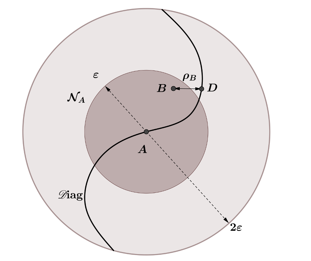
Figure 1. Cocyles $A$, $B$ and $D$ in the neighborhood $\mathscr{N}_{A}$

Proposition 3.8 of the previous section, relating the measurements $N(B)$ and $\rho(B)$, will be proved through the abstract prison break argument encapsulated in Proposition 4.3. Before specifying the sets $\Sigma_{0}$, $\Sigma_{1}$ and $\Sigma_{2}$, and for clarity, we collect below a list of constants (depending only on $A$) and conditions on the neighborhood $\mathscr{N}_{A}$ that will be needed in the argument (as well as to define the sets $\Sigma_{i}$). The following details may be skipped be at first reading.

Besides the LE $L(A)$ of $A$, let $\delta=\delta(A)$ be the size of the cones in assumption N5, let $L$ be the upper bound in assumption N3 and let $C=C(A)$ be the constant introduced above, which is $\frac{10}{9}$ of the homonymous constant in Proposition 3.5. Set the probability threshold

$$r=r(A):=\frac{L(A)}{42L(A)+60\log L}$$ (4.3)

for the application of Proposition 4.3. Let

$$M_{0}:=\frac{C\,e^{-\frac{5}{3}\,L(A)}}{1-e^{-\frac{5}{3}\,L(A)}}+\frac{C}{1-e^{-\frac{5}{3}\,L(A)}}+1,$$ (4.4)

the parameter in Lemma 4.6 below. For all $1\leq j\leq k$ set

$$\tilde{\lambda}_{j} :=e^{2\,\log\left|a_{j}\right|-\frac{L(A)}{3}},$$ (4.5)

$$\lambda^{\ast}_{j} :=e^{2\,\log\left|a_{j}\right|-\frac{L(A)}{2}}.$$ (4.6)

These families of numbers will be used to define two random walks for comparison with $\xi^{\hat{x}}_{n}(B)$, see lemmas 4.8 and 4.10 below. Next choose $s=s(A)<\infty$ such that

$$s>\max\{\,3\,(\tilde{\lambda}_{j}-\lambda_{j}^{\ast})^{-1}\colon\,1\leq j\leq k\,\},$$ (4.7)

$$s>\max\{\,(1+(\lambda_{j}^{\ast})^{-1})\,((\lambda_{j}^{\ast})^{-1}-\tilde{\lambda}_{j}^{-1})^{-1}\colon\,1\leq j\leq k\,\}.$$ (4.8)

A simple calculation gives

$$\lambda_{j}-\lambda^{\ast}_{j}\quad \leq L^{2}e^{-{L(A)\over 3}}(1-e^{-{L(A)\over 6}}),$$

$$(\lambda_{j}^{\ast})^{-1}-\tilde{\lambda}_{j}^{-1})^{-1} \leq\frac{L^{2}e^{-{L(A)\over 3}}}{e^{{L(A)\over 6}}-1}$$

and these bounds can be used to derive an explicit expression for $s(A)$. This parameter $s$ is used in lemmas 4.8 and 4.10. Define also

$$\hat{c}=\hat{c}(A):=\frac{1}{18}\,\left(\frac{L(A)}{2\log L+L(A)/2}\right)^{2}.$$ (4.9)

The parameter $\hat{c}$ will be the rate of exponential decay in Hoeffding’s inequality for the random walk determined by the numbers $\lambda^{\ast}_{j}$. Next let $l_{0}=l_{0}(A)\in\mathbb{N}$ be the smallest integer such that

$$\frac{e^{-\hat{c}\,l_{0}}}{1-e^{-\hat{c}}}<\frac{r}{8}$$ (4.10)

and let

$$\kappa=\kappa(A):=l_{0}\,\max\{-\log\lambda^{\ast}_{j}\colon 1\leq j\leq k\}.$$ (4.11)

These parameters, $\hat{c}$ and $\kappa$, appear in the proof of Proposition 4.7. Finally set

$$M=M(A) :=e^{\kappa(A)}\,s(A)\,M_{0}(A).$$ (4.12)

We now impose several assumptions that will further restrict the size of the neighborhood $\mathscr{N}_{A}$. In all statements N6-N11, $B$ is an arbitrary cocycle in $\mathscr{N}_{A}$ while $D\in\mathscr{D}{\rm iag}$ is taken, as above, near $B$. When we say that a certain assumption holds we mean that there exists a sufficiently small neighborhood $\mathscr{N}_{A}$ of $A$ such that all cocycles $B\in\mathscr{N}_{A}$ satisfy that assumption.

1. $M\,(\rho_{B})^{1\over 2}<\delta$. Holds because $\rho_{B}\leq C\,d(A,B)$ (Proposition 3.5).

2. $d(B^{-1},D^{-1})\leq C\,\rho_{B}$ and $L(D)>\frac{9}{10}\,L(A)$. The following inequality

   $$\lVert B^{-1}-D^{-1}\rVert_{\infty}\leq L^{2}\lVert B-D\rVert_{\infty}$$

   shows that if we replace $C$ by $CL^{2}$ then the first inequality holds without changing $\mathscr{N}_{A}$. Because $D$ and $A$ are diagonalizable cocycles, in view of Remark 2.2, the second assumption on $L(D)$ holds as well.

3. $\left|d_{i}\right|\geq e^{L(A)/2}$ for all $i\in\Sigma_{H}(A)$, where $D=(D_{1},\ldots,D_{k})$ and some coordinates are fixed where $D_{i}=\begin{bmatrix}d_{i}&0\\ 0&d_{i}^{-1}\end{bmatrix}$. This holds by (4.2) because $\left|a_{i}\right|\geq e^{L(A)}$.

4. $\mathscr{D}_{\pm}(D,\delta)\subset\mathscr{D}_{\pm}(A,2\delta)$. Holds because $D$ is near $A$, by (4.2).

Given $i\in\Sigma_{H}(A)$, one has $D_{i}^{\pm 1}\mathscr{D}_{\pm}(\delta)\subset\mathscr{D}_{\pm}(e^{-L(A)}\delta)$. For instance if $\hat{x}\in\mathscr{D}_{-}(\delta)$, using N8,

$$d(\hat{D}_{i}^{-1}\hat{x},\hat{e}_{-}(D)) =d(\hat{D}_{i}^{-1}\hat{x},\hat{D}_{i}^{-1}\hat{e}_{-}(D))=\frac{d(\hat{x},\hat{e}_{-}(D))}{\lVert D_{i}^{-1}x\rVert\,\lVert D_{i}^{-1}e_{-}(D)\rVert}$$

$$=\frac{d(\hat{x},\hat{e}_{-}(D))}{\lVert D_{i}^{-1}x\rVert\,\left|d_{i}\right|}\leq\delta\,\frac{d(\hat{x},\hat{e}_{+}(D))}{\lVert D_{i}^{-1}x\rVert\,\left|d_{i}\right|}$$

$$\leq\frac{\delta}{\left|d_{i}\right|^{2}}\,\frac{d(\hat{x},\hat{e}_{+}(D))}{\lVert D_{i}^{-1}x\rVert\,\left|d_{i}\right|^{-1}}\leq\frac{\delta}{\left|d_{i}\right|^{2}}\,\frac{d(\hat{x},\hat{e}_{+}(D))}{\lVert D_{i}^{-1}x\rVert\,\lVert D_{i}^{-1}e_{+}(D)\rVert}$$

$$=\frac{\delta}{e^{L(A)}}\,d(\hat{D}_{i}^{-1}\hat{x},\hat{e}_{+}(D))$$

which implies that $\hat{D}_{i}^{-1}\hat{x}\in\mathscr{D}_{-}(e^{-L(A)}\,\delta)$.

1. $\hat{B}_{i}^{\pm 1}\mathscr{D}_{\pm}(D,\delta)\subset\mathscr{D}_{\pm}(D,\delta)$ for all $i\in\Sigma_{H}(A)$. This follows by continuity from the previous considerations.

2. $\log(\rho_{B}^{-1})>\max\{2\,\kappa,l_{0}\,L(A)\}$. This holds by (4.2). Note that $\rho_{B}\searrow 0$ as the size of the neighborhood $\mathscr{N}_{A}$ decreases.

Next consider the (projective arc) sets w.r.t. the cocycle $D$

$$\Sigma_{0}:=\mathscr{D}_{-}(M\rho_{B}),\ \Sigma_{1}:=\mathscr{D}_{-}(\delta^{-1})\ \text{ and }\ \Sigma_{2}:=\mathscr{D}_{-}((M\rho_{B})^{-1}).$$

By N6, $M\,\rho_{B}<\delta$ which implies that

$$\Sigma_{0}\subset\Sigma_{1}\subset\Sigma_{2}\subset\mathbb{P}.$$

In the prisoner’s metaphor these sets are the ‘cell’, the ‘prison’ and the ‘state’. Throughout the rest of this section the projective cones $\mathscr{D}_{\pm}(a)$ always refer to the diagonal cocycle $D$.

Establishing Assumption (A1)

Proposition 4.4.

There exist constants $b_{0}>0$ and $n_{0}\in\mathbb{N}$, depending on $A$ and on the probability vector $p$, such that for all $\hat{x}\in\Sigma_{0}$,

$$\mathbb{P}_{\hat{x}}\left[\,\exists\,j\leq n_{0}\,\text{ such that }\,\xi^{\hat{x}}_{j}(B)\notin\Sigma_{0}\,\right]\geq b_{0}.$$

The proof of this proposition requires some lemmas.

Remark 4.1.

Given $g\in{\rm GL}_{2}(\mathbb{R})$ and unit vectors $x,y\in\mathbb{R}^{d}$,

$$d(\hat{g}\,\hat{x},\hat{g}\,\hat{y})=\frac{\lVert gx\wedge gy\rVert}{\lVert gx\rVert\,\lVert gy\rVert}=\frac{\left|\det g\right|\lVert x\wedge y\rVert}{\lVert gx\rVert\,\lVert gy\rVert}=\frac{\left|\det g\right|}{\lVert gx\rVert\,\lVert gy\rVert}\,d(\hat{x},\hat{y}).$$

Lemma 4.5.

Given $i\in\Sigma_{H}(A)$ for all $\hat{x},\hat{y}\in\mathscr{D}_{\pm}(\delta)$,

$$d\left(B_{i}^{\pm 1}\,\hat{x},B_{i}^{\pm 1}\,\hat{y}\right)\leq e^{-\frac{5}{3}\,L(A)}\,d(\hat{x},\hat{y}).$$

Proof.

Given $i\in\Sigma_{H}(A)$, by N5 and N9, for any $\hat{v}\in\mathscr{D}_{-}(\delta)$,

$$\lVert B_{i}\,v\rVert\leq e^{-\log\left|a_{i}\right|+\frac{L(A)}{12}}<e^{-\frac{5}{6}\,L(A)}.$$

Because of N10, we have for all $\hat{v}\in\mathscr{D}_{-}(\delta)$,

$$\lVert B_{i}^{-1}\,v\rVert>e^{\frac{5}{6}\,L(A)}\,\lVert B_{i}B_{i}^{-1}\,v\rVert\geq e^{\frac{5}{6}\,L(A)}$$

which in turn implies that for all $\hat{x},\hat{y}\in\mathscr{D}_{-}(\delta)$

$$d(\hat{B}_{i}^{-1}\,\hat{x},\hat{B}_{i}^{-1}\,\hat{y})=\frac{d(\hat{x},\hat{y})}{\lVert B_{i}^{-1}x\rVert\,\lVert B_{i}^{-1}y\rVert}\leq e^{-\frac{5}{3}\,L(A)}\,d(\hat{x},\hat{y}).$$

This proves one inequality. The other is analogous. ∎

Lemma 4.6.

For all  $1\leq j\leq k$,

$$d(\hat{B}_{j}^{\pm 1}\,\hat{e}_{\pm}(D),\hat{e}_{\pm}(D))\leq M_{0}\,\rho_{B}.$$

Proof.

Because of N10, which applies to the cocycle $A$ as well, we have $\hat{e}_{\pm}(A)\in\mathscr{D}_{\pm}(\delta)$ and $\hat{e}_{\pm}(B_{i})\in\mathscr{D}_{\pm}(\delta)$ for all $i\in\Sigma_{H}(A)$. We claim that for every $i\in\Sigma_{H}(A)$,

$$d(\hat{e}_{\pm}(B_{i}),\hat{e}_{\pm}(D))\leq\frac{C}{1-e^{-\frac{5}{3}\,L(A)}}\,\rho_{B}.$$ (4.13)

By Lemma 4.5 we have

$$d(\hat{e}_{\pm}(B_{i}),\hat{e}_{\pm}(D)) \leq d(\hat{B}_{i}^{\pm 1}\,\hat{e}_{\pm}(B_{i}),\hat{B}_{i}^{\pm 1}\,\hat{e}_{\pm}(D))+d(\hat{B}_{i}^{\pm 1}\,\hat{e}_{\pm}(D),\hat{D}_{i}^{\pm 1}\,\hat{e}_{\pm}(D))$$

$$\leq e^{-\frac{5}{3}\,L(A)}\,d(\hat{e}_{\pm}(B_{i}),\hat{e}_{\pm}(D))+\lVert B^{\pm 1}-D^{\pm 1}\rVert_{\infty},$$

which implies by N7 that

$$(1-e^{-\frac{5}{3}\,L(A)})\,d(\hat{e}_{\pm}(B_{i}),\hat{e}_{\pm}(D))\leq C\,\rho_{B}$$

and proves the claim.

Therefore, using (4.13),

$$d(\hat{B}_{j}^{\pm 1}\,\hat{e}_{\pm}(D),\hat{e}_{\pm}(D)) \leq d(\hat{B}_{j}^{\pm 1}\,\hat{e}_{\pm}(D),\hat{B}_{j}^{\pm 1}\,\hat{e}_{\pm}(B_{i}))$$

$$\quad+d(\hat{B}_{j}^{\pm 1}\,\hat{e}_{\pm}(B_{i}),\hat{e}_{\pm}(B_{i}))+d(\hat{e}_{\pm}(B_{i}),\hat{e}_{\pm}(D))$$

$$\leq e^{-\frac{5}{3}\,L(A)}\,d(\hat{e}_{\pm}(D),\hat{e}_{\pm}(B_{i}))+\rho_{B}+\frac{C}{1-e^{-\frac{5}{3}\,L(A)}}\,\rho_{B},$$

$$\leq\frac{C\,e^{-\frac{5}{3}\,L(A)}}{1-e^{-\frac{5}{3}\,L(A)}}\,\rho_{B}+\rho_{B}+\frac{C}{1-e^{-\frac{5}{3}\,L(A)}}\,\rho_{B}=M_{0}\,\rho_{B}.$$

∎

Proof of Proposition 4.4.

Fix $i\in\Sigma_{H}(A)$ and $1\leq j\leq k$ such that

$$\rho_{B}=d(\hat{B}_{j}\,\hat{e}_{-}(B_{i}),\hat{e}_{-}(B_{i})).$$

Set $b_{0}=p_{i}^{n_{0}}\,p_{j}>0$, where ${n_{0}}\in\mathbb{N}$ is large enough but yet to be chosen depending only on $A$. We claim that for any $\hat{x}\in\Sigma_{0}$ either $\hat{B}_{i}^{n_{0}}\,\hat{B}_{j}\,\hat{x}\notin\Sigma_{0}$, if $\hat{x}$ is close enough to $\hat{e}_{-}(B_{i})$, or else $\hat{B}_{i}^{n_{0}}\,\hat{x}\notin\Sigma_{0}$ otherwise. In either case the probability of these events is at least $b_{0}$.

Next we need to explain how to fix ${n_{0}}\in\mathbb{N}$, depending on $A$, so that one of the above alternative claims holds.

Given $\hat{x}\in\Sigma_{0}$, the condition $d(\hat{x},\hat{e}_{-}(B_{i}))<\frac{\rho_{B}}{L^{2}+1}$ describes the first case, in which we have

$$d(\hat{B}_{j}\,\hat{x},\hat{e}_{-}(B_{i})) \geq d(\hat{B}_{j}\,\hat{e}_{-}(B_{i}),\hat{e}_{-}(B_{i}))-d(\hat{B}_{j}\,\hat{e}_{-}(B_{i}),\hat{B}_{j}\,\hat{x})$$

$$\geq\rho_{B}-L^{2}\,d(\hat{e}_{-}(B_{i}),\hat{x})\geq\rho_{B}-L^{2}\,\frac{\rho_{B}}{L^{2}+1}=\frac{\rho_{B}}{L^{2}+1}.$$

Note that by N3 and Remark 4.1, $d(\hat{B}_{j}\,\hat{x},\hat{B}_{j}\,\hat{y})\leq L^{2}\,d(\hat{x},\hat{y})$ for all $\hat{x},\hat{y}\in\mathbb{P}$. The previous inequality shows that for any $\hat{x}\in\Sigma_{0}$, either $d(\hat{x},\hat{e}_{-}(B_{i}))\geq\frac{\rho_{B}}{L^{2}+1}$ or else $d(\hat{B}_{j}\,\hat{x},\hat{e}_{-}(B_{i}))\geq\frac{\rho_{B}}{L^{2}+1}$ and hence reduces the proof to the first case. Assuming $d(\hat{x},\hat{e}_{-}(B_{i}))\geq\frac{\rho_{B}}{L^{2}+1}$ we have to find ${n_{0}}\in\mathbb{N}$ such that

$$d(\hat{B}_{i}^{n_{0}}\,\hat{x},\hat{e}_{-}(B_{i}))\geq M^{\prime}\,\rho_{B}$$ (4.14)

with $M^{\prime}:=M+\frac{C}{1-e^{-\frac{5}{3}\,L(A)}}$. Using (4.13) this implies

$$\frac{d(\hat{B}_{i}^{n_{0}}\,\hat{x},\hat{e}_{-}(D))}{d(\hat{B}_{i}^{n_{0}}\,\hat{x},\hat{e}_{+}(D))} \geq d(\hat{B}_{i}^{n_{0}}\,\hat{x},\hat{e}_{-}(D))\geq d(\hat{B}_{i}^{n_{0}}\,\hat{x},\hat{e}_{-}(B_{i}))-d(\hat{e}_{-}(B_{i}),\hat{e}_{-}(D))$$

$$\geq M^{\prime}\,\rho_{B}-\frac{C}{1-e^{-\frac{5}{3}\,L(A)}}\,\rho_{B}=M\,\rho_{B}$$

thus proving that $\hat{B}_{i}^{n_{0}}\,\hat{x}\notin\Sigma_{0}$.

To finish, we find ${n_{0}}\in\mathbb{N}$ such that (4.14) holds. Since by N6 $\Sigma_{0}\subset\mathscr{D}_{-}(\delta)$, using Lemma 4.5 we have that

$$d(\hat{B}_{i}^{n_{0}}\,\hat{x},\hat{e}_{-}(B_{i}))\geq e^{\frac{5\,{n_{0}}}{3}\,L(A)}\,d(\hat{x},\hat{e}_{-}(B_{i}))\geq e^{\frac{5\,{n_{0}}}{3}\,L(A)}\,\frac{\rho_{B}}{L^{2}+1}\geq M^{\prime}\,\rho_{B}$$

provided we take ${n_{0}}>\frac{3}{5}\,\frac{\log[M^{\prime}\,(L^{2}+1)]}{L(A)}$. Thus we can pick ${n_{0}}\in\mathbb{N}$ depending only on $A$ such that (4.14) holds whenever $d(\hat{x},\hat{e}_{-}(B_{i}))\geq\frac{\rho_{B}}{L^{2}+1}$. ∎

Establishing Assumption (A2)

Proposition 4.7.

If $n_{1}(B):=\lceil\frac{2}{L(A)}\,\log(\rho_{B}^{-1})\rceil$ then for all $\hat{x}\in\Sigma_{1}\setminus\Sigma_{0}$,

$$\mathbb{P}_{\hat{x}}\left[\,\exists\,j\leq n_{1}\,,\;\xi^{\hat{x}}_{j}(B)\notin\Sigma_{1}\,\right]\geq 1-r/4.$$

Consider the projective coordinate system $\psi=\psi_{-}$ introduced above, in which $\hat{e}_{-}(D)=0$ and $\hat{e}_{+}(D)=\infty$.

We will keep denoting by $\hat{B}_{j}$ the action of $B_{j}$ expressed in the previous projective coordinate, i.e., we write $\hat{B}_{j}(x):=\psi(\hat{B}_{j}(x:1))$. Consider the family of numbers $\{\lambda^{\ast}_{j}\}_{1\leq j\leq k}$ defined in (4.6). A simple calculation gives

$$\sum_{j=1}^{k}p_{j}\,\log\lambda^{\ast}_{j}=\frac{3\,L(A)}{2}>0.$$ (4.15)

Lemma 4.8.

For all $x\in[s\,M_{0}\,\rho_{B},\delta^{-1}]$ and $1\leq j\leq k$,

$$\hat{B}_{j}(x)\geq M_{0}\,\rho_{B}+\lambda^{\ast}_{j}\,(x-M_{0}\,\rho_{B})=:\hat{B}_{j}^{\ast}(x).$$ (4.16)

Proof.

By Lemma 4.6, the projective point $\hat{B}_{j}(\hat{e}_{-}(D))$ has coordinate $|\hat{B}_{j}(0)|\leq 2\,M_{0}\,\rho_{B}$.

Writing $B_{j}=\begin{bmatrix}b_{j}&c_{j}\\ d_{j}&e_{j}\end{bmatrix}$ one has $\hat{B}_{j}(x)=(b_{j}\,x+c_{j})\,(d_{j}\,x+e_{j})^{-1}$. Since $B_{j}\in{\rm SL}_{2}(\mathbb{R})$, $\left|d_{j}\right|\leq\lVert B-D\rVert_{\infty}<d(A,B)$ and $0\leq x\leq\delta^{-1}$ we have

$$\hat{B}_{j}^{\prime}(x)=\frac{1}{(d_{j}\,x+e_{j})^{2}}\geq\frac{1}{(\left|e_{j}\right|+\delta^{-1}\,d(A,B))^{2}}.$$

Because $\hat{e}_{\pm}(A)\in\mathscr{D}_{\pm}(\delta)$, by N10, and also by N5 and N9,

$$\left|e_{j}\right|\leq\lVert B_{j}\,e_{-}(D)\rVert\leq e^{-\log\left|a_{j}\right|+\frac{L(A)}{12}}=\tilde{\lambda}_{j}^{-\frac{1}{2}}\,e^{-\frac{L(A)}{12}}<\tilde{\lambda}_{j}^{-\frac{1}{2}}.$$

Thus for all $j=1,\ldots,k$ and $x\in[0,\delta^{-1}]$,

$$\hat{B}_{j}^{\prime}(x)\geq\frac{1}{(\tilde{\lambda}_{j}^{-\frac{1}{2}}e^{-\frac{L(A)}{12}}+\delta^{-1}d(A,B))^{2}}\geq\frac{\tilde{\lambda}_{j}\,e^{\frac{L(A)}{6}}}{(1+\delta^{-1}Le^{\frac{L(A)}{4}}d(A,B))^{2}}.$$

By N0 (a)

$$d(A,B)<\frac{\delta}{L}\,\frac{e^{\frac{L(A)}{12}}-1}{e^{\frac{L(A)}{4}}}$$

which is equivalent to

$$\gamma=\frac{e^{\frac{L(A)}{6}}}{(1+\delta^{-1}Le^{\frac{L(A)}{4}}d(A,B))^{2}}>1.$$

Therefore $\hat{B}_{j}^{\prime}(x)\geq\gamma\,\tilde{\lambda}_{j}>\tilde{\lambda}_{j}$ and by the mean value theorem for all $0\leq x\leq\delta^{-1}$,

$$\hat{B}_{j}(x)\geq\hat{B}_{j}(0)+\tilde{\lambda}_{j}\,x\geq-2\,M_{0}\,\rho_{B}+\tilde{\lambda}_{j}\,x.$$

Since $\hat{B}_{j}^{\prime}(x)\geq\tilde{\lambda}_{j}>\lambda^{\ast}_{j}=(\hat{B}^{\ast}_{j})^{\prime}(x)$, to see that $\hat{B}_{j}(x)\geq\hat{B}^{\ast}_{j}(x)$ for all $x\in[s\,M_{0}\,\rho_{B},\delta^{-1}]$, it is now enough to check that

$$-2\,M_{0}\,\rho_{B}+\tilde{\lambda}_{j}\,(s\,M_{0}\,\rho_{B}) \geq\hat{B}^{\ast}_{j}(s\,M_{0}\,\rho_{B})$$

$$=M_{0}\,\rho_{B}+\lambda^{\ast}_{j}\,(s\,M_{0}\,\rho_{B}-M_{0}\,\rho_{B}),$$

which is equivalent to

$$-2+\tilde{\lambda}_{j}\,s\geq 1+\lambda^{\ast}_{j}\,(s-1).$$

Hence, because (4.7) is enough for this, by the definition of $s=s(A)$ inequality (4.16) holds for all $x\in[s\,M_{0}\,\rho_{B},\delta^{-1}]$. ∎

Consider the i.i.d. process $\eta_{n}\colon X\to\mathbb{R}_{+}$, $\eta_{n}\{\omega_{j}\}_{j\in\mathbb{Z}}:=\log\lambda^{\ast}_{\omega_{j}}$ and its associated sum process $S_{n}=\sum_{j=0}^{n-1}\eta_{j}=\sum_{j=0}^{n-1}\eta_{0}\circ T^{j}$. Note that the processes $\{\eta_{n}\}$ and $\{S_{n}\}$ are completely determined by the cocycle $A$.

The probability of escaping in assumption (A2) is estimated comparing the random walks $\xi^{\hat{x}}_{n}$ and $S_{n}$ by means of (4.16).

Proof of Proposition 4.7.

By (4.15) one has $\mathbb{E}[\eta_{0}]=\frac{3\,L(A)}{2}$. By Hoeffding’s inequality (Lemma 2.2) the constant $\hat{c}=\hat{c}(A)$ in (4.9) is such that the following LDT estimate holds for all $n\in\mathbb{N}$,

$$\mathbb{P}_{p}[\,S_{n}<n\,L(A)\,]<e^{-\hat{c}\,n}.$$ (4.17)

Indeed the i.i.d. process $\eta_{j}$ satisfies

$$\left|\eta_{j}\right|=\left|\log\lambda^{\ast}_{\omega_{j}}\right|=\left|2\,\log\left|a_{\omega_{j}}\right|-L(A)/2\right|\leq 2\log L+L(A)/2=:K$$

while the event $[S_{n}<nL(A)]$ is contained in the deviation set

$$\left[\,\bigl{|}\ n^{-1}S_{n}-\mathbb{E}(n^{-1}S_{n})\bigr{|}>\epsilon\,\right]\quad\text{ with }\quad\epsilon:=\frac{L(A)}{3}.$$

Since $\hat{c}=\frac{\epsilon^{2}}{2K^{2}}$, the previous LDT estimate follows from Hoeffding’s inequality.

Consider now $l_{0}\in\mathbb{N}$ and $\kappa<\infty$ respectively defined by (4.10) and in (4.11). Then   $\sum_{j=l_{0}}^{\infty}e^{-\hat{c}\,j}=\frac{e^{-\hat{c}l_{0}}}{1-e^{-\hat{c}}}<\frac{r}{8}$   and

$$\mathbb{P}_{p}[\,S_{j}\geq-\kappa,\;\forall\,j=1,\ldots,l_{0}\,]=1.$$ (4.18)

This implies that the event $\Omega=[\,S_{j}\geq-\kappa,\;\forall\,j\geq 1\,]$ has probability $\mathbb{P}_{p}(\Omega)\geq 1-\frac{r}{8}$.

Given $\hat{x}\in\Sigma_{1}\setminus\Sigma_{0}$, we have $t=\left|\psi(\hat{x})\right|\in[M\,\rho_{B},\delta^{-1}]$. Inductively, and while $\xi^{\hat{x}}_{n}\in\Sigma_{1}$, one obtains by successive applications of inequality (4.16) that for all $\omega=\{\omega_{j}\}_{j\in\mathbb{Z}}\in\Omega$,

$$\left|\psi(\xi^{\hat{x}}_{n}(\omega))\right| =\hat{B}_{\omega_{n-1}}\,\ldots\,\hat{B}_{\omega_{1}}\,\hat{B}_{\omega_{0}}(t)\geq B^{\ast}_{\omega_{n-1}}\,\ldots\,\hat{B}^{\ast}_{\omega_{1}}\,\hat{B}^{\ast}_{\omega_{0}}(t)$$

$$\geq M_{0}\,\rho_{B}+e^{S_{n}}\,(t-M_{0}\,\rho_{B})$$

$$\geq e^{-\kappa}\,M\,\rho_{B}=s\,M_{0}\,\rho_{B}$$

which in particular justifies that we can keep inductively applying inequality (4.16).

Consider now the event $\mathscr{B}=[\,S_{n_{1}}<n_{1}\,L(A)\,]$ which by (4.17) has probability $<e^{-\hat{c}\,n_{1}}$. By N11, $l_{0}<n_{1}$ and by (4.10), $e^{-\hat{c}\,l_{0}}<\frac{r}{8}$. Then the event $\Omega^{\prime}=\Omega\setminus\mathscr{B}$ has probability

$$\mathbb{P}_{p}(\Omega^{\prime})\geq\mathbb{P}_{p}(\Omega)-\mathbb{P}_{p}(\mathscr{B})\geq 1-\frac{r}{8}-e^{-\hat{c}\,n_{1}}>1-\frac{r}{4}.$$

Assume now, by contradiction, that for some $\omega\in\Omega^{\prime}$ one has for all $j\leq n_{1}$, $\xi^{\hat{x}}_{n}=\xi^{\hat{x}}_{n}(\omega)\in\Sigma_{1}$. This implies that $\left|\psi(\xi^{\hat{x}}_{j})\right|\in[M\,\rho_{B},\delta^{-1}]$ for all $j\leq n_{1}$. We can assume that the number $s=s(A)$ defined by (4.7) and (4.8) satisfies $s\geq 2$. Because $M_{0}\geq 1$, it follows that $M\geq M_{0}+1$. Then the previous inductive chain of inequalities implies that

$$\left|\psi(\xi^{\hat{x}}_{n_{1}})\right| \geq M_{0}\,\rho_{B}+e^{S_{n_{1}}}\,(t-M_{0}\,\rho_{B})$$

$$\geq e^{{n_{1}}\,L(A)}\,(t-M_{0}\,\rho_{B})\geq e^{{n_{1}}\,L(A)}\,(M-M_{0})\,\rho_{B}$$

$$\geq e^{{n_{1}}\,L(A)}\,\rho_{B}=\frac{1}{\rho_{B}^{2}}\,\rho_{B}=\rho_{B}^{-1}>\delta^{-1},$$

which contradicts $\xi^{\hat{x}}_{n_{1}}\in\Sigma_{1}$. This concludes the proof. ∎

Establishing Assumption (A3)

Proposition 4.9.

If $n_{2}(B):=\lceil\frac{1}{L(A)}\,\log(\rho_{B}^{-1})\rceil$ then for all $\hat{x}\in\Sigma_{2}\setminus\Sigma_{1}$,

$$\mathbb{P}_{\hat{x}}\left[\,\exists\,j\leq n_{2}\,,\;\xi^{\hat{x}}_{j}\notin\Sigma_{2}\,\right]\geq 1-r/4.$$

Consider the projective coordinate system $\psi=\psi_{+}$ introduced above, in which $\Sigma_{1}^{\complement}=\mathscr{D}_{-}(\delta^{-1})^{\complement}=[-\delta,\delta]$ and $\Sigma_{2}^{\complement}=\mathscr{D}_{-}((M\rho_{B})^{-1})^{\complement}=[-M\rho_{B},M\rho_{B}]$.

We will keep denoting by $\hat{B}_{j}$ the action of $B_{j}$ expressed in the previous projective coordinate, i.e., we write $\hat{B}_{j}(x):=\psi(\hat{B}_{j}(1:x))$.

Consider again the parameters $\tilde{\lambda}_{j}$, $\lambda_{j}^{\ast}$ defined in (4.5) and  (4.6).

Lemma 4.10.

For all $x\in[s\,M_{0}\,\rho_{B},\,(e^{\kappa}+1)\,\delta]$ and $1\leq j\leq k$,

$$\hat{B}_{j}(x)\leq M_{0}\,\rho_{B}+(\lambda^{\ast}_{j})^{-1}\,(x-M_{0}\,\rho_{B})=:\hat{B}_{j}^{\ast}(x).$$ (4.19)

Proof.

By Lemma 4.6, the projective point $\hat{B}_{j}(\hat{e}_{+}(D))$ has coordinate $|\hat{B}_{j}(0)|\leq 2\,M_{0}\,\rho_{B}$.

Writing $B_{j}=\begin{bmatrix}b_{j}&c_{j}\\ d_{j}&e_{j}\end{bmatrix}$ one has $\hat{B}_{j}(x)=(d_{j}+e_{j}\,x)\,(b_{j}+c_{j}\,x)^{-1}$. Since $B_{j}\in{\rm SL}_{2}(\mathbb{R})$, $\left|c_{j}\right|\leq\lVert B-D\rVert_{\infty}<d(A,B)$ and $0\leq x\leq\delta^{-1}$ we have

$$\hat{B}_{j}^{\prime}(x)=\frac{1}{(b_{j}+c_{j}\,x)^{2}}\leq\frac{1}{(\left|b_{j}\right|-\delta^{-1}\,d(A,B))^{2}}.$$

Because $\left|d_{j}\right|\leq d(A,B)$ and $\left|b_{j}\right|\geq\left|a_{j}\right|-d(A,B)\geq L^{-1}-d(A,B)$,

$$\frac{\left|b_{j}\right|}{\sqrt{b_{j}^{2}+d_{j}^{2}}}=\frac{1}{\sqrt{1+\frac{d_{j}^{2}}{b_{j}^{2}}}}>\frac{1}{\sqrt{1+\frac{d(A,B)^{2}}{(L^{-1}-d(A,B))^{2}}}}>e^{-\frac{L(A)}{24}},$$

where the last inequality follows from N0(b). Therefore

$$\left|b_{j}\right| \geq e^{-\frac{L(A)}{24}}\,\sqrt{b_{j}^{2}+d_{j}^{2}}=e^{-\frac{L(A)}{24}}\lVert B_{j}\,e_{+}(D)\rVert$$

$$\geq e^{-\frac{L(A)}{24}}\,e^{\log\left|a_{j}\right|-\frac{L(A)}{12}}=\tilde{\lambda}_{j}^{\frac{1}{2}}\,e^{\frac{L(A)}{24}}>\tilde{\lambda}_{j}^{\frac{1}{2}}.$$

Thus for all $j=1,\ldots,k$ and $x\in[0,\delta^{-1}]$,

$$\hat{B}_{j}^{\prime}(x)\leq\frac{1}{(\tilde{\lambda}_{j}^{\frac{1}{2}}e^{\frac{L(A)}{24}}-\delta^{-1}d(A,B))^{2}}\leq\frac{\tilde{\lambda}_{j}^{-1}\,e^{-\frac{L(A)}{12}}}{(1-\delta^{-1}Le^{\frac{L(A)}{8}}d(A,B))^{2}}.$$

By N0 (c)

$$d(A,B)<\delta\,L^{-1}\,{e^{-\frac{L(A)}{8}}}\,\left(1-e^{-\frac{L(A)}{24}}\right)$$

which is equivalent to

$$\gamma=\frac{e^{-\frac{L(A)}{12}}}{(1-\delta^{-1}Le^{\frac{L(A)}{8}}d(A,B))^{2}}<1.$$

Therefore $\hat{B}_{j}^{\prime}(x)\leq\gamma\,\tilde{\lambda}_{j}^{-1}<\tilde{\lambda}_{j}^{-1}$ and by the mean value theorem for all $0\leq x\leq\delta^{-1}$,

$$\hat{B}_{j}(x)\leq\hat{B}_{j}(0)+\tilde{\lambda}_{j}^{-1}\,x\leq 2\,M_{0}\,\rho_{B}+\tilde{\lambda}_{j}^{-1}\,x.$$

Since $\hat{B}_{j}^{\prime}(x)\leq\tilde{\lambda}_{j}^{-1}<(\lambda^{\ast}_{j})^{-1}=(\hat{B}^{\ast}_{j})^{\prime}(x)$, inequality $\hat{B}_{j}(x)\leq\hat{B}^{\ast}_{j}(x)$, for all $x\in[s\,M_{0}\,\rho_{B},\delta^{-1}]$, follows from

$$2\,M_{0}\,\rho_{B}+\tilde{\lambda}_{j}^{-1}\,(s\,M_{0}\,\rho_{B}) \leq\hat{B}^{\ast}_{j}(s\,M_{0}\,\rho_{B})$$

$$=M_{0}\,\rho_{B}+(\lambda^{\ast}_{j})^{-1}\,(s\,M_{0}\,\rho_{B}-M_{0}\,\rho_{B}),$$

which is equivalent to

$$2+\tilde{\lambda}_{j}^{-1}\,s \leq 1+(\lambda^{\ast}_{j})^{-1}\,(s-1).$$

Hence, because (4.8) is enough for this, by the definition of $s=s(A)$, inequality (4.19) holds for all $x\in[s\,M_{0}\,\rho_{B},\delta^{-1}]$. Finally, because $\delta$ can be made small enough we may assume that $(e^{\kappa}+1)\,\delta<\delta^{-1}$. ∎

The probability of escaping in assumption (A3) is estimated comparing again the random walks $\xi^{\hat{x}}_{n}$ and $S_{n}$, now by means of (4.19). The argument is analogous to the one used for assumption (A2).

Proof of Proposition 4.9.

Consider the constants $\hat{c}=\hat{c}(A)>0$, $l_{0}=l_{0}(A)$ and $\kappa=\kappa(A)<\infty$, respectively defined in (4.9), (4.10) and (4.11) and consider the event

$$\Omega^{\prime}=[\,S_{n_{2}}>n_{2}\,L(A)\,\text{ and }\;S_{j}\geq-\kappa,\;\forall\,j\geq 1\,]$$

which, as we have seen in the proof of Proposition 4.7, has probability $\mathbb{P}_{p}(\Omega)\geq 1-\frac{r}{4}$.

Given $\hat{x}\in\Sigma_{2}\setminus\Sigma_{1}$, we have $t=\left|\psi(\hat{x})\right|\in[M\,\rho_{B},\delta]$. Inductively, and while $\xi^{\hat{x}}_{n}\in\Sigma_{2}$, one obtains by successive applications of inequality (4.19) that for all $\omega=\{\omega_{j}\}_{j\in\mathbb{Z}}\in\Omega^{\prime}$,

$$\left|\psi(\xi^{\hat{x}}_{n}(\omega))\right| =\hat{B}_{\omega_{n-1}}\,\ldots\,\hat{B}_{\omega_{1}}\,\hat{B}_{\omega_{0}}(t)\leq B^{\ast}_{\omega_{n-1}}\,\ldots\,\hat{B}^{\ast}_{\omega_{1}}\,\hat{B}^{\ast}_{\omega_{0}}(t)$$

$$\leq M_{0}\,\rho_{B}+e^{-S_{n}}\,(t-M_{0}\,\rho_{B})$$

$$\leq M_{0}\,\rho_{B}+e^{\kappa}\,\delta<\delta\,(e^{\kappa}+1)$$

which in particular justifies that we can keep inductively applying (4.19). The last inequality above follows from N6.

Assume now, by contradiction, that for some $\omega\in\Omega^{\prime}$ one has for all $j\leq n_{2}$, $\xi^{\hat{x}}_{n}=\xi^{\hat{x}}_{n}(\omega)\in\Sigma_{2}$. This implies that $\left|\psi(\xi^{\hat{x}}_{j})\right|\in[M\,\rho_{B},\delta]$ for all $j\leq n_{2}$. Because $M_{0}+\delta<M_{0}+1<M$, the previous inductive chain of inequalities implies that

$$\left|\psi(\xi^{\hat{x}}_{n_{2}})\right| \leq M_{0}\,\rho_{B}+e^{-S_{n_{2}}}\,(t-M_{0}\,\rho_{B})$$

$$\leq M_{0}\,\rho_{B}+e^{-{n_{2}}\,L(A)}\,(t-M_{0}\,\rho_{B})\leq M_{0}\,\rho_{B}+e^{-{n_{2}}\,L(A)}\,\delta$$

$$\leq M_{0}\,\rho_{B}+\rho_{B}\,\delta<M\,\rho_{B},$$

which contradicts $\xi^{\hat{x}}_{n_{1}}\in\Sigma_{2}$. This concludes the proof. ∎

Establishing Assumption (A4)

Proposition 4.11.

For all $\hat{x}\in\Sigma_{2}^{\complement}$,

$$\mathbb{P}_{\hat{x}}\left[\,\forall\,j\geq 0\,,\;\xi^{\hat{x}}_{j}(B)\notin\Sigma_{1}\,\right]\geq 1-r/4.$$

Proof.

Consider the projective coordinate $\psi=\psi_{+}$ introduced in the previous subsection. Through this coordinate system we make the identifications $\Sigma_{2}^{\complement}\equiv\mathscr{D}_{-}((M\,\rho_{B})^{-1})^{\complement}=[-M\,\rho_{B},M\,\rho_{B}]$ and $\Sigma_{1}^{\complement}\equiv\mathscr{D}_{-}(\delta)^{\complement}=[-\delta,\delta]$.

Given $\hat{x}\in\Sigma_{2}^{\complement}$ and $N\in\mathbb{N}$, consider the event

$$\Omega_{N}:=[\,\exists\,1\leq j\leq N\,\text{ such that }\,\xi^{\hat{x}}_{j}\in\Sigma_{1}\,].$$

Our goal is to prove that $\mathbb{P}(\Omega_{N})<r/4$  for all $N\in\mathbb{N}$.

Consider the following family of events indexed in $0\leq i\leq N$

$$\mathscr{E}^{N}_{i}:=\left[\,\xi^{\hat{x}}_{i}\notin\Sigma_{2}\,\text{ and }\,\forall\,i<l\leq N,\;\xi^{\hat{x}}_{l}\in\Sigma_{2}\,\right].$$

Because $\hat{x}\notin\Sigma_{2}$, these events partition the space of sequences $X$.

As before, let $S_{n}:=\sum_{j=0}^{n-1}\eta\circ T^{j}$ be the sum process associated with the i.i.d. process generated by the random variable $\eta\colon X\to\mathbb{R}$, $\eta(\omega):=\log\lambda_{\omega_{0}}^{\ast}$. Given $\omega\in\Omega_{N}\cap\mathscr{E}^{N}_{i}$, let $t_{i}:=\left|\psi(\xi^{\hat{x}}_{i}(\omega))\right|<M\,\rho_{B}$ and $n\in[1,N-i]$ be the first integer such that $\xi^{\hat{x}}_{i+n}\in\Sigma_{1}$. Proceeding inductively, from inequality (4.19) we get that

$$\delta\leq\left|\psi(\xi^{\hat{x}}_{i+n}(\omega))\right| =\hat{B}_{\omega_{i+n-1}}\,\ldots\,B_{\omega_{i+1}}\,B_{\omega_{i}}(t_{i})\leq\hat{B}_{\omega_{\tilde{\i}+n-1}}^{\ast}\,\ldots\,B_{\omega_{i+1}}^{\ast}\,B_{\omega_{i}}^{\ast}(t_{i})$$

$$\leq M_{0}\,\rho_{B}+e^{-S_{n}(T^{i}\omega)}\,(t_{i}-M_{0}\,\rho_{B})$$

$$<M_{0}\,\rho_{B}+e^{-S_{n}(T^{i}\omega)}\,(M-M_{0})\,\rho_{B}.$$

By N6 this implies that $e^{-S_{n}(T^{i}\omega)}>1$ and hence that

$$\delta<e^{-S_{n}(T^{i}\omega)}\,M\,\rho_{B}.$$

In other words we have established the inclusion

$$\Omega_{N}\cap\mathscr{E}^{N}_{i}\subset T^{-i}\left[\,\exists\,n\geq 1\,\text{ such that }\,e^{-S_{n}}\,M\,\rho_{B}>\delta\,\right],$$

which implies that

$$\mathbb{P}[\,\Omega_{N}\,|\,\mathscr{E}^{N}_{i}\,]\leq\mathbb{P}\left[\,\exists\,n\geq 1\,\text{ such that }\,e^{-S_{n}}\,M\,\rho_{B}>\delta\,\right].$$

Next, define $l=l(A):=\max\{\log(\lambda_{j}^{\ast})^{-1}\colon 1\leq j\leq k\}$ so that $S_{n}\geq-n\,l$ for all $n\geq 0$. Note also that $l=\kappa/l_{0}>0$. By assumption N6 we have $M\,\rho_{B}^{1/2}<\delta$. Since

$$e^{-S_{n}}\,M\,\rho_{B}>\delta\quad \Leftrightarrow\quad e^{S_{n}}<\delta^{-1}\,M\,\rho_{B}<\rho_{B}^{1/2}$$

$$\Rightarrow\quad-n\,l\leq S_{n}<\frac{1}{2}\,\log(\rho_{B})<0$$

$$\Rightarrow\quad n\geq\frac{1}{2\,l}\,\log(\rho_{B}^{-1})\;\text{ and }\;S_{n}<n\,L(A).$$

it follows that

$$\mathbb{P}[\,\Omega_{N}\,|\,\mathscr{E}^{N}_{i}\,]\leq\mathbb{P}[\;\exists\,n\geq\frac{1}{2\,l}\,\log(\rho_{B}^{-1})\;\text{ such that }\;S_{n}<n\,L(A)\;]$$

which by (4.17),  (4.10) and assumption N11 has probability

$$\frac{e^{-\frac{\hat{c}}{2\,l}\,\log(\rho_{B}^{-1})}}{1-e^{-\hat{c}}}=\frac{e^{-\frac{\hat{c}\,l_{0}}{2\,\kappa}\,\log(\rho_{B}^{-1})}}{1-e^{-\hat{c}}}<\frac{e^{-\hat{c}\,l_{0}}}{1-e^{-\hat{c}}}<\frac{r}{8}<\frac{r}{4}.$$

Finally, applying the Law of Total Probabilities

$$\mathbb{P}(\Omega_{N}) =\sum_{i=0}^{n-1}\mathbb{P}[\,\Omega_{N}\,|\,\mathscr{E}^{N}_{i}\,]\,\mathbb{P}(\mathscr{E}^{N}_{i})$$

$$<\frac{r}{4}\,\sum_{i=0}^{n-1}\mathbb{P}(\mathscr{E}^{N}_{i})=\frac{r}{4}.$$

∎

Conclusion

We now apply the general prison break result to our setting.

Proposition 4.12.

Let $A\in\mathcal{C}$ be a diagonalizable cocycle such that $L(A)>0$. There exists $c_{0}=c_{0}(A)<\infty$ such that if $B\in\mathscr{N}_{A}$ with $\rho_{B}=\rho_{-}(B)>0$ and $n_{B}:=c_{0}\,\log(\rho_{B}^{-1})$ then for all $\hat{x}\in\mathbb{P}$

$$\mathbb{P}\left[\,\exists j\geq n_{B},\quad\xi^{\hat{x}}_{j}(B)\in\Sigma_{1}\;\right]<r.$$ (4.20)

Proof.

Take ${n_{0}}\in\mathbb{N}$ and $b_{0}>0$ as given by Proposition 4.4. Next choose $q=q(A)\in\mathbb{N}$ such that $q\geq\frac{1}{b_{0}}\,\log(4/r)$, which implies that $(1-b_{0})^{q}<\frac{r}{4}$. Take $n_{1}=n_{1}(B)$ and $n_{2}=n_{2}(B)\in\mathbb{N}$ as given by propositions 4.7 and 4.9.

By Proposition 4.11, $\mathbb{P}_{\hat{x}}\left[\,\forall\,j\geq 0\,,\;\xi^{\hat{x}}_{j}\notin\Sigma_{1}\,\right]\geq 1-r/4$, for all $\hat{x}\in\Sigma_{2}^{\complement}$.

Therefore all assumptions (A1)-(A4) of Proposition 4.3 are satisfied, the first three within the times $n_{0}$, $n_{1}$ and $n_{2}$ respectively. Reducing the neighborhood $\mathscr{N}_{A}$ we can assume that $\log\rho_{B}^{-1}>n_{0}$ for all $B\in\mathscr{N}_{A}$. Since the time $N=q\,n_{0}+n_{1}+n_{2}$ is bounded above by $c_{0}\,\log(\rho_{B}^{-1})$ with $c_{0}=q+\frac{3}{L(A)}$, $c_{0}$ being a constant depending only on $A$, the conclusion of this proposition follows from that of Proposition 4.3. ∎

Proof of Proposition 3.8.

The second inequality reduces to applying the first one to the inverse cocycle $B^{-1}$. Thus, from now on we will focus on the first.

Since $A\in\mathscr{D}{\rm iag}^{\ast}$ we may assume without loss of generality that $A$ is a diagonal cocycle,

$$A_{i}=\begin{bmatrix}a_{i}&0\\ 0&a_{i}^{-1}\end{bmatrix}\qquad\text{ for }\;1\leq i\leq k$$

and so $\hat{e}_{+}(A)=(1:0)$ and $\hat{e}_{-}(A)=(0:1)$. In the coordinate system $\psi_{+}$ associated with the diagonal cocycle $A$, the projective action of the matrix $A_{i}$ is given by $\hat{A}_{i}\,x=a_{i}^{-2}\,x$. In these coordinates, the random walk $\xi_{n}^{\hat{v}}=\xi_{n}^{\hat{v}}(A)$ becomes a random walk $\xi^{x}_{n}$ on the real line with starting point $x$, where $\hat{v}=(1\colon x)$.

Next consider the i.i.d. process $\eta_{n}$, where $\eta_{n}=\log\left|a_{i}\right|$ with probability $p_{i}$, and denote by $S_{n}=\sum_{j=0}^{n-1}\eta_{j}$ the corresponding sum process. A simple verification shows that

$$\mathbb{E}[\frac{1}{n}\,S_{n}]=\mathbb{E}[\eta_{0}]=L(A).$$

By Hoeffding’s inequality there exist positive constants $n_{0}\in\mathbb{N}$ and $c_{1}$ depending only on $A$ such that for all $n\geq n_{0}$,

$$\mathbb{P}\left[\,\exists j\geq n,\;\frac{1}{j}\,S_{j}<\frac{9}{10}\,L(A)\,\right]<e^{-c_{1}\,n}.$$ (4.21)

Let $c_{0}=c_{0}(A)$ and $n_{B}=c_{0}\,\log\rho_{B}^{-1}$ be the constants provided by Proposition 4.12. Making $\mathscr{N}_{A}$ small enough, since by Proposition 3.5 $\rho_{B}\lesssim d(A,B)$, we can assume that $n_{B}\geq n_{0}$. Then take the union $\mathscr{B}=\mathscr{B}_{1}\cup\mathscr{B}_{2}$ of the sets defined in (4.20) and (4.21), i.e.,

$$\mathscr{B}_{1} :=\left\{\omega\in X\colon\exists j\geq n_{B}\quad\xi^{\hat{x}}_{j}(B)(\omega)\in\Sigma_{1}\right\},$$

$$\mathscr{B}_{2} :=\left\{\omega\in X\colon\frac{1}{n}\,S_{n}(\omega)<\frac{9}{10}\,L(A)\,\text{ for some }\,n\geq n_{B}\right\}.$$

For each matrix $B_{j}$ consider the projective function $\varphi_{B_{j}}(\hat{v}):=\log\lVert B_{j}\,v\rVert$. By N5 and N9, for all $\hat{v}\in\mathscr{D}_{+}(A,2\delta)$ and $1\leq j\leq k$

$$\bigl{|}\varphi_{B_{j}}(\hat{v})-\log\left|a_{j}\right|\bigr{|}=\bigl{|}\log\lVert B_{j}v\rVert-\log\lVert A_{j}\,e_{+}(A)\rVert\bigr{|}\leq\frac{L(A)}{12}.$$

Given $\omega=\{\omega_{j}\}_{j\in\mathbb{Z}}\notin\mathscr{B}$ and $\hat{v}\in\mathbb{P}$, because $\xi^{\hat{v}}_{j}(B)\in\Sigma_{1}^{\complement}=\overline{\mathscr{D}_{+}(\delta)}\subset\mathscr{D}_{+}(A,2\delta)$ for all $n\geq n_{B}$,

$$\bigl{|}\frac{1}{n}\,\log\lVert B^{(n)}\,v\rVert-\frac{1}{n}\,S_{n}\bigr{|} \leq\frac{1}{n}\,\sum_{j=0}^{n-1}\bigl{|}\varphi_{B_{\omega_{j}}}(\xi^{\hat{v}}_{j}(B))-\log\left|a_{\omega_{j}}\right|\bigr{|}$$

$$\leq\frac{n_{B}}{n}\,2\,\log L+\frac{n-n_{B}}{n}\,\frac{L(A)}{12}$$

$$\leq 2\,\frac{n_{B}}{n}\,\log L+\frac{L(A)}{12}\leq\frac{L(A)}{10}$$

where the last inequality holds for $n\geq\frac{120\,\log L}{L(A)}\,n_{B}$.

Hence, since $\omega\notin\mathscr{B}_{2}$ and $n\geq n_{0}$,

$$\frac{1}{n}\,\log\lVert B^{(n)}v\rVert\geq\frac{1}{n}\,S_{n}-\frac{L(A)}{10}\geq\left(\frac{9}{10}-\frac{1}{10}\right)\,L(A)>\frac{7}{10}\,L(A).$$

Therefore, integrating we have for every $\hat{v}\in\mathbb{P}$ and $n\geq\frac{120\,\log L}{L(A)}\,n_{B}$,

$$\mathbb{E}\left[\frac{1}{n}\,\log\lVert B^{(n)}v\rVert\right] \geq-(\log L)\,\mathbb{P}(\mathscr{B})+(1-\mathbb{P}(\mathscr{B}))\,\frac{7\,L(A)}{10}$$

$$\geq\frac{2\,L(A)}{3}>\frac{L(B)}{2}$$

where the last inequality holds by assumption N2, and the one next-to-last is also valid provided

$$\mathbb{P}(\mathscr{B})<\frac{L(A)}{30\,\log L+21\,L(A)}=2r.$$ (4.22)

Note from the above that in particular we also have

$$L(B)\geq\frac{2L(A)}{3}$$ (4.23)

for all $B\in\mathscr{N}_{A}$. By (4.21) and Proposition 4.12, the inequality

$$\mathbb{P}(\mathscr{B})<r+e^{-c_{1}n_{B}}<2\,r$$

is equivalent to

$$n_{B} \geq\frac{1}{c_{1}}\,\log\left(42+\frac{60\,\log L}{L(A)}\right).$$

Since the right-hand-side of this inequality depends only on $A$, reducing the neighborhood $\mathscr{N}_{A}$, we can assume that it holds for all $B\in\mathscr{N}_{A}$. Therefore, setting $K=\frac{120\,\log L}{L(A)}$, for all $n\geq K\,n_{B}$ and $\hat{v}\in\mathbb{P}$, relation  (4.22) holds which in turn implies that

$$\mathbb{E}\left[\frac{1}{n}\,\log\lVert B^{(n)}v\rVert\right]>\frac{L(B)}{2}.$$

By Definition 3.1 this proves that

$$N(B)\leq K\,n_{B}\leq K\,c_{0}\,\log(\rho_{-}(B)^{-1}).$$

The proposition is established with $c=K^{-1}\,c_{0}^{-1}$. ∎

Remark 4.2.

As a bi-product of the previous proof we derive the fact (to be used later) that $L(B)\geq 2L(A)/3$.

An improvement of this argument leads to the lower semi-continuity of the LE, which when combined with the upper-semicontinuity shows that the LE function $A\mapsto L(A)$ is continuous at any diagonalizable cocycle $A\in{\rm SL}_{2}(\mathbb{R})^{k}$ with $L(A)>0$. As remarked in [1], E. Le Page’s Theorem on the Hölder continuity of the LE holds for quasi-irreducible ${\rm SL}_{2}$-cocycles $A$ such that $L(A)>0$. For any non diagonalizable ${\rm SL}_{2}$-cocycle $A$ such that $L(A)>0$ either $A$ or else the inverse cocycle $A^{-1}$ are quasi-irreducible. Finally, since the continuity of the LE at $A$ is equivalent to the continuity at $A^{-1}$, combining these facts we get an alternative proof of C. Boker-Neto and M. Viana’s Theorem [2] on the general continuity of the LE for ${\rm SL}_{2}(\mathbb{R})$ and ${\rm GL}_{2}(\mathbb{R})$ random cocycles in the finite support setting.

5. Quantitative LDT for irreducible cocycles

In this section we establish uniform LDT estimates for non-diagonalizable cocycles in a neighborhood of a diagonalizable one.

Theorem 5.1.

Given a cocycle $A\in\mathscr{D}{\rm iag}$ with $L(A)>0$ there exists a neighborhood $\mathscr{N}_{A}$ of $A$ in $\mathcal{C}={\rm SL}_{2}(\mathbb{R})^{k}$ such that for any cocycle $B\in\mathscr{N}_{A}$ with $\rho_{-}(B)>0$

$$\mathbb{P}\left[\,\left|\frac{1}{n}\,\log\lVert B^{({n})}\rVert-L(B)\right|>n^{-1/6}\,\right]<e^{-n^{1/6}}$$

for all $n\geq\left[\,c^{-1}\,\log\rho_{-}(B)^{-1}\,\right]^{54}$.

The proof will be based on a functional analytic argument.

Let $(\mathscr{B},\lVert\cdot\rVert_{\mathscr{B}})$ be a Banach space and $\mathscr{Q}\colon\mathscr{B}\to\mathscr{B}$ a bounded linear operator on $\mathscr{B}$. We say that $\mathscr{Q}$ is quasi-compact and simple if there exists a $\mathscr{Q}$-invariant decomposition $\mathscr{B}=E_{0}\oplus E_{1}$ into closed subspaces $E_{0}$, $E_{1}$ such that for some constants $0<\sigma<\lambda$:

1. $\dim E_{1}=1$ and $\mathscr{Q}(\phi)=\lambda\,\phi$ for all $\phi\in E_{1}$;

2. The operator $\mathscr{Q}|_{E_{0}}\colon E_{0}\to E_{0}$ has spectral radius $<\sigma$.

Denoting by $P\colon\mathscr{B}\to E_{1}$ the spectral projection there is a constant $C<\infty$ such that for all $\phi\in\mathscr{B}$,

1. $\mathscr{Q}(P(\phi))=P(\mathscr{Q}(\phi))=\lambda\,P(\phi)$;

2. $\lVert P(\phi)\rVert_{\mathscr{B}}\leq C\,\lVert\phi\rVert_{\mathscr{B}}$;

3. $\lVert\mathscr{Q}^{n}(\phi)-\lambda^{n}\,P(\phi)\rVert_{\mathscr{B}}\leq C\,\sigma^{n}\,\lVert\phi\rVert_{\mathscr{B}}$, for any $n\in\mathbb{N}$.

We will refer to $\sigma$, $\lambda$ and $C$ as the spectral constants of the quasi-compact and simple operator $\mathscr{Q}$.

Let $\Sigma=\{1,\ldots,k\}$ and $\mathbb{P}=\mathbb{P}(\mathbb{R}^{2})$. Define the space $L^{\infty}(\Sigma\times\mathbb{P})$ of all complex bounded measurable functions $\phi\colon\Sigma\times\mathbb{P}\to\mathbb{C}$ and let $\lVert\phi\rVert_{\infty}$ denote the usual sup norm of an observable $\phi\in L^{\infty}(\Sigma\times\mathbb{P})$.

Given $0<\alpha\leq 1$ define also

$$v_{\alpha}(\phi):=\max_{i\in\Sigma}\sup_{\hat{p}\neq\hat{q}}\frac{\bigl{|}\phi(i,\hat{p})-\phi(i,\hat{q})\bigr{|}}{d(\hat{p},\hat{q})^{\alpha}}.$$

A function $\phi\in L^{\infty}(\Sigma\times\mathbb{P})$ is said to be $\alpha$-Hölder continuous if $v_{\alpha}(\phi)<+\infty$. Denote by $\mathscr{H}_{\alpha}(\Sigma\times\mathbb{P})$ the space of $\alpha$-Hölder continuous observables

$$\mathscr{H}_{\alpha}(\Sigma\times\mathbb{P}):=\left\{\phi\in L^{\infty}(\Sigma\times\mathbb{P})\,\colon\,v_{\alpha}(\phi)<+\infty\,\right\}$$

and consider on this space the norm

$$\lVert\phi\rVert_{\alpha}:=\lVert\phi\rVert_{\infty}+v_{\alpha}(\phi).$$

These spaces form a scale of Banach algebras [6, Propositions 5.10 and 5.19]. Denote by $\mathscr{H}_{\alpha}(\mathbb{P})$, respectively $L^{\infty}(\mathbb{P})$, the Banach sub-algebras of the previous algebras formed by functions $\phi(i,\hat{x})$ which do not depend on the variable $i$.

Throughout the rest of this section let $A\in{\rm SL}_{2}(\mathbb{R})^{k}$ be a diagonalizable cocycle such that $L(A)>0$ and $p=(p_{1},\ldots,p_{k})\in\mathbb{R}^{k}_{+}$ be the associated probability vector underlying the Bernoulli measure $\mathbb{P}_{p}=p^{\mathbb{Z}}$ on $\Sigma^{\mathbb{Z}}$. Let $\mathscr{N}_{A}$ be the neighborhood of $A$ fixed in Section 3. Then Proposition 3.8 holds for all cocycles $B\in\mathscr{N}_{A}$. Throughout the proofs of this section the neighborhood $\mathscr{N}_{A}$ of $A$ may be shrunk in order to ensure that some relations regarding certain measurements of $A$ hold.

Given a cocycle $B\in\mathscr{N}_{A}$, its projective action determines the Markov operator $\mathscr{Q}_{B}\colon L^{\infty}(\Sigma\times\mathbb{P})\to L^{\infty}(\Sigma\times\mathbb{P})$ defined by

$$\mathscr{Q}_{B}(\phi)(i,\hat{x})=\int_{\Sigma}\phi(l,\hat{B}_{i}\,\hat{x})\,dp(l).$$ (5.1)

This operator is associated to the kernel $K_{B}\colon\Sigma\times\mathbb{P}\to{\rm Prob}(\Sigma\times\mathbb{P})$, $K_{B}(i,\hat{x}):=\int_{\Sigma}\delta_{(l,\hat{B}_{i}\hat{x})}\,dp(l)$. The cocycle $B$ also determines the observable $\xi_{B}:\Sigma\times\mathbb{P}\to\mathbb{P}$, $\xi_{B}(i,\hat{x}):=\log\lVert B_{i}x\rVert$, and the family of Laplace-Markov operators $\mathscr{Q}_{B,t}\colon L^{\infty}(\Sigma\times\mathbb{P})\to L^{\infty}(\Sigma\times\mathbb{P})$

$$(\mathscr{Q}_{B,t}\phi)(i,\hat{x}):=\int_{\Sigma}e^{t\,\xi_{B}(l,\hat{B}_{i}\hat{x})}\,\phi(l,\hat{B}_{i}\,\hat{x})\,dp(l),$$ (5.2)

which includes the Markov operator at $t=0$, i.e., $\mathscr{Q}_{B,0}=\mathscr{Q}_{B}$.

If $L(B)>0$ and $\rho_{-}(B)>0$ then the random cocycle $B$ is quasi-irreducible. By [7, Proposition 4.6] there exists $\alpha>0$ small enough such that the Banach sub-algebra $\mathscr{H}_{\alpha}(\Sigma\times\mathbb{P})$ is invariant under the Markov operator $\mathscr{Q}_{B}$, and moreover $\mathscr{Q}_{B}$ acts on this space as a quasi-compact and simple operator. We will estimate the spectral constants of $\mathscr{Q}_{B}$ in terms of the irreducibility measurement $N=N(B)$ (see Definition 3.1, Proposition 3.8).

By spectral continuity, for all small $t\approx 0$, the Laplace-Markov operator $\mathscr{Q}_{B,t}$ is also a quasi-compact and simple. We will derive bounds on the spectral constants of $\mathscr{Q}_{B,t}$ and on the size of the neighborhood of $t=0$ where these bounds hold. Again, all these estimates are expressed in terms of the measurement $N=N(B)$.

Finally in the last part of this section we use the previous bounds on spectral constants to prove Theorem 5.1.

Spectral constants of the Markov operator

Take any cocycle $B\in\mathscr{N}_{A}$ such that $\rho_{-}(B)>0$ and write $N=N(B)$. Let $L$ be the upper bound introduced in Section 3 (not to be confused with the LE $L(B)$), before the definition of the neighborhood $\mathscr{N}_{A}$, for which we have

$$\max_{1\leq i\leq k}\,\max\{\lVert B_{i}\rVert,\lVert B_{i}^{-1}\rVert\}<L.$$

Given $0<\alpha\leq 1$ and $n\in\mathbb{N}$ define

$$\kappa^{n}_{\alpha}(B) :=\sup_{\hat{x}\neq\hat{y}}\,\mathbb{E}\left[\left(\frac{d(\hat{B}^{(n)}\hat{x},\hat{B}^{(n)}\hat{y})}{d(\hat{x},\hat{y})}\right)^{\alpha}\right]$$

$$=\sup_{\hat{x}\neq\hat{y}}\sum_{j_{n}=1}^{k}\ldots\sum_{j_{1}=1}^{k}p_{j_{n}}\cdots p_{j_{1}}\,\left[\frac{d(\hat{B}_{j_{n}}\cdots\hat{B}_{j_{1}}\hat{x},\hat{B}_{j_{n}}\cdots\hat{B}_{j_{1}}\hat{y})}{d(\hat{x},\hat{y})}\right]^{\alpha}$$

This measurement plays a key role in the determination of the spectral constants of the operator $\mathscr{Q}_{B}$. First, a straightforward calculation uncovers its sub-multiplicative behavior, i.e., for all $n,m\in\mathbb{N}$,

$$\kappa^{n+m}_{\alpha}(B)\leq\kappa^{n}_{\alpha}(B)\,\kappa^{m}_{\alpha}(B).$$ (5.3)

When $\alpha$ is small these quantities are bounded.

Lemma 5.1.

If   $0<\alpha<\frac{1}{4n}$   then   $\kappa_{\alpha}^{n}(B)\leq L$.

Proof.

See [6, Lemma 5.7]. ∎

Next lemma discloses the spectral character of the numbers $\kappa_{\alpha}^{n}(B)$.

Lemma 5.2.

For all $\phi\in\mathscr{H}_{\alpha}(\Sigma\times\mathbb{P})$,

$$v_{\alpha}(\mathscr{Q}_{B}^{n}\phi)\leq L^{2\alpha}\,\kappa^{n-1}_{\alpha}(B)\,v_{\alpha}(\phi).$$

Proof.

A simple computation shows that

$$\mathscr{Q}_{B}^{n}\phi(i,\hat{x})=\sum_{j_{n}=1}^{k}\ldots\sum_{j_{1}=1}^{k}p_{j_{n}}\cdots p_{j_{1}}\,\phi(j_{n},\hat{B}_{j_{n-1}}\cdots\hat{B}_{j_{1}}\hat{B}_{i}\hat{x}).$$

Therefore

$$\frac{\bigl{|}(\mathscr{Q}_{B}^{n}\phi)(i,\hat{x})-(\mathscr{Q}_{B}^{n}\phi)(i,\hat{y})\bigr{|}}{d(\hat{x},\hat{y})^{\alpha}}\leq$$

$$\qquad\leq v_{\alpha}(\phi)\,\sum_{j_{n}=1}^{k}\ldots\sum_{j_{1}=1}^{k}p_{j_{n}}\cdots p_{j_{1}}\,\left[\frac{d(\hat{B}_{j_{n-1}}\cdots\hat{B}_{j_{1}}\hat{B}_{i}\hat{x},\hat{B}_{j_{n-1}}\cdots\hat{B}_{j_{1}}\hat{B}_{i}\hat{y})}{d(\hat{x},\hat{y})}\right]^{\alpha}$$

$$\qquad\leq v_{\alpha}(\phi)\,\mathbb{E}\left[\left(\frac{d(\hat{B}^{(n-1)}\hat{B}_{i}\hat{x},\hat{B}^{(n-1)}\hat{B}_{i}\hat{y})}{d(\hat{B}_{i}\hat{x},\hat{B}_{i}\hat{y})}\right)^{\alpha}\right]\,\left(\frac{d(\hat{B}_{i}\hat{x},\hat{B}_{i}\hat{y})}{d(\hat{x},\hat{y})}\right)^{\alpha}.$$

Hence by Remark 4.1

$$d(\hat{B}_{i}\hat{x},\hat{B}_{i}\hat{y})\leq\lVert B_{i}^{-1}\rVert^{2}\,d(\hat{x},\hat{y}),$$

which implies that   $v_{\alpha}(\mathscr{Q}_{B}^{n}\phi)\leq L^{2\alpha}\,\kappa^{n-1}_{\alpha}(B)\,v_{\alpha}(\phi)$. ∎

The spectral bound $\kappa^{n}_{\alpha}(B)$ can be estimated as the following one variable maximum.

Lemma 5.3.

$\displaystyle\kappa_{\alpha}^{n}(B)=\max_{\|x\|=1}\mathbb{E}\left[\lVert B^{(n)}\,x\rVert^{-2\,\alpha}\,\right]$

Proof.

See [7, Lemma 4.5]. ∎

Proposition 5.4.

Let $\alpha=\frac{1}{4\,L\,(\log^{2}L)\,N^{2}}$ and $\sigma=\left(1-\frac{1}{8\,L\,(\log^{2}L)\,N^{2}}\right)^{1/N}$. Then the operator $\mathscr{Q}_{B}\colon\mathscr{H}_{\alpha}(\Sigma\times\mathbb{P})\to\mathscr{H}_{\alpha}(\Sigma\times\mathbb{P})$ is quasi-compact and simple with spectral constants $\lambda=1$, $\sigma$ and $C\asymp 2\,L$ as $N\to+\infty$.

Proof.

As we decrease the size of $\mathscr{N}_{A}$, $N=N(B)$ tends to $+\infty$ and by (4.23) $L(B)^{-1}$ is bounded away from $+\infty$. Hence we can assume that $\mathscr{N}_{A}$ is small enough so that $N(B)>L(B)^{-1}$ for all $B\in\mathscr{N}_{A}$. By Definition 3.1, for any unit vector $v\in\mathbb{R}^{2}$,

$$\frac{1}{N}\,\mathbb{E}\left[\,\log\lVert B^{({N})}\,v\rVert^{-2}\,\right]=-\frac{2}{N}\,\mathbb{E}\left[\,\log\lVert B^{({N})}\,v\rVert\,\right]<-L(B)$$

which implies that

$$\mathbb{E}\left[\,\log\lVert B^{({N})}\,v\rVert^{-2}\,\right]\leq-N\,L(B)<-1.$$ (5.4)

A standard calculation (see the proof of [7, Proposition 4.6]) shows that for any unit vector $v\in\mathbb{R}^{2}$ and for any $\alpha>0$ letting $x=\alpha\,\log(\lVert B^{({N})}\,v\rVert^{-2})$

$$\lVert B^{({N})}\,v\rVert^{-2\,\alpha} =e^{x}\leq 1+x+\frac{x^{2}}{2}\,e^{\left|x\right|}$$

$$\leq 1+\alpha\,\log\lVert B^{({N})}\,v\rVert^{-2}+\frac{\alpha^{2}}{2}\,\lVert B^{({N})}\rVert^{2\alpha}\,\log^{2}\lVert B^{({N})}\rVert^{2}$$

$$\leq 1+\alpha\,\log\lVert B^{({N})}\,v\rVert^{-2}+2\,\alpha^{2}\,L^{2\alpha N}\,N^{2}\,\log^{2}L\;.$$

Hence taking the expected value and using (5.4) we get

$$\mathbb{E}\left[\,\lVert B^{({N})}\,v\rVert^{-2\,\alpha}\,\right] \leq 1-\alpha+2\,\alpha^{2}\,L^{2\alpha N}\,N^{2}\,\log^{2}L\;.$$

Fix now $\alpha=\frac{1}{4\,L\,(\log^{2}L)\,N^{2}}$. If $N$ is large enough then $L^{2\alpha N}=L^{\frac{1}{2L\log^{2}L}\,\frac{1}{N^{2}}}\ll L$ and so

$$2\,\alpha^{2}\,L^{2\alpha N}\,N^{2}\,\log^{2}L<\frac{1}{8\,L\,(\log^{2}L)\,N^{2}}=\frac{\alpha}{2}.$$

Therefore

$$\mathbb{E}\left[\,\log\lVert B^{({N})}\,v\rVert^{-2\,\alpha}\,\right]\leq 1-\alpha+\frac{\alpha}{2}=1-\frac{\alpha}{2}.$$

Thus, by Lemma 5.3 one has $\kappa_{\alpha}^{N}(B)\leq 1-\frac{\alpha}{2}$, which is equivalent to $\kappa_{\alpha}^{N}(B)\leq\sigma^{N}$. Given $n\geq 1$ write $n-1=q\,N+r$ with $q\in\mathbb{N}$ and $0\leq r<N$. Because $r<N$, we have $0<\alpha\ll\frac{1}{4N}<\frac{1}{4r}$, which by Lemma 5.1 implies that $\kappa_{\alpha}^{r}(B)\leq L$. Hence, by Lemma 5.2 and the sub-multiplicative relation (5.3) we have

$$v_{\alpha}(\mathscr{Q}_{B}^{n}\phi) \leq v_{\alpha}(\phi)\,L^{2\alpha}\kappa_{\alpha}^{n-1}(B)$$

$$\leq v_{\alpha}(\phi)\,L^{\mathcal{O}(\frac{1}{N^{2}})}\,\kappa_{\alpha}^{N}(B)^{q}\,\kappa_{\alpha}^{r}(B)$$

$$\leq v_{\alpha}(\phi)\,L^{1+\mathcal{O}(\frac{1}{N^{2}})}\,\sigma^{N\,q}\leq v_{\alpha}(\phi)\,L^{1+\mathcal{O}(\frac{1}{N^{2}})}\,\sigma^{n-N}$$

$$\leq C_{N}\,\sigma^{n}\,v_{\alpha}(\phi),$$

with $C_{N}:=\frac{L^{1+\frac{1}{2\,L\,(\log^{2}L)\,N^{2}}}}{\sigma^{N}}=\frac{L^{1+\mathcal{O}(\frac{1}{N^{2}})}}{1-\frac{\alpha}{2}}\asymp L$ as $N\to+\infty$.

Let now $\nu=\nu_{B}\in{\rm Prob}(\mathbb{P})$ be the (unique) stationary measure of the cocycle $B$ and define $\mu_{B}:=(\sum_{l=1}^{k}p_{l}\,\delta_{l})\times\nu_{B}\in{\rm Prob}(\Sigma\times\mathbb{P})$, i.e.,

$$\int\phi\,d\mu_{B}:=\sum_{l=1}^{k}\,p_{l}\,\int_{\mathbb{P}}\phi(l,\hat{x})\,d\nu_{B}(\hat{x}).$$

Consider the operator $P\colon\mathscr{H}_{\alpha}(\Sigma\times\mathbb{P})\to\mathscr{H}_{\alpha}(\Sigma\times\mathbb{P})$ defined by $P(\phi):=(\int\phi\,d\mu_{B})\,{\bf 1}$, where ${\bf 1}$ stands for the constant function $1$. This operator is the spectral projection onto the eigen-space $E_{1}\subset\mathscr{H}_{\alpha}(\Sigma\times\mathbb{P})$ of constant functions. It has norm $1$ because

$$\lVert P(\phi)\rVert_{\alpha}=\lVert P(\phi)\rVert_{\infty}=\bigl{|}\smallint\phi\,d\mu\bigr{|}\leq\lVert\phi\rVert_{\infty}\leq\lVert\phi\rVert_{\alpha}.$$

By the spectral character of the projection $P$, $\mathscr{Q}_{B}\circ P=P\circ\mathscr{Q}_{B}=P$. Hence, denoting the kernel of $P$ by $E_{0}:=\{\,\phi\in\mathscr{H}_{\alpha}(\Sigma\times\mathbb{P})\colon P(\phi)=0\,\}$ we get a direct sum decomposition $\mathscr{H}_{\alpha}(\Sigma\times\mathbb{P})=E_{0}\oplus E_{1}$ which is invariant under the Markov operator $\mathscr{Q}_{B}$.

To finish note that

$$v_{\alpha}(\mathscr{Q}_{B}^{n}\phi-P(\phi)) =v_{\alpha}(\mathscr{Q}_{B}^{n}\phi)\leq C_{N}\,\sigma^{n}\,v_{\alpha}(\phi)\leq C_{N}\,\sigma^{n}\,\lVert\phi\rVert_{\alpha}.$$

We need a similar bound on the decay of $\lVert\mathscr{Q}_{B}^{n}\phi-P(\phi)\rVert_{\infty}$. For that we introduce two seminorms on $L^{\infty}(\Sigma\times\mathbb{P})$.

$$v_{0}(\phi) :=\max_{1\leq i\leq k}\,\sup_{\hat{x}\neq\hat{y}}\,\bigl{|}\phi(i,\hat{x})-\phi(i,\hat{y})\bigr{|},$$

$$\mathrm{osc}(\phi) :=\max_{1\leq i,j\leq k}\,\sup_{\hat{x},\hat{y}\in\mathbb{P}}\,\bigl{|}\phi(i,\hat{x})-\phi(j,\hat{y})\bigr{|}.$$

It is easily seen that for all $\phi\in L^{\infty}(\Sigma\times\mathbb{P})$

1. $v_{0}(\phi)\leq v_{\alpha}(\phi)$  for all $\alpha>0$

2. $\mathrm{osc}(\mathscr{Q}_{B}\phi)\leq v_{0}(\phi)$,

3. $\lVert\phi\rVert_{\infty}\leq\mathrm{osc}(\phi)$ if $\int\phi\,d\mu=0$.

The first inequality holds because $\mathbb{P}$ has diameter $1$. For the second note that

$$\bigl{|}\mathscr{Q}_{B}(i,\hat{x})-\mathscr{Q}_{B}(j,\hat{y})\bigr{|} \leq\sum_{l=1}^{k}p_{l}\,\bigl{|}\phi(l,\hat{B}_{i}\hat{x})-\phi(l,\hat{B}_{j}\hat{y})\bigr{|}$$

$$\leq\sum_{l=1}^{k}p_{l}\,v_{0}(\phi)=v_{0}(\phi).$$

Finally the third inequality holds because

$$\bigl{|}\phi(i,\hat{x})\bigr{|} =\bigl{|}\phi(i,\hat{x})-\smallint\phi\,d\mu\bigr{|}$$

$$\leq\int\bigl{|}\phi(i,\hat{x})-\phi(j,\hat{y})\bigr{|}\,d\mu(j,\hat{y})\leq\mathrm{osc}(\phi).$$

Using these three inequalities we have

$$\lVert\mathscr{Q}_{B}^{n}\phi-P(\phi)\rVert_{\infty} \leq\mathrm{osc}(\mathscr{Q}_{B}^{n}\phi-P(\phi))=\mathrm{osc}(\mathscr{Q}_{B}(\mathscr{Q}_{B}^{n-1}\phi-P(\phi)))$$

$$\leq v_{0}(\mathscr{Q}_{B}^{n-1}\phi-P(\phi))\leq v_{\alpha}(\mathscr{Q}_{B}^{n-1}\phi-P(\phi))$$

$$\leq C_{N}\,\sigma^{n-1}\,v_{\alpha}(\phi)=\sigma^{-1}\,C_{N}\,\sigma^{n}\,v_{\alpha}(\phi).$$

Therefore

$$\lVert\mathscr{Q}_{B}^{n}\phi-P(\phi)\rVert_{\alpha} \leq C_{N}\,(1+\sigma^{-1})\,\sigma^{n}\,v_{\alpha}(\phi)$$

$$\leq C_{N}\,(1+\sigma^{-1})\,\sigma^{n}\,\lVert\phi\rVert_{\alpha},$$

with $C_{N}\,(1+\sigma^{-1})\asymp 2\,L$. ∎

Spectral constants of the Laplace-Markov operator

Consider a cocycle $B\in\mathscr{N}_{A}$ such that $\rho_{-}(B)>0$ and write $N=N(B)$. From the previous section, the spectral constants of the Markov operator $\mathscr{Q}=\mathscr{Q}_{B}$ acting on $\mathscr{H}_{\alpha}(\Sigma\times\mathbb{P})$ are $\lambda_{M}=1$, $\sigma_{M}=(1-\frac{\alpha}{2})^{1/N}$ and $C_{M}<3L$, where $\alpha=\frac{1}{4\,L\,(\log^{2}L)\,N^{2}}$. The Laplace-Markov operator $\mathscr{Q}_{t}=\mathscr{Q}_{B,t}$ is a positive operator, i.e., $\mathscr{Q}_{t}(\phi)\geq 0$ whenever $\phi\geq 0$. Hence for $t\approx 0$ it has a positive maximal eigenvalue $\lambda(t)=1+\mathcal{O}(t)$ $(t\to 0)$.

In this section we use a continuity argument to derive the spectral constants for $\mathscr{Q}_{t}$ on the same space $\mathscr{H}_{\alpha}(\Sigma\times\mathbb{P})$. The subscript $M$ in the spectral constants $\lambda_{M},\sigma_{M}$ and $C_{M}$ of the Markov operator $\mathscr{Q}_{B}$ stands for ‘Markov’. Likewise we will use a subscript $L$ for ‘Laplace’ for the spectral constants $\lambda_{L},\sigma_{L}$ and $C_{L}$ of the Laplace-Markov operator $\mathscr{Q}_{B,t}$. By simply applying [6, Proposition 5.12] with $\varepsilon=\frac{1-\sigma}{3}$, so that $\sigma<\sigma+\varepsilon<1-\varepsilon<1$, one gets spectral constants for $\mathscr{Q}_{t}$ of the following magnitude: $\lambda_{L}>1-\varepsilon$, $\sigma_{L}<\sigma+\varepsilon$ and $C_{L}<(c_{1}\,N^{4})^{c_{0}\,N^{2}}$, for some positive constants $c_{0}$ and $c_{1}$ depending only on the cocycle $A$. Note that the bound on $C_{L}$ grows super-exponentially as $N\to+\infty$. Even worse, these bounds hold only for exponentially small parameters $t$, i.e., for $|t|\ll(c_{1}\,N^{4})^{-c_{0}\,N^{2}}$. Therefore these bounds are far from enough to prove Theorem 5.1. The strategy to overcome this difficulty is a trade-off between the bounds $\sigma_{L}$ and $C_{L}$. Allowing $\sigma_{L}$ to be much closer to $1$ we obtain for $C_{L}$ a polynomial bound in $N$, which holds for polynomially small parameters $t$.

The distance from $\sigma$ to $1$ will be a reference measurement, asymptotically (as $N\to+\infty$) given by

$$1-\sigma\asymp-\log\sigma=-\frac{1}{N}\,\log(1-\frac{1}{8\,L\,(\log^{2}L)\,N^{2}})\asymp\frac{1}{8L(\log^{2}L)N^{3}}.$$ (5.5)

The next proposition provides a tool for implementing this trade-off.

Proposition 5.5.

Given $0<C<\infty$ and $\frac{2}{3}\leq\sigma<1$, there exist constants $C^{\prime}\lesssim\frac{C^{2}}{(1-\sigma)^{2}}$ and $\beta_{0}\gtrsim\frac{(1-\sigma)^{4}}{C^{2}}$ such that given $0<\beta<\beta_{0}$ if $\{c_{n}^{\prime}\}_{n\geq 0}$ is a sequence with $c^{\prime}_{0}=C$ and for all $n\geq 1$

$$0<c^{\prime}_{n}\leq C\,\sigma^{n}+\beta\,\left(c^{\prime}_{0}\,c^{\prime}_{n-1}+c^{\prime}_{1}\,c^{\prime}_{n-2}+\ldots+c^{\prime}_{n-1}\,c^{\prime}_{0}\right)$$

then for all $n\geq 0$,

$$c^{\prime}_{n}\leq C\,\sigma^{n}+C^{\prime}\,\beta\,\sigma^{\sqrt{n}}\,<\,C^{\prime}\,\sigma^{\sqrt{n}}.$$

Proof.

The proof is based on Lemma 5.7 below. Let us set

$$c_{n}:=C\,\sigma^{n},$$

$$\hat{c}_{n}:=c_{n}+\beta\,\left(c_{0}\,c_{n-1}+c_{1}\,c_{n-2}+\ldots+c_{n-1}\,c_{0}\right).$$

Define also (recursively) $c_{0}^{\ast}:=C$ and for all $n\geq 1$,

$$c_{n}^{\ast}:=c_{n}+\beta\,\left(c_{0}^{\ast}\,c_{n-1}^{\ast}+c_{1}^{\ast}\,c_{n-2}^{\ast}+\ldots+c_{n-1}^{\ast}\,c_{0}^{\ast}\right).$$

By induction we have $c_{n}^{\prime}\leq c_{n}^{\ast}$ for all $n\geq 0$. Consider the constant

$$C^{\prime}:=\frac{6\,C^{2}}{(1-\sigma)^{2}}.$$ (5.6)

We claim that for all $j\in\mathbb{N}$,

$$\left|c_{j}^{\ast}-c_{j}\right|\leq C^{\prime}\beta\,\sigma^{\sqrt{j}}.$$ (5.7)

This implies that

$$c^{\prime}_{j}\leq c_{j}^{\ast}\leq\left|c^{\ast}_{j}-c_{j}\right|+\left|c_{j}\right|\leq(C^{\prime}\beta+C)\sigma^{\sqrt{j}}<C^{\prime}\sigma^{\sqrt{j}},$$ (5.8)

where the last inequality holds because

$$C^{\prime}\beta+C<C^{\prime}$$

something obvious for $\beta>0$ small enough. Thus claim (5.7) implies this proposition.

Let us now prove the claim. Assume, by induction hypothesis, that (5.7), and in particular (5.8), hold for all $0\leq j\leq n$. Using Lemma 5.7, we have

$$\bigl{|}c^{\ast}_{n+1}-c_{n+1}\bigr{|} \leq\bigl{|}c^{\ast}_{n+1}-\hat{c}_{n+1}\bigr{|}+\bigl{|}\hat{c}_{n+1}-c_{n+1}\bigr{|}$$

$$\leq\beta\,\sum_{j=0}^{n}\bigl{|}c^{\ast}_{j}\,c^{\ast}_{n-j}-c_{j}\,c_{n-j}\bigr{|}+\beta\,\sum_{j=0}^{n}c_{j}\,c_{n-j}$$

$$\leq\beta\,\sum_{j=0}^{n}\left\{c^{\ast}_{j}\,\bigl{|}c^{\ast}_{n-j}-c_{n-j}\bigr{|}+c_{n-j}\,\bigl{|}c^{\ast}_{j}-c_{j}\bigr{|}\right\}+\beta\,\sum_{j=0}^{n}C^{2}\,\sigma^{n}$$

$$\leq 2\,\beta^{2}\,C^{\prime 2}\sum_{j=0}^{n}\sigma^{\sqrt{j}+\sqrt{n-j}}+\beta\,C^{2}\,(n+1)\,\sigma^{n}$$

$$\leq\frac{40\,\beta^{2}\,C^{\prime 2}}{(1-\sigma)^{2}}\,\sigma^{\sqrt{n}}+\beta\,C^{2}\,(n+1)\,\sigma^{n/8}\,\sigma^{\sqrt{n+1}}$$

$$\leq\beta^{2}\,\frac{40\,C^{\prime 2}}{\sigma\,(1-\sigma)^{2}}\,\sigma^{\sqrt{n+1}}+\beta\,\frac{3\,C^{2}}{\sigma^{1/8}\,(1-\sigma)}\,\sigma^{\sqrt{n+1}}$$

$$\leq\beta\,\frac{40\,\beta\,C^{\prime 2}+3\,C^{2}}{\sigma\,(1-\sigma)^{2}}\,\sigma^{\sqrt{n+1}}<\beta\,C^{\prime}\,\sigma^{\sqrt{n+1}}.$$

We have used above the following inequalities

1. $\displaystyle\frac{n}{8}+\sqrt{n+1}\leq n$, $\forall\;n\geq 2$

2. $\displaystyle\sigma^{\sqrt{n}}\leq\frac{\sigma^{\sqrt{n+1}}}{\sigma}$, $\forall\;n\geq 0$,
   

3. $\displaystyle(n+1)\,\sigma^{n/8}\leq\frac{-8}{e\,\sigma^{1/8}\,\log\sigma}<\frac{3}{\sigma^{1/8}\,(1-\sigma)}$,  $\forall\;n\geq 0$,

4. $\displaystyle\frac{40\,\beta\,(C^{\prime})^{2}+3\,C^{2}}{(1-\sigma)^{2}}<\sigma\,C^{\prime}$

The first two inequalities are clear. Inequality (3) is obtained computing the maximum of the function $f(x)=(x+1)\,\sigma^{x/8}$ over the half-line $]0,+\infty[$.

Finally, since   $\frac{2}{3}\leq\sigma<1$ we have

$$(4)\Leftrightarrow\;40\,\beta\,C^{\prime 2} +3\,C^{2}<6\,\sigma\,C^{2}\,\Leftarrow\;40\,\beta\,C^{\prime 2}<C^{2}$$

$$\Leftrightarrow\;40\times 36\,\beta\,C^{4}<C^{2}\,(1-\sigma)^{4}$$

$$\Leftrightarrow\;1440\,\beta\,C^{2}<(1-\sigma)^{4}$$

$$\Leftrightarrow\;\beta<\beta_{0}:=\frac{(1-\sigma)^{4}}{1440\,C^{2}}.$$

Hence inequality (4) holds for all $0<\beta<\beta_{0}$. ∎

Lemma 5.6.

Given $0<\sigma<1$,

$$\sum_{n=0}^{\infty}\sigma^{\sqrt{n}}\leq\frac{2}{(1-\sigma)^{2}}+\frac{1}{1-\sigma}.$$

Proof.

Given $n\in\mathbb{N}$, $\lfloor\sqrt{n}\rfloor=j$   $\Leftrightarrow$  $j^{2}\leq n<(j+1)^{2}$, so that

$$\bigl{|}\{n\in\mathbb{N}\colon\lfloor\sqrt{n}\rfloor=j\}\bigr{|}=(j+1)^{2}-j^{2}=2j+1.$$

Thus

$$\sum_{n=0}^{\infty}\sigma^{\sqrt{n}} \leq\sum_{n=0}^{\infty}\sigma^{\lfloor\sqrt{n}\rfloor}=\sum_{j=0}^{\infty}\bigl{|}\{n\in\mathbb{N}\colon\lfloor\sqrt{n}\rfloor=j\}\bigr{|}\,\sigma^{j}$$

$$=\sum_{j=0}^{\infty}(2j+1)\,\sigma^{j}=\frac{2\,\sigma}{(1-\sigma)^{2}}+\frac{1}{1-\sigma}.$$

∎

Lemma 5.7.

Given $0<\sigma<1$   $\displaystyle\sum_{j=0}^{n}\sigma^{\sqrt{j}+\sqrt{n-j}-\sqrt{n}}\leq\frac{20}{(1-\sigma)^{2}}$,  for all $n\geq 1$.

Proof.

For $n=1$ the sum equals $2$ and the inequality is obvious. From now on we assume that $n\geq 2$. For $0\leq j\leq n$, one has $\sqrt{j}\,\sqrt{n-j}\leq\frac{n}{2}$, which implies that $\sqrt{n+2\,\sqrt{j}\,\sqrt{n-j}}\leq\sqrt{2\,n}$, and hence that

$$\frac{1}{\sqrt{2\,n}}\leq\frac{1}{\sqrt{n+2\,\sqrt{j}\,\sqrt{n-j}}}\leq\frac{2}{\sqrt{n+2\,\sqrt{j}\,\sqrt{n-j}}+\sqrt{n}}\,.$$

Given $0<\sigma<1$ and using the previous inequality we get

$$\sum_{j=0}^{n}\sigma^{\sqrt{j}+\sqrt{n-j}-\sqrt{n}} =\sum_{j=0}^{n}\sigma^{\sqrt{(\sqrt{j}+\sqrt{n-j})^{2}}-\sqrt{n}}$$

$$=\sum_{j=0}^{n}\sigma^{\sqrt{n+2\,\sqrt{j}\sqrt{n-j}}-\sqrt{n}}$$

$$=\sum_{j=0}^{n}\sigma^{\frac{2\,\sqrt{j}\sqrt{n-j}}{\sqrt{n+2\,\sqrt{j}\sqrt{n-j}}+\sqrt{n}}}$$

$$\leq\sum_{j=0}^{n}\sigma^{\frac{\sqrt{j}\sqrt{n-j}}{\sqrt{2\,n}}}\leq 2\,\sum_{j=0}^{n/2}\sigma^{\sqrt{\frac{j\,(n-j)}{2\,n}}}.$$

For $0\leq j\leq\frac{n}{2}$, we have $\frac{n-j}{2\,n}\geq\frac{1}{4}$. Hence

$$\sqrt{\frac{j\,(n-j)}{2\,n}}\geq\sqrt{\frac{j}{4}}.$$

Thus by Lemma 5.6

$$\sum_{j=0}^{n/2}\sigma^{\sqrt{\frac{j\,(n-j)}{2\,n}}}\leq\sum_{j=0}^{n/2}\sigma^{\sqrt{\frac{j}{4}}}\leq\sum_{j=0}^{\infty}\sigma^{\frac{\sqrt{j}}{2}}\leq\frac{2}{(1-\sigma^{\frac{1}{2}})^{2}}+\frac{1}{1-\sigma^{\frac{1}{2}}}$$

On the other hand

$$\frac{1}{1-\sigma^{\frac{1}{2}}}=\frac{1+\sigma^{\frac{1}{2}}}{1-\sigma}\leq\frac{2}{1-\sigma}.$$

Therefore

$$\sum_{j=0}^{n}\sigma^{\sqrt{j}+\sqrt{n-j}-\sqrt{n}} \leq 2\,\sum_{j=0}^{n/2}\sigma^{\sqrt{\frac{j\,(n-j)}{2\,n}}}$$

$$\leq\frac{16}{(1-\sigma)^{2}}+\frac{4}{1-\sigma}\leq\frac{20}{(1-\sigma)^{2}}.$$

∎

Finally we establish the spectral constants of the Laplace-Markov family of operators.

Proposition 5.8.

There are positive constants $\sigma_{L}$, $\lambda_{L}$, $C_{L}$ and $b_{L}$ with the following properties. For every $z\in\overline{\mathbb{D}}_{b_{L}}(0)$ the space $\mathscr{H}_{\alpha}(\Sigma\times\mathbb{P})$ admits a one dimensional subspace $E_{z}$ and a co-dimension $1$ subspace $H_{z}$, there exist a number $\lambda(z)\in\mathbb{C}$ and a linear map $P_{z}\in\mathcal{L}(\mathscr{H}_{\alpha}(\Sigma\times\mathbb{P}))$ such that for all $f\in\mathscr{H}_{\alpha}(\Sigma\times\mathbb{P})$,

1. $b_{L}=N^{-20}$,  $1-\sigma_{L}\asymp N^{-8}$,  $1-\lambda_{L}\asymp N^{-10}$   and   $C_{L}\asymp N^{6}$ as $N\to+\infty$.

2. $\mathscr{H}_{\alpha}(\Sigma\times\mathbb{P})=E_{z}\oplus H_{z}$ is a $\mathscr{Q}_{z}$-invariant decomposition,

3. $P_{z}$ is a projection onto $E_{z}$, parallel to $H_{z}$,

4. $\mathscr{Q}_{z}(P_{z}f)=P_{z}(\mathscr{Q}_{z}f)=\lambda(z)\,P_{z}f$,

5. $\mathscr{Q}_{z}f=\lambda(z)\,f$ if $f\in E_{z}$,

6. $z\mapsto\lambda(z)$ is analytic in a neighborhood of $\overline{\mathbb{D}}_{b_{L}}(0)$,

7. $\displaystyle\bigl{|}\lambda(z)\bigr{|}\geq\lambda_{L}$,

8. $\displaystyle\bigl{|}\lambda^{\prime}(z)\bigr{|}\leq 2\,C_{L}$,

9. $\displaystyle\bigl{|}\lambda^{\prime\prime}(z)\bigr{|}\leq 4\,b_{L}^{-1}\,C_{L}$,

10. $\displaystyle\lVert\mathscr{Q}_{z}^{n}f-\lambda(z)^{n}\,P_{z}f\rVert\leq C_{L}\,\sigma^{\sqrt{n}}\,\lVert f\rVert$,

11. $\displaystyle\lVert\mathscr{Q}_{z}^{n}f-\lambda(z)^{n}\,P_{z}f\rVert\leq 2\,C_{L}\,(\sigma_{L})^{n}\,\lVert f\rVert$,

12. there is a spectral gap: $\displaystyle\sigma_{L}<\lambda_{L}^{2}$,

13. $\displaystyle\lVert P_{z}\,f\rVert\leq C_{L}\,\lVert f\rVert$,

14. $\displaystyle\lVert P_{z}\,f-P_{0}\,f\rVert\leq C_{L}\,|z|\,\lVert f\rVert$.

Proof.

Consider the abstract setting discussed in [6, Section 5.2.1]. The scale of Banach algebras $\mathscr{H}_{\alpha}(\Sigma\times\mathbb{P})$, with $\alpha\in[0,1]$, satisfies assumptions (B1)-(B7).

For each cocycle $B\in\mathscr{N}_{A}$ consider the stochastic kernel $K_{B}$, the corresponding stationary measure $\mu_{B}$ on $\Sigma\times\mathbb{P}$ and the observable $\xi_{B}\colon\Sigma\times\mathbb{P}\to\mathbb{R}$,

$$\xi_{B}(i,\hat{x}):=\log\lVert B_{i}\,x\rVert$$

where $x$ stands for a unit representative of $\hat{x}\in\mathbb{P}$. In [6] we refer to the tuple $(K_{B},\mu_{B},\xi_{B})$ as an observed Markov space on $\Sigma\times\mathbb{P}$. Denote by $\mathfrak{X}$ the space of all observed Markov spaces of the form $(K_{B},\mu_{B},\pm\,\xi_{B})$ with $B\in\mathscr{N}_{A}$ and $\rho_{-}(B)>0$. This space satisfies assumptions (A1)-(A3) in [6, Section 5.2.1].

Assumption (A1) follows automatically from the definition of $\mathfrak{X}$. Assumption (A2) is a consequence of Proposition 5.4 with the constants therein. Let us now focus on assumption (A3). A simple calculation shows that $\lVert\xi_{B}\rVert_{\infty}\leq\log L$ and

$$\bigl{|}\log\lVert B_{i}\,x\rVert-\log\lVert B_{i}\,y\rVert\bigr{|} \leq\frac{\bigl{|}\lVert B_{i}\,x\rVert-\lVert B_{i}\,y\rVert\bigr{|}}{L^{-1}}\leq L\,\lVert B_{i}x-B_{i}y\rVert$$

$$\leq L^{2}\,\lVert x-y\rVert\leq\sqrt{2}\,L^{2}\,d(\hat{x},\hat{y})$$

which implies that $v_{\alpha}(\xi_{B})\leq v_{1}(\xi_{B})\leq\sqrt{2}\,L^{2}$. Therefore $\lVert\xi_{B}\rVert_{\alpha}<2\,L^{2}$. The family of Laplace-Markov operators $\mathscr{Q}_{z}\colon\mathscr{H}_{\alpha}(\Sigma\times\mathbb{P})\to\mathscr{H}_{\alpha}(\Sigma\times\mathbb{P})$ in (5.2) can be written as $\mathscr{Q}_{z}(f)=\mathscr{Q}_{0}(f\,e^{z\,\xi_{B}})$ and since $\mathscr{H}_{\alpha}(\Sigma\times\mathbb{P})$ is a Banach algebra, the map $\mathbb{C}\ni z\mapsto\mathscr{Q}_{z}\in\mathscr{L}(\mathscr{H}_{\alpha}(\Sigma\times\mathbb{P}))$ is an entire (analytic) function. By Proposition 5.4 $\lVert\mathscr{Q}_{0}f\rVert_{\alpha}\leq(1+C\,\sigma)\,\lVert f\rVert_{\alpha}$ with $1+C\,\sigma\asymp 2\,L+1$. Hence, for $i=0,1,2$,

$$\lVert\mathscr{Q}_{z}(f\,\xi_{B}^{i})\rVert_{\alpha} =\lVert\mathscr{Q}_{0}(f\,\xi_{B}^{i}\,e^{z\,\xi_{B}})\rVert_{\alpha}\leq(2L+1)\,\lVert f\,\xi_{B}^{i}\,e^{z\,\xi_{B}}\rVert_{\alpha}$$

$$\leq(2L+1)\,\lVert\xi_{B}\rVert_{\alpha}^{i}\,e^{|z|\,\lVert\xi_{B}\rVert_{\alpha}}\,\lVert f\rVert_{\alpha}$$

$$\leq(2L+1)\,(2\,L^{2})^{2}\,e^{2\,|z|\,L^{2}}\,\lVert f\rVert_{\alpha}.$$

Therefore, setting $b=(10L^{2})^{-1}$ and $M=10\,L^{5}$, we have for all $z\in\mathbb{D}_{b}$

$$\lVert\mathscr{Q}_{z}(f\,\xi_{B}^{i})\rVert_{\alpha}\leq 8\,e^{1/5}\,L^{5}\,\lVert f\rVert_{\alpha}\leq M\,\lVert f\rVert_{\alpha}$$

which proves (A3).

Item (1) will follow from the choices made below.

Except (7)-(12), all other items of this proposition follow from [6, Proposition 5.12 and Remark 5.3]. Actually, apart from (7)-(12), everything else follows from a general spectral continuity argument and the quantitative lemma [6, Lemma 5.2]. Items (13) and (14) for instance hold with $C_{L}=\frac{(3+3C)^{2}}{(1-\sigma)^{2}}\,M$, with $C=2L$ and $M=10L^{5}$. Using the asymptotic expression (5.5) for $1-\sigma$ we see that we can take $C_{L}=\kappa_{0}\,L^{10}\,N^{6}$, where $\kappa_{0}$ stands for some absolute constant. Moreover, these bounds hold for all $|z|\leq L^{-{10}}\,N^{-6}$.

Let us now prove (10). From now on we will focus our analysis of the family of operators $\mathscr{Q}_{z}$ on the smaller disk $\mathbb{D}_{4\,b_{L}}(0)$ with radius $4\,N^{-20}$, i.e., $b_{L}:=N^{-20}$. Consider the family of operators   $\mathscr{N}_{z}:=\mathscr{Q}_{z}-\lambda(z)\,P_{z}$. The same lemma, [6, Lemma 5.2], invoked to justify (14) shows that $\lVert\frac{d}{dz}\mathscr{N}_{z}\rVert\leq C_{L}$ for all $z\in\overline{\mathbb{D}}_{4b_{L}}(0)$. Defining

$$c_{j}^{\prime}:=\sup_{z\in\overline{\mathbb{D}}_{4b_{L}}(0)}\lVert\mathscr{N}_{z}^{j}\rVert\qquad(j\geq 0)$$

the previous inequality shows that

$$\lVert\frac{d}{dz}(\mathscr{N}_{z}^{n})\rVert \leq\sum_{j=1}^{n}\lVert\mathscr{N}_{z}^{n-j}\rVert\,\lVert\frac{d}{dz}\mathscr{N}_{z}\rVert\,\lVert\mathscr{N}_{z}^{j-1}\rVert\leq C_{L}\,\sum_{j=1}^{n}c_{j}^{\prime}\,c_{n-j}^{\prime}.$$

Next set $c_{j}:=C\,\sigma^{j}$, so that $\lVert\mathscr{N}_{0}^{j}\rVert\leq c_{j}$. Then, for all $z\in\overline{\mathbb{D}}_{4b_{L}}(0)$,

$$\lVert\mathscr{N}_{z}^{n}\rVert\leq\lVert\mathscr{N}_{0}^{n}\rVert+4\,C_{L}\,b_{L}\,\sum_{j=1}^{n}c_{j}^{\prime}\,c_{n-j}^{\prime}\leq c_{n}+4\,C_{L}\,b_{L}\,\sum_{j=1}^{n}c_{j}^{\prime}\,c_{n-j}^{\prime}.$$

Setting $\beta:=4\,C_{L}\,b_{L}$, this implies that

$$c_{n}^{\prime}\leq c_{n}+\beta\,(c_{0}^{\prime}\,c_{n-1}^{\prime}+c_{1}^{\prime}\,c_{n-2}^{\prime}+\ldots+c_{n-1}^{\prime}\,c_{0}^{\prime}).$$

By Proposition 5.5, since for large $N$ we have that

$$\beta=4\,C_{L}\,b_{L}\asymp\frac{L^{10}\,N^{6}}{N^{20}}\ll\frac{1}{2^{14}\,L^{6}\,(\log^{8}L)\,N^{12}}=\frac{(1-\sigma)^{4}}{C^{2}}=:\beta_{0}$$

we have for all $n\geq 0$ and $z\in\overline{\mathbb{D}}_{4b_{L}}(0)$,

$$\lVert\mathscr{Q}_{z}^{n}-\lambda(z)^{n}\,P_{z}\rVert=\lVert\mathscr{N}_{z}^{n}\rVert\leq c_{n}^{\prime}\leq C^{\prime}\,\sigma^{\sqrt{n}}\leq C_{L}\,\sigma^{\sqrt{n}}$$

which proves (10). Note that increasing if necessary the value of $\kappa_{0}$ we ensure that

$$C^{\prime}\asymp C^{2}\,(1-\sigma)^{-2}=2^{8}\,L^{4}\,(\log^{4}L)\,N^{6}<\kappa_{0}\,L^{10}\,N^{6}=C_{L}.$$

Consider the numbers

$$\sigma_{L}:=\exp(-\frac{1}{N^{8}})\;\text{ and }\;\lambda_{L}:=\exp(-\frac{1}{N^{10}})$$

which satisfy $1-\sigma_{L}\asymp N^{-8}$ and $1-\lambda_{L}\asymp N^{-10}$. With these definitions item (12) holds because   $2\,N^{-10}\ll N^{-8}$.

To prove item (11) consider the integer $n_{0}=N^{8}$. The inequality

$$C^{\prime}\,\sigma^{\sqrt{n_{0}}}=C^{\prime}\,\exp\left(-\sqrt{n_{0}}\,\log\sigma^{-1}\right)\leq\exp\left(-\frac{n_{0}}{N^{8}}\right)=\sigma_{L}^{n_{0}}$$

holds because

$$\sqrt{n_{0}}\,\log\sigma^{-1}\asymp\frac{N^{4}}{N^{3}}\asymp N\gg 1=\frac{n_{0}}{N^{8}}.$$

Hence $\lVert\mathscr{N}_{z}^{n_{0}}\rVert\leq\sigma_{L}^{n_{0}}$, for all $z\in\overline{\mathbb{D}}_{4b_{L}}(0)$. Given $n\geq 1$, performing an integer division we write $n=q\,n_{0}+r$ with $0\leq r<n_{0}$. Thus, by item (10) we get for all $z\in\overline{\mathbb{D}}_{4b_{L}}(0)$

$$\lVert\mathscr{N}_{z}^{n}\rVert \leq\lVert\mathscr{N}_{z}^{r}\rVert\,\lVert\mathscr{N}_{z}^{n_{0}}\rVert^{q}\leq C_{L}\,(\sigma_{L})^{q\,n_{0}}$$

$$\leq C_{L}\,(\sigma_{L})^{n-n_{0}}\lesssim C_{L}\,(\sigma_{L})^{n}$$

which proves (11). Notice that $\sigma_{L}^{n_{0}}=e^{-1}\asymp 1$.

We focus now on the proof of items (7)-(9). Consider the family of operators $L_{z}=\mathscr{Q}_{z}\circ P_{z}$. By [6, Lemma 5.2], for all $z\in\overline{\mathbb{D}}_{4b_{L}}(0)$

$$\lVert L_{z}-L_{0}\rVert\leq C_{L}\,\bigl{|}z\bigr{|}.$$

Let ${\bf 1}$ denote the constant function $1$ on $\Sigma\times\mathbb{P}$ and $\mu_{B}$ be the stationary probability measure on $\Sigma\times\mathbb{P}$. Then for all $z\in\overline{\mathbb{D}}_{4b_{L}}(0)$,

$$\lambda(z)=\frac{\langle L_{z}{\bf 1},\mu_{B}\rangle}{\langle P_{z}{\bf 1},\mu_{B}\rangle}\;.$$

The denominator above does not vanish because

$$\langle P_{z}{\bf 1},\mu_{B}\rangle\geq\langle P_{0}{\bf 1},\mu_{B}\rangle-\lVert P_{z}{\bf 1}-P_{0}{\bf 1}\rVert_{\infty}\geq 1-C_{L}\,b_{L}\asymp 1\;.$$

Hence, for all $z\in\overline{\mathbb{D}}_{4b_{L}}(0)$,

$$\bigl{|}\lambda(z)-1\bigr{|} \lesssim\bigl{|}\langle L_{z}{\bf 1},\mu_{B}\rangle-\langle P_{z}{\bf 1},\mu_{B}\rangle\bigr{|}$$

$$\leq\bigl{|}\langle L_{z}{\bf 1}-L_{0}{\bf 1},\mu_{0}\rangle\bigr{|}+\bigl{|}\langle P_{z}{\bf 1}-P_{0}{\bf 1},\mu_{0}\rangle\bigr{|}$$

$$\leq 2\,C_{L}\,b_{L}\asymp N^{-14}\ll N^{-10}\;.$$

This proves (7).

By Cauchy’s integral formula, for all $z\in\overline{\mathbb{D}}_{2b_{L}}(0)$

$$|\lambda^{\prime}(z)| \leq\frac{1}{2\pi}\,\int_{|\zeta-z|=4b_{L}}\frac{|\lambda(\zeta)-1|}{|\zeta-z|^{2}}\,|d\zeta|\leq\frac{8\pi b_{L}}{2\pi}\frac{2C_{L}b_{L}}{(2b_{L})^{2}}=2\,C_{L},$$

which proves (8). Similarly, for all $z\in\overline{\mathbb{D}}_{b_{L}}(0)$

$$|\lambda^{\prime\prime}(z)| \leq\frac{1}{2\pi}\,\int_{|\zeta-z|=2b_{L}}\frac{|\lambda^{\prime}(\zeta)|}{|\zeta-z|^{2}}\,|d\zeta|\leq\frac{4\pi b_{L}}{2\pi}\frac{2C_{L}}{b_{L}^{2}}=4\,b_{L}^{-1}\,C_{L},$$

which proves (9). ∎

Proving large deviation estimates

Proposition 5.9.

Given a cocycle $A\in\mathscr{D}{\rm iag}$ with $L(A)>0$ there exists a neighborhood $\mathscr{N}_{A}$ of $A$ in $\mathcal{C}={\rm SL}_{2}(\mathbb{R})^{k}$ such that for any cocycle $B\in\mathscr{N}_{A}$ with $\rho_{-}(B)>0$, if  $N=N(B)$ there are positive constants $h\asymp N^{26}$ and $C\asymp N^{6}$ such that for all $0<\varepsilon<1$ and $n\geq 1$,

$$\mathbb{P}\left[\,\left|\frac{1}{n}\,\log\lVert B^{({n})}\rVert-L(B)\right|>\varepsilon\,\right]\leq C\,e^{-\frac{\varepsilon^{2}}{2h}\,n}.$$

Proof.

The proof of this result reduces to [7, Theorem 4.1] or [6, Theorem 5.3]. We outline it here for the reader’s convenience.

As before let $X=\Sigma^{\mathbb{Z}}$ and $T:X\to X$ denote the shift homeomorphism. Define the skew-product map $F_{B}:X\times\mathbb{P}\to X\times\mathbb{P}$ by $F_{B}(x,\hat{p}):=(Tx,\hat{B}_{x_{0}}\hat{p})$. Recall that $\nu_{B}\in{\rm Prob}(\mathbb{P})$ stands for the (unique) stationary measure of the cocycle $B$ on $\mathbb{P}$. Then $\mathbb{P}_{B}=(p^{\mathbb{Z}})\times\nu_{B}$ is an $F_{B}$ -invariant probability measure on $X\times\mathbb{P}$. Next consider the random process $e_{n}:X\times\mathbb{P}\to\Sigma\times\mathbb{P}$, $e_{n}(x,\hat{p}):=(x_{n},\hat{B}^{(n)}(x)\,p)$, which satisfies $e_{n}=e_{0}\circ F_{B}^{n}$ for all $n\geq 0$. Given any probability $\theta\in{\rm Prob}(\Sigma\times\mathbb{P})$ there is a unique probability measure $\mathbb{P}_{\theta}\in{\rm Prob}(X\times\mathbb{P})$ such that for any measurable set $E\subset\Sigma\times\mathbb{P}$,

1. $\mathbb{P}_{\theta}[\,e_{0}\in E\,]=\theta(E)$,

2. $\mathbb{P}_{\theta}[\,e_{n+1}\in E\,|e_{n}=(i,\hat{p})\,]=K_{B}((i,\hat{p}),E)$.

We will refer to $\mathbb{P}_{\theta}$ as the Kolmogorov extension of $\theta$. Because $\mu_{B}=(\sum_{l\in\Sigma}p_{l}\,\delta_{l})\times\nu_{B}$ is the stationary measure of the stochastic kernel $K_{B}$, the measure $\mathbb{P}_{B}$ is the Kolmogorov extension of $\theta=\mu_{B}$. We denote by $\mathbb{P}_{(i,\hat{p})}$ the Kolmogorov extension of a Dirac mass $\theta=\delta_{(i,\hat{p})}$. Averaging these Dirac masses we recover the invariant probability

$$\mathbb{P}_{B}=\int_{\Sigma\times\mathbb{P}}\mathbb{P}_{(i,\hat{p})}\,d\mu_{B}(i,\hat{p}).$$ (5.9)

Let $\xi_{B}:\Sigma\times\mathbb{P}\to\mathbb{R}$ be the observable defined by $\xi_{B}(i,\hat{p}):=\log\lVert B_{i}\,p\rVert$ where $p$ stands for a unit vector representative of $\hat{p}$. This observable determines the random process $\eta_{n}:X\times\mathbb{P}\to\mathbb{R}$, $\eta_{n}:=\xi_{B}\circ e_{n}$, and a corresponding sum process $S_{n}=\sum_{j=0}^{n-1}\eta_{j}$. For all $(x,\hat{p})\in X\times\mathbb{P}$,

$$S_{n}(x,\hat{p})=\sum_{j=0}^{n-1}\log\lVert B_{x_{j}}\,\frac{B_{x_{j-1}}\ldots B_{x_{0}}\,p}{\lVert B_{x_{j-1}}\ldots B_{x_{0}}\,p\rVert}\rVert=\log\lVert B^{(n)}(x)\,p\rVert$$ (5.10)

where $p$ is a unit vector representative of $\hat{p}$. This relates the additive process $S_{n}$ to the sub-additive one $\log\lVert B^{(n)}\rVert$. The process $\{\eta_{n}\}_{n\geq 0}$ is stationary w.r.t. $\mathbb{P}_{B}$ and by Furstenberg’s formula we have

$$\mathbb{E}[\eta_{n}]=\int_{\Sigma\times\mathbb{P}}\xi_{B}\,d\mu_{B}=L(B).$$

In particular $\frac{1}{n}\,\mathbb{E}(S_{n})=L(B)$ for all $n\geq 1$. We may assume that $L(B)=0$ (otherwise we work with the ${\rm GL}_{2}$-cocycle $\tilde{B}$ obtained by multiplying $B$ with the factor $e^{-L(B)}$).

By Chebyshev’s inequality we get the following upper bound

$$\mathbb{P}_{(i,\hat{p})}\left[\,\frac{1}{n}\,S_{n}\geq\varepsilon\,\right]\leq e^{-n\,t\,\varepsilon}\,\mathbb{E}_{(i,\hat{p})}[e^{t\,S_{n}}]$$ (5.11)

where $t$ and $\varepsilon$ are positive parameters and $\mathbb{E}_{(i,\hat{p})}$ stands for expectation w.r.t. the probability measure $\mathbb{P}_{(i,\hat{p})}$. The right-hand-side expected value can be expressed in terms of the operator $\mathscr{Q}_{B,t}$:

$$\mathbb{E}_{(i,\hat{p})}[e^{t\,S_{n}}]=(\mathscr{Q}_{B,t}^{n}{\bf 1})(i,\hat{p}).$$

For $t\in\mathbb{R}$, the Laplace-Markov operators $\mathscr{Q}_{B,t}$ are positive operators on the Banach lattice $\mathscr{H}_{\alpha}(\Sigma\times\mathbb{P})$ with $\alpha=(4\,L\,(\log^{2}L)\,N^{2})^{-1}$. By items (7) and (11) of Proposition 5.8 they are quasi-compact and simple operators for all $0<t<b_{L}=N^{-20}$. Hence $\mathscr{Q}_{B,t}$ has a unique positive maximal eigenvalue $\lambda(t)$ which depends analytically on $t\in\overline{\mathbb{D}}_{b_{L}}(0)$. The uniform spectral decomposition of this family of operators implies that

$$(\mathscr{Q}_{B,t}^{n}{\bf 1})(i,\hat{p}) =\lambda(t)^{n}+\bigl{|}(\mathscr{Q}_{B,t}^{n}{\bf 1})(i,\hat{p})-\lambda(t)^{n}\bigr{|}$$

$$\leq\lambda(t)^{n}+\lVert\mathscr{Q}_{t}^{n}{\bf 1}-\lambda(t)^{n}\,{\bf 1}\rVert_{\alpha}$$

$$\leq\lambda(t)^{n}+\lambda(t)^{n}\lVert P_{t}{\bf 1}-{\bf 1}\rVert_{\alpha}+\lVert\mathscr{Q}_{t}^{n}{\bf 1}-\lambda(t)^{n}\,P_{t}{\bf 1}\rVert_{\alpha}$$

$$\leq\lambda(t)^{n}(1+C_{L}\,|t|)+C_{L}\,\sigma_{L}^{n}\leq 2\,C_{L}\,\lambda(t)^{n}.$$

The last inequality holds because $\sigma_{L}<1\leq\lambda(t)$, a claim proven below. Hence

$$\mathbb{E}_{(i,\hat{p})}[e^{t\,S_{n}}]=(\mathscr{Q}_{B,t}^{n}{\bf 1})(i,\hat{p})\leq 2\,C_{L}\,\lambda(t)^{n}=2\,C_{L}\,e^{n\,c(t)}$$ (5.12)

with   $c(t):=\log\lambda(t)$   for $t\in\overline{\mathbb{D}}_{b_{L}}(0)$. The function $c(t)$ satisfies $c(0)=0$ because $\lambda(0)=1$, and $c^{\prime}(0)=0$ because $L(B)=0$. Now, $\lambda(t)\geq 1$ is equivalent to $c(t)\geq 0$ which follows by Jensen’s inequality and the concavity of the logarithmic function. In fact

$$c(t) =\lim_{n\to+\infty}\frac{1}{n}\,\log\lVert\mathscr{Q}_{B,t}^{n}\rVert\geq\lim_{n\to+\infty}\frac{1}{n}\,\log\lVert\mathscr{Q}_{B,t}^{n}{\bf 1}\rVert_{\infty}$$

$$\geq\lim_{n\to+\infty}\frac{1}{n}\,\log\mathbb{E}_{(i,\hat{p})}[e^{t\,S_{n}}]\geq\lim_{n\to+\infty}\frac{1}{n}\,\mathbb{E}_{(i,\hat{p})}[t\,S_{n}]=0.$$

Note that by [7, Lemma 4.3], $\frac{1}{n}\,\mathbb{E}_{(i,\hat{p})}[S_{n}]=\frac{1}{n}\,\mathbb{E}[\log\lVert B^{(n)}\,\frac{B_{i}\,p}{\lVert B_{i}\,p\rVert}\rVert]$ converges to $L(B)=0$ uniformly in $\hat{p}$.

By item (9) of Proposition 5.8 we have

$$h:=\max_{t\in\overline{\mathbb{D}}_{b_{L}}(0)}|c^{\prime\prime}(t)|\leq 4\,b_{L}^{-1}\,C_{L}\asymp N^{26}.$$

For all $0<t<b_{L}$ one has $c(t)\leq\frac{h}{2}\,t^{2}$ and combining (5.11) with (5.12)

$$\mathbb{P}_{(i,\hat{p})}\left[\,\frac{1}{n}\,S_{n}\geq\varepsilon\,\right]\leq 2\,C_{L}\,e^{-n\,(t\,\varepsilon-\frac{h}{2}\,t^{2})}.$$

Choosing the value of $t$ which minimizes the right-hand-side of the previous inequality leads to the following upper bound

$$\mathbb{P}_{(i,\hat{p})}\left[\,\frac{1}{n}\,S_{n}\geq\varepsilon\,\right]\leq 2\,C_{L}\,e^{-n\,\hat{\varphi}(\varepsilon)}\;\text{ with }\;\hat{\varphi}(\varepsilon):=\max_{|t|<b_{L}}\left(t\,\varepsilon-\frac{h}{2}\,t^{2}\right)$$

where $\hat{\varphi}(\varepsilon)$ is the Legendre transform of the quadratic function $\varphi:(-b_{L},b_{L})\to\mathbb{R}$, $\varphi(t):=\frac{h}{2}\,t^{2}$. A simple calculation shows that $\hat{\varphi}(\varepsilon)=\frac{\varepsilon^{2}}{2\,h}$ for all $|\varepsilon|<h\,b_{L}\asymp N^{4}$. Averaging these inequalities in $(i,\hat{p})$ w.r.t. $\mu_{B}$, through (5.9) we get for all $n\geq 1$ and $0<\varepsilon<N^{4}$

$$\mathbb{P}_{B}\left[\,\frac{1}{n}\,S_{n}\geq\varepsilon\,\right]\leq 2\,C_{L}\,e^{-n\,\frac{\varepsilon^{2}}{2\,h}}.$$

This provides an estimate for deviations of $\frac{1}{n}\,S_{n}$ above the average. Applying the same method to the symmetric process, the same bound holds for deviations below the average. We have assumed so far that $L(B)=0$. In the general case by (5.10) we have for all $n\geq 1$

$$\mathbb{P}_{B}\left[\,\bigl{|}\frac{1}{n}\,\log\lVert B^{(n)}\,p\rVert-L(B)\bigr{|}\geq\varepsilon\,\right]\leq 4\,C_{L}\,e^{-n\,\frac{\varepsilon^{2}}{2\,h}}.$$

Finally, a standard argument allows us to substitute in the previous LDT estimate $n^{-1}\,\log\lVert B^{(n)}\,p\rVert$ by $n^{-1}\,\log\lVert B^{(n)}\rVert$, see the proof of [7, Theorem 4.1]. This concludes the proof. ∎

Proof of Theorem 5.1.

Take $\varepsilon=n^{-1/6}$ with $n\geq\left[\,c^{-1}\,\log\rho_{-}(B)^{-1}\,\right]^{54}$. By Proposition 3.8 this implies that $n\geq N^{54}$. Then by Proposition 5.9, the event $\Delta_{n}:=\left[\,\left|n^{-1}\,\log\lVert B^{({n})}\rVert-L(B)\right|>n^{-1/6}\,\right]$ has probability

$$\mathbb{P}(\Delta_{n}) \lesssim N^{6}\,e^{-\frac{n^{-1/3}\,N^{-26}}{2}\,n}\leq n^{1/9}\,e^{-\frac{1}{2}\,n^{1-\frac{1}{3}-\frac{26}{54}}}$$

$$\leq n^{1/9}\,e^{-\frac{1}{2}\,n^{\frac{10}{54}}}\ll e^{-n^{\frac{1}{6}}}$$

The last inequality holds for all sufficiently large $n$, so decreasing the size of the neighborhood $\mathscr{N}_{A}$ we can always assume that $N$ is large enough that this holds for all $n\geq N^{54}$. This proves the theorem. ∎

6. The bridging argument

In this section we prove a uniform LDT estimate in the vicinity of a diagonalizable cocycle (for which an LDT estimate already holds at all scales) up to a certain finite scale that depends on the proximity to the set of diagonalizable cocycles.

For every cocycle $A\in{\rm SL}_{2}(\mathbb{R})^{k}$ and scale $n\in\mathbb{N}$, the number

$$L^{({n})}(A):=\mathbb{E}\left[\frac{1}{n}\,\log\lVert A^{({n})}\rVert\right]$$

will be referred to as the finite scale LE of $A$.

Note that as $n\to\infty$, $L^{({n})}(A)\to L(A)$ (the infinite scale LE).

Proposition 6.1.

Let $A\in\mathscr{D}{\rm iag}$ with $L(A)>0$. There are constants $\delta=\delta(A)>0$ and $\hbox to0.0pt{\hskip 0.50116pt\leavevmode\hbox{\set@color$\overline{\hbox{}}$}\hss}{\leavevmode\hbox{\set@color$n$}}=\hbox to0.0pt{\hskip 0.50116pt\leavevmode\hbox{\set@color$\overline{\hbox{}}$}\hss}{\leavevmode\hbox{\set@color$n$}}(A)\in\mathbb{N}$ such that if $B\in{\rm SL}_{2}(\mathbb{R})^{k}$ is any cocycle with $d(B,A)\leq\delta$, then for all scales $n$ in the range

$$\hbox to0.0pt{\hskip 0.50116pt\leavevmode\hbox{\set@color$\overline{\hbox{}}$}\hss}{\leavevmode\hbox{\set@color$n$}}\leq n\leq\left(\log d(B,\mathscr{D}{\rm iag})^{-1}\right)^{3/4}$$

we have

$$L^{({n})}(B)\geq\frac{L(A)}{3},$$

$$\bigl{|}L^{({2n})}(B)-L^{({n})}(B)\bigr{|}\leq 2n^{-1/5},$$

$$\mathbb{P}\left[\left|\frac{1}{n}\,\log\lVert B^{({n})}\rVert-L^{({n})}(B)\right|>n^{-1/5}\right]\leq e^{-n^{\frac{1}{3}}}\,.$$

Proof.

By Theorem 2.1, for every cocycle $D\in\mathscr{D}{\rm iag}^{\ast}$, if $\epsilon>0$ and $n\geq\frac{C(D)}{\epsilon}$ we have

$$\mathbb{P}\left[\left|\frac{1}{n}\,\log\lVert D^{(n)}\rVert-L(D)\right|>\epsilon\right]\leq e^{-c(D)\,\epsilon^{2}\,n}\,,$$

where $C,c\colon\mathscr{D}{\rm iag}^{\ast}\to(0,\infty)$ are locally bounded functions.

Therefore, there are $\delta_{0}=\delta_{0}(A)>0$ and $\hbox to0.0pt{\hskip 0.50116pt\leavevmode\hbox{\set@color$\overline{\hbox{}}$}\hss}{\leavevmode\hbox{\set@color$n$}}=\hbox to0.0pt{\hskip 0.50116pt\leavevmode\hbox{\set@color$\overline{\hbox{}}$}\hss}{\leavevmode\hbox{\set@color$n$}}(A)\in\mathbb{N}$ such that if $D\in\mathscr{D}{\rm iag}$ with $d(A,D)<\delta_{0}$ and if $n\geq\hbox to0.0pt{\hskip 0.50116pt\leavevmode\hbox{\set@color$\overline{\hbox{}}$}\hss}{\leavevmode\hbox{\set@color$n$}}$, putting $\epsilon=n^{-1/4}$ above, we have

$$\mathbb{P}\left[\left|\frac{1}{n}\,\log\lVert D^{(n)}\rVert-L(D)\right|>n^{-1/4}\right]\leq e^{-n^{1/3}}\,.$$ (6.1)

Since by Remark 2.2, on $\mathscr{D}{\rm iag}$ the LE is continuous, by possibly decreasing $\delta_{0}$ we may assume that $L(D)\geq\frac{L(A)}{2}$ for all cocycles $D\in\mathscr{D}{\rm iag}$ with $d(A,D)\leq\delta_{0}$.

Let $K=K(A)<\infty$ be such that $\log\lVert B\rVert_{\infty}\leq K$ for all cocycles $B\in{\rm SL}_{2}(\mathbb{R})^{k}$ with $d(A,B)\leq\delta_{0}$.

An easy calculation then shows that for any two cocycles $B$ and $D$ in this $\delta_{0}$-neighborhood of $A$, for all scales $m\in\mathbb{N}$ and all points $x\in X$ we have

$$\left|\frac{1}{m}\log\lVert B^{({m})}(x)\rVert-\frac{1}{m}\log\lVert D^{(m)}(x)\rVert\right|\leq e^{Km}\,d(B,D)\,.$$ (6.2)

Let $\delta=\delta(A)>0$ be such that $\delta<\min\{e^{-\hskip 0.39919pt\hbox to0.0pt{\leavevmode\hbox{\set@color$n$}\hss}{\hskip-0.39919pt\leavevmode\hbox{\set@color$\overline{\hbox{}}$}}^{2}},\frac{\delta_{0}}{3}\}$.

Fix any cocycle $B\in{\rm SL}_{2}(\mathbb{R})^{k}$ such that $d(B,A)\leq\delta$.

Note that since $A\in\mathscr{D}{\rm iag}$, we have $d(B,\mathscr{D}{\rm iag})\leq d(B,A)\leq\delta$, but $d(B,\mathscr{D}{\rm iag})$ could be significantly smaller than $\delta$ (even zero). In order to get a (uniform) LDT estimate for $B$ by proximity, at scales $n$ in a reasonably long range, we will use the proximity of $B$ to a ‘quasi-closest’ diagonalizable cocycle $B_{\flat}$, rather than to $A$. We will distinguish between the cases $d(B,\mathscr{D}{\rm iag})=0$ and $d(B,\mathscr{D}{\rm iag})>0$.

If $d(B,\mathscr{D}{\rm iag})=0$ then for every $n$ there is $D_{n}\in\mathscr{D}{\rm iag}$ such that $d(B,D_{n})\leq e^{-Kn}\,n^{-1/4}<\delta_{0}$ if $n$ is large enough.

Then applying (6.2) with $D=D_{n}$ we get that for all $x\in X$,

$$\left|\frac{1}{n}\log\lVert B^{({n})}(x)\rVert-\frac{1}{n}\log\lVert D_{n}^{(n)}(x)\rVert\right|\leq e^{Kn}\,d(B,D_{n})<n^{-1/4}\,.$$

On the other hand, the LDT estimate (6.1) is applicable to the diagonalizable cocycle $D_{n}$ and for all $n\geq\hbox to0.0pt{\hskip 0.50116pt\leavevmode\hbox{\set@color$\overline{\hbox{}}$}\hss}{\leavevmode\hbox{\set@color$n$}}$ we have

$$\mathbb{P}\left[\left|\frac{1}{n}\,\log\lVert D_{n}^{(n)}\rVert-L(D_{n})\right|>n^{-1/4}\right]\leq e^{-n^{1/3}}\,.$$

Combining the previous two inequalities, we have that

$$\left|\frac{1}{n}\log\lVert B^{({n})}(x)\rVert-L(D_{n})\right|<2n^{-1/4}<n^{-1/5}$$

with probability $>1-e^{-n^{1/3}}$, and provided $n$ is large enough.

Integrating in $x$ we get

$$\bigl{|}L^{({n})}(B)-L(D_{n})\bigr{|}\leq 2n^{-1/4}+2\,K\,e^{-n^{1/3}}<n^{-1/5}\,,$$

provided that $n\geq\hbox to0.0pt{\hskip 0.50116pt\leavevmode\hbox{\set@color$\overline{\hbox{}}$}\hss}{\leavevmode\hbox{\set@color$n$}}$ (if necessary, we slightly increase  $\overline{\hbox{}}$$n$ so that asymptotic inequalities like the ones above hold for all $n\geq\hbox to0.0pt{\hskip 0.50116pt\leavevmode\hbox{\set@color$\overline{\hbox{}}$}\hss}{\leavevmode\hbox{\set@color$n$}}$).

Then $B$ satisfies the following LDT estimate

$$\mathbb{P}\left[\left|\frac{1}{n}\,\log\lVert B^{(n)}\rVert-L^{({n})}(B)\right|>n^{-1/5}\right]\leq e^{-n^{1/3}}$$

for all $n\geq\hbox to0.0pt{\hskip 0.50116pt\leavevmode\hbox{\set@color$\overline{\hbox{}}$}\hss}{\leavevmode\hbox{\set@color$n$}}$, and we are done with the case $d(B,\mathscr{D}{\rm iag})=0$.

Now assume that $d(B,\mathscr{D}{\rm iag})>0$, so there is $B_{\flat}\in\mathscr{D}{\rm iag}$ such that

$$d(B,B_{\flat})\leq 2\,d(B,\mathscr{D}{\rm iag})\,(\leq 2\delta)\,.$$

Of course, $d(B,B_{\flat})\geq d(B,\mathscr{D}{\rm iag})$, hence

$$d(B,B_{\flat})\asymp d(B,\mathscr{D}{\rm iag})\,.$$

Moreover, by the triangle inequality we also have

$$d(A,B_{\flat})\leq 3\delta<\delta_{0},$$

so (6.1) applies to $B_{\flat}$ and we have that for all $n\geq\hbox to0.0pt{\hskip 0.50116pt\leavevmode\hbox{\set@color$\overline{\hbox{}}$}\hss}{\leavevmode\hbox{\set@color$n$}}$,

$$\mathbb{P}\left[\left|\frac{1}{n}\,\log\lVert B_{\flat}^{(n)}\rVert-L(B_{\flat})\right|>n^{-1/4}\right]\leq e^{-n^{\frac{1}{3}}}.$$ (6.3)

We transfer the LDT (6.3) to $B$ by proximity, in a certain range of scales. Put

$$n_{0}:=\left(\log d(B,\mathscr{D}{\rm iag})^{-1}\right)^{1/4},\ \text{ so }\ d(B,\mathscr{D}{\rm iag})=e^{-n_{0}^{4}}$$

and note that since $\delta<e^{-\hskip 0.39919pt\hbox to0.0pt{\leavevmode\hbox{\set@color$n$}\hss}{\hskip-0.39919pt\leavevmode\hbox{\set@color$\overline{\hbox{}}$}}^{2}}$, we have $\hbox to0.0pt{\hskip 0.50116pt\leavevmode\hbox{\set@color$\overline{\hbox{}}$}\hss}{\leavevmode\hbox{\set@color$n$}}\leq n_{0}^{2}$. Now we derive an LDT for $B$ at any scale $n$ with $\hbox to0.0pt{\hskip 0.50116pt\leavevmode\hbox{\set@color$\overline{\hbox{}}$}\hss}{\leavevmode\hbox{\set@color$n$}}\leq n\leq n_{0}^{3}$, using the same procedure as above. Applying (6.2) with $D=B_{\flat}$ we get that for all $x\in X$,

$$\left|\frac{1}{n}\log\lVert B^{({n})}(x)\rVert-\frac{1}{n}\log\lVert B_{\flat}^{(n)}(x)\rVert\right|\leq e^{Kn}\,d(B,B_{\flat})<e^{Kn_{0}^{3}}\,e^{-n_{0}^{4}}<n^{-1/4}.$$

Combining the above with (6.3) we get

$$\left|\frac{1}{n}\,\log\lVert B^{(n)}\rVert-L(B_{\flat})\right|<2n^{-1/4}<n^{-1/5}$$

with probability $>1-e^{-n^{1/3}}$.

Integrating in $x$ we have

$$\bigl{|}L^{({n})}(B)-L(B_{\flat})\bigr{|}<n^{-1/5}\,.$$

Then $\bigl{|}L^{({2n})}(B)-L^{({n})}(B)\bigr{|}\leq 2n^{-1/5}$ and $B$ satisfies the LDT estimate

$$\mathbb{P}\left[\left|\frac{1}{n}\,\log\lVert B^{(n)}\rVert-L^{({n})}(B)\right|>n^{-1/5}\right]\leq e^{-n^{1/3}}$$

for all scales $n$ in the range $\hbox to0.0pt{\hskip 0.50116pt\leavevmode\hbox{\set@color$\overline{\hbox{}}$}\hss}{\leavevmode\hbox{\set@color$n$}}\leq n\leq n_{0}^{3}=\left(\log d(B,\mathscr{D}{\rm iag})^{-1}\right)^{3/4}$.

Finally, in the same range of scales,

$$L^{({n})}(B)>L(B_{\flat})-n^{-1/5}\geq\frac{L(A)}{2}-n^{-1/5}>\frac{L(A)}{3}$$

provided  $\overline{\hbox{}}$$n$ is larger than a negative power of $L(A)$. ∎

The next goal is to extend the range of the LDT (at the cost of weakening the estimate), for scales up to an arbitrary power of $\log d(B,\mathscr{D}{\rm iag})^{-1}$.

For that we use the Avalanche Principle (AP). Let us recall its statement (see for instance Theorem 2.1. in [7]).

Lemma 6.2.

Let $0<\kappa\ll\epsilon$. Given $g_{0},g_{1},\ldots,g_{n-1}\in{\rm SL}_{2}(\mathbb{R})$ a sequence of matrices, if the geometric conditions

(angle) $$\frac{\lVert g_{i}\,g_{i-1}\rVert}{\lVert g_{i}\rVert\,\lVert g_{i-1}\rVert}\geq\epsilon\phantom{MMMMMMMMMMMMMMM}$$

(gap) $$\lVert g_{i}\rVert\geq\frac{1}{\kappa}\phantom{MMMMMMMMMMMMMMM}$$

are satisfied for all indices $i$, then the following holds:

$$\log\lVert g^{(n)}\rVert =-\sum_{i=1}^{n-2}\log\lVert g_{i}\rVert+\sum_{i=1}^{n-1}\log\lVert g_{i}g_{i-1}\rVert+\mathcal{O}\left(n\,\frac{\kappa^{2}}{\epsilon^{2}}\right).$$

We now formulate the main result of this section.

Theorem 6.1.

Let $A\in\mathscr{D}{\rm iag}$ with $L(A)>0$ and fix any integer $p\in\mathbb{N}$. There are constants $\delta=\delta(A)>0$ and $\hbox to0.0pt{\hskip 0.50116pt\leavevmode\hbox{\set@color$\overline{\hbox{}}$}\hss}{\leavevmode\hbox{\set@color$n$}}=\hbox to0.0pt{\hskip 0.50116pt\leavevmode\hbox{\set@color$\overline{\hbox{}}$}\hss}{\leavevmode\hbox{\set@color$n$}}(A)\in\mathbb{N}$ such that if $B\in{\rm SL}_{2}(\mathbb{R})^{k}$ is any cocycle with $d(B,A)\leq\delta$, then

$$\mathbb{P}\left[\left|\frac{1}{n}\,\log\lVert B^{({n})}\rVert-L^{({n})}(B)\right|>n^{-1/5}\right]\leq e^{-n^{\frac{1}{20p}}}$$

holds for all scales $n$ with $\hbox to0.0pt{\hskip 0.50116pt\leavevmode\hbox{\set@color$\overline{\hbox{}}$}\hss}{\leavevmode\hbox{\set@color$n$}}\leq n\leq\left(\log d(B,\mathscr{D}{\rm iag})^{-1}\right)^{p}$.

Proof.

The constants $\delta$,  $\overline{\hbox{}}$$n$, as well as the bound $K$ are the same as in Proposition 6.1. Fix any cocycle $B\in{\rm SL}_{2}(\mathbb{R})^{k}$ with $d(B,A)\leq\delta$.

When $d(B,\mathscr{D}{\rm iag})=0$ there is nothing to prove, as the LDT in Proposition 6.1 holds for all scales $n\geq\hbox to0.0pt{\hskip 0.50116pt\leavevmode\hbox{\set@color$\overline{\hbox{}}$}\hss}{\leavevmode\hbox{\set@color$n$}}$.

Assume that $d(B,\mathscr{D}{\rm iag})>0$ and put $n_{0}:=\left(\log d(B,\mathscr{D}{\rm iag})^{-1}\right)^{1/4}$. Then by Proposition 6.1, for $m$ in the range $\hbox to0.0pt{\hskip 0.50116pt\leavevmode\hbox{\set@color$\overline{\hbox{}}$}\hss}{\leavevmode\hbox{\set@color$n$}}\leq m\leq n_{0}^{3}$ and for $x\notin\mathscr{B}_{m}$, where $\mathbb{P}[\mathscr{B}_{m}]\leq e^{-m^{1/3}}$, we have that

$$L^{({m})}(B)\geq\frac{L(A)}{3}$$ (6.4)

and the following uniform LDT holds:

$$-m^{-1/5}\leq\frac{1}{m}\,\log\lVert B^{({m})}(x)\rVert-L^{({m})}(B)\leq m^{-1/5}\,.$$ (6.5)

Let $N\in\mathbb{N}$ with $n_{0}^{3}\leq N\leq n_{0}^{4p}=\left(\log d(B,\mathscr{D}{\rm iag}^{k})^{-1}\right)^{p}$. Write $N=(n-1)\,n_{0}+m_{0}$, with $n_{0}\leq m_{0}<2n_{0}$, so that $n\asymp\frac{N}{n_{0}}\leq n_{0}^{4p-1}$.

The LDT (6.5) will allow us to apply the Avalanche Principle to matrix blocks of length $n_{0}$ and $m_{0}$, for a large enough set of phases $x$.

Indeed, fix $x\in X$ and define

$$g_{i}=g_{i}(x) :=B^{({n_{0}})}({T}^{i\,n_{0}}\,x)\quad\text{ if }\,0\leq i\leq n-2\quad\text{and}$$

$$g_{n-1}=g_{n-1}(x) :=B^{({m_{0}})}({T}^{(n-1)\,n_{0}}\,x)$$

Then clearly

$$g^{(n)}=B^{({N})}(x)$$

and for all $1\leq i\leq n-2$,

$$g_{i}\,g_{i-1} =B^{({n_{0}})}({T}^{n_{0}}\ {T}^{(i-1)\,n_{0}}\,x)\,B^{({n_{0}})}({T}^{(i-1)\,n_{0}}\,x)$$

$$=B^{({2n_{0}})}({T}^{(i-1)n_{0}}x),\quad\text{while}$$

$$g_{n-1}\,g_{n-2} =B^{({n_{0}+m_{0}})}({T}^{(n-2)n_{0}}x).$$

The validity of the gap condition in the AP in Lemma 6.2, for a large number of phases $x$, is due to the left hand side of (6.5) and the lower bound (6.4), both applied at scales $n_{0},m_{0}$.

Indeed, if $x\notin\mathscr{B}_{n_{0}}$, then

$$\frac{1}{n_{0}}\log\lVert B^{({n_{0}})}(x)\rVert >L^{({n_{0}})}(B)-n_{0}^{-1/5}>\frac{L(A)}{4}=:c>0\,,$$

and the same holds at scale $m_{0}$.

Then for $x\notin\cup_{i=0}^{n-2}\,T^{-in_{0}}\,\mathscr{B}_{n_{0}}\cup{T}^{-(n-1)\,n_{0}}\,\mathscr{B}_{m_{0}}$, which is a set of measure $\lesssim n_{0}\,e^{-n^{1/3}}$, and for all indices $0\leq i\leq n-1$, we have

$$\lVert g_{i}\rVert=\lVert g_{i}(x)\rVert\geq e^{c\,n_{0}}=:\frac{1}{\kappa}.$$

The validity of the angle condition in the AP is derived in a similar way. If $x\notin\mathscr{B}_{2n_{0}}\cup\mathscr{B}_{n_{0}}\cup{T}^{-n_{0}}\mathscr{B}_{n_{0}}=:\tilde{\mathscr{B}}_{n_{0}}$, then

$$\frac{\lVert B^{({2n_{0}})}(x)\rVert}{\lVert B^{({n_{0}})}({T}^{n_{0}}x)\rVert\ \lVert B^{({n_{0}})}(x)\rVert} \geq\frac{e^{2n_{0}(L^{({2n_{0}})}(B)-n_{0}^{-1/5})}}{e^{2n_{0}(L^{({n_{0}})}(B)+n_{0}^{-1/5})}}$$

$$\kern-30.00005pt=e^{2n_{0}(L^{({2n_{0}})}(B)-L^{({n_{0}})}(B))-4n_{0}^{4/5}}\geq e^{-8n_{0}^{4/5}}=:\epsilon.$$

Then for all $x\notin\cup_{i=0}^{n-2}\,T^{-in_{0}}\,\tilde{\mathscr{B}}_{n_{0}}$, and for all indices $1\leq i\leq n-2$,

$$\frac{\lVert g_{i}\,g_{i-1}\rVert}{\lVert g_{i}\rVert\,\lVert g_{i-1}\rVert}\geq e^{-8n_{0}^{4/5}}=:\epsilon\,,$$

A similar estimate holds for the index $i=n-1$.

Note also that

$$\frac{\kappa}{\epsilon}=\frac{e^{-cn_{0}}}{e^{-8n_{0}^{4/5}}}<e^{-c/2\,n_{0}}\ll 1\,.$$

We may then apply the AP to the list of matrices $g_{0},\ldots,g_{n-2},g_{n-1}$ and get

$$\log\lVert B^{({N})}(x)\rVert= -\sum_{i=1}^{n-2}\,\log\lVert B^{({n_{0}})}({T}^{in_{0}}\,x)\rVert+\sum_{i=1}^{n-2}\,\log\,\lVert B^{({2n_{0}})}({T}^{(i-1)n_{0}}\,x)\rVert$$

$$+\log\,\lVert B^{({n_{0}+m_{0}})}({T}^{(n-2)n_{0}}\,x)\rVert+\mathcal{O}(n\,e^{-c\,n_{0}})\,,$$ (6.6)

for all $x$ outside a set $\mathscr{B}_{0}$ with $\mathbb{P}[\mathscr{B}_{0}]<e^{-n_{0}^{1/3}}\,n_{0}^{4p}<e^{-n_{0}^{1/4}}$.

The right hand side of (6) can be broken down into three sums of i.i.d. random variables.

Indeed, since the matrix blocks $B^{({n_{0}})}({T}^{in_{0}}\,x)$ use disjoint sets of $x$-coordinates for distinct values of the index $i$, the sequence of random variables $\left\{\log\lVert B^{({n_{0}})}({T}^{in_{0}}\,x)\rVert\colon i=1,\ldots,n-2\right\}$ is already independent (and of course identically distributed). The common expected value of these random variables is $n_{0}\,L^{({n_{0}})}(B)$ and their common (and uniform) $L^{\infty}$ bound is $n_{0}\,K$. Hoeffding’s inequality (Lemma 2.2) is then applicable and it implies, putting $\epsilon=n_{0}\,n^{-1/4}$,

$$\mathbb{P}\left[\Big{|}\sum_{i=1}^{n-2}\,\log\lVert B^{({n_{0}})}({T}^{in_{0}}\,x)\rVert-(n-2)\,n_{0}\,L^{({n_{0}})}(B)\Big{|}>n_{0}\,n^{3/4}\right]$$

$$\kern-70.0001pt<e^{-\frac{1}{2K^{2}}\,n^{1/2}}<e^{-n_{0}}\,.$$

Let us denote by $\mathscr{B}_{1}$ the event above, so $\mathbb{P}[\mathscr{B}_{1}]<e^{-n_{0}}$.

The other sequence of random variables

$$\left\{\log\,\lVert B^{({2n_{0}})}({T}^{in_{0}}\,x)\rVert\colon i=1,\ldots,n-2\right\}$$

is not independent, as consecutive matrix blocks defining the terms of the sequence depend on interlacing sets of $x$-coordinates. However, we may split it into two sequences, corresponding to the even and respectively the odd values of the indices $i$:

$$\left\{\log\,\lVert B^{({2n_{0}})}({T}^{in_{0}}\,x)\rVert\colon i=1,\ldots,n-2,\ i\text{ odd }\right\},$$

$$\left\{\log\,\lVert B^{({2n_{0}})}({T}^{in_{0}}\,x)\rVert\colon i=1,\ldots,n-2,\ i\text{ even }\right\},$$

each of which consisting now of independent random variables, as the corresponding matrix blocks depend of disjoint sets of $x$-coordinates.

The common expected value is now $2n_{0}\,L^{({2n_{0}})}(B)$ and the uniform $L^{\infty}$ bound is $2n_{0}\,K$. Applying Hoeffding’s inequality with $\epsilon=2n_{0}\,n^{-1/4}$ to each of the two i.i.d. sequences above and then summing, we conclude as before that

$$\mathbb{P}\left[\Big{|}\sum_{i=1}^{n-2}\,\log\lVert B^{({2n_{0}})}({T}^{in_{0}}\,x)\rVert-(n-2)\,2n_{0}\,L^{({2n_{0}})}(B)\Big{|}>4n_{0}\,n^{3/4}\right]<e^{-n_{0}}.$$

Let us denote by $\mathscr{B}_{2}$ the event above, so $\mathbb{P}[\mathscr{B}_{2}]<e^{-n_{0}}$.

Combining (6) with the previous two estimates derived via Hoeffding’s inequality, we obtain

$$\log\lVert B^{({N})}(x)\rVert= -(n-2)\,n_{0}\,L^{({n_{0}})}(B)+(n-2)\,2n_{0}\,L^{({2n_{0}})}(B)+\mathcal{O}(n_{0}\,n^{3/4})$$

$$+ \log\,\lVert B^{({n_{0}+m_{0}})}({T}^{(n-2)n_{0}}\,x)\rVert+\mathcal{O}(n\,e^{-c\,n_{0}})$$ (6.7)

for all $x\notin\mathscr{B}:=\mathscr{B}_{0}\cup\mathscr{B}_{1}\cup\mathscr{B}_{2}$, where $\mathbb{P}[\mathscr{B}]<e^{-n_{0}^{1/4}}+e^{-n_{0}}+e^{-n_{0}}<e^{-n_{0}^{1/5}}$.

Note that since $N\asymp n\,n_{0}\asymp n_{0}^{4p}<e^{c\,n_{0}}$, then

$$\frac{(n-2)\,n_{0}}{N}=1+\mathcal{O}(n^{-1}), \quad\frac{(n-2)\,2n_{0}}{N}=2+\mathcal{O}(n^{-1}),$$

$$\frac{n_{0}\,n^{3/4}}{N}=\mathcal{O}(n^{-1/4}), \qquad\frac{n\,e^{-c\,n_{0}}}{N}=\mathcal{O}(n^{-1})\,.$$

Dividing both sides of (6) by $N$ we then have:

$$\frac{1}{N}\,\log\lVert B^{({N})}(x)\rVert= -L^{({n_{0}})}(B)+2L^{({2n_{0}})}(B)+\mathcal{O}(n^{-1/4})$$

for all $x\notin\mathscr{B}$, where $\mathbb{P}[\mathscr{B}]<e^{-n_{0}^{1/5}}<n^{-1/4}$.

Integrating in $x$,

$$L^{({N})}(B) =-L^{({n_{0}})}(B)+2L^{({2n_{0}})}(B)+\mathcal{O}(n^{-1/4})+\mathcal{O}\left(K\,\mathbb{P}[\mathscr{B}]\right)$$

$$=-L^{({n_{0}})}(B)+2L^{({2n_{0}})}(B)+\mathcal{O}(n^{-1/4}).$$

We may then conclude that if $x\notin\mathscr{B}$ then

$$\frac{1}{N}\,\log\lVert B^{({N})}(x)\rVert=L^{({N})}(B)+\mathcal{O}(n^{-1/4}).$$

Thus

$$\mathbb{P}\left[\left|\frac{1}{N}\,\log\lVert B^{({N})}\rVert-L^{({N})}(B)\right|>N^{-1/5}\right]\leq\mathbb{P}[\mathscr{B}]<e^{-n_{0}^{1/5}}<e^{-N^{\frac{1}{20p}}},$$

which completes the proof. ∎

7. Proofs of the main results

We combine the results of the previous sections to derive a uniform LDT estimate in the space of all random cocycles over a finite set of symbols, and as a consequence of that, a modulus of continuity for the Lyapunov exponent.

Proofs of Theorems 1.1 and 1.2.

By Remark 2.1, it is enough to establish uniform (relative to the whole space ${\rm SL}_{2}(\mathbb{R})^{k}$) sub-exponential LDT estimates for diagonalizable ${\rm SL}_{2}(\mathbb{R})$ cocycles with positive LE.

Let $A\in\mathscr{D}{\rm iag}$ with $L(A)>0$.

By Theorem 2.1, there are constants $\delta_{1}>0$, $c>0$ and $C<\infty$ depending on $A$, such that if $D\in\mathscr{D}{\rm iag}$ is any diagonalizable cocycle with $d(D,A)\leq\delta_{1}$, then

$$\mathbb{P}\left[\left|\frac{1}{n}\,\log\lVert D^{(n)}\rVert-L(D)\right|>\epsilon\right]\leq e^{-c(A)\,\epsilon^{2}\,n}$$

for all $\epsilon>0$ and $n\geq\frac{C(A)}{\epsilon}$.

In particular, putting $\epsilon:=n^{-1/4}$, there is $\hbox to0.0pt{\hskip 0.50116pt\leavevmode\hbox{\set@color$\overline{\hbox{}}$}\hss}{\leavevmode\hbox{\set@color$n$}}_{1}=\hbox to0.0pt{\hskip 0.50116pt\leavevmode\hbox{\set@color$\overline{\hbox{}}$}\hss}{\leavevmode\hbox{\set@color$n$}}_{1}(A)\in\mathbb{N}$ such that for all $n\geq\hbox to0.0pt{\hskip 0.50116pt\leavevmode\hbox{\set@color$\overline{\hbox{}}$}\hss}{\leavevmode\hbox{\set@color$n$}}_{1}$, we have

$$\mathbb{P}\left[\left|\frac{1}{n}\,\log\lVert D^{(n)}\rVert-L(D)\right|>n^{-1/4}\right]\leq e^{-n^{1/3}}\,.$$

Integrating in $x$, we get (for a constant $K=K(A)<\infty$),

$$\bigl{|}L^{({n})}(D)-L(D)\bigr{|}\leq n^{-1/4}+K\,e^{-n^{1/3}}<2\,n^{-1/4}\ll n^{-1/5}\,,$$

so we can essentially replace $L(D)$ by $L^{({n})}(D)$.

We conclude the following. There are constants $\delta_{1}>0$ and $\hbox to0.0pt{\hskip 0.50116pt\leavevmode\hbox{\set@color$\overline{\hbox{}}$}\hss}{\leavevmode\hbox{\set@color$n$}}_{1}\in\mathbb{N}$ depending on $A$, such that if $D\in\mathscr{D}{\rm iag}$ and $d(D,A)\leq\delta_{1}$, then for all $n\geq\hbox to0.0pt{\hskip 0.50116pt\leavevmode\hbox{\set@color$\overline{\hbox{}}$}\hss}{\leavevmode\hbox{\set@color$n$}}_{1}$ we have the following:

$$\mathbb{P}\left[\left|\frac{1}{n}\,\log\lVert D^{(n)}\rVert-L^{({n})}(D)\right|>n^{-1/5}\right]\leq e^{-n^{1/3}}\,.$$ (7.1)

If $B\notin\mathscr{D}{\rm iag}$, then $\rho(B)=\max\{\rho_{-}(B),\rho_{+}(B)\}>0$, so either $\rho_{-}(B)>0$ or $\rho_{+}(B)>0$. But since $\rho_{-}(B^{-1})\asymp\rho_{+}(B)$, the latter case is equivalent to $\rho_{-}(B^{-1})>0$.

By Theorem 5.1, there are constant $\delta_{2}>0$ and $c>0$ depending on $A$, such that if $B\in{\rm SL}_{2}(\mathbb{R})^{k}$ is any cocycle with $d(B,A)\leq\delta_{2}$ and $\rho_{-}(B)>0$, then

$$\mathbb{P}\left[\,\left|\frac{1}{n}\,\log\lVert B^{({n})}\rVert-L(B)\right|>n^{-1/6}\,\right]<e^{-n^{1/6}}$$ (7.2)

holds for all $n\geq\left[\,c^{-1}\,\log\left(1/\rho_{-}(B)\right)\,\right]^{54}$.

As before, we may essentially replace in (7.2) $L(B)$ by $L^{({n})}(B)$.

Moreover, $A^{-1}$ is also diagonalizable and $L(A^{-1})=L(A)>0$, so (7.2) holds for $B^{-1}$ too, provided it is close enough to $A^{-1}$. Since the map ${\rm SL}_{2}(\mathbb{R})^{k}\ni B\mapsto B^{-1}\in{\rm SL}_{2}(\mathbb{R})^{k}$ is locally bi-Lipschitz, that proximity is ensured by the proximity of $B$ to $A$ (we may have to decrease $\delta_{2}$ slightly). Furthermore, by Lemma 2.4, any LDT that holds for a cocycle holds for its inverse.

From these considerations we derive the following. There are constants $\delta_{2}>0$ and $c>0$ depending on $A$, such that if $B\in{\rm SL}_{2}(\mathbb{R})^{k}$ is any cocycle with $d(B,A)\leq\delta_{2}$ and $\rho_{-}(B^{\pm})>0$, then

$$\mathbb{P}\left[\,\left|\frac{1}{n}\,\log\lVert B^{({n})}\rVert-L^{({n})}(B)\right|>n^{-1/7}\,\right]<e^{-n^{1/6}}$$ (7.3)

holds for all $n\geq\left[\,c^{-1}\,\log\left(1/\rho_{-}(B^{\pm})\right)\,\right]^{54}$.

Recall from Proposition 3.5 that there are constants $\delta_{3}>0$ and $C<\infty$ depending on $A$, such that for all cocycles $B$ with $d(B,A)\leq\delta_{3}$, either $d(B,\mathscr{D}{\rm iag})\leq C\,\rho_{-}(B)$ or $d(B,\mathscr{D}{\rm iag})\leq C\,\rho_{-}(B^{-1})$.

Choose the sign $\varepsilon=\pm$ so that $d(B,\mathscr{D}{\rm iag})\leq C\,\rho_{-}(B^{\varepsilon})$.

Let $\delta_{4}:=\min\{\delta_{2},\delta_{3}\}$. If $B\notin\mathscr{D}{\rm iag}$ (so in particular $d(B,\mathscr{D}{\rm iag})>0$) and if $d(B,A)\leq\delta_{4}$, then (7.3) holds for all $n\geq\left[\,c^{-1}\,\log\left(1/\rho_{-}(B^{\varepsilon})\right)\,\right]^{54}$.

But $c^{-1}\,\log\left(1/\rho_{-}(B^{\varepsilon})\right)\leq c^{-1}\,\log C+c^{-1}\,\log d(B,\mathscr{D}{\rm iag})^{-1}$.

Since $d(B,\mathscr{D}{\rm iag})\leq d(B,A)\leq\delta_{4}\ll 1$, by possibly decreasing $\delta_{4}$, we may assume that

$$c^{-1}\,\log C+c^{-1}\,\log d(B,\mathscr{D}{\rm iag})^{-1}\leq\left(\log d(B,\mathscr{D}{\rm iag})^{-1}\right)^{1+1/9}.$$

Consequently, for any cocycle $B\in{\rm SL}_{2}(\mathbb{R})^{k}$ with $d(B,A)\leq\delta_{4}$, if $B\notin\mathscr{D}{\rm iag}$ then

$$\mathbb{P}\left[\,\left|\frac{1}{n}\,\log\lVert B^{({n})}\rVert-L^{({n})}(B)\right|>n^{-1/7}\,\right]<e^{-n^{1/6}}$$ (7.4)

holds for all $n\geq\left(\log d(B,\mathscr{D}{\rm iag})^{-1}\right)^{60}$.

Finally, we apply the bridging argument in Theorem 6.1 with $p=60$. There are constants $\delta_{5}>0$ and $\hbox to0.0pt{\hskip 0.50116pt\leavevmode\hbox{\set@color$\overline{\hbox{}}$}\hss}{\leavevmode\hbox{\set@color$n$}}_{2}\in\mathbb{N}$ depending on $A$, such that if $B\in{\rm SL}_{2}(\mathbb{R})^{k}$ is any cocycle with $d(B,A)\leq\delta_{5}$ and if $B\notin\mathscr{D}{\rm iag}$, then

$$\mathbb{P}\left[\left|\frac{1}{n}\,\log\lVert B^{({n})}\rVert-L^{({n})}(B)\right|>n^{-1/5}\right]\leq e^{-n^{\frac{1}{1200}}}$$ (7.5)

holds for all scales $n$ with $\hbox to0.0pt{\hskip 0.50116pt\leavevmode\hbox{\set@color$\overline{\hbox{}}$}\hss}{\leavevmode\hbox{\set@color$n$}}_{2}\leq n\leq\left(\log d(B,\mathscr{D}{\rm iag})^{-1}\right)^{60}$.

From (7.4) and (7.5) we derive a uniform LDT for non diagonalizable cocycles, while (7.1) provides the same for diagonalizable cocycles. We conclude: there are constants $\delta>0$ and $\hbox to0.0pt{\hskip 0.50116pt\leavevmode\hbox{\set@color$\overline{\hbox{}}$}\hss}{\leavevmode\hbox{\set@color$n$}}\in\mathbb{N}$ depending on $A$, so that for any cocycle $B\in{\rm SL}_{2}(\mathbb{R})^{k}$ with $d(B,A)\leq\delta$ and for all $n\geq\hbox to0.0pt{\hskip 0.50116pt\leavevmode\hbox{\set@color$\overline{\hbox{}}$}\hss}{\leavevmode\hbox{\set@color$n$}}$, we have

$$\mathbb{P}\left[\left|\frac{1}{n}\,\log\lVert B^{({n})}\rVert-L^{({n})}(B)\right|>n^{-1/5}\right]\leq e^{-n^{\frac{1}{1200}}}\,.$$ (7.6)

This is the form of the uniform LDT required by our abstract continuity theorem (ACT) (see Section 3.2 in [7]). Consequently, the continuity properties of the LE and of the Oseledets decomposition formulated in Theorem 1.2 follow from (7.6) by means of the ACT (Theorem 3.3 in [7]). The estimate (7.6) also implies (see Proposition 3.4 in [7]) a uniform rate of convergence of the finite scale LE $L^{({n})}(B)$ to $L(B)$. Therefore, we may essentially replace in (7.6) $L^{({n})}(B)$ by $L(B)$, and derive a uniform LDT as formulated in Definition 1.3, with $a=-1/6$ and $b=1/1200$. ∎

Proof of Theorem 1.3.

Let $\{v_{n}\}_{n\in\mathbb{Z}}$ be an i.i.d. sequence of random variables with common probability distribution $\mu$ and let $\{w_{n}\}_{n\in\mathbb{Z}}$ be another i.i.d. sequence of random variables with distribution $\nu$, such that moreover $\{v_{n}\}$ and $\{w_{n}\}$ are independent from each other. Consider the random Jacobi operator $H_{\omega}$ acting on $l^{2}(\mathbb{Z})$ and given by

$$\big{[}H_{\omega}\psi\big{]}_{n}:=-(w_{n+1}(\omega)\psi_{n+1}+w_{n}(\omega)\psi_{n-1})+v_{n}(\omega)\psi_{n}\,.$$ (7.7)

We assume that the supports of the distributions $\mu$ and $\nu$ are finite, and that $\mathbb{E}(\log\left|w_{1}\right|)>-\infty$, that is, $0\notin\text{ supp }(\nu)$.

The Schrödinger (or eigenvalue) equation $H_{\omega}\,\psi=E\,\psi$ for $E\in\mathbb{R}$ and $\psi=\{\psi_{n}\}_{n\in\mathbb{Z}}\in\mathbb{R}^{\mathbb{Z}}$, is a second order finite difference equation. It can be written as the matrix first order finite difference equation

$$\left[\begin{array}[]{@{}c@{}}\psi_{n+1}\\ \psi_{n}\end{array}\right]=g_{n}^{E}\,\left[\begin{array}[]{@{}c@{}}\psi_{n}\\ \psi_{n-1}\end{array}\right]\,,$$

where

$$g_{n}^{E}=\begin{bmatrix}\frac{v_{n}-E}{w_{n+1}}&-\frac{w_{n}}{w_{n+1}}\\ &\\ 1&0\end{bmatrix}\,.$$

The Lyapunov exponent $L^{+}(E)$ of the operator (7.7) at energy $E$ is thus the Lyapunov exponent $L^{+}(g^{E})$ of the i.i.d. multiplicative process $g^{E}:=\{g_{n}^{E}\}_{n\in\mathbb{Z}}$. This process can be conjugated with the i.i.d. ${\rm SL}_{2}(\mathbb{R})$ process $\tilde{g}^{E}:=\{\tilde{g}^{E}_{n}\}_{n\in\mathbb{Z}}$, where

$$\tilde{g}_{n}^{E}=\begin{bmatrix}\frac{v_{n}-E}{w_{n}}&-w_{n}\\ \\ \frac{1}{w_{n}}&0\end{bmatrix}\,,$$

in the sense that

$$g^{E}_{n}=\begin{bmatrix}w_{n+1}&0\\ 0&1\end{bmatrix}^{-1}\,\tilde{g}^{E}_{n}\,\begin{bmatrix}w_{n}&0\\ 0&1\end{bmatrix}\,.$$

Thus for all $E\in\mathbb{R}$ we have

$$L^{+}(E)=L^{+}(g^{E})=L(\tilde{g}^{E})\geq 0\,.$$

Theorem 1.2 is applicable to $\tilde{g}^{E}$ and it implies that the function $E\mapsto L(\tilde{g}^{E})=L^{+}(E)$ is continuous. In particular, if $E_{0}\in\mathbb{R}$ is such that $L^{+}(E_{0})>0$, there is an open interval $\mathscr{I}\ni E_{0}$ such that ${\left.\kern-1.2ptL^{+}\vphantom{\big{|}}\right|_{\mathscr{I}}}>0$ and ${\left.\kern-1.2ptL^{+}\vphantom{\big{|}}\right|_{\mathscr{I}}}$ is weak Hölder continuous.

By means of the Thouless formula, the weak Hölder continuity of the IDS also follows.

Finally, let us discuss the dynamical localization of the operator (7.7). Theorem 5.1 in [4] establishes such a result (for the more general setting of block Jacobi operators) under the assumptions of Furstenberg’s theory. However, these assumptions are only needed insofar as to guarantee the positivity of the LE and the Hölder continuity of the IDS, where the latter is used to derive a Wegner estimate. In our case, the positivity of the LE is assumed, while the weak Hölder continuity of the IDS still implies a (good enough, albeit weaker) Wegner estimate. ∎

Acknowledgments

The first author was supported by Fundação para a Ciência e a Tecnologia, under the projects: UID/MAT/04561/2013 and PTDC/MAT-PUR/29126/2017. The second author has been supported in part by the CNPq research grant 306369/2017-6 (Brazil) and by a research productivity grant from his current institution (PUC-Rio). He would also like to acknowledge the support of the Isaac Newton Institute for Mathematical Sciences in Cambridge, UK, where the work on this project first started, during the PEPW04 workshop in 2015.

References

- [1] Alexandre Baraviera and Pedro Duarte, Approximating Lyapunov exponents and stationary measures, preprint (2017), 1–27.
- [2] Carlos Bocker-Neto and Marcelo Viana, Continuity of Lyapunov exponents for random two-dimensional matrices, Ergodic Theory and Dynamical Systems (2016), 1–30.
- [3] Philippe Bougerol, Théorèmes limite pour les systèmes linéaires à coefficients markoviens, Probab. Theory Related Fields 78 (1988), no. 2, 193–221. MR 945109 (89i:60122)
- [4] Jacob Chapman and Günter Stolz, Localization for random block operators related to the XY spin chain, Ann. Henri Poincaré 16 (2015), no. 2, 405–435. MR 3302603
- [5] David Damanik, Schrödinger operators with dynamically defined potentials, Ergodic Theory Dynam. Systems 37 (2017), no. 6, 1681–1764. MR 3681983
- [6] Pedro Duarte and Silvius Klein, Lyapunov exponents of linear cocycles; continuity via large deviations, Atlantis Studies in Dynamical Systems, vol. 3, Atlantis Press, 2016.
- [7] by same author, Continuity of the Lyapunov exponents of linear cocycles, Publicações Matemáticas, Colóquio Brasileiro de Matemática, IMPA, 2017, available at https://impa.br/wp-content/uploads/2017/08/31CBM_02.pdf.
- [8] Pedro Duarte, Silvius Klein, and Manuel Santos, A random cocycle with non Hölder Lyapunov exponent, preprint, 2018.
- [9] H. Furstenberg and Y. Kifer, Random matrix products and measures on projective spaces, Israel J. Math. 46 (1983), no. 1-2, 12–32. MR 727020
- [10] Michael Goldstein and Wilhelm Schlag, Hölder continuity of the integrated density of states for quasi-periodic Schrödinger equations and averages of shifts of subharmonic functions, Ann. of Math. (2) 154 (2001), no. 1, 155–203. MR 1847592 (2002h:82055)
- [11] Tosio Kato, Perturbation theory for linear operators, Classics in Mathematics, Springer-Verlag, Berlin, 1995, Reprint of the 1980 edition. MR 1335452
- [12] Benoît Kloeckner, Effective perturbation theory for linear operators, preprint arXiv:1703.09425, 2017.
- [13] Émile Le Page, Théorèmes limites pour les produits de matrices aléatoires, Probability measures on groups (Oberwolfach, 1981), Lecture Notes in Math., vol. 928, Springer, Berlin-New York, 1982, pp. 258–303. MR 669072 (84d:60012)
- [14] Émile Le Page, Régularité du plus grand exposant caractéristique des produits de matrices aléatoires indépendantes et applications, Ann. Inst. H. Poincaré Probab. Statist. 25 (1989), no. 2, 109–142. MR 1001021
- [15] F. Ledrappier, Quelques propriétés des exposants caractéristiques, École d’été de probabilités de Saint-Flour, XII—1982, Lecture Notes in Math., vol. 1097, Springer, Berlin, 1984, pp. 305–396. MR 876081
- [16] Elaís C. Malheiro and Marcelo Viana, Lyapunov exponents of linear cocycles over Markov shifts, Stoch. Dyn. 15 (2015), no. 3, 1550020, 27. MR 3349975
- [17] Günter Stolz, An introduction to the mathematics of Anderson localization, Entropy and the quantum II, Contemp. Math., vol. 552, Amer. Math. Soc., Providence, RI, 2011, pp. 71–108. MR 2868042
- [18] El Hadji Yaya Tall and Marcelo Viana, Moduli of continuity for Lyapunov exponents of random GL(2) cocycles, preprint, 2018.
- [19] Terence Tao, Topics in random matrix theory, Graduate Studies in Mathematics, vol. 132, American Mathematical Society, Providence, RI, 2012. MR 2906465 (2012k:60023)
- [20] M. Viana, Lectures on Lyapunov exponents, Cambridge Studies in Advanced Mathematics, Cambridge University Press, 2014.