Emergent critical charge fluctuations at the Kondo break-down of Heavy Fermions

Abstract

One of the challenges in strongly correlated electron systems, is to understand the anomalous electronic behavior that develops at an antiferromagnetic quantum critical point (QCP), a phenomenon that has been extensively studied in heavy fermion materials. Current theories have focused on the critical spin fluctuations and associated break-down of the Kondo effect. Here we argue that the abrupt change in Fermi surface volume that accompanies heavy fermion criticality leads to critical charge fluctuations. Using a model one dimensional Kondo lattice in which each moment is connected to a separate conduction bath, we show a Kondo breakdown transition develops between a heavy Fermi liquid and a gapped spin liquid via a QCP with $\omega/T$ scaling, which features a critical charge mode directly associated with the break-up of Kondo singlets. We discuss the possible implications of this emergent charge mode for experiment.

Introduction - The relation between valence fluctuations and the Kondo effect has long fascinated the physics community Schrieffer and Wolff (1966). A partially occupied atomic state, weakly hybridized with a conduction sea, forms a local moment Anderson (1978) and its virtual valence fluctuations give rise to low frequency spin-fluctuations, while leaving its charge essentially frozen. On the other hand, in heavy fermion systems, the Kondo-screening of the local moments gives rise to an enlargement of the Fermi surface, a phenomenon that is well established both theoretically Yamanaka et al. (1997); Oshikawa (2000) and through Hall coefficient Paschen et al. (2004), quantum oscillation Shishido et al. (2005), angle-resolved photoemission spectroscopy, and scanning tunnelling microscopy measurements Chen et al. (2017); Aynajian et al. (2012). The large Fermi surface of a Kondo lattice is believed to partially collapse when Kondo screening is disrupted Coleman et al. (2001a); Si et al. (2001); Senthil et al. (2003, 2004); Coleman et al. (2005a); Paul et al. (2007); Pépin (2007); Nejati et al. (2017) at an antiferromagnetic (AFM) quantum critical point (QCP), a phenomenon known as “Kondo breakdown” (KBD).

Recently, a number of experiments have observed a coincidence of critical charge fluctuations at the magnetic quantum critical points in CeRhIn₅ Ren et al. (2017) YbRh₂Si₂ Prochaska et al. (2018) and $\beta$-YbAlB₄ Kobayashi et al. (2018).

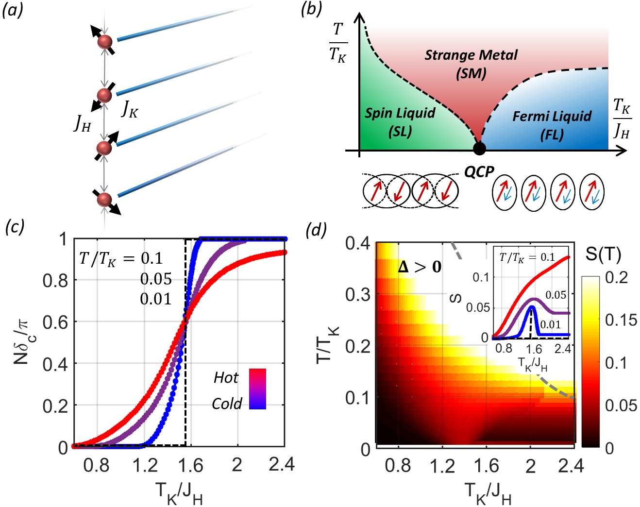
Figure 1: (color online) (a) Model 1D Kondo lattice, with local moments (red) with an AFM Heisenberg coupling $J_{H}$, individually screened by separate conduction electron baths (blue wires). (b) Schematic phase diagram showing the transition between heavy-Fermi liquid (FL) and spin-liquid (SL) phases at a QCP which evolves to a fan of strange metal (SM) at finite temperature. (c) Conduction electron phase shift $\delta_{c}$ as a function of $T_{K}/J_{H}$, which extrapolates to a step-like jump from $0$ to $\pi/N$ as $T\rightarrow 0$. (d) Color map of entropy $S(T)$, showing the collapse of energy scales at the QCP: the dashed line separates localized ($\Delta=0$ to the right) and delocalized ($\Delta>0$ to the left) spinon regimes. Inset: temperature cuts showing the accumulation of entropy at the QCP.

Watanabe and Miyake have argued that the development of soft charge fluctuations near a heavy fermion QCP is likely a result of a quantum-critical end-point, in which a first-order valence changing transition line is suppressed to low temperatures Watanabe and Miyake (2013); Miyake and Watanabe (2014); Watanabe and Miyake (2014, 2015); Scheerer et al. (2018). Here we present an alternative view, arguing that the coincidence of soft charge fluctuations and Kondo breakdown is a natural consequence of the Fermi surface collapse.

In the eighties, Anderson introduced the concept of a nominal valence to distinguish the valence of a rare earth ion infered from the apparent delocalization of f-electrons Anderson (1983); Aeppli and Fisk (1992), from the core-level valence, infered from spectroscopy. From this perspective, a shift in nominal valence is associated with formation of a large Fermi surface, even in a strict Kondo lattice where the core-level valence is fixed. Interpreted literally, this implies a kind of many-body ionization in the Kondo lattice, in which a fractionalization of local moments into charged heavy electrons, leaves behind a compensating positive background of Kondo singlets Lebanon and Coleman (2008). Taken to its logical extreme, such an interpretation would then imply that at KBD quantum critical point, degenerate fluctuations in the nominal valence will give rise to an observable soft charge mode.

While Kondo Breakdown has been extensively modelled at an impurity-level Pixley et al. (2012); Chowdhury and Ingersent (2015) and simulated using dynamical mean-field theory Si et al. (2001); De Leo et al. (2008); Martin et al. (2010), a possible link with charge fluctuations has not sofar been explored in the lattice. To examine this idea, we introduce a simple field-theoretic framework for Kondo breakdown, emplying a Schwinger boson representation of spins that permits us to treat Kondo screening and antiferromagnetism Parcollet and Georges (1997); Arovas and Auerbach (1988). Early application of this method demonstrated its efficacy for describing a ferromagnetic quantum critical point Komijani and Coleman (2018) in a Kondo lattice. Here we consider a Kondo screened one dimensional (1D) AFM [Fig. 1a], examining the quantum phase transition transition between a spin-liquid and a Fermi liquid [Fig. 1(b)]. The conduction electron phase shift (related to the Fermi surface size) jumps at $T=0$ [Fig. 1(c)], indicating that QCP is a KBD transition. Additionally, we find that the KBD features a zero point entropy [Fig. 1(d)]. In our calculations we observe that the KBD is linked to the emergence of a gapless charge degree of freedom at the QCP which occurs in natural coincidence with a divergent charge and staggered spin susceptibility.

Model - The simplified 1D Kondo lattice is a chain of antiferromagnetically coupled spins each individually screened by a conduction electron bath:

$$H=\sum_{j}\Big{[}H_{C}(j)+J_{K}\vec{S}_{j}\cdot\vec{\sigma}_{j}+J_{H}\vec{S}_{j}\cdot\vec{S}_{j+1}\Big{]}.$$ (1)

Here $\vec{S}_{j}$ is the spin at the $j$-th site, coupled antiferromagnetically to its neigbor with strength $J_{H}$. $H_{C}(j)=\sum_{{\bf p}}\epsilon_{{\bf p}}c^{\dagger}_{{\bf p}\alpha}(j)c_{{\bf p}\alpha}(j)$ describes the conduction bath coupled to the $j$-th moment in the chain, where ${\bf p}$ is the momentum of the conduction electron. $\vec{\sigma}_{j}=\psi^{\dagger}_{j\alpha}\vec{\sigma}_{\alpha\beta}\psi_{j\beta}$ is the spin density at site $j$, where $\psi^{\dagger}_{j\alpha}=\sum_{{\bf p}}c^{\dagger}_{{\bf p}\alpha}(j)$ creates an electron on the chain at site $j$.

Global phase diagram - Numerical and experimental studies of heavy-fermion systems are often interpreted Si et al. (2001); Coleman et al. (2001b); Coleman and Nevidomskyy (2010) within a global phase diagram of the Kondo lattice, with two axes: a Doniach parameter $x=T_{K}/J_{H}$ Doniach (1977), where $T_{K}$ is the Kondo temperature, and a frustration parameter $y$ representing the magnitude of quantum fluctuations, controlled by geometrical or dimensional frustration. The 1D limit provides a way to explore the two extremes of $y$: on the one hand, the uniform magnetization of a 1D FM commutes with the Hamiltonian and has no quantum fluctuations, corresponding to $y=0$ Komijani and Coleman (2018), whereas a 1D AFM never develops long range order, loosely corresponding to $y=\infty$. When the magnetic coupling is Ising-like, both models can be mapped to the dissipative transverse-field Ising model. But a Heisenberg magnetic coupling has been proven to be difficult to treat with these methods Lobos et al. (2012); Lobos and Cazalilla (2013) and a single formalism that can access various phases and critical points is highly desirable.

The method - We use a large-$N$ approach, obtained by enlarging the spin rotation group from SU(2) to SP($N$), representing the spin $S$ local moments using Schwinger bosons (“spinons”), according to $S_{\alpha\beta}=b^{\dagger}_{\alpha}b^{\vphantom{\dagger}}_{\beta}-\tilde{\alpha}\tilde{\beta}b^{\dagger}_{-\beta}b^{\vphantom{\dagger}}_{-\alpha}$Read and Sachdev (1991); Flint and Coleman (2009), where $\alpha\in[\pm 1,\dots\pm N/2]$, $\tilde{\alpha}={\rm sign}{(}\alpha)$ and $n_{b}(j)=2S$ is the number of bosons per site. Each moment is coupled to a $K$-channel conduction sea, with Hamiltonian

$$H=\sum_{j}\Big{[}H_{AFM}(j)+H_{K}(j)+H_{C}(j)+H_{\lambda}(j)\Big{]},$$ (2)

where

$$H_{AFM}(j) = -(J_{H}/N)(\tilde{\alpha}b^{\dagger}_{j\alpha}b^{\dagger}_{j+1,-\alpha})(\tilde{\beta}b^{\vphantom{\dagger}}_{j+1,-\beta}b^{\vphantom{\dagger}}_{j\beta}),$$

$$H_{K}(j) = -(J_{K}/N)\bigl{(}b^{\dagger}_{j\alpha}\psi^{\vphantom{\dagger}}_{ja\alpha}\bigr{)}(\psi^{\dagger}_{ja\beta}b^{\vphantom{\dagger}}_{j\beta}),$$

$$H_{\lambda}(j) = \lambda_{j}[n_{b}(j)-2S].$$ (3)

Here we have adopted a summation convention for the repeated greek $\alpha\in[\pm 1,\pm N/2]$ spin and roman $a\in[1,K]$ channel indices. The Lagrange multiplier $\lambda_{j}$ imposes the constraint $n_{b}(j)=2S$: we take $2S=K=2sN$ for perfect screening, where $s$ is kept fixed.

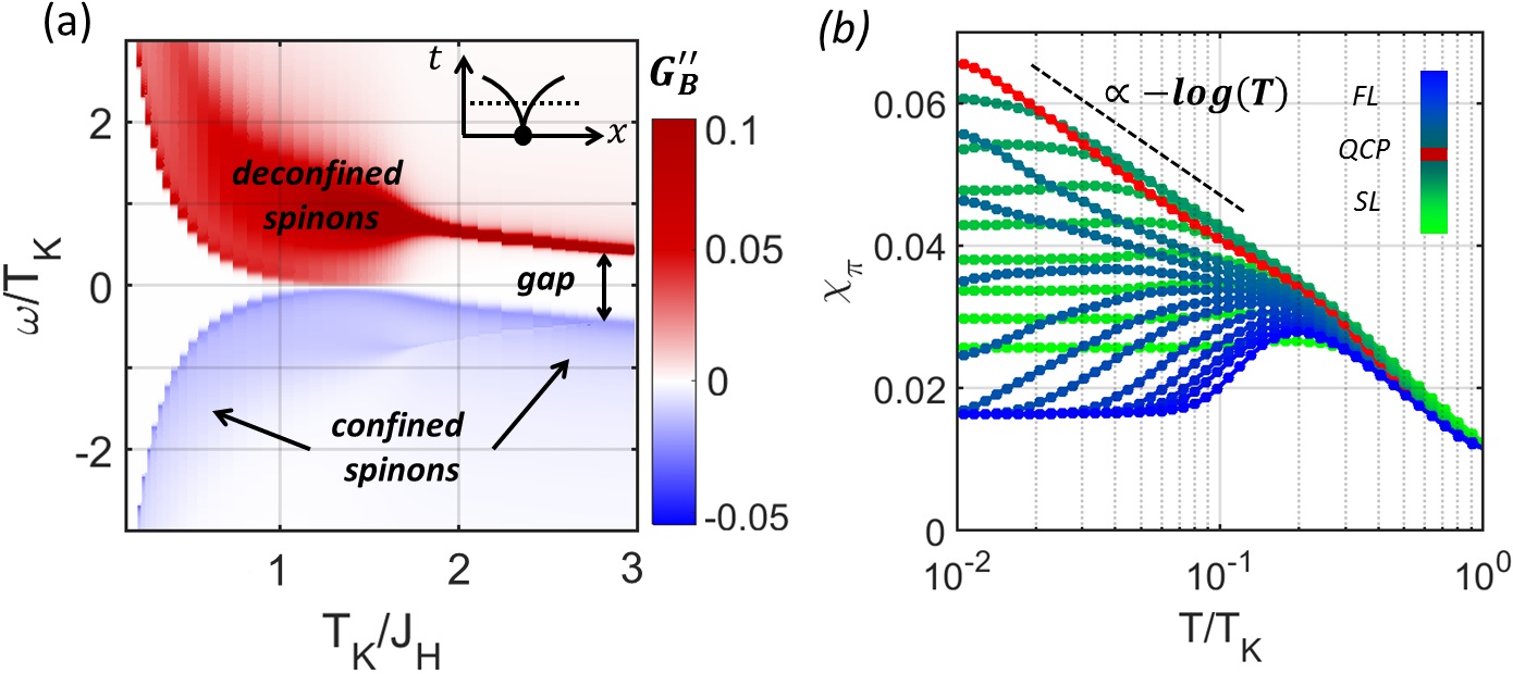
Figure 2: (color online) (a) Calculated spectral function of spinons $G_{B}^{\prime\prime}(\omega-i\eta)$ at $T/T_{K}=0.03$ shows confined spinons protected by a gap in the FL and SL, and deconfined with with a soft excitation gap in the SM regime. (b) Staggered spin susceptibilities vs. $T/T_{K}$ for various various values of $T_{K}/J_{H}$ from SL (in green) and FL (in blue) passing QCP (in red). A $\log$-divergence at the QCP is visible.

We carry out the Hubbard-Stratonovich transformations:

$$H_{K}(j) \to \bigl{[}(b^{\dagger}_{j\alpha}\psi^{\vphantom{\dagger}}_{ja\alpha})\chi_{ja}+{\rm h.c}\bigr{]}+\frac{N\bar{\chi}_{ja}\chi^{\vphantom{\dagger}}_{ja}}{J_{K}}$$ (4)

$$H_{AFM}(j) \to \bigl{[}\bar{\Delta}_{j}(\tilde{\alpha}b^{\dagger}_{j+1,-\alpha}b^{\dagger}_{j,\alpha})+{\rm h.c}\bigr{]}+\frac{N|\Delta_{j}|^{2}}{J_{H}},$$

where $\chi_{ja}$ is a Grassmanian “holon” field that mediates the Kondo effect at site $j$ in channel $a$, while $\Delta_{j}$ describes the development of singlets between site $j$ and $j+1$. See Komijani and Coleman (2018) For a discussion of spurious 1st order transition and their remedy.

A mean-field resonating valence-bond (RVB) description of the 1D magnetism is obtained from a uniform mean-field theory where $\Delta_{j}=i\Delta_{B}/2$, and $\lambda_{j}=\lambda$, giving rise to a bare spinon dispersion $\epsilon_{B}(p)=[{\lambda^{2}-\Delta_{p}^{2}}]^{\frac{1}{2}}$, with $\Delta_{p}=\Delta_{B}\sin p$. Both $b$ and $\chi$ fields have non-trivial dynamics Parcollet and Georges (1997); Parcollet et al. (1998); Coleman et al. (2005b); Rech et al. (2006); Komijani and Coleman (2018), with self-energies

$$\Sigma_{\chi}(\tau)=g_{0}(-\tau)G_{B}(\tau),\qquad\Sigma_{B}(\tau)=-\gamma g_{0}(\tau)G_{\chi}(\tau).$$ (5)

Here, $\gamma=K/N=2s$ and $G_{\chi}(\tau)$, $G_{B}(\tau)$ and $g(\tau)$ are the local propagators of the holons, spinons and conduction electrons, respectively. The conduction electron self-energy is of order ${\cal O}(1/N)$ and is neglected in the large-$N$ limit, so that $g_{0}(\tau)$ is the bare local conduction electron propagator. The holon Green’s function $G_{\chi}(z)=[{-J{{}_{K}}^{-1}-\Sigma_{\chi}(z)}]^{-1}$, is purely local, whereas the spinons are delocalized by the RVB pairing with propagator $\mathbb{G}_{B}(p,z)=[z\tau^{z}-\lambda\mathbb{1}-\Delta_{p}\tau^{{x}}-\mathbb{\Sigma}_{B}(z)]^{-1}$. The self-energy $\mathbb{\Sigma}_{B}(z)$ is diagonal in Nambu space, and the momentum sum in $\mathbb{G}_{B}^{\rm loc}(z)=\sum_{p}\mathbb{G}_{B}(p,z)$ can be done analytically SM .

Stationarity of the free energy with respect to $\lambda$ enforces the mean-field constraint $\langle n_{b}(j)\rangle=K$, and with respect to $\Delta_{B}$ determines the relation $\Delta_{B}(J_{H})$ SM . We solve these self-consistent equations numerically on the real-frequency axis using linear and logarithmic grids.

The two limits - In absence of Kondo screening (when $T_{K}/J_{H}$ is small) the constraint is satisfied with $\lambda>\Delta_{B}$. This Schwinger boson model describes a bipartite spin chain, in which each sublattice is in the symmetric spin-$S$ representation of SP($N$) Read and Sachdev (1991); Flint and Coleman (2009): Each spin can form singlets with its neighbors in an RVB state for any value $S$. This, together with the Gutzwiller projection treated by a soft constraint leads to a U(1) gapped spin liquid Arovas and Auerbach (1988), closely analogous to the integer-spin Haldane chain Haldane (1983). A lattice with closed boundary condition has a unique ground state and corresponds to a symmetry protected topological phase Pollmann et al. (2010).

The large $T_{K}/J_{H}$ limit corresponds to a local Fermi liquid Rech et al. (2006); Komijani and Coleman (2018) at each site of the chain, in which the electrons and spinons form bound, localized singlets, protected by a spectral gap of the size $T_{K}$; the remaining electrons are scattered with a phase shift $\delta_{c}=\pi/N$. Fig. (1b) summarizes the phase diagram as $T_{K}/J_{H}$ is varied between the above two limits, which we discuss in the following.

Ward identity, Entropy, Phase Shifts - At large $N$, the many body equations can be derived from a Luttinger Ward functional, leading to an exact relation between the conduction electron and holon phase shifts $\delta_{c}=\delta_{\chi}/N$ and a closed form formula for the entropy Coleman et al. (2005b); Rech et al. (2006). Fig. 1(c) shows the conduction electron phase shift $N\delta_{c}/\pi$ as a function of $T_{K}/J_{H}$. In the Fermi liquid, $\delta_{\chi}=N\delta_{c}$ is equal to $\pi$, equivalent to a large Fermi surface, but it is zero in the spin liquid regime. Extrapolating the calculations to $T\to 0$, the phase shift appears to jump at the QCP separating the spin-liquid (decoupled electrons) and the Fermi-liquid. From the perspective of conduction electrons, both SL and FL phases are Fermi liquids and the transition in $\delta_{\chi}$ is a measure of change in the Fermi surface, a manifestation of Kondo breakdown (KBD).

Entropy - Fig. 1(d) shows the colormap of the entropy $S(T)$ across the phase diagram. The gray dashed line indicates a second order phase transition for the internal variable $\Delta_{B}$ that separates a local Fermi liquid ($\Delta_{B}=0$) from a de-localized regime ($\Delta_{B}>0$). The collapse of the energy scale from both sides are visible. Unlike the 1D ferromagnetic QCP Komijani and Coleman (2018), the antiferromagnetic QCP develops a residual entropy $S_{E}/N\approx 1/20$ at a spin of $s=0.1$ per moment (inset of Fig. 1d),

Magnetic excitations - Fig. (2a) shows the spinon spectrum $G^{\prime\prime}_{B}(\omega-i\delta)$ vs. $T_{K}/J_{H}$ at $T/T_{K}=0.03$. Approaching the transition from the Fermi liquid side (right), the spinon spectrum shifts to positive frequencies and, maintaining overall gap size, brings the gap edge close to the chemical potential and only then, the hard gap closes at the QCP. Passing through the critical point, the gap re-opens due to development of short-range RVBs in the spin liquid regime. Fig. 2(b) shows the temperature dependence of the staggered spin susceptibility $\chi_{\pi}$, which acquires a logarithmic temperature dependence $\chi_{\pi}\sim-\log T$ at the QCP. The Fermi liquid (blue) exhibits a crossover from Curie law $1/T$ to a Pauli form $1/T_{K}$, with a characteristic peak at $T/T_{K}\sim 0.1$. As $T_{K}/J_{H}$ is reduced the peak position is unchanged (unlike the 1D FM case Komijani and Coleman (2018)) whereas the low temperature susceptibility develops a logarithmic divergence. Similar divergence is observed in local spin susceptibility but the uniform susceptibility is merely suppressed by the magnetism SM .

The holon spectrum - $G^{\prime\prime}_{\chi}(\omega-i\eta)$ shows a striking behavior at the QCP (Fig. 3a). Most of the spectral weight is contained in a sharp holon mode which crosses the chemical potential as $T_{K}/J_{H}$ is tuned from Fermi liquid (right) to spin-liquid (left). In the critical regime at a finite temperature, the holon mode is pinned to the Fermi energy over a finite range of Doniach parameter, which shrinks to a point as $T\to 0$, forming a strange metal (SM) regime at finite temperature with deconfined critical holon and spinon modes.

Figure 3: (a) Calculated spectrum of holons $G_{\chi}^{\prime\prime}(\omega-i\eta)$ showing that the holon mode crosses the chemical potential at the QCP. (b) $\omega/T$ scaling of the holon Green’s function $G^{\prime\prime}_{\chi}(\omega-i\eta)$ at the QCP. The inset shows the holon mode before scaling. (c) The ${\cal O}(1)$ charge vertex of holons coupling them to potential fluctuations. (d) The charge susceptibility computed via this vertex corrections (inset) shows a $T^{-1}$ divergence at the QCP point (red) and its suppression in SL/FL sides.

$\omega/T$ scaling - At the QCP, the holon mode lies at zero energy. Fig. 3(b) shows that the holon spectra at different temperatures collapse onto a single scaling curve $G^{\prime\prime}_{\chi}(\omega,T)=T^{-\alpha}f(\omega/T)$. For $s=0.1$ we find $\alpha=0.6$ consistent with a scaling analysis SM . The universality class of the QCP appears to be that of an overscreened impurity modelParcollet and Georges (1997) , with an effective number of channels $K_{\rm eff}/N=(1/\alpha-1)\approx 0.67>2s$.

The holon modes have an emergent coupling to the electromagnetic field, mediated via the internal vertices of the lattice Kondo effect. In particular, the field theory implies an ${\cal O}(1)$ vertex correction that couples to the electric potential as shown in Fig. 3(c). At low energies the vertex can be approximated by $\Gamma_{\chi}=-\frac{d}{d\omega}\Sigma_{\chi}$. This quantity perfectly cancels the wavefunction renormalization of the holon propagator $G_{\chi}\approx Z_{\chi}/\omega$, where $Z_{\chi}=-[\partial_{\omega}\Sigma_{\chi}]^{-1}$, so that the holon couples to the electric potential with a net charge $\Gamma_{\chi}Z_{\chi}=+1$. Fig. (3)(d) shows the charge susceptibility calculated using this vertex corrections. At the QCP, the temperature dependence of the holon charge susceptibilty acquires a Curie-like temperature dependence $\chi_{\rho}\sim 1/T$.

Discussion - We have studied a simplified Kondo lattice model in the large-$N$ limit, enabling us to extract the KBD physics directly on a lattice. It is illuminating to note that both specific heat and spin susceptibility SM disagree with the predictions of Hertz-Millis theories of the KBD based on using hybridization as an order parameter Paul et al. (2007); Pépin (2007).

One of the striking features of our description of the KBD quantum critical point is the presence of an emergent, spinless critical charge mode with a Curie-like charge susceptibility. Our model calculations can be extended in various ways, by going to higher dimensions, by generalizing to the mixed valence regime, and with considerable increase in computation, to a model in which a single bath is shared between all moments. In the general Kondo lattice, the charge conservation Ward identity links the change in the volume of the conduction electron Fermi surface $\Delta v_{FS}$ to the charge density of the Kondo singlets, described by the holon phase shift Coleman et al. (2005b)

$$N\frac{\Delta v_{FS}}{(2\pi)^{3}}=\overbrace{\sum_{{\bf p}}\frac{1}{\pi}{\rm Im}\ln\biggl{[}-G_{\chi}^{-1}({\bf p},z)\biggr{]}_{z=0+i\delta}}^{\delta_{\chi}/\pi}$$ (6)

Quite generally, the holon phase shift is zero or $\pi$ in the localized magnetic, or Fermi liquid phases respectively, but must jump between these two limits at the quantum critical point establishing critical holons. This and the O(1) charge vertex leads to critical charge fluctuations, independent of the details of the model. This strongly suggests that the gapless holon mode seen in our model calculation will persist at a more general Kondo breakdown quantum critical fixed point. Whether the Ward identity remains valid in models with reduced symmetry, is something we leave for future.

This raises the fascinating question how the predicted critical charge modes at KBD might be observed experimentally. One mode of observation, is via the coupling to nuclear Mossbauer lines Komijani and Coleman (2016). A recent observation of the splitting of the Mossbaüer line-shape  Kobayashi et al. (2018), characteristic of slow valence fluctuations, may be a fingerprint of these slow charge fluctuation.

Another interesting question is whether the residual entropy of the QCP might survive beyond the independent bath approximation. A residual ground-state entropy is a signature of infinite-range entanglement, and has been seen in various quantum models, such as the two channel Kondo model Andrei and Destri (1984); Tsvelik and Wiegmann (1984); Ludwig and Affleck (1994) or the Sachdev-Ye-Kitaev model Sachdev and Ye (1992); Georges et al. (2001); Maldacena and Stanford (2016). In the single-channel Kondo problem, the Kondo screening length Affleck (2010) $\xi_{K}\sim v_{F}/T^{\rm eff}_{K}$ plays the role of an entanglement length-scale, beyond which the singlet ground-state is disentangled from the conduction sea. If the collapse of the Kondo temperature $T_{K}^{\rm eff}\to 0$ at the QCP of a Kondo lattice involves a divergence of the entanglement length $\xi_{K}\to\infty$, the corresponding quantum critical point would be expected to exhibit an extensive entanglement entropy. Such naked quantum criticality is likely to be censored by competing ordered phases that consume the entanglement entropy of the critical regime, concealing QCP beneath a dome of competing phase, such as superconductivity.

Lastly, a peculiar feature of strange metals in heavy-fermions is that the resistivity tends to be linear in $T$ over a wide range of tempreature. At present, such behavior can be derived only from quenched disordered models Parcollet and Georges (1999). One of the fascinating implications of a Curie-law charge susceptibility $\chi_{\rho}\sim 1/T$ seen in our calculations, is that if combined with a temperature-independent diffusion of incoherent holon motion, it would give rise to a Curie conductivity (linear resistivity $\rho\propto 1/\sigma\sim T$) via the Einstein relation $\sigma=D\chi_{c}\sim 1/T$, where $D$ is the holon diffusion constant. This raises the interesting possibility that linear resistivities are driven by an emergent critical charge mode.

This work was supported by NSF grant DMR-1830707 (Piers Coleman), and by a Rutgers University Materials Theory postdoctoral fellowhsip (Yashar Komijani). We would like to thank S. Nakatsuji, H. Kobayashi, A. Vishwanath, J. Pixley, C. Chung and A. Georges for stimulating discussions, M. Oshikawa for helpful correspondence and A. M. Lobos, M. A. Cazalilla and P. Chudzinski for discussing that clarified the relation to Lobos et al. (2012); Lobos and Cazalilla (2013).

I Supplementary Material

This supplementary section contains additional details, proofs and calculations that are not included in the paper. For completeness, in section A, we include a bosonization mapping between the Ising limit of our model and the dissipative transverse field Ising model. In section B, we review the Arovas-Auerbach solution to the 1D antiferromagnet using the Schwinger boson representation of the spin. In C we provide the details of the dynamical large-$N$ equations, as well as formulas used to evaluate various thermodynamical properties. In section D we present a perturbative analysis of the large-$N$ equations showing that the phase shift jumps between $0$ and $\pi$. In section E we establish that at the QCP the renormalized energies of spinon and holon go to zero, and show that the critical exponent we found numerically is consistent with the scaling limit of large-$N$ equations. In section F we provide additional data on the holon phase shift and charge susceptibility to support the statements of the paper.

I.1 A. Mapping to the dissipative Transverse-field Ising model

In this section we use the bosonization technique to show that in the limit of purely Ising coupling between the magnetic moments (both ferromagnetic and antiferromagentic), our model can be mapped to a dissipative transverse-field Ising model. Such a mapping first appeared in Lobos et al. (2012). This is a property of the independent screening approximation and does not depend on the dimensionality of the spin lattice. The Hamiltonian is

$$H=-J_{H}\sum_{n}\vec{S}_{n}\cdot\vec{S}_{n+1}+J_{K}\sum_{n}\vec{S}_{n}.\vec{s}_{n}+H_{C}.$$ (7)

Let us write the Hamiltonian in the general anisotropic form

$$H = -\sum_{n}\Big{[}J_{H}^{z}S_{n}^{z}S_{n+1}^{z}+{J_{H}^{\perp}}\Big{(}S_{n}^{x}S_{n+1}^{x}+S_{n}^{y}S_{n+1}^{y}\Big{)}\Big{]}$$ (9)

$$+\sum_{n}\Big{[}J_{K}^{z}S_{n}^{z}s^{z}_{n}+\frac{J_{K}^{\perp}}{2}\Big{(}S^{+}_{n}s_{n}^{-}+h.c.\Big{)}\Big{]}+H_{C}.\qquad$$

In the continuum limit, $H_{C}$ is

$$H_{C} = -iv_{F}\sum_{n\sigma}\int_{0}^{\infty}{dx[\psi^{\dagger}_{Rn\sigma}\partial_{x}\psi^{\vphantom{\dagger}}_{Rn\sigma}-\psi^{\dagger}_{Ln\sigma}\partial_{x}\psi^{\vphantom{\dagger}}_{Ln\sigma}]}$$

$$\to -iv_{F}\sum_{n\sigma}\int_{-\infty}^{+\infty}{dx\psi^{\dagger}_{Rn\sigma}\partial_{x}\psi^{\vphantom{\dagger}}_{Rn\sigma}}.$$

At $x=0$ we have the boundary condition $\psi_{R}(x=0)=\psi_{L}(x=0)$. We have unfolded the semi-infinite wire into a single set of right-movers which interact (via a Kondo interaction) with the impurities at the origin. Next, we bosonize:

$$\psi_{Rn\sigma}\sim\exp[{i\sqrt{2\pi}\varphi_{Rn\sigma}}],\qquad:\psi^{\dagger}_{R}\psi^{\vphantom{\dagger}}_{R}:=\frac{\partial_{x}\varphi_{R}}{\sqrt{2\pi}}.$$ (11)

We can introduce charge and spin bosons $\sqrt{2}\varphi_{c/s}=\varphi_{\uparrow}\pm\varphi_{\downarrow}$ and only spin-bosons appear in the Hamiltonian. The conduction-band spin is given by

$$2s^{z}_{n} = \psi^{\dagger}_{Rn\uparrow}\psi^{\vphantom{\dagger}}_{Rn\uparrow}-\psi^{\dagger}_{Rn\downarrow}\psi^{\vphantom{\dagger}}_{Rn\downarrow}\to\frac{\partial_{x}\varphi_{n,s}}{\sqrt{\pi}},$$ (12)

$$s^{+}_{n} = \psi^{\dagger}_{Rn\uparrow}\psi^{\vphantom{\dagger}}_{Rn\downarrow}\to\exp[i2\sqrt{\pi}\varphi_{n,s}(0)].$$ (13)

The bosonized Hamiltonian is then

$$H = -\sum_{n}\Big{[}J_{H}^{z}S_{n}^{z}S_{n+1}^{z}+\frac{J_{H}^{\perp}}{2}\Big{(}S_{n}^{+}S_{n+1}^{-}+h.c.\Big{)}\Big{]}+H_{C}$$

$$+ \sum_{n}\Big{[}\frac{J_{K}^{z}}{2\sqrt{\pi}}S_{n}^{z}\partial_{x}\varphi_{n,s}(0)+\frac{J_{K}^{\perp}}{2}\Big{(}S^{+}_{n}e^{i2\sqrt{\pi}\varphi_{n,s}}+h.c.\Big{)}\Big{]}.$$

We also note that

$$H_{C}=\frac{v_{F}}{2}\sum_{n}\int_{-\infty}^{+\infty}{[(\partial_{x}\varphi_{c})^{2}+(\partial_{x}\varphi_{s})^{2}]}.$$ (14)

Next we apply the Emery-Kievelson transformation to simplify the Kondo interaction

$$U_{\alpha}=\prod_{n}\exp[i\alpha S^{z}_{n}\varphi_{n,s}(0)].$$ (15)

Using the identities

$$U^{\dagger}\frac{\partial_{x}\varphi_{s}}{\sqrt{2\pi}}U = \frac{\partial_{x}\varphi_{s}}{2\sqrt{\pi}}-\frac{\alpha}{\sqrt{2\pi}}S^{z}\delta(x),$$ (16)

$$U^{\dagger}S_{n}^{+}e^{i2\sqrt{\pi}\varphi_{s}}U = S_{n}^{+}e^{i(2\sqrt{\pi}-\alpha)\varphi_{s}},$$ (17)

and choosing $\alpha=2\sqrt{\pi}$, the transverse Kondo coupling is eliminated, and we then have

$$U^{\dagger}HU = -\sum_{n}J_{H}^{z}S_{n}^{z}S_{n+1}^{z}+\sum_{n}\Big{[}J_{K}^{\perp}S_{n}^{x}$$

$$+(\frac{J^{z}_{K}}{2\sqrt{\pi}}-\frac{\alpha}{\sqrt{2\pi}\rho})S^{z}_{n}\partial_{x}\varphi_{n,s}\Big{]}+H_{C}+H_{\perp}[J_{H}^{\perp}].$$

We have only explicitly written the Ising part of Ferromagnetic coupling and have moved the remaining terms into $H_{\perp}$. If we choose $\rho J^{z}_{K}=\sqrt{2}$, the Ising part of Kondo interaction then drops out and the transverse Kondo interaction appears as a Zeeman field acting on the “dressed spin”. This is called the “Decoupling point” and constitutes an additional solvable point of the single-impurity Kondo model, similar to the “Toulouse point”. The Kondo temperature of this highly anisotropic Kondo system is $T_{K}=J_{H}$. Therefore, assuming $J_{H}^{\perp}=0$, we have

$$J_{H}^{\perp}=0,\qquad\to\quad H=-\sum_{n}J_{H}^{z}S_{n}^{z}S_{n+1}^{z}+\sum_{n}T_{K}S_{n}^{x},$$ (19)

which is the transverse-field Ising model. This model can be re-written using a Jordan-Wigner transformation in terms of two Majorana fermions with a gap that changes sign at the QCP separating the disordered and ordered phases. Moving away from the Decoupling point introduces an additional $\delta S^{z}\partial_{x}\varphi$ term into the Hamiltonian which implies that the spins are now dissipatively coupled to a gapless bosonic bath.

If $J_{H}^{\perp}\neq 0$, we have

$$U^{\dagger}H_{\perp}U = -\frac{J_{H}^{\perp}}{2}\sum_{n}\Big{(}S_{n}^{+}S_{n+1}^{-}e^{i\alpha[\varphi_{sn}-\varphi_{s,n+1}]}+h.c.\Big{)}.$$

At the strong Kondo coupling fixed point, Ref. Lobos et al. (2012) projects out the magnetic moments, mapping the problem to a dissipative Josephson Junction array which is further mapped to a Hertz-Millis theory. This corresponds to a spin-density instability of heavy-fermions [private communication], (which is absent in our large-$N$ approach, presumably due to the fact that conduction electron self-energy is $O(1/N)$), rather than the deconfined criticality discussed in this work.

I.2 B. Review of the Arovas-Auerbach approach

Here, we review the Arovas-Auerbach Arovas and Auerbach (1988) approach to 1D antiferromagents. In the momentum space we have

$$H=\sum_{\alpha}\lambda b^{\dagger}_{k\alpha}b^{\vphantom{\dagger}}_{k\alpha}+\sum_{\alpha>0}\Delta_{k}(b^{\dagger}_{k\alpha}b^{\dagger}_{-k,-\alpha}+h.c.)-2S\lambda.$$ (20)

Here, the Lagrange multiplier enforces the constraint $n_{B}=2S=2sN$ necessary for a Schwinger boson representation of the spin. Using a Bogoliubov-de Gennes (BdG) transformation, we have

$$\left(\begin{array}[]{cc}b_{k\alpha}\\ b^{\dagger}_{-k,-\alpha}\end{array}\right)=\left(\begin{array}[]{cc}\cosh\theta_{k}&\sinh\theta_{k}\\ \sinh\theta_{k}&\cosh\theta_{k}\end{array}\right)\left(\begin{array}[]{cc}\beta_{k\alpha}\\ \gamma^{\dagger}_{k\alpha}\end{array}\right)$$ (21)

We can diagonalize the Hamiltonian by tuning $\tanh 2\theta_{k}=-\Delta_{k}/\lambda$ with energy $E_{k}=\sqrt{\lambda^{2}-\Delta_{k}^{2}}$, so that

$$H=\sum_{k\alpha}[E_{k}(\beta^{\dagger}_{k\alpha}\beta_{k\alpha}+\gamma^{\dagger}_{k\alpha}\gamma^{\vphantom{\dagger}}_{k\alpha})+(E_{k}-\lambda)]-2S\lambda$$ (22)

Constraint - We can write

$$2s = \frac{1}{NL}\sum_{k\alpha}\left\langle b^{\dagger}_{k\alpha}b^{\vphantom{\dagger}}_{k\alpha}\right\rangle$$

$$= \frac{1}{L}\sum_{k}[\cosh^{2}\theta_{k}\left\langle\beta^{\dagger}\beta\right\rangle+\sinh^{2}\theta_{k}\left\langle\gamma\gamma^{\dagger}\right\rangle]$$

which at zero temperature becomes

$$4s=\frac{1}{L}\sum_{k}[\cosh 2\theta_{k}-1].$$ (24)

In 1D we have $\Delta_{k}=\Delta_{B}\sin k$. Since $\cosh 2\theta_{k}=\lambda/E_{k}$, using $\kappa=\Delta_{B}/\lambda<1$ we then find

$$4s+1=\int_{-\infty}^{+\infty}{\frac{dk}{2\pi}}\frac{1}{\sqrt{1-\kappa^{2}\sin^{2}k}}=\frac{2}{\pi}K(\kappa),$$ (25)

where $K(\kappa)$ is the complete elliptic integral of first kind. Parametrizing $\kappa=\cos(\vartheta)$, near $\kappa\sim 1$ we have

$$4s+1=\frac{2}{\pi}K(\cos\vartheta)\approx-\frac{2}{\pi}\log(\vartheta/2),$$ (26)

so that the gap in the spectrum is proportional to

$$E_{g}=2\Delta_{B}\tan(\vartheta)\approx\Delta_{B}e^{-\pi(1+4s)/2}.$$ (27)

I.3 C. Details of large-$N$ compuations

The self-energies of spinons and bosons are

$$\Sigma_{B}(\tau)=-2sg_{c}(\tau)G_{\chi}(\tau),\quad\Sigma_{\chi}(\tau)=g_{c}(-\tau)G_{\chi}(\tau).$$

When written in the frequency domain and analytically continued onto the real frequency axis, the self energies become

$$\Sigma_{B}(\omega+i\eta) = \gamma\int_{-\infty}^{+\infty}{\frac{d\omega^{\prime}}{\pi}}f(\omega^{\prime})\Big{\{}g_{c}^{\prime\prime}(\omega^{\prime})G^{R}_{\chi}(\omega-\omega^{\prime})$$ (28)

$$\hskip 56.9055pt-g^{R}_{c}(\omega+\omega^{\prime})G_{\chi}^{\prime\prime}(-\omega^{\prime})\Big{\}},\qquad$$

$$\Sigma_{\chi}(\omega+i\eta) = \int_{-\infty}^{+\infty}{\frac{d\omega^{\prime}}{\pi}}\Big{[}-G_{B}^{R}(\omega+\omega^{\prime})f(\omega^{\prime})g_{c}^{\prime\prime}(\omega^{\prime})\qquad$$ (29)

$$\qquad+G_{B}^{\prime\prime}(\omega^{\prime})n_{B}(\omega^{\prime})g_{c}(\omega^{\prime}-\omega-i\eta)\Big{]}.$$

In this expression all the functions are retarded ($G^{R}(\omega)\equiv G(\omega+i\delta)=G^{\prime}(\omega)+iG^{\prime\prime}(\omega)$) and

$$g_{c}(z)=\sum_{k}\frac{1}{z-\epsilon_{k}}.$$ (30)

The propagator for the holon is local:

$$G_{\chi}^{-1}(z)=-\frac{1}{J}-\Sigma_{\chi}(z).$$ (31)

By contrast, the p-wave pairing in the spinon Hamiltonian gives rise to an anomalous pairing component in the spinon Green’s functions, causing the spinons to delocalize. The $G_{B}(z)$ appearing in the self-energies is the local Green’s function in which the anomalous components cancel out due to momentum-summation,

$$G_{B}(z)\equiv\Big{[}{\mathbb{G}}_{B}^{\rm loc}(z)\Big{]}_{pp}.$$ (32)

To see this explicitly, the spinon Greens function is given by

$${\mathbb{G}}_{loc}(z)=\sum_{q}\frac{1}{z\tau^{z}-{\mathbb{H}}_{B}-{\mathbb{\Sigma}}_{B}}.$$ (33)

This momentum-sum can be performed analytically which significantly accelerates the computation. First we write

$${\mathbb{G}}_{B}(q,z)=\frac{1}{z\tau^{z}-{\mathbb{H}}_{B}-{\mathbb{\Sigma}}_{B}}=\frac{1}{\Omega_{B}\tau^{z}-\Lambda_{B}\mathbb{1}+\Delta_{q}\tau^{x}},$$

where we have used the fact that the self-energy given in Eq. (28) is diagonal in the Nambu space, involving two components, $\bar{\Sigma}_{B}$ and $\delta\Sigma_{B}$,

$${\mathbb{\Sigma}}_{B}=\bar{\Sigma}_{B}\mathbb{1}+\tau^{z}\delta\Sigma_{B},$$ (34)

and we have defined

$$\qquad\Omega_{B}\equiv z-\delta\Sigma_{B},\qquad\Lambda_{B}\equiv\lambda+\bar{\Sigma}_{B}.$$ (35)

Using this short-hand notation, we have

$${\mathbb{G}}(q,z)=\frac{\Omega_{B}\tau^{z}-\Delta_{q}\tau^{x}+\Lambda_{B}\mathbb{1}}{\Omega_{B}^{2}+\Delta_{q}^{2}-\Lambda_{B}^{2}}=\frac{\mathbb{b}+\mathbb{c}\sin q}{\cos 2q+a},$$ (36)

where we have defined

$$a = \frac{2}{\Delta_{B}^{2}}[\Lambda_{B}^{2}-\Omega_{B}^{2}]-1,$$ (37)

$$\mathbb{b} = -\frac{2}{\Delta_{B}^{2}}[\Omega_{B}\tau^{z}+\Lambda_{B}\mathbb{1}],\hskip 5.69046pt\mathbb{c}=-\frac{2\tau^{x}}{\Delta_{B}}.\hskip 5.69046pt$$ (38)

The momentum-sum gives

$${\mathbb{G}}_{loc}(z) = \sum_{q}{\mathbb{G}}(q,z)=\int_{-\pi}^{\pi}\frac{dq}{2\pi}\frac{\mathbb{b}+\mathbb{c}\sin q}{\cos 2q+a}$$ (39)

$$= \int_{-\pi}^{\pi}\frac{\mathbb{b}}{\cos q+a}=\frac{\mathbb{b}}{a\sqrt{1-a^{-2}}},$$ (40)

which is diagonal in Nambu space with the particle-particle element proportional to $b_{pp}={\rm Tr}[b(1+\tau_{3})]/2=-2[\Omega_{B}+\Lambda_{B}]/\Delta_{B}^{2}$.

Saddle-point equations - Stationarity of the Free energy with respect to $\lambda$ and $\Delta$ then leads to the saddle-point equation

$$-\int_{-\infty}^{+\infty}{\frac{d\omega}{\pi}n_{B}(\omega){\rm Im}\left[G^{pp}_{B,loc}(\omega+i\eta)\right]}=2s,$$ (41)

$$\frac{1}{2J_{H}}=-\int{\frac{2d\omega}{\pi\Delta_{B}}}[n_{B}(\omega)+\frac{1}{2}]{\rm Im}\Big{\{}\sum_{p}\sin pG^{ph}_{B}(p,\omega+i\eta)\Big{\}},$$

which determine $\lambda$ and $J_{H}$ self-consistently. The momentum sum can be done analytically and we find

$$\frac{1}{J_{H}}=\int{\frac{4d\omega}{\pi\Delta_{B}}}[n_{B}(\omega)+\frac{1}{2}]{\rm Im}\Big{\{}\frac{1}{\Delta_{B}}\frac{1+a}{a\sqrt{1-a^{-2}}}\Big{\}}.$$ (42)

The calculations start at high temperature $T\gg T_{K}$ and the temperature is gradually reduced. Due to development of sharp features in the spectrum at low-temperatures and the importance of high-frequency components, more frequency points are required to achieve lower temperatures, a time/memory cost that eventually limits the lowest temperatures achieved.

Having computed the Green’s functions, we can use them to calculate various thermodynamical properties:

Susceptibility - The spin correlation function in SP($N$) is

$$\chi(n,\tau) \equiv \sum_{\alpha\beta}\left\langle-TS^{\alpha\beta}(n,\tau)S^{\beta\alpha}\right\rangle$$ (43)

$$= -{\rm Tr}\Big{[}\mathbb{G}_{B}(-n,-\tau)\tau^{z}\mathbb{G}_{B}(n,\tau)\tau^{z}\Big{]}.$$ (44)

The static susceptibility can be obtained by doing the imaginary-time integral of this correlation function which can be written in the form

$$\chi(q,0) = \int_{0}^{\beta}{d\tau}\sum_{\alpha\beta}\left\langle-TS^{\alpha\beta}(n,\tau)S^{\beta\alpha}\right\rangle$$ (45)

$$= \int{\frac{d\omega}{\pi}}n_{B}(\omega)\chi^{\prime\prime}_{B}(q,\omega),$$ (46)

where

$$\chi_{B}(q,\omega)\equiv\sum_{k}{\rm Tr}\Big{[}{\mathbb{G}}_{B}(k+q,\omega+i\eta)\tau^{z}{\mathbb{G}}_{B}(k,\omega+i\eta)\tau^{z}\Big{]}.$$ (47)

As in the previous case, the momentum-sum can be performed analytically. For uniform and staggered susceptibility this gives

$$\chi_{B}(0/\pi,\omega) = \frac{8}{\Delta^{4}}\frac{\Omega_{B}^{2}+\Lambda_{B}^{2}\mp(1+a_{B})\Delta_{B}^{2}/2}{a_{B}^{2}(1-a_{B}^{-2})^{3/2}}$$ (48)

$$\pm \frac{4}{\Delta_{B}^{2}}\frac{1}{a_{B}\sqrt{1-a_{B}^{-2}}}.$$ (49)

For the local susceptibility, we sum Eq. (47) over $q$ and find

$$\chi_{B}^{\rm loc}(\omega) = \sum_{k}{\rm Tr}\Big{[}\mathbb{G}_{B}^{\rm loc}(\omega+i\eta)\tau^{z}\mathbb{G}_{B}^{\rm loc}(\omega+i\eta)\tau^{z}\Big{]},$$ (50)

$$= [G_{B,loc}^{pp}]^{2}+[G_{B,loc}^{hh}]^{2}$$ (51)

to be inserted in Eq. (46). Fig. 4(a,b) show the uniform and local spin susceptibilities. While $\chi_{loc}$ diverges at the QCP, $\chi_{0}$ is only suppressed to zero by the antiferrmagnetism.

Entropy - The derivation of the entropy has been discussed in Rech et al. (2006) and Komijani and Coleman (2018). The free energy can be expressed as a stationary functional with respect to $G_{B}$, $G_{\chi}$ and $\lambda$ Komijani and Coleman (2018). Keeping those constant, we take derivative w.r.t $T$ to obtain the entropy. The result is Rech et al. (2006)

$$S(T) = -\int\frac{d\omega}{\pi}\partial_{T}n_{B}(\omega)\Big{\{}{\rm Im}\left[{\cal S}_{B}(\omega)\right]+\Sigma^{\prime\prime}_{B}(\omega)G^{\prime}_{B}(\omega)\Big{\}}$$ (52)

$$-k\int\frac{d\omega}{\pi}\partial_{T}f(\omega)\Big{\{}{\rm Im}\left[\log[-G_{\chi}^{-1}(\omega)]\right]$$

$$\hskip 85.35826pt+\Sigma^{\prime\prime}_{\chi}(\omega)G^{\prime}_{\chi}(\omega)$$

$$\hskip 85.35826pt-g^{\prime\prime}_{c}(\omega)\tilde{\Sigma}^{\prime}_{c}(\omega)\Big{\}}.$$

Here, all the greens functions are retarded $G(\omega)\equiv G(\omega+i\eta)$ and $g_{c}$ is the bare Green’s function of conduction band (30). And $\tilde{\Sigma}_{c}(\tau)=N\Sigma_{c}(\tau)$ where $\Sigma_{c}(\tau)=\frac{1}{N}G_{B}(\tau)G_{\chi}(-\tau)$ is the self-energy of the conduction electrons, which in the frequency domain is

$$\tilde{\Sigma}_{C}(\omega+i\eta) = \int{\frac{d\nu}{\pi}}\Big{[}n_{B}(\omega)G^{\prime\prime}_{B}(\nu+i\eta)G_{\chi}(\nu-\omega-i\eta)\qquad$$ (54)

$$\qquad-f(\nu)G^{\prime\prime}_{\chi}(\nu)G_{B}(\omega+\nu+i\eta)\Big{]}.$$

The function ${\cal S}_{B}(z)$ is part of the spinon contribution to the entropy that requires a momentum-summation:

$${\cal S}_{B}(z) = \frac{1}{2}\sum_{q}\log\Big{[}\det\{-G_{B}^{-1}(z,q)\}\Big{]}.$$ (55)

Again, this momentum sum can be done analytically to obtain

$${\cal S}_{B}(z) = \frac{1}{2}\sum_{q}\log[\Lambda_{B}^{2}-\Omega_{B}^{2}-\Delta_{B}^{2}\sin^{2}q]$$ (56)

$$= cte+\frac{1}{2}\sum_{q}\log[\cos 2q+a]$$ (57)

$$\to \frac{1}{2}\int{da}\sum_{a}\frac{1}{\cos q+a}$$ (58)

$$= \frac{1}{2}\log[a(1+\sqrt{1-a^{-2}})].$$ (59)

The specific heat is obtained from numerical differentiation of the $S(T)$. Fig. 5 shows the specific heat coefficient as a function of $T_{K}/J_{H}$ and $T/T_{K}$. The collapse of energy scale from both sides are visible. The suppression of the $C/T$ at the QCP implies a zero-point entropy due to entropy balance.

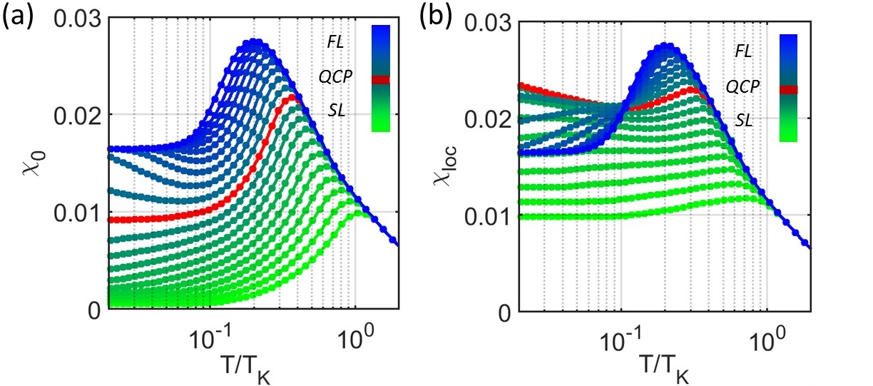
Figure 4: (a) The uniform $\chi_{0}$ and (b) the local $\chi_{loc}$ spin susceptibility vs. $T/T_{K}$ for various values of the tuning parameter $T_{K}/J_{H}$. While $\chi_{loc}$ diverges logarithmically at the QCP, the uniform susceptibility is only suppressed by the magnetism.

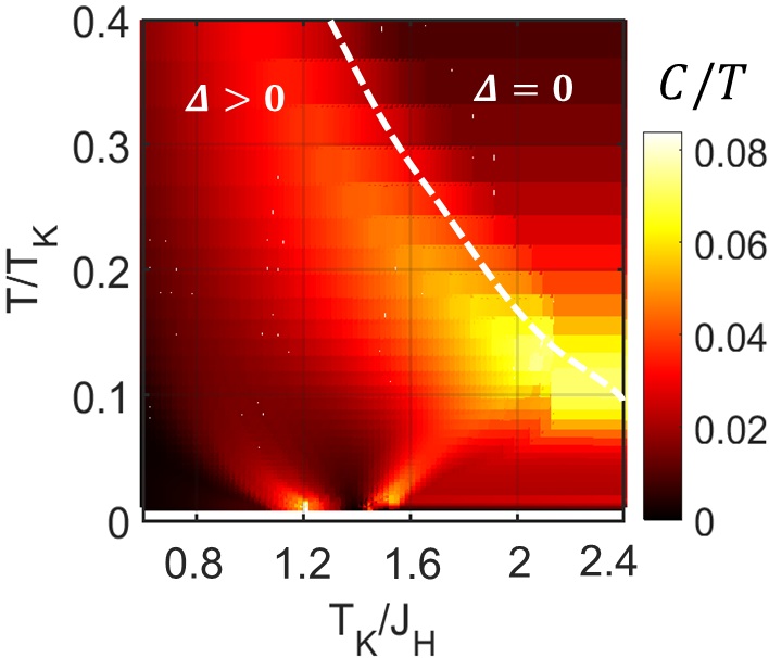
Figure 5: The specific heat coefficient $C/T=dS/dT$ vs. $T_{K}/J_{H}$ and $T/T_{J}$ shows the collapse of the energy scale from both sides as well as a suppression of the $C/T$ at the QCP, consistent with a zero-point entropy.

I.4 D. The leading order solution

Although, we have numerically obtained the solution to the self-consistent large-$N$ equations, it is interesting to study the results of a single-iteration of these equations.

In a simple antiferromagnet, the particle-particle component of the spinon Green’s function is

$$G^{pp}_{B}(q,z)=\frac{z+\lambda}{z^{2}-E_{q}^{2}}=\frac{u_{q}^{2}}{z-E_{q}}-\frac{v_{q}^{2}}{z+E_{q}},$$ (60)

where $E_{q}=\sqrt{\lambda^{2}-\Delta_{q}^{2}}$, $u=\cosh\theta_{q}$, $v=\sinh\theta_{q}$ and $\tanh 2\theta_{q}=-\Delta_{q}/\lambda$. Substituting this into (29), we obtain

$$\Sigma_{\chi}(z)=\sum_{k,q}\Big{\{} \frac{u^{2}_{q}[f(\epsilon_{k})+n_{B}(E_{q})]}{z-(E_{q}-\epsilon_{k})}$$ (61)

$$\hskip 42.67912pt+\frac{v_{q}([1-f(\epsilon_{k})+n_{B}(E_{q})]}{z-(\epsilon_{k}+E_{q})}\Big{\}}.\qquad$$

Using a flat density of states for $\epsilon_{k}$, at $T=0$ we find

$$\Sigma_{\chi}(z)=-\rho\sum_{q}\Big{\{} u^{2}_{q}\ln\left(\frac{D}{E_{q}-z}\right)-v^{2}_{q}\ln\left(\frac{D}{E_{q}+z}\right)\Big{\}}.\qquad$$ (62)

To obtain a rough estimate of this quantity, we can replace $E_{q}\sim\Delta$ by the typical energy of a spinon, so that

$$G_{\chi}^{-1}(z) = -\frac{1}{J}+\rho\left[u^{2}\ln\left(\frac{\Lambda}{\Delta-z}\right)-v^{2}\ln\left(\frac{\Lambda}{\Delta+z}\right)\right].$$ (63)

$$= \rho\left[u^{2}\ln\left(\frac{T_{K}}{\Delta-z}\right)-v^{2}\ln\left(\frac{T_{K}}{\Delta+z}\right)\right],$$ (64)

where we have used $u^{2}-v^{2}=1$, $T_{K}=\Lambda e^{-1/\rho J}$. The phase shift at zero frequency is given by

$$\delta_{\chi} = {\rm Im}\ln[G_{\chi}^{-1}(\omega+i\eta)]_{\omega=0}$$ (65)

$$= {\rm Im}\ln\left[\ln\left(\frac{\Delta+i\delta}{T_{K}}\right)\right]$$ (66)

$$= \pi\theta(T_{K}-\Delta).$$ (67)

While this is a crude approximation, it captures the key feature that the holon field $\chi$ first develops a bound-state when $T_{K}$ becomes of order $\Delta$.

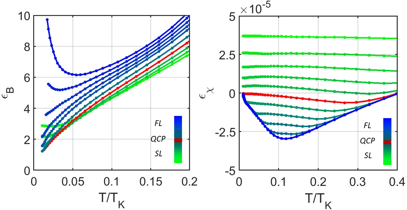
Figure 6: (a) A plot of $\varepsilon_{B}\equiv\lambda+\Sigma^{\prime}_{B}(0)-\Delta$ vs. $T$ for various values of Doniach parameter. (b) A plot of $\varepsilon_{\chi}\equiv 1/J+\Sigma^{\prime}_{\chi}(0)$ vs $T$ in various regimes.

I.5 E. Scaling conditions

Fig. 6 shows the renormalized energies of spinons $\varepsilon_{B}\equiv\lambda+\Sigma^{\prime}_{B}(0)-\Delta$ and holons $\varepsilon_{\chi}\equiv 1/J+\Sigma^{\prime}_{\chi}(0)$. We find that $\varepsilon_{B}\to 0$ and $\varepsilon_{\chi}\to 0$ in the $T\to 0$ limit at the QCP, whereas in SL, or FL regimes, $\varepsilon_{B}$ remains finite.

In the FL regime, $\varepsilon_{\chi}$ becomes negative at a finite temperautre, indicating electron-spinon bound state formation. At the QCP, $\varepsilon_{\chi}\to 0^{+}$ as $T\to 0$ meaning that $\delta\Sigma_{\chi}G_{\chi}=-1$, whereas in the SL regime, $\varepsilon_{\chi}$ remains finite.

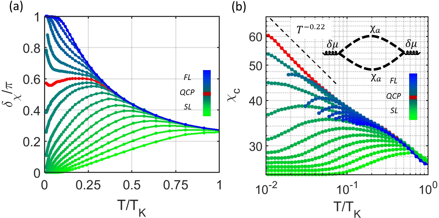
Figure 7: (a) The holon phase shift $\delta_{\chi}/\pi$ as a function of $T/T_{K}$, as $T_{K}/J_{H}$ is tuned from SL (green) to FL (blue) passing SM (red). (b) The holon-bubble vs. $T/T_{K}$ as the Doniach parameter is tuned from SL (green) to FL (blue) passing SM (red). The exponents at the SL-SM transition has a $T^{-0.2}$ divergence in agreement with the exponent extracted from $\omega/T$-scaling.

The collapse of the holon spectrum on the form $G^{\prime\prime}_{\chi}\sim T^{-\alpha}f(\omega/T)$, (where $\alpha=0.6$ at the specific value of $s=S/N=0.1$ studied in the numerical work presented here) implies that at zero temperature, $G_{\chi}(\omega)\sim\omega^{-\alpha}\Rightarrow G_{\chi}(\tau)\sim\tau^{\alpha-1}$. We showed that at the QCP $\varepsilon_{\chi}\to 0$. Therefore, the scaling limit of NCA equations can be used to find

$$G_{\chi}\sim\omega^{-\alpha}\sim\tau^{\alpha-1},\qquad \Sigma_{B}\sim\tau^{\alpha-2}\sim\omega^{1-\alpha}$$ (68)

$$\Sigma_{\chi}\sim\omega^{\alpha}\sim\tau^{-(1+\alpha)},\qquad G_{B}\sim\tau^{-\alpha}\sim\omega^{\alpha-1},$$ (69)

at the QCP, without invoking the relation between $G_{B}$ and $\Sigma_{B}$. The fact that $\varepsilon_{B}\to 0$ at the QCP and $\omega$-powers are cancelled in $\Sigma_{B}G_{B}$ shows that the QCP is a local one. This is in contrast to the FM case Komijani and Coleman (2018) where $G_{B}\sqrt{\Sigma_{B}}$ was involved.

The leading critical exponent of $G_{B}\sim\tau^{-\alpha}$ contributes a temperature-independent term to the local susceptibility $\chi_{loc}=\int_{0}^{\beta}{d\tau G_{B}(\tau)G_{B}(-\tau)}$ that depends on the UV cut-off. The log-behavior of $\chi_{\rm loc}$ shows that the sub-leading term in $G_{B}$ must contain a $\tau^{-0.5}$ term.

From $G_{\chi}\sim\tau^{\alpha-1}$ it follows that the holon bubble defined as $\chi_{c}=\int_{0}^{\beta}{d\tau G_{\chi}(\tau)G_{\chi}(-\tau)}\sim T^{1-2\alpha}$ diverges at low-temperatures, which is indeed confirmed numerically as we see in the next section.

I.6 F. Additional data on holons and spinons

Fig. 7(a) shows the holon phase shift $\delta_{\chi}/\pi$ as a function of $T/T_{K}$ for various values of the Doniach parameter $T_{K}/J_{H}$ tuned from FL to SL through the strange metal phase. Note that except at the SL-SM transition, all other phase shifts have a finite slope with temperature (at low-temperature) and approach the two fixed points logarithmically. Fig. 7(b) shows the holon bubble $\chi_{c}=\int_{0}^{\beta}{d\tau G_{\chi}(\tau)G_{\chi}(-\tau)}$ as $T_{K}/J_{H}$ is tuned between FL to SL through the QCP. The divergence at the QCP fits a $T^{-0.22}$ power-law in good agreement with the $T^{-0.2}$ power deduced from the $\omega/T$-scaling.

A derivation of full scaling form of Green’s functions (for arbitrary ratio of $\omega/T$) is beyond the scope of this work and we postpone it to the future.

References

- Schrieffer and Wolff (1966) J. R. Schrieffer and P. A. Wolff, Phys. Rev. 149, 491 (1966).
- Anderson (1978) P. W. Anderson, Rev. Mod. Phys. 50, 191 (1978).
- Yamanaka et al. (1997) M. Yamanaka, M. Oshikawa, and I. Affleck, Phys. Rev. Lett. 79, 1110 (1997).
- Oshikawa (2000) M. Oshikawa, Phys. Rev. Lett. 84, 3370 (2000).
- Paschen et al. (2004) S. Paschen, T. Lühmann, S. Wirth, P. Gegenwart, O. Trovarelli, C. Geibel, F. Steglich, P. Coleman, and Q. Si, Nature 432, 881 (2004).
- Shishido et al. (2005) H. Shishido, R. Settai, H. Harima, and Y. Onuki, Journal of the Physical Society of Japan 74, 1103 (2005).
- Chen et al. (2017) Q. Y. Chen, D. F. Xu, X. H. Niu, J. Jiang, R. Peng, H. C. Xu, C. H. P. Wen, Z. F. Ding, K. Huang, L. Shu, Y. J. Zhang, H. Lee, V. N. Strocov, M. Shi, F. Bisti, T. Schmitt, Y. B. Huang, P. Dudin, X. C. Lai, S. Kirchner, H. Q. Yuan, and D. L. Feng, Phys. Rev. B 96, 045107 (2017).
- Aynajian et al. (2012) P. Aynajian, E. H. da Silva Neto, A. Gyenis, R. E. Baumbach, J. D. Thompson, Z. Fisk, E. D. Bauer, and A. Yazdani, Nature 486, 201 (2012).
- Coleman et al. (2001a) P. Coleman, C. Pepin, Q. Si, and R. Ramazashvili, J. Phys. Condens. Matter 13, R723 (2001a).
- Si et al. (2001) Q. Si, S. Rabello, K. Ingersent, and J. L. Smith, Nature 413, 804 (2001).
- Senthil et al. (2003) T. Senthil, S. Sachdev, and M. Vojta, Phys. Rev. Lett. 90, 216403 (2003).
- Senthil et al. (2004) T. Senthil, M. Vojta, and S. Sachdev, Phys. Rev. B 69, 035111 (2004).
- Coleman et al. (2005a) P. Coleman, J. B. Marston, and A. J. Schofield, Phys. Rev. B 72, 245111 (2005a).
- Paul et al. (2007) I. Paul, C. Pépin, and M. R. Norman, Phys. Rev. Lett. 98, 026402 (2007).
- Pépin (2007) C. Pépin, Phys. Rev. Lett. 98, 206401 (2007).
- Nejati et al. (2017) A. Nejati, K. Ballmann, and J. Kroha, Phys. Rev. Lett. 118, 117204 (2017).
- Ren et al. (2017) Z. Ren, G. W. Scheerer, D. Aoki, K. Miyake, S. Watanabe, and D. Jaccard, Phys. Rev. B 96, 184524 (2017).
- Prochaska et al. (2018) L. Prochaska, X. Li, D. C. MacFarland, A. M. Andrews, M. Bonta, E. F. Bianco, S. Yazdi, W. Schrenk, H. Detz, A. Limbeck, Q. Si, E. Ringe, G. Strasser, J. Kono, and S. Paschen, arxiv: 1808.02296 (2018). (2018).
- Kobayashi et al. (2018) H. Kobayashi, Y. Sakaguchi, M. Oura, S. Ikeda, K. Kuga, S. Nakatsuji, R. Masuda, Y. Kobayashi, M. Seto, Y. Yoda, Y. Komijani, P. Chandra, and P. Coleman, to be submitted (2018).
- Watanabe and Miyake (2013) S. Watanabe and K. Miyake, J. Phys. Soc. Jpn. 82, 083704 (2013).
- Miyake and Watanabe (2014) K. Miyake and S. Watanabe, J. Phys. Soc. Jpn. 83, 061006 (2014).
- Watanabe and Miyake (2014) S. Watanabe and K. Miyake, Journal of the Physical Society of Japan 83, 103708 (2014).
- Watanabe and Miyake (2015) S. Watanabe and K. Miyake, Journal of Physics: Conference Series 592, 012087 (2015).
- Scheerer et al. (2018) G. W. Scheerer, Z. Ren, S. Watanabe, G. Lapertot, D. Aoki, D. Jaccard, and K. Miyake, npj Quantum Materials , 1 (2018).
- Anderson (1983) P. W. Anderson, in Moment Formation in Solids, edited by W. J. L. Buyers (Plenum, New York, 1983) pp. 313–326.
- Aeppli and Fisk (1992) G. Aeppli and Z. Fisk, Comm. Condens. Matter Phys. 16, 155 (1992).
- Lebanon and Coleman (2008) E. Lebanon and P. Coleman, Physica B: Condensed Matter 403, 1194 (2008).
- Pixley et al. (2012) J. H. Pixley, S. Kirchner, K. Ingersent, and Q. Si, Phys. Rev. Lett. 109, 086403 (2012).
- Chowdhury and Ingersent (2015) T. Chowdhury and K. Ingersent, Phys. Rev. B 91, 035118 (2015).
- De Leo et al. (2008) L. De Leo, M. Civelli, and G. Kotliar, Phys. Rev. Lett. 101, 256404 (2008).
- Martin et al. (2010) L. C. Martin, M. Bercx, and F. F. Assaad, Phys. Rev. B 82, 245105 (2010).
- Parcollet and Georges (1997) O. Parcollet and A. Georges, Phys. Rev. Lett. 79, 4665 (1997).
- Arovas and Auerbach (1988) D. P. Arovas and A. Auerbach, Phys. Rev. B 38, 316 (1988).
- Komijani and Coleman (2018) Y. Komijani and P. Coleman, Phys. Rev. Lett. 120, 157206 (2018).
- Coleman et al. (2001b) P. Coleman, C. Pèpin, Q. Si, and R. Ramazashvili, Journal of Physics: Condensed Matter 13, R723 (2001b).
- Coleman and Nevidomskyy (2010) P. Coleman and A. H. Nevidomskyy, Journal of Low Temperature Physics 161, 182 (2010).
- Doniach (1977) S. Doniach, Physica B+C 91, 231 (1977).
- Lobos et al. (2012) A. M. Lobos, M. A. Cazalilla, and P. Chudzinski, Phys. Rev. B 86, 035455 (2012).
- Lobos and Cazalilla (2013) A. M. Lobos and M. A. Cazalilla, Journal of Physics: Condensed Matter 25, 094008 (2013).
- Read and Sachdev (1991) N. Read and S. Sachdev, Phys. Rev. Lett. 66, 1773 (1991).
- Flint and Coleman (2009) R. Flint and P. Coleman, Phys. Rev. B 79, 014424 (2009).
- Parcollet et al. (1998) O. Parcollet, A. Georges, G. Kotliar, and A. Sengupta, Phys. Rev. B 58, 3794 (1998).
- Coleman et al. (2005b) P. Coleman, I. Paul, and J. Rech, Phys. Rev. B 72, 094430 (2005b).
- Rech et al. (2006) J. Rech, P. Coleman, G. Zarand, and O. Parcollet, Phys. Rev. Lett. 96, 016601 (2006).
- (45) See supplementary material .
- Haldane (1983) F. D. M. Haldane, Phys. Rev. Lett. 50, 1153 (1983).
- Pollmann et al. (2010) F. Pollmann, A. M. Turner, E. Berg, and M. Oshikawa, Phys. Rev. B 81, 064439 (2010).
- Komijani and Coleman (2016) Y. Komijani and P. Coleman, Phys. Rev. B 94, 085113 (2016).
- Andrei and Destri (1984) N. Andrei and C. Destri, Physical Review Letters 52, 364 (1984).
- Tsvelik and Wiegmann (1984) A. M. Tsvelik and P. B. Wiegmann, Zeitschrift für Physik B Condensed Matter 54, 201 (1984).
- Ludwig and Affleck (1994) A. W. Ludwig and I. Affleck, Nuclear Physics B 428, 545 (1994).
- Sachdev and Ye (1992) S. Sachdev and J. Ye, Phys. Rev. Lett. 69, 2411 (1992).
- Georges et al. (2001) A. Georges, O. Parcollet, and S. Sachdev, Phys. Rev. B 63, 134406 (2001).
- Maldacena and Stanford (2016) J. Maldacena and D. Stanford, Phys. Rev. D 94, 106002 (2016).
- Affleck (2010) I. Affleck, in Perspectives of Mesoscopic Physics, edited by A. Aharony and E.-W. Ora (World Scientific, 2010) pp. 1–44, 0911.2209 .
- Parcollet and Georges (1999) O. Parcollet and A. Georges, Phys. Rev. B 59, 5341 (1999).