Impact of model misspecification in shared frailty survival models

Abstract

Survival models incorporating random effects to account for unmeasured heterogeneity are being increasingly used in biostatistical and applied research. Specifically, unmeasured covariates whose lack of inclusion in the model would lead to biased, inefficient results are commonly modelled by including a subject-specific (or cluster-specific) frailty term that follows a given distribution (e.g. Gamma or log-Normal). Despite that, in the context of parametric frailty models little is known about the impact of misspecifying the baseline hazard, the frailty distribution, or both. Therefore, our aim is to quantify the impact of such misspecification in a wide variety of clinically plausible scenarios via Monte Carlo simulation, using open source software readily available to applied researchers. We generate clustered survival data assuming various baseline hazard functions, including mixture distributions with turning points, and assess the impact of sample size, variance of the frailty, baseline hazard function, and frailty distribution. Models compared include standard parametric distributions and more flexible spline-based approaches; we also included semiparametric Cox models. The resulting bias can be clinically relevant. In conclusion, we highlight the importance of fitting models that are flexible enough and the importance of assessing model fit. We illustrate our conclusions with two applications using data on diabetic retinopathy and bladder cancer. Our results show the importance of assessing model fit with respect to the baseline hazard function and the distribution of the frailty: misspecifying the former leads to biased relative and absolute risk estimates while misspecifying the latter affects absolute risk estimates and measures of heterogeneity.

1 Introduction

The standard, most common approach in medical research when dealing with time to event data consists in fitting a Cox proportional hazards model, where the baseline hazard is left unspecified and relative effect estimates are frequently reported as the main quantities of interest. However, it is often of interest to obtain absolute measures of risk: in that context, modelling the baseline hazard has favourable properties, and it can be achieved, for example, by using standard parametric survival models with a simple parametric distribution (such as the exponential, Weibull, or Gompertz distribution) or by using the flexible parametric modelling approach of Royston and Parmar ¹ to better capture the shape of complex hazard functions. The latter approach requires choosing the number of degrees of freedom for the spline term used to approximate the baseline hazard: in practice, sensitivity analyses and information criteria (AIC, BIC) have been used to select the best model. Recently, Rutherford et al. ² showed via simulation studies that, assuming a sufficient number of degrees of freedom is used, the approximated hazard function given by restricted cubic splines fits well for a number of complex hazard shapes and the hazard ratios estimation is insensitive to the correct specification of the baseline hazard.

Moreover, it is common to encounter clustered survival data where the overall study population can be divided into heterogeneous clusters of homogeneous observations. Examples are multi-centre clinical trial data, individual-patient data meta-analysis, and observational data with geographical clusters. With such data, the outcome variable is generally recorded at the lowest hierarchical level while covariates can be measured on units at any level of the hierarchy. As a consequence, survival times of individuals within a cluster are likely to be correlated and need to be analysed as such. Analogously, correlated data may emerge as a consequence of recurrent events, i.e. events that may occur repeatedly within the same study subject. Unfortunately, covariates that contribute to explaining the heterogeneity between clusters are often not measured, e.g. for economic reasons. Hence, the frailty approach aims to account for the unobserved heterogeneity by including a random effect that acts multiplicatively on the baseline hazard and can be shared within a cluster.

Univariate frailty models have been first proposed by Vaupel et al. ³ and Lancaster ⁴, and further discussed by Hougaard ⁵, ⁶ with specific focus on the frailty distribution. The Gamma distribution is widely used, being mathematically very convenient; the inverse Gaussian distribution is also common. A main difference between the two is that a Gamma frailty yields a time-independent heterogeneity, while an inverse Gaussian frailty yields heterogeneity that decays over time, making the population more homogeneous as time goes by; in general, the relative shapes of the individual and population hazard functions could differ greatly because of the frailty effect. Additionally, Hougaard presents a family of distributions with infinite mean, such as the reciprocal Gamma distribution and the positive stable distribution. It is possible to use log-Normal frailty as well; however, that leads to analytically intractable formulae and additional computational complexity (e.g. requiring numerical quadrature or stochastic integration). Hougaard also extended the univariate frailty approach to accommodate frailty terms shared within cluster ⁷, ⁸, which results more attractive when considering repeated event-times or clustered data that are conditionally independent given the frailty ⁹. Rondeau et al. further extended the shared frailty model allowing for hierarchical clustering of the data by including two nested frailty terms ¹⁰, by allowing to study both heterogeneity across trials and treatment-by-trial heterogeneity via additive frailty models ¹¹, and by jointly modelling recurrent events and a dependent terminal event to jointly study the evolution of the two processes or account for violations of the proportional hazard assumption ¹², ¹³, ¹⁴. Most of these methods assume independence of the frailty terms; Ha et al. ¹⁵ relaxed that assumption by developing frailty models that can incorporate correlated frailty effects and/or individual-specific frailty terms within the h-likelihood framework. Crowther et al. ¹⁶ generalised the frailty approach by allowing for the inclusion of any number of random effects in a parametric or flexible parametric survival model; under that framework, a survival model with a shared log-Normal frailty term can be seen as a survival model with a random intercept, shared between individuals that belong to the same cluster. It follows that, under a more general formulation, a mixed effects survival model can include not only a random intercept (in which case it is equivalent to a model with a log-Normal frailty) but multiple and potentially correlated random effects as well. The semiparametric Cox model can be extended to accommodate multilevel hierarchical structures as well; more information and comparisons between different methods are presented in a recent review by Austin ¹⁷.

As mentioned before, flexible parametric survival models are a robust alternative to standard parametric survival models when the shape of the hazard function is complex; using a sufficient number of degrees of freedom, e.g. 2 or more, the spline-based approach is able to capture the underlying shape of the hazard function with minimal bias. AIC and BIC can guide the choice of the best fitting model, but they tend to agree to within 1 or 2 degrees of freedom in practice ². Analogously, the impact of the choice of a particular parametric frailty distribution on the estimation and testing of regression coefficients is minimal. Pickles and Crouchley ¹⁸ showed how the estimated values and the distribution of the likelihood ratio test statistic do not differ much comparing a variety of models such as the Weibull survival model with a Gamma or log-Normal frailty. They conclude by arguing that convenience and generality of the baseline hazard would seem more important that generality of the frailty distribution when fitting a frailty model. Glidden and Vittinghoff reached the same conclusions, highlighting how different frailty distributions can lead to appreciably different association structures despite not greatly affecting the estimation of regression coefficients ¹⁹. Lee and Thompson ²⁰ showed how violations of the normality assumption for random effects in hierarchical models do not affect fixed effects substantially while having a substantial impact on inference regarding the random effects. Thus, they advocate the use of more flexible distributions such as the t or the skewed t for the random effects when the distribution of the random effects is of interest - e.g. in the context of meta-analysis - despite the increased complexity. Liu et al. ²¹ showed that flexible parametric survival models perform well, both in terms of estimating the regression coefficients and the variance of the frailty; in comparison, semiparametric frailty models with a log-Normal frailty underestimated the variance of the frailty. Liu et al. ²¹ also showed that model misspecification could lead to an inflated estimated variance of the frailty and a biased estimated survival function. Finally, Ha et al. showed (in the h-likelihood framework) that misspecifying the baseline hazards results in larger bias than assuming the wrong frailty distribution ²². In conclusion, the small impact of misspecifying the frailty distribution on regression coefficients seems to be well established in the literature, with some evidence pointing towards biased absolute measures of risk. Nevertheless, the structure of the frailty can be as important as the baseline hazard choice as it gets easier to distinguish between unobserved heterogeneity and non-proportional hazards as more information on the correlation structure is available ²³, ²⁴. However, little is known about the impact of misspecifying the baseline hazard in survival models with frailty terms. With this work, we aim therefore to assess the impact of misspecifying the baseline hazard, the distribution of the frailty, or both on measures of relative (regression coefficients) and absolute (loss in life expectancy ²⁵) risk, and on heterogeneity measures such as the estimated variance of the frailty component. We compare a large set of models under different data generating mechanisms: semiparametric and fully parametric survival models with frailties, models with flexible baseline hazard, and models with flexible baseline hazard and a penalty for the complexity of the spline. Duchateau et al. ²⁶ showed via simulation studies that the number of centres and the number of patients per centre influence the quality of the estimates, and they argue (in the context of multi-centre clinical trials) the importance of making sure that a trial is sufficiently large for the estimated heterogeneity parameter to actually describe the true heterogeneity between centres and not just random variability. Our data-generating mechanisms will include this complexity and will cover combinations of number of clusters and number of individuals per cluster. In addition to that, we use readily available, open source software that practitioners and applied biostatisticians can use in their analyses.

The models included in this comparison are fit to two applied settings. First, we use a dataset consisting of a random sample of high-risk patients from the Diabetic Retinopathy Study (DRS) ²⁷, ²⁸ to illustrate our findings. The DRS was a randomised, controlled clinical trial involving 15 clinical centres, with a total of 1,758 patients enrolled between 1972 and 1975 and follow-up until 1979. Each patient had one eye randomised to laser treatment, while the other eye received no treatment. A failure occurred when visual acuity dropped to below 5/200. The study outcome was time between treatment and blindness, and censoring was caused by death, dropout, or end of the study. Second, we use a subset of patients from a full dataset of patients with bladder cancer constructed by Sylvester et al. ²⁹ by aggregating data from 7 trials organised by the European Organization for Research and Treatment of Cancer (EORTC). The trials compared several prophylactic treatments in bladder cancer patients that we dichotomise for simplicity in chemotherapy vs no chemotherapy; the outcome of interest, in this case, is time to recurrence of bladder cancer after randomisation to treatment. In our applications we focus on using the AIC and BIC to select the functional form of the baseline hazard and the frailty distribution that best fit the available data. Of course, traditional tests based e.g. on Martingale and Schoenfeld residuals are also useful to fully test the correct specification of the model. Further to that, novel tests are being developed e.g. to test the assumption of independence between censoring and the frailty ³⁰. These additional tests are outside the scope of our manuscript, as we focus on specification of the baseline hazard and frailty distribution - where selecting a specific functional form using information criteria (such as AIC, BIC) is common practice.

The rest of this manuscript is laid out as follows. In Section 2, we introduce the simulation study and its aims, data-generating mechanisms, estimands, methods, and performance measures employed. In Section 3, we present the results of our simulations. In Sections 4 and 5 we compare the different models using real data from a study on diabetic retinopathy and a study on bladder cancer, respectively. Finally, we conclude the paper in Section 6 with a discussion.

2 A simulation study

2.1 Aims

The impact of misspecifying the baseline hazard or the frailty distribution in survival models with shared frailty is not fully understood. The primary aim of this simulation study consists in assessing the consequences of such misspecification on estimates of risk, both relative and absolute. This is particularly relevant as parametric survival models are being increasingly used in applied settings, with flexible frameworks and software readily available ³¹. The advantages of parametric survival models are well known: they allow easier absolute risk predictions and offer advantages in terms of extrapolation and modelling of time-dependent effects.

We simulate clustered survival data that we deemed clinically plausible, as we aimed to mimic real data scenarios with each data-generating mechanism: clustered studies such as multi-centre clinical trials, individual patient data meta-analysis, paired organ studies, twin studies, and so on.

2.2 Data-generating mechanisms

We simulated data under five different baseline hazard functions using the inversion method ³² and its extension to accommodate complex distributions with turning points ³³; specifically, we chose the exponential, Weibull, Gompertz hazard functions, and two different two-components Weibull-Weibull mixture distribution (Figure 1, Table 1). Then, for each baseline hazard function, we simulated clustered data for 750 clusters of 2 individuals each and for 20 clusters of 150 individuals each. We included a binary treatment variable simulated from a Bernoulli random variable with probability $p=0.50$ and an associated log-hazard ratio of $-0.50$ and cluster-specific frailty terms following either a Gamma or a log-Normal distribution with variance $\theta$, $\theta\in\{0.25,0.75,1.25\}$. Following a reviewer’s suggestion, we also investigated a mixture Normal frailty distribution. As a motivation for this distribution, assume the presence of $G=2$ hidden groups in each cluster (e.g. an unmeasured binary covariate). Formally, let $g=\{1,2\}$ be an index over the groups, with $\pi_{g}$ being the proportion in the groups and $\sum_{g}\pi_{g}=1$. Let the hazard for the i^th individual in the j^th cluster (and g^th hidden group) be:

$$h(t|X_{ij})=h_{0}(t)\exp(X_{gij}\beta+\sum_{g}\pi_{g}H_{g}),$$

where $\sum_{g}\pi_{g}H_{g}$ follows a mixture Normal distribution with mixing probabilities $\pi_{g}$ and $H_{g}\sim N(\mu_{g},\sigma^{2}_{g})$. We assume $\pi_{1}=\pi_{2}=0.5$, $\mu=\{-3\sqrt{\theta},+3\sqrt{\theta}\}$, and $\sigma^{2}_{1}=\sigma^{2}_{2}=\theta$ for the purposes of our simulations.

Finally, we generated an event indicator variable by applying administrative censoring at 5 years. In conclusion, we simulated clustered survival data for 2 different sample sizes (number of individuals and clusters), 3 possible distribution of the frailty component, 3 frailty variances, and 5 baseline hazard functions: this adds up to 90 different data-generating mechanisms.

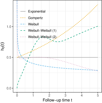
Figure 1: Baseline hazard functions.

Table 1: Parameters of data-generating baseline hazard functions

Baseline hazard function	Parameters
Exponential	$\lambda=0.5$
Weibull	$\lambda=0.5,p=0.8$
Gompertz	$\lambda=0.5,\gamma=0.2$
Weibull-Weibull (1)	$\lambda_{1}=0.3,\lambda_{2}=0.5,p_{1}=1.5,p_{2}=2.5,\pi=0.7$
Weibull-Weibull (2)	$\lambda_{1}=0.5,\lambda_{2}=0.5,p_{1}=1.3,p_{2}=0.7,\pi=0.5$

2.3 Estimands

The estimands of interest are estimates of relative risk, absolute risk, and heterogeneity. In addition, we monitor and report on convergence rates of each model as well.

Relative risk

The relative risk estimate of interest is the regression coefficient $\beta$ associated with the binary treatment; this coefficient can be interpreted as the log-treatment effect, conditional on the unobserved value of the frailty term. It is important to bear in mind therefore that the hazard ratio in a frailty model carries the usual interpretation only when comparing two hazards conditional on a given frailty; unconditionally, at a population level, the proportionality of hazards is not guaranteed to hold even under the proportional hazards parametrisation. For most frailty distributions (including the Gamma and log-Normal) the conditional hazard ratio is a true hazard ratio only at time $t=0$, as the effect of the covariates on the hazard varies over time depending on the actual distribution of the frailty ⁶, ⁸.

Absolute risk

The absolute risk estimate of interest is the 5-years loss in life expectancy (LLE) (associated with the treatment of interest), defined as the difference in life expectancy between exposed and non-exposed individuals. The marginal 5-years life expectancy (LE) for exposed individuals ($X=1$) is defined as

$$\text{LE}(X=1) =\int_{0}^{5}S(u|X=1)\ du$$

$$=\int_{0}^{5}\int_{A}S(u|X=1,\alpha)\ p(\alpha)\ d\alpha\ du,$$

where $A$ is the domain of the frailty $\alpha$ and $p(\alpha)$ its density function. Consequently, the LLE associated with not being exposed ($X=0$) compared with being exposed is defined as

$$\text{LLE}=\int_{0}^{5}S(u|X=1)\ du-\int_{0}^{5}S(u|X=0)\ du.$$

The inner integral in LE (i.e. $S(t|X=1)$) has a closed form when the frailty follows a Gamma distribution; with a log-Normal frailty (and with a mixture Normal frailty), numerical integration is required. We use the quadinf function from the pracma package in R to perform numerical integration, which implements the double exponential method for fast numerical integration of smooth real functions on finite intervals ³⁴. For infinite intervals, the tanh-sinh quadrature scheme is applied ³⁵. The outer integral in LE, however, is approximated using spline-based integration as follows. We first estimate LE over 1,000 values of $t$ between the minimum and the maximum observed survival times; then, we fit an interpolating natural spline function over the 1,000 LE estimates from step (1), which we finally integrate between 0 and 5 (years) using the double exponential method of quadinf. LLE follows by computing the difference between the two integrals. Finally, we computed the standard error of the estimated LLE using the numerical delta method (as implemented in the predictnl function from the rstpm2 R package).

Heterogeneity

With this simulation study we mainly focus on estimates of risk. Regardless, measures of heterogeneity are sometimes used to quantify dependence between clustered observations. Therefore, we reported the results of our simulations regarding the frailty variance in the Supporting Web Material only. As the frailty variance estimated by models assuming either a Gamma or a log-Normal distribution are not directly comparable (being modelled on different scales, hazard versus log-hazard), we do not include summary statistics for the frailty variance where the frailty distribution is misspecified.

2.4 Methods

A general shared frailty model, assuming proportional hazards, has the form

$$h(t_{ij}|X_{ij})=\alpha_{i}h_{0}(t_{ij})\exp(X_{ij}\beta)$$

when assuming a Gamma-distributed frailty with mean $1$ and variance $\theta$. $i$ indexes the cluster and $j$ indexes the individual. $t_{ij}$ and $X_{ij}$ are the survival time and covariates of the $j^{\text{th}}$ individual, $i^{\text{th}}$ cluster, respectively; $h(\cdot)$ is the hazard function, $h_{0}(\cdot)$ is the baseline hazard function, $\beta$ is a vector of regression coefficients, and $\alpha_{i}$ represent the frailty term. The frailty term is assumed to be independent of covariates. Conversely, with a log-Normal frailty, a general shared frailty model has the form

$$h(t_{ij}|X_{ij})=h_{0}(t_{ij})\exp(X_{ij}\beta+\eta_{i}),$$

with $\exp(\eta_{i})=\alpha_{i}$. $\eta_{i}$ is assumed to have a mean of $0$ and a variance of $\sigma^{2}$. The latter model has a convenient interpretation: $\eta_{i}$ can be thought of as a random, cluster-specific, intercept.

The conditional survival function from a frailty model is

$$S_{ij}(t|\alpha_{i})=S_{ij}(t)^{\alpha_{i}}.$$

In this setting, the cluster-specific contribution to the likelihood is obtained by calculating the cluster-specific likelihood conditional on the frailty, consequently integrating out the frailty itself:

$$L_{i}=\int_{A}L_{i}(\alpha_{i})f(\alpha_{i})\,d\alpha,$$

with $L_{i}(\alpha_{i})$ the cluster-specific contribution to the likelihood, conditional on the frailty. The cluster-specific contribution to the likelihood is

$$L_{i}(\alpha_{i})=\alpha_{i}^{D_{i}}\prod_{j=1}^{n_{i}}S_{ij}(t_{ij})^{\alpha_{i}}h_{ij}(t_{ij})^{d_{ij}},$$

with $D_{i}=\sum_{j=1}^{n_{i}}d_{ij}$. A closed form formula for $L_{i}$ can be obtained when the frailty follows a Gamma distribution, with further details provided elsewhere ⁸. Otherwise, assuming a log-Normal frailty, the likelihood is analytically intractable and requires numerical integration to be performed (using method such as adaptive Gauss-Hermite quadrature ³⁶). Consequently, it is important to bear in mind then that the performance of the model fitting procedure will depend on the quality of the approximation. For instance: methods that rely on Gaussian quadrature will require an adequate number of integration points to provide an accurate approximation, while Laplace approximation performs poorly with a small number of clusters.

We compare a variety of different shared frailty models within this simulation study. First, we fit semiparametric shared frailty models by leaving the baseline hazard function $h_{0}(t_{ij})$ unspecified and assuming either a Gamma or a log-Normal frailty (Model 1-2, denoted by Cox in plots). Second, we fit fully parametric survival models by assuming that the baseline hazard function follows an exponential, Weibull, or Gompertz distribution; we fit each of the three models assuming both a Gamma and a log-Normal frailty distribution (Model 3-8, denoted by Exp, Wei, and Gom). As a comparison, we fit the Weibull model with both Gamma and log-Normal frailties using the R package frailtypack as well (Model 17-18, denoted by FP(W)). Third, we fit Royston-Parmar flexible parametric survival models generalised by Liu et al. to account for clustered and correlated survival data ¹, ³⁷, ²¹. Using the generalised survival model formulation, the model is formulated as

$$S(t_{ij}|X_{ij},\alpha_{i})=\{G(\eta(t_{ij},X_{ij};\beta))\}^{\alpha_{i}},$$

with $G(\cdot)=g^{-1}(\cdot)$ an inverse link function and $\eta(\cdot)$ a linear predictor function of time and covariates. Choosing the log-log link function, the model is a proportional hazards model; modelling the log of time with natural splines, we obtain a Royston-Parmar model whose parameters can be fit using fully parametric maximum likelihood. We assume 3, 5, or 9 degrees of freedom for the natural spline of time and fit models using both Gamma and log-Normal shared frailties (Model 9-14, denoted by RP(df) where df is the number of degrees of freedom). In order to avoid choosing the number of degrees of freedom for the spline term, we estimate the same Royston-Parmar model with shared frailties using penalised likelihood ²¹ and either a Gamma or log-Normal frailty (Model 15-16, denoted by RP(P)). The penalty term accounts for the complexity of the smoother of time to avoid overfitting the data; however, additional computational complexity is required to select the smoothing parameter (or parameters). More details on the penalised marginal likelihood estimation procedure are provided in Liu et al. ²¹. Finally, we fit shared frailty models where the baseline hazard function is approximated by cubic M-splines on the hazard scale ³⁸; such models are fitted using penalised likelihood, and we fix the smoothing parameter $\kappa$ to the value 10 and 10000 as in the simulations of Liu et al. ²¹ (Model 19-22, denoted by FP(k=kappa), with kappa the smoothing parameter $\kappa$).

2.5 Performance measures

The first performance measure of interest is bias, quantifying whether an estimator targets the true value on average. Formally, it is defined as $E(\hat{\beta})-\beta$, with $\hat{\beta}$ estimates of the parameter $\beta$. Second, we are interested in coverage, i.e. the proportion of times the $100\times(1-\alpha)\%$ confidence interval $\hat{\beta}\pm Z_{1-\alpha/2}\times SE(\hat{\beta})$ includes the true value $\beta$. This allows assessing whether the empirical coverage rate approaches the nominal coverage rate ($100\times(1-\alpha)\%$). Finally, we are interested in mean squared error [MSE]; MSE is the sum of the squared bias and variance of $\hat{\beta}$ and represents a natural way to integrate both performance measures into one. However, the relative influence of bias and variance of $\hat{\beta}$ varies with the number of simulations making generalising results difficult. Further details on the performance measures of interest are given in Burton et al. ³⁹ and Morris et al. ⁴⁰. We also report on convergence rates for each model, and we include Monte Carlo standard errors for bias, coverage, and MSE to quantify the uncertainty in estimating such performance measures ⁴⁰, ⁴¹.

In order to avoid the inflation of summary statistics caused by software spuriously declaring convergence, we manually declared as non-converged all the model fits that returned standardised point estimates or standardised standard errors larger than 10 in absolute value. We standardised values using median and inter-quartile range for robustness.

2.6 Number of simulations

We generate $1,000$ simulated data sets for each scenario; with $1,000$ replications, assuming a variance of $0.1$ for the estimated bias, we expect a Monte Carlo standard error of $0.01$ for the estimated bias. Being bias the key performance measure of interest, we deemed this acceptable. Additionally, Monte Carlo standard error for coverage is maximised when coverage is $50\%$; with $1,000$ replications, the expected Monte Carlo standard error for coverage would be $1.58\%$. Should coverage be optimal at $95\%$, the expected Monte Carlo standard error would be $0.68\%$. We deemed the expected Monte Carlo standard error for coverage to be acceptable too.

2.7 Software

All models included and compared in this simulation study can be fitted using R and standard, freely available user-written packages. Furthermore, we did not tweak any of the convergence parameters utilised for declaring convergence of the estimation algorithm. The semiparametric shared frailty models can be fitted using the frailtyEM and coxme packages for a Gamma and log-Normal frailty, respectively. frailtyEM fits a Gamma frailty model using the expectation-maximisation [EM] algorithm ⁴², while coxme relies on penalised likelihood ⁴³. A comparison of R packages for fitting semiparametric frailty models is given in Hirsch and Wienke, 2012 ⁴⁴; other possible packages that support semiparametric shared frailty models (using different estimation algorithms) are frailtySurv ⁴⁵ and frailtyHL ⁴⁶. The fully parametric shared frailty models can be fitted using the parfm package for either a Gamma or a log-Normal frailty; models are fit using full likelihood, and Laplace integration is used when required ⁴⁷. The Weibull shared frailty model is also fit using the R package frailtypack for comparison (denoted by FP(W)). The flexible parametric models on the log-cumulative hazard scale with shared frailties can be fitted using the rstpm2 package. When specifying the number of degrees of freedom for modelling the baseline hazard full likelihood is used, otherwise rstpm2 relies on penalised likelihood estimation. The models with the baseline hazard function approximated by cubic M-splines on the hazard scale are fitted using the R package frailtypack.

All packages but coxme returned a standard error for the estimated frailty variance; therefore, when fitting a semiparametric shared frailty model with a log-Normal frailty, we bootstrapped the standard error of the frailty variance using 1,000 bootstrap replications and resampling at the cluster level to preserve the within-cluster correlation.

Finally, only frailtyEM, rstpm2, and frailtypack provided a function to predict marginal survival; for coxme and parfm, we manually wrote ad-hoc R functions to estimate marginal survival, using numerical integration when required.

All the R code utilised to simulate clustered survival data and fit each model from this simulation study is freely and openly available online on Github: https://github.com/ellessenne/frailtymcsim; we denote the version of each package used for our simulations in Table 2.

Table 2: Version of each R package used for our simulations

R Package	Version
frailtyEM	0.8.8
coxme	2.2-10
parfm	2.7.6
frailtypack	3.0.2.1
rstpm2	1.4.5

3 Results

Among the 90 simulated scenarios, we select a subset of them to focus on for conciseness; specifically, we select all scenarios with 20 clusters of 150 individuals each. This adds up to 45 simulated scenarios, and results for the remaining 45 scenarios (with 750 clusters of 2 individuals each) are included in the Supporting Web Material available online from the aforementioned GitHub repository (https://github.com/ellessenne/frailtymcsim).

The full results of the simulation study and the summary statistics can be downloaded as well from the same GitHub repository, where we included the full results tabulated by estimand and data-generating scenario and additional plots. We recommend downloading the full dataset and exploring results interactively using the web app INTEREST, available online at https://interest.shinyapps.io/interest/ and as a stand-alone, offline package at https://github.com/ellessenne/interest.

3.1 Convergence rates

Convergence rates were good for most models and most scenarios, with 75% of model – scenarios combinations showing a convergence rate of 98.5% or above (Figure 2). However, some exceptions could be found:

1. Parametric models with a Gompertz baseline hazard had the worst convergence rates, with a median convergence rate of 43.20% (inter-quartile range: 29.25% – 55.85%);

2. Parametric models with a Weibull baseline hazard and a log-Normal frailty fitted using the frailtypack package caused R to hang indefinitely in several scenarios, yielding a median convergence rate of 81.00% (inter-quartile range: 65.30% – 97.30%);

3. frailtypack models with a smooth baseline hazard modelled using M-splines showed low convergence rates for other scenarios as well, especially when simulating heterogeneity from a mixture Normal frailty distribution;

4. Some frailtypack models and some parametric models with a Gompertz baseline hazard did not converge at all in some scenarios with simulated data assuming a mixture Normal frailty;

5. All convergence rates are depicted in Online Web Figure 7, available in the Supporting Web Material.

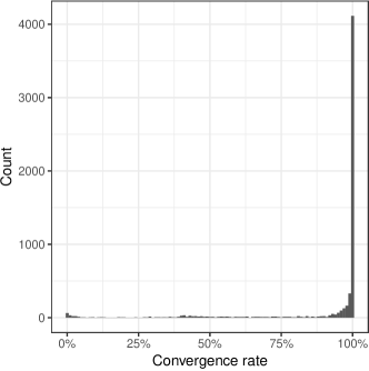
Figure 2: Histogram of convergence rates per each model – scenario combination.

Furthermore, Online Web Figure 8 depicts predicted marginal probabilities of non-convergence; the Gompertz models, the Weibull model with a log-Normal frailty from frailtypack, and the model with M-splines, a smoothing parameter $k=10000$, and a Gamma frailty showed the highest predicted probabilities of non-convergence, all else being equal. The probability of non-convergence also increased alongside the variance of the frailty, and when simulating from a log-Normal or mixture Normal (compared to a Gamma) distribution. Finally, Online Web Figure 9 depicts the proportion of non-converged scenarios against the average proportion of observed events per simulated scenario and model included in our comparison. Models with worse convergence rates showed an association between non-convergence and the average proportion of events, with stronger right censoring being associated with worse convergence rates. Ultimately, the factors that seemed to be associated with convergence rates were the censoring proportion, the variance of the frailty, and the distribution of the frailty. Nevertheless, the software implementation and the algorithms used for fitting each model seem to play an important role, with some software implementations being more robust than others to variations in the factors outlined before.

3.2 Results for the regression coefficient

Bias, coverage, and MSE of the regression coefficient for the scenarios with 20 clusters of 150 individuals each are presented in Figures 3, 4, and 5. With a simple, exponential true baseline hazard all models performed equally well in terms of bias and coverage. Conversely, assuming a too simple parametric distribution with a more complex true baseline hazard (or misspecifying the baseline hazard) yielded a biased regression coefficient: significant positive bias up to 0.175 and negative bias up to -0.105 for the models assuming an exponential baseline hazard, and analogously for the models assuming a Gompertz baseline hazard with positive bias up to 0.171 and negative bias up to -0.112. A positive bias of 0.175 on the log-hazard ratio scale corresponds to a 19% relative risk overestimation; a negative bias of -0.112 corresponds to a 11% relative risk underestimation. The semiparametric Cox models and all the flexible parametric models (irrespectively of the number of degrees of freedom employed and of the estimation procedure) yielded unbiased results, with the exception of the model with 9 degrees of freedom when the true frailty followed a mixture Normal distribution with component-specific variances of 1.25. In that setting and assuming a Weibull and a mixture Weibull (2) true baseline hazard the flexible parametric model yielded large biases - although this seems to be a somewhat spurious result given the performance of the same method in other scenarios. All models using M-splines on the hazard scale performed similarly to the parametric Weibull, with little to no bias; however, the performance of models using M-splines worsened with a true mixture Normal frailty distribution. Coverage was optimal for all models producing unbiased estimates; however, coverage dropped considerably for models that yielded biased estimates with coverage values as low as 5% for models showing the largest bias. Interestingly, misspecification of the frailty distribution did not affect much the pattern of results; despite that, bias seemed to worsen when we simulated the frailty from a log-Normal or mixture Normal distribution compared to a Gamma distribution, exacerbating the effect of misspecifying the baseline hazard. Finally, the models that showed the lowest MSE were the semiparametric models, the flexible parametric models, and the models using M-splines - irrespectively of the true baseline hazard and distribution of the frailty. The exponential and Gompertz parametric models showed a larger MSE - up to 10-fold larger - when the baseline hazard was misspecified, with the Gompertz model showing an MSE larger than semiparametric and flexible parametric models even when well specified. The Weibull model, as observed before, performed similarly to semiparametric and flexible parametric models. Finally, this pattern of results was largely maintained with the remaining scenarios (with 750 clusters of 2 individuals each); the corresponding plots are included in the Supporting Web Material.

3.3 Results for the 5-years LLE

Bias, coverage, and MSE for the 5-years LLE are presented in Figures 6, 7, and 8, respectively. The pattern we observed for LLE mirrors the pattern observed for the regression coefficient: models with a misspecified baseline hazard (or a baseline hazard not flexible enough to capture the underlying shape) yielded biased results, both positive and negative. Negative bias was up to -0.057 and positive bias was up to 0.031: this corresponds, respectively, to a difference of approximately (minus) 1 month and half a month in the estimated LLE. The Weibull model fit with frailtypack largely underestimated the 5-years LLE in all scenarios (negative bias between -0.184 and -0.100), and the M-splines model with smoothing parameter $\kappa=10000$ and a Gamma distribution performed even worse when the true baseline hazard followed a Weibull-Weibull (1) distribution (negative bias between -0.461 and -0.169). The large bias observed for this M-splines model in these scenarios seems to be spurious - analogously as before with the flexible parametric model. Interestingly, models with a well-specified frailty performed better than models with a misspecified frailty, both for a true Gamma and log-Normal frailty. Conversely, when simulating from a mixture Normal distribution all models yielded positively biased results (up to 0.257, e.g. 3 months) with exceptions being the frailtypack models described before, where underestimation of the results still applied. Coverage followed a similar pattern, with optimal coverage for models with small bias and reduced coverage for models that yielded biased results; overall, coverage was better when the frailty distribution was well specified. As a consequence of the large positive bias, coverage in scenarios simulated from a mixture Normal distribution was poor. Mean squared error was similar across all scenarios with minimal variability and a notable exception: models fitted using M-splines for the baseline hazard and a log-Normal frailty had a much higher MSE, approximately 10 times larger. Another interesting observation is that the empirical standard error (the standard deviation of the estimated LLE) was systematically larger than the mean of the standard errors for LLE obtained using the numerical delta method (results included in the Supporting Web Material; we can conclude that the numerical delta method used to obtain a standard error for LLE underestimated the standard error. Finally, once again results for the remaining scenarios (included in the Supporting Web Material) are similar to the results presented in the main body of the manuscript.

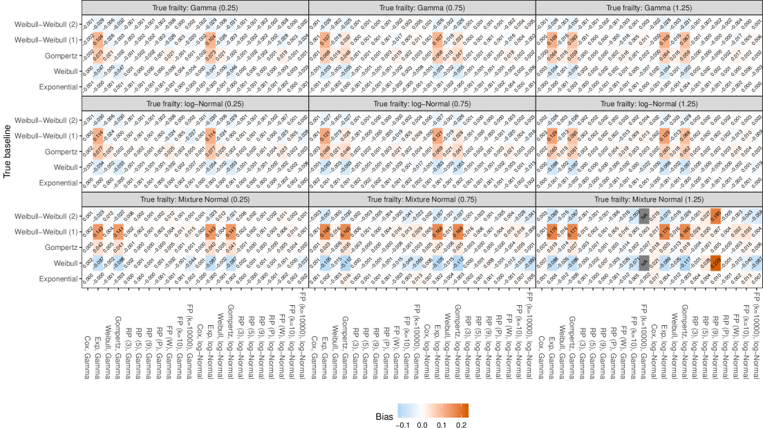
Figure 3: Bias of regression coefficient, scenario: 20 clusters of 150 individuals each. Colours represent positive and negative bias, and solid grey represents scenarios where no model converged.

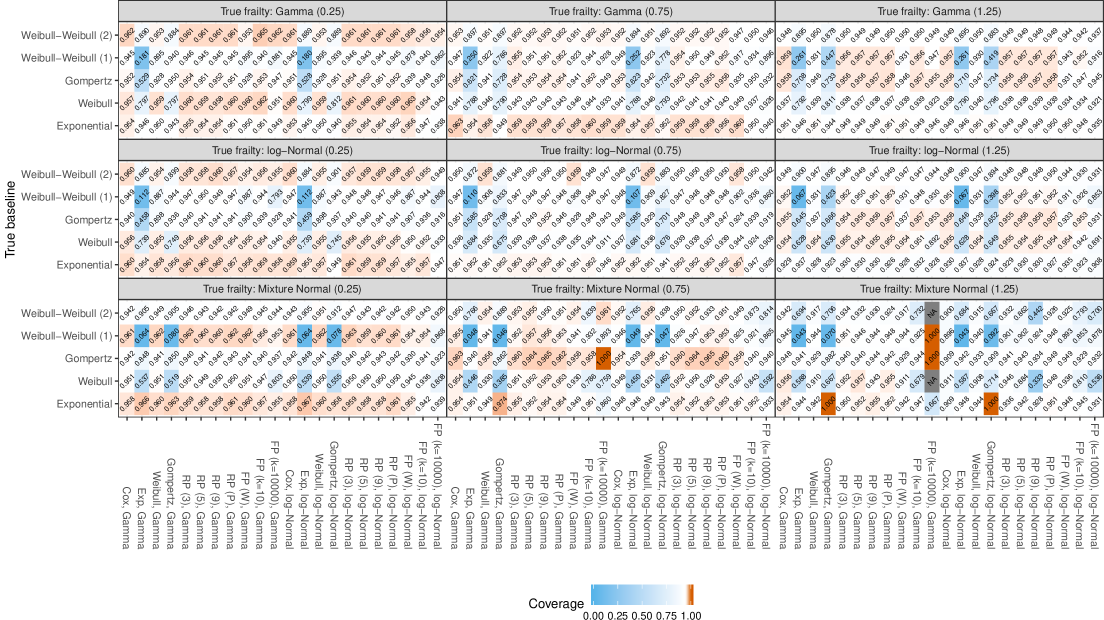
Figure 4: Coverage of regression coefficient, scenario: 20 clusters of 150 individuals each. Colours represent positive and negative bias, and solid grey represents scenarios where no model converged.

Figure 5: Mean squared error of regression coefficient, scenario: 20 clusters of 150 individuals each. Colours represent positive and negative bias, and solid grey represents scenarios where no model converged.

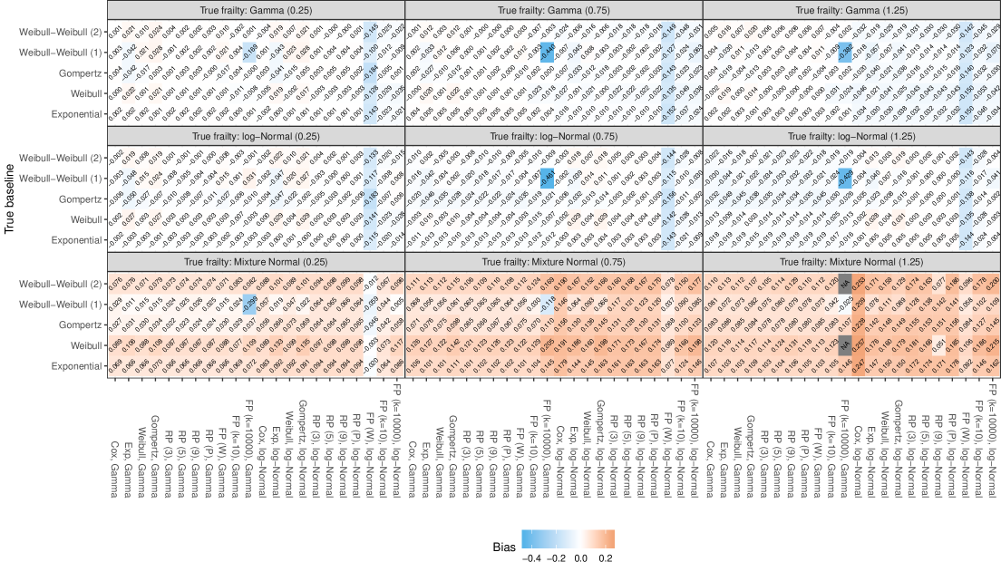
Figure 6: Bias of LLE, scenario: 20 clusters of 150 individuals each. Colours represent positive and negative bias, and solid grey represents scenarios where no model converged.

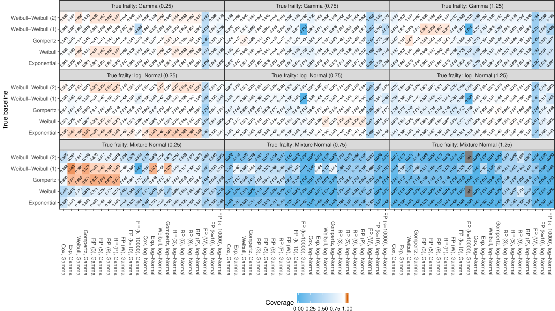
Figure 7: Coverage of LLE, scenario: 20 clusters of 150 individuals each. Colours represent positive and negative bias, and solid grey represents scenarios where no model converged.

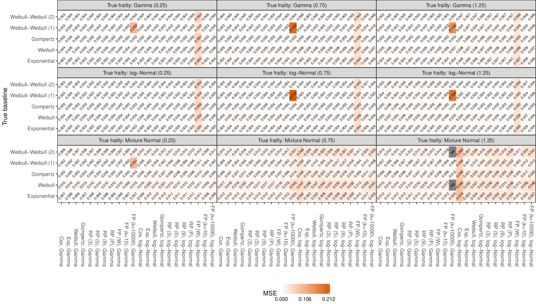
Figure 8: Mean squared error of LLE, scenario: 20 clusters of 150 individuals each. Colours represent positive and negative bias, and solid grey represents scenarios where no model converged.

4 Application to diabetic retinopathy data

In this section, we apply the models included in our simulation study to a dataset from the Diabetic Retinopathy Study. The outcome of interest here is time to blindness, and we include laser treatment as a binary covariate. Laser treatment is the main exposure of interest, and we do not include other covariates for simplicity. We define the subject ID as the cluster indicator variable to account for correlation between eyes of a given individual, and we aim to present estimates of treatment effect and five-years LLE. The model we fit is a model of the kind:

$$h(t_{ij})=\alpha_{i}h_{0}(t_{ij})\exp(X_{ij}\beta),$$

with $i$ and $j$ being the individual-level and eye-level indicator variables, $t_{ij}$ the time to event for eye $j$ of individual $i$, $\beta$ being the treatment effect, $X_{ij}$ the treatment modality for eye $j$ of individual $i$, and $\alpha_{i}$ the frailty for individual $i$. We model the baseline hazard $h_{0}(\cdot)$ via fully parametric and flexible parametric distributions or by leaving it unspecified. The flexible parametric models are modelled on the log-cumulative hazard scale:

$$\log H(t_{ij})=s(\log(t_{ij})|\gamma,k_{0})+X_{ij}\beta+\eta_{i},$$

with $s(\cdot)$ a spline function of log-time with parameter vector $\gamma$ and knot vector $k_{0}$. Despite being on the log-cumulative hazard scale, the aforementioned model is still a proportional hazards model. Finally, we model the frailty distribution assuming either a Gamma or log-Normal distribution.

The dataset consisted of 394 observation clustered in 197 patients; the median follow-up, estimated using the inverse Kaplan-Meier method ⁴⁸ and using robust standard errors to account for clustering, was 51.10 months, with a confidence interval (based on the estimated survival curve) of 47.60 to 54.37 months.

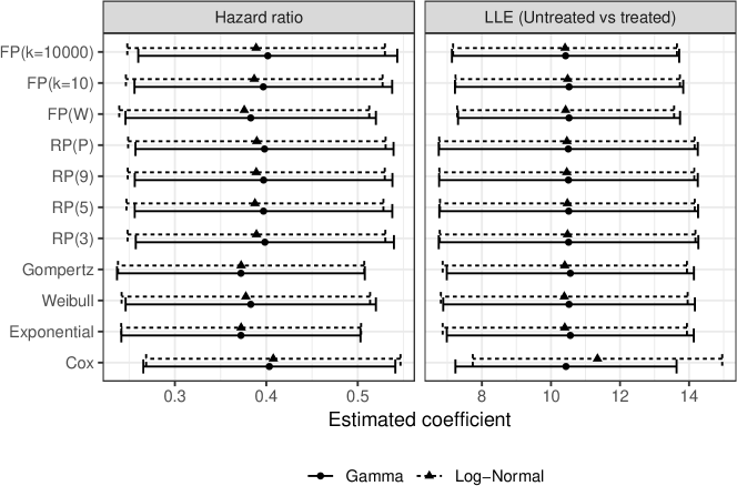
Figure 9: Comparison of relative and absolute estimates of risk with confidence intervals, application to diabetic retinopathy data

Table 3: Results: application of shared frailty models to a subset of data from the DRS. Values in rounded brackets are standard errors for each estimate.

Baseline	Hazard ratio	Frailty variance	LLE (Untreated vs treated)
Gamma frailty:
Cox	0.4033 (0.0703)	0.8477 (0.3140)	10.4346 (1.6335)
Exponential	0.3723 (0.0667)	1.1490 (0.3028)	10.5606 (1.8244)
Weibull	0.3830 (0.0698)	1.0402 (0.3293)	10.5231 (1.8585)
Gompertz	0.3723 (0.0691)	1.1490 (0.3516)	10.5606 (1.8253)
RP(3)	0.3985 (0.0720)	0.8875 (0.3185)	10.5104 (1.9171)
RP(5)	0.3969 (0.0718)	0.9067 (0.3215)	10.5140 (1.9117)
RP(9)	0.3970 (0.0718)	0.9046 (0.3208)	10.5057 (1.9104)
RP(P)	0.3981 (0.0720)	0.8943 (0.3195)	10.5016 (1.9138)
FP(W)	0.3830 (0.0698)	1.0402 (0.3294)	10.5232 (1.6393)
FP(k=10)	0.3967 (0.0719)	0.9036 (0.3217)	10.5241 (1.6857)
FP(k=10000)	0.4016 (0.0722)	0.8751 (0.3146)	10.4233 (1.6790)
Log-normal frailty:
Cox	0.4076 (0.0709)	0.7771 (0.2990)	11.3468 (1.8417)
Exponential	0.3725 (0.0669)	1.2183 (0.3054)	10.4002 (1.8043)
Weibull	0.3776 (0.0693)	1.1594 (0.3379)	10.3862 (1.8232)
Gompertz	0.3725 (0.0687)	1.2183 (0.3487)	10.4001 (1.8046)
RP(3)	0.3892 (0.0719)	1.0287 (0.3861)	10.4800 (1.8889)
RP(5)	0.3876 (0.0717)	1.0560 (0.3916)	10.4747 (1.8818)
RP(9)	0.3890 (0.0717)	1.0362 (0.3849)	10.4579 (1.8833)
RP(P)	0.3896 (0.0718)	1.0270 (0.3839)	10.4617 (1.8863)
FP(W)	0.3759 (0.0697)	1.1967 (0.4023)	10.4241 (1.6023)
FP(k=10)	0.3868 (0.0716)	1.0621 (0.3919)	10.4838 (1.6575)
FP(k=10000)	0.3889 (0.0719)	1.0623 (0.3934)	10.4080 (1.6536)

We first fit all the models without including any other covariate than the exposure to treatment; results are presented in Figure 9 and Table 3. The log-treatment effect varied between -0.9882 and -0.8974, corresponding to hazard ratios of 0.3723 to 0.4076, respectively. Analogously, the estimates of 5-years LLE ranged between 10.3862 and 11.3468 months for non-exposed compared to exposed. LLE can be interpreted as follows: on average, individuals not treated with laser experienced blindness approximately 11 months before individuals that received the treatment. The difference in estimated risk (relative and absolute) appears to be relevant, highlighting once again the importance of choosing an appropriate functional form of the baseline hazard.

Table 4: Results: comparison of AIC/BIC from shared frailty models, application to a subset of data from the DRS. Best AIC/BIC values are in bold.

Baseline	AIC	BIC
Gamma frailty:
Cox	—	1 —
Exponential	1,661.96	1,673.89
Weibull	1,663.49	1,679.39
Gompertz	1,663.96	1,679.87
RP(3)	1,663.11	1,686.97
RP(5)	1,665.08	1,696.90
RP(9)	1,659.40	1,707.12
RP(P)	—	1 —
FP(W)	1,663.49	1,679.39
FP(k=10)	—	1 —
FP(k=10000)	—	1 —
Log-normal frailty:
Cox	—	—
Exponential	1,656.99	1,668.92
Weibull	1,658.87	1,674.78
Gompertz	1,658.99	1,674.89
RP(3)	1,662.01	1,685.87
RP(5)	1,663.90	1,695.71
RP(9)	1,658.37	1,706.09
RP(P)	—	—
FP(W)	1,662.27	1,678.17
FP(k=10)	—	—
FP(k=10000)	—	—

In Table 4 we present AIC and BIC for the models fitted using full likelihood on DRS data; the best model according to each criterion is highlighted in bold. We do not include models fitted using either partial or penalised likelihood in this comparison. The best model according to both the AIC and the BIC is the model with a log-Normal frailty and an exponential baseline hazard; however, a non-parametrical estimate of the hazard function using a kernel-based method (Figure 10, R package bshazard) seems to suggest against assuming an exponential baseline hazard function. Therefore, we select the second-best model in terms of AIC as the model we focus on, that is, the flexible parametric model with the baseline hazard modelled via a restricted cubic spline with 9 degrees of freedom and a log-Normal frailty. The penalised model with a flexible parametric baseline hazard and a log-Normal frailty selected an effective number of degrees of freedom of 9.6261, very similar to the final model we selected. However, it is important to remember that other information criteria are available, especially for models with random effects. Vaida and Blanchard ⁴⁹ suggested the use of conditional AIC (cAIC) for model selection in linear mixed models. They demonstrated that a classical AIC (i.e. marginal AIC) and its small sample correction are inappropriate when the interest is on cluster: see also Liang, Wu and Zou ⁵⁰. Unfortunately, the cAIC is not routinely reported by software fitting shared frailty models (with the exception of frailtyHL ⁵¹, ⁴⁶). We encourage the maintainers of such R packages to add it to their packages, enabling applied researchers to use information criteria for model selection that are more appropriate in the settings of random effects models. Using the flexible parametric approach, it is straightforward to model the baseline hazard function in continuous time and it is possible to obtain smooth predictions. It is also straightforward to accommodate time-varying covariates effects (and therefore assess the proportional hazards assumption), as we demonstrate next.

Figure 10: Smooth non-parametric hazard estimate, overall and by treatment modality.

Figure 11: Marginal hazard ratio (A) and marginal survival difference (B), comparing a flexible parametric model with 9 degrees of freedom and a log-Normal frailty with and without a time-dependent treatment effect. Application to diabetic retinopathy data.

We include in flexible parametric model identified by the AIC as the second best an interaction between treatment and the natural logarithm of time, modelled using a natural spline:

$$\log H(t_{ij})=s(\log(t_{ij})|\gamma,k_{0})+X_{ij}\beta+s(\log(t_{ij})|\delta,l_{0})X_{ij}+\eta_{i},$$

with the treatment variable $X_{ij}$ is interacted with a spline function of log-time with associated coefficient vector $\delta$ and knots vector $l_{0}$. Flexible parametric models have been showed to be insensitive to the number of knots utilised to model time-varying effects, therefore we choose to use 3 degrees of freedom for simplicity ⁵². The difference between the marginal hazard ratio estimated using the model with a time-dependent treatment effect and the model without is depicted in Figure 11, panel A. The difference seems to be larger early on in the study, attenuating as time goes by. As a comparison, we also include the marginal survival difference between treated and untreated individuals, estimated assuming both time-fixed and time-varying effects (Figure 11, panel B). Finally, we test whether the time-treatment interaction is statistically significant using a likelihood ratio test. We obtain a $\chi^{2}$ test statistic of 2.87 and a p-value of 0.41: this suggest that there is not enough evidence to support the presence of a time-dependent treatment effect.

5 Application to bladder cancer data

We also apply the same models from our simulation study to a dataset constructed by pooling 7 trials on bladder cancer comparing chemotherapy against no chemotherapy. The outcome of interest is time from randomisation to cancer relapse, in years; patients still alive and without recurrence were censored at the date of the last available follow-up cystoscopy. We then compare estimates of relative and absolute risk; specifically, we compare the hazard ratio and the 1-year LLE of chemotherapy against no chemotherapy, respectively.

The dataset included 410 patients from 21 unique centres that participated in EORTC trials. The median follow-up, estimated once again using the inverse Kaplan-Meier method ⁴⁸ and assuming robust standard errors was 3.52 years (confidence interval: 3.28 – 3.88). The minimum and maximum observed follow-up times are 1 day and 10.15 years, respectively.

Figure 12: Comparison of relative and absolute estimates of risk, application to bladder cancer data

Table 5: Results: application of shared frailty models fitted to the bladder cancer data.

Baseline	Hazard ratio	Frailty variance	LLE (Untreated vs treated)
Gamma frailty:
Cox	0.5056 (0.0880)	0.0468 (0.0484)	0.1235 (0.0249)
Exponential	0.4601 (0.0812)	0.0755 (0.0617)	0.1118 (0.0320)
Weibull	0.4895 (0.0860)	0.0558 (0.0525)	0.1210 (0.0358)
Gompertz	0.4601 (0.0815)	0.0755 (0.0620)	0.1118 (0.0321)
RP(3)	0.4997 (0.0876)	0.0524 (0.0506)	0.1269 (0.0369)
RP(5)	0.5000 (0.0876)	0.0522 (0.0500)	0.1262 (0.0369)
RP(9)	0.5014 (0.0878)	0.0510 (0.0497)	0.1250 (0.0367)
RP(P)	0.5046 (0.0883)	0.0478 (0.0488)	0.1242 (0.0367)
FP(W)	0.4895 (0.0860)	0.0558 (0.0525)	0.1210 (0.0226)
FP(k=10)	0.5340 (0.0941)	0.0416 (0.0457)	0.1132 (0.0253)
FP(k=10000)	0.4910 (0.0768)	0.0610 (0.0526)	0.1129 (0.0188)
Log-normal frailty:
Cox	0.5023 (0.0877)	0.0640 (0.0593)	0.1268 (0.0255)
Exponential	0.4586 (0.0810)	0.0891 (0.0744)	0.1131 (0.0323)
Weibull	0.4881 (0.0858)	0.0634 (0.0608)	0.1219 (0.0360)
Gompertz	0.4586 (0.0813)	0.0891 (0.0748)	0.1131 (0.0324)
RP(3)	0.4983 (0.0874)	0.0591 (0.0580)	0.1276 (0.0370)
RP(5)	0.4988 (0.0874)	0.0583 (0.0568)	0.1269 (0.0370)
RP(9)	0.5001 (0.0877)	0.0570 (0.0564)	0.1257 (0.0368)
RP(P)	0.5034 (0.0882)	0.0534 (0.0553)	0.1249 (0.0368)
FP(W)	0.4818 (0.0844)	0.0787 (0.0585)	0.1279 (0.0233)
FP(k=10)	0.5169 (0.0915)	0.0826 (0.0473)	0.1254 (0.0268)
FP(k=10000)	0.4760 (0.0743)	0.1046 (0.0635)	0.1263 (0.0202)

Estimates values from each model fitted to the bladder trial data are presented in Table 5 and Figure 12. The estimated treatment effect obtained from the semiparametric models and the flexible parametric models are practically overlapping, with an hazard ratio of approximately $0.50$ (range: 0.4983 to 0.5056). Conversely, the parametric models returned different results: the estimated relative risk was $2-4\%$ lower (e.g. hinting towards a greater benefit of chemotherapy). Finally, the penalised model fitted using the frailtypack package returned quite different results depending on the penalisation parameter $\kappa$, with hazard ratios ranging between 0.4760 and 0.5340 (approximately 6% risk difference), highlighting the importance of choosing an appropriate smoothing parameter. Analogously, the estimates of 1-year LLE were pretty consistent with each other and the semiparametric and flexible model estimates were the most similar. Among parametric models, the model with a Weibull baseline hazard seemed the most similar to semiparametric and flexible parametric models; the exponential and Gompertz models differed more, while penalised models from frailtypack returned estimates close to those of flexible parametric models (especially when assuming a log-Normal distribution for the frailty). Overall, the 1-year LLE comparing unexposed and exposed individuals varied between 0.1118 and 0.1279: practically speaking, on average, individuals not exposed to chemotherapy experienced recurrence of bladder cancer 1-1.5 months earlier during the first year of follow-up.

Table 6: Results: comparison of AIC/BIC from shared frailty models, application to bladder cancer data. Best AIC/BIC values are in bold.

Baseline	AIC	BIC
Gamma frailty:
Cox	—	1 —
Exponential	959.57	971.62
Weibull	951.45	967.52
Gompertz	961.57	977.63
RP(3)	884.69	908.78
RP(5)	864.67	896.80
RP(9)	858.16	906.36
RP(P)	—	1 —
FP(W)	951.45	967.52
FP(k=10)	—	1 —
FP(k=10000)	—	1 —
Log-normal frailty:
Cox	—	—
Exponential	959.36	971.41
Weibull	951.35	967.42
Gompertz	961.36	977.43
RP(3)	884.59	908.69
RP(5)	864.59	896.72
RP(9)	858.08	906.28
RP(P)	—	—
FP(W)	951.66	967.72
FP(k=10)	—	—
FP(k=10000)	—	—

Comparing model fit using AIC and BIC, the model with a flexible baseline hazard provided the best fit according to both AIC and BIC. Specifically, the model with 5 degrees of freedom for modelling the baseline hazard and a log-Normal frailty was selected as the best model by BIC. The penalised model with a flexible parametric baseline hazard and a log-Normal frailty selected an effective number of degrees of freedom of 11.75. Utilising this model to predict the marginal hazard, we obtained Figure 13: first, individuals not exposed to chemotherapy showed a higher hazard; second, we observed that the hazard spiked early on and then decayed over time.

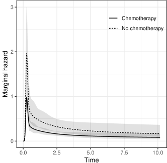
Figure 13: Marginal hazard estimated from the flexible parametric model with 5 degrees of freedom and a log-Normal frailty. Application to bladder cancer data.

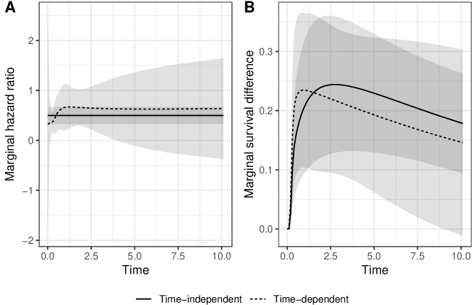
Figure 14: Marginal hazard ratio (A) and marginal survival difference (B), comparing a flexible parametric model with 5 degrees of freedom and a log-Normal frailty with and without a time-dependent treatment effect. Application to bladder cancer data.

Finally, analogously as the diabetic retinopathy applied example, it is possible to test for a time-dependent effect of chemotherapy. We utilise once again a natural spline with 3 degrees of freedom to model the interaction between the logarithm of time and chemotherapy. The estimated marginal hazard ratio and survival difference with and without assuming a time-dependent treatment effect are presented in Figure 14. The lines with estimated hazard ratios cross at approximately 6 months of follow up: this showed a greater estimated benefit of chemotherapy early on that lowers over time until it converges to a risk reduction of approximately a $30\%$ if we assume the effect of chemotherapy to be time-dependent; conversely, the risk reduction when assuming time-independent effects is approximately $50\%$. The same pattern can be observed with the marginal survival difference. Finally, we can test the significance of the time-treatment interaction using the likelihood ratio test: if we do so, we obtain a $\chi^{s}$ test statistic of 2.44 and a p-value of 0.49 – evidence against the presence of a time-dependent effect of chemotherapy.

6 Discussion

In observational studies and clinical trials with survival outcomes and an intrinsic hierarchical structure, survival models with shared frailty terms and/or random effects have moved from being a speciality rarely used that requires ad hoc software to being mainstream methods that can be utilised with any general-purpose statistical software such as R and Stata. Compared to a marginal approach (i.e. accounting for clustering by using a robust estimator of the variance-covariance matrix of the estimated coefficients), the frailty approach allows focussing on inference within the clusters and quantifying the amount of heterogeneity between clusters by directly modelling it. Additionally, the frailty approach can be used to model recurrent events data, assuming that the recurrent event times are independent conditional on the covariates and random effects ⁵³, ⁵⁴. Consequently, the adoption and use of such models have been steadily increasing in all fields of application: for instance, psychiatry ⁵⁵, orthodontia ⁵⁶, diabetes ⁵⁷, healthcare research ⁵⁸, leukaemia ⁵⁹. It is also increasingly common to encounter survival data with some sort of hierarchical structure; for instance, multi-centre clinical trials and individual patient data meta-analysis, twin studies, paired organs studies, and observational studies with geographical clustering. Another relevant source of hierarchical data is electronic health records, where individuals can be clustered within e.g. primary care practice.

Glidden and Vittinghoff ¹⁹ showed the benefit of using frailty models instead of models with fixed effects only or stratified approaches in the setting of multi-centre clinical trials, which may have driven adoption and use. Despite the increasing use of such methods, however, there has been little research on the impact of violating modelling assumptions - especially regarding the shape of the baseline hazard. Much research has focussed on misspecification of the frailty distribution, and the consensus is that relative risk estimates are largely unaffected by it ¹⁸, ¹⁹, ²⁰, ²¹. However, little is known about the impact of misspecifying the frailty on measures of absolute risk. With this simulation study, we aimed to shed further light on the topic and ultimately provide additional guidance to applied researchers.

We simulated clustered survival data under a variety of clinically plausible scenarios, assuming different shapes for the baseline hazard function and different distributions for the shared frailty. We varied the amount of heterogeneity in the data we simulated, and we also varied sample size, both in terms of number of clusters and number of individuals per cluster. We then fitted a large variety of survival models with shared frailty terms: assuming standard parametric distributions for the baseline hazard, modelling the baseline hazard in a flexible way via restricted cubic splines, and also leaving the baseline hazard unspecified. Each model was fit assuming both a Gamma and a log-Normal distribution for the frailty, arguably the most common choices in literature: the Gamma frailty has convenient mathematical features and it is analytically tractable, while the log-Normal frailty has a direct interpretation as a random intercept in a multilevel mixed-effects survival model. To the best of our knowledge, this is the most extensive simulation study on the impact of misspecifying the baseline hazard, the frailty distribution, or both in shared frailty survival models: Rutherford et al. only studied the robustness of flexible parametric models and did not consider frailty terms, while Pickles and Crouchley, Glidden and Vittinghoff, and Lee and Thompson only studied misspecification of the random effects distribution ², ¹⁸, ¹⁹, ²⁰. Liu et al. focussed on generalised survival model ²¹, and Ha et al. studied both misspecification of the baseline hazard and the frailty distribution but included fewer models in their comparison and only simulated a small amount of scenarios ²².

The results of our extensive simulations confirm the robustness of regression coefficients to misspecification of the frailty distribution, irrespectively of sample size and amount of heterogeneity in the data. However, our results also show the importance of modelling the baseline hazard in a satisfactory way. For instance, as we showed in Section 3, the bias induced by assuming a standard parametric distribution with a true complex baseline hazard can be clinically relevant. In practical terms, this means that by failing to model the baseline hazard we could be largely overestimating (or underestimating) the effect of interest. In the applied examples of Sections 4 and 5, the estimates of relative risk differ by 3-6% between the models - a difference that can be significant in clinical terms. We showed that absolute measures of risk such as the loss in expectation of life are affected by misspecification of both the baseline hazard and the frailty distribution: assuming a baseline hazard that is too simple or misspecifying the frailty distribution yields biased estimates and larger mean squared errors compared to well-specified models. In our applied examples, the difference in estimated LLE between models varied between 1 month (over 5 years) for the diabetic retinopathy example and 1-1.5 months (over 1 year) for the bladder cancer example. This highlights once again the necessity of using models that are flexible enough and the importance of assessing model fit regarding the distribution of the frailty by using information criteria such as the AIC and the BIC if no previous biological knowledge is available. In addition to that, we once again encourage the maintainers of software packages that can be used to fit shared frailty models to implement additional information criteria adjusted to account for the presence of the random effects, such as the cAIC ⁶⁰, ⁶¹. Comparing semiparametric Cox models and flexible parametric models, they produce unbiased relative risk estimates under any of the scenarios explored with this simulation study. However, the necessity of estimating the baseline hazard (e.g. by using the Breslow estimator) heavily affects the usage of semiparametric models when absolute risk measures are of interest. The Cox model is, de facto, the standard model fitted by applied researchers when dealing with time to event data; despite that, Sir David Cox himself argued in favour of parametric models ⁶², especially when interested in predicting the outcome for a given individual; parametric models are indeed known to have desirable features in terms of prediction, extrapolation, quantification of absolute risk measures. Flexible parametric models represent an attractive alternative to semiparametric and fully parametric survival models: they retain both the robustness to misspecification of the baseline hazard and the appealing advantages of parametric models for prediction, extrapolation, quantification. Since their introduction by Royston and Parmar ¹ in 2002, flexible parametric models have entered the statistical mainstream and have been extended to accommodate (among other) relative survival ⁶³, random effects ¹⁶, ²¹, and generalised link functions ³⁷. The advantage given to flexible parametric models versus semiparametric models by modelling the baseline hazard is particularly noteworthy: this allows translating relative risk measures on the absolute scale, aiding interpretation. With the two applications in Sections 4 and 5 we illustrate in practice the importance of choosing the right model, and how results are affected when that does not happen - with clinically relevant differences in risk estimates. Flexible parametric models produced consistent estimates, irrespectively of the number of degrees of freedom used to model the baseline hazard; this is consistent with previous results ², ⁵² and it is a key feature of this class of models.

We mentioned in Section 2.2 that we simulated and explored 90 distinct data-generating mechanisms: this wide variety is one of the advantages of this simulation study. Other advantages are: we included the most common frailty distributions (Gamma and log-Normal), and we simulated survival data under many different and clinically plausible baseline hazards. For instance, should we only simulate from a Weibull model, we would be assuming a baseline hazard that increases or decreased monotonically. While such an assumption could be reasonable in some settings, sometimes fully parametric distributions are just not flexible enough to capture complex baseline hazards with turning points that are often observed in clinical datasets ², ³³. This simulation study has also some limitations. First, we only simulated clusters of equal size and we did not include all the frailty distributions that have been proposed in the literature. Second, we simulated only right censored survival data; settings with delayed entry or interval censoring require further investigation. Third, all methods use maximum likelihood which returns negatively biased estimates of the variance components; such bias decreases as the number of clusters increases. The restricted maximum likelihood method could be used with a small number of clusters to obtain unbiased estimates of the variance components ⁶⁴. However, but the comparison between maximum likelihood and restricted maximum likelihood is outside of the scope of this manuscript. Fourth, we designed and analysed this simulation study using a fully factorial design; even though we simulated a large number of scenarios, incomplete designs and meta-modelling could be implemented to further increase the external validity and the ability to generalise our results, as described elsewhere ⁶⁵. Finally, we heavily rely on the performances and R implementation of the models we fit and compare; Hirsch and Wienke ⁴⁴ compared several implementations of the semiparametric Cox model with frailty terms and found coxme (our R package of choice for a semiparametric log-Normal frailty model) to be among the most robust. Regardless, all the packages we chose are well established and utilised in practice, and we mimicked applied research by applying these methods as they are intended to be used, i.e. without modifying convergence criteria and/or starting values of the estimation procedure.

7 Acknowledgements

MSC is supported by the Swedish eScience Research Centre. KRA is partially supported by the UK National Institute for Health Research (NIHR) as a Senior Investigator Emeritus (NF-SI-0512-10159). MJC is partially funded by a Medical Research Council (MRC) New Investigator Research Grant (MR/P015433/1).

References

- 1 Royston P, Parmar M. Flexible parametric proportional-hazards and proportional-odds models for censored survival data, with application to prognostic modelling and estimation of treatment effects. Stat Med 2002; 21(15): 2175–2197. doi: 10.1002/sim.1203
- 2 Rutherford M, Crowther M, Lambert P. The use of restricted cubic splines to approximate complex hazard functions in the analysis of time-to-event data: a simulation study. J Stat Comput Simul 2015; 85(4): 777–793. doi: 10.1080/00949655.2013.845890
- 3 Vaupel J, Manton K, Stallard E. The impact of heterogeneity in individual frailty on the dynamics of mortality. Demography 1979; 16(3): 439–454. doi: 10.2307/2061224
- 4 Lancaster T. Econometric methods for the duration of unemployment. Econometrica 1979; 47(4): 939–956. doi: 10.2307/1914140
- 5 Hougaard P. Life table methods for heterogeneous populations: distributions describing the heterogeneity. Biometrika 1984; 71(1): 75–83. doi: 10.2307/2336399
- 6 Hougaard P. Survival models for heterogeneous populations derived from stable distributions. Biometrika 1986; 73(2): 387–396. doi: 10.1093/biomet/73.2.387
- 7 Hougaard P. A class of multivanate failure time distributions. Biometrika 1986; 73(3): 671–678. doi: 10.1093/biomet/73.3.671
- 8 Gutierrez R. Parametric frailty and shared frailty survival models. Stata J 2002; 2(1): 22 – 44.
- 9 Hougaard P. Frailty models for survival data. Lifetime Data Anal 1995; 1(3): 255–273. doi: 10.1007/BF00985760
- 10 Rondeau V, Filleul L, Joly P. Nested frailty models using maximum penalized likelihood estimation. Stat Med 2006; 25(23): 4036–4052. doi: 10.1002/sim.2510
- 11 Rondeau V, Michiels S, Liquet B, Pignon J. Investigating trial and treatment heterogeneity in an individual patient data meta-analysis of survival data by means of the penalized maximum likelihood approach. Stat Med 2008; 27(11): 1894–1910. doi: 10.1002/sim.3161
- 12 Rondeau V, Mathoulin-Pelissier S, Jacqmin-Gadda H, Brouste V, Soubeyran P. Joint frailty models for recurring events and death using maximum penalized likelihood estimation: application on cancer events. Biostatistics 2006; 8(4): 708–721. doi: 10.1093/biostatistics/kxl043
- 13 Rondeau V, Pignon J, Michiels S. A joint model for the dependence between clustered times to tumour progression and deaths: A meta-analysis of chemotherapy in head and neck cancer. Stat Methods Med Res 2015; 24(6): 711–729. doi: 10.1177/0962280211425578
- 14 Mazroui Y, Mathoulin-Pelissier S, Soubeyran P, Rondeau V. General joint frailty model for recurrent event data with a dependent terminal event: Application to follicular lymphoma data. Stat Med 2012; 31(11-12): 1162–1176. doi: 10.1002/sim.4479
- 15 Ha I, Sylvester R, Legrand C, MacKenzie G. Frailty modelling for survival data from multi-centre clinical trials. Stat Med 2011; 30(17): 2144–2159. doi: 10.1002/sim.4250
- 16 Crowther M, Look M, Riley R. Multilevel mixed effects parametric survival models using adaptive Gauss-Hermite quadrature with application to recurrent events and individual participant data meta-analysis. Stat Med 2014; 33(22): 3844–3858. doi: 10.1002/sim.6191
- 17 Austin P. A tutorial on multilevel survival analysis: methods, models and applications. Int Stat Rev 2017; 85(2): 185–203. doi: 10.1111/insr.12214
- 18 Pickles A, Crouchley R. A comparison of frailty models for multivariate survival data. Stat Med 1995; 14(13): 1447–1461. doi: 10.1002/sim.4780141305
- 19 Glidden D, Vittinghoff E. Modelling clustered survival data from multicentre clinical trials. Stat Med 2004; 23(3): 369–388. doi: 10.1002/sim.1599
- 20 Lee K, Thompson S. Flexible parametric models for random-effects distributions. Stat Med 2008; 27(3): 418–434. doi: 10.1002/sim.2897
- 21 Liu X, Pawitan Y, Clements M. Generalized survival models for correlated time-to-event data. Stat Med 2017; 36(29): 4743–4762. doi: 10.1002/sim.7451
- 22 Ha I, Lee Y. Estimating frailty models via Poisson hierarchical generalized linear models. J Comput Graph Stat 2003; 12(3): 663–681. doi: 10.1198/1061860032256
- 23 Elbers C, Ridder G. True and spurious duration dependence: The identifiability of the proportional hazard model. Rev Econ Stud 1982; 49(3): 403–409.
- 24 Bălan T. Advances in frailty models. PhD thesis. Faculty of Medicine, Leiden University Medical Center (LUMC), Albinusdreef 2, 2333 ZA Leiden, Netherlands; 2018.
- 25 Andersson T, Dickman P, Eloranta S, Lambe M, Lambert P. Estimating the loss in expectation of life due to cancer using flexible parametric survival models. Stat Med 2013; 32(30): 5286–5300. doi: 10.1002/sim.5943
- 26 Duchateau L, Janssen P, Lindsey P, Legrand C, Nguti R, Sylvester R. The shared frailty model and the power for heterogeneity tests in multicenter trials. Comput Stat Data Anal 2002; 40(3): 603–620. doi: 10.1016/s0167-9473(02)00057-9
- 27 Diabetic Retinopathy Study Research Group . Preliminary report on effects of photocoagulation therapy. Am J Ophthalmol 1976; 81(4): 383–396. doi: 10.1016/0002-9394(76)90292-0
- 28 Huster W, Brookmeyer R, Self S. Modelling paired survival data with covariates. Biometrics 1989; 45(1): 145–156. doi: 10.2307/2532041
- 29 Sylvester R, van der Meijden A, Oosterlinck W, et al. Predicting recurrence and progression in individual patients with stage Ta-T1 bladder cancer using EORTC risk tables: a combined analysis of 2596 patients from seven EORTC trials. Eur Urol 2006; 49(3): 466–477.
- 30 Bălan T, Boonk S, Vermeer M, Putter H. Score test for association between recurrent events and a terminal event. Stat Med 2016; 35(18): 3037–3048. doi: 10.1002/sim.6913
- 31 Crowther M, Lambert P. A general framework for parametric survival analysis. Stat Med 2014; 33(30): 5280–5297. doi: 10.1002/sim.6300
- 32 Bender R, Augustin T, Blettner M. Generating survival times to simulate Cox proportional hazards models. Stat Med 2005; 24(11): 1713–1723. doi: 10.1002/sim.2059
- 33 Crowther M, Lambert P. Simulating biologically plausible complex survival data. Stat Med 2013; 32(23): 4118–4134. doi: 10.1002/sim.5823
- 34 Takahasi H, Mori M. Double exponential formulas for numerical integration. Publication of RIMS, Kyoto University 1974; 9: 721–741.
- 35 Bailey D. Tanh-sinh high-precision quadrature. tech. rep., Berkeley, CA 94720; Berkeley, CA 94720: 2006.
- 36 Liu Q, Pierce D. A note on Gauss-Hermite quadrature. Biometrika 1994; 81(3): 624–629. doi: 10.2307/2337136
- 37 Liu X, Pawitan Y, Clements M. Parametric and penalized generalized survival models. Stat Methods Med Res 2018; 27(5): 1531–1546. doi: 10.1177/0962280216664760
- 38 Rondeau V, Mazroui Y, Gonzalez J. frailtypack: An R package for the analysis of correlated survival data with frailty models using penalized likelihood estimation or parametrical estimation. J Stat Softw 2012; 47.
- 39 Burton A, Altman D, Royston P, Holder R. The design of simulation studies in medical statistics. Stat Med 2006; 25(24): 4279–4292. doi: 10.1002/sim.2673
- 40 Morris T, White I, Crowther M. Using simulation studies to evaluate statistical methods. Stat Med 2019: 1-29. doi: 10.1002/sim.8086
- 41 White I. simsum: Analyses of simulation studies including Monte Carlo error. Stata J 2010; 10(3): 369–385.
- 42 Dempster A, Laird N, Rubin D. Maximum likelihood from incomplete data via the EM algorithm. J R Stat Soc Series B Stat Methodol 1977; 39(1): 1–38.
- 43 Ripatti S, Palmgren J. Estimation of multivariate frailty models using penalized partial likelihood. Biometrics 2000; 56(4): 1016–1022. doi: 10.1111/j.0006-341x.2000.01016.x
- 44 Hirsch K, Wienke A. Software for semiparametric shared gamma and log-normal frailty models: an overview. Comput Methods Programs Biomed 2012; 107(3): 582–597. doi: 10.1016/j.cmpb.2011.05.004
- 45 Monaco J, Gorfine M, Hsu L. General semiparametric shared frailty model: Estimation and simulation with frailtySurv. J Stat Softw 2018; 86(4): 1–42. doi: 10.18637/jss.v086.i04
- 46 Ha I, Noh M, Kim J, Lee Y. frailtyHL: Frailty Models via Hierarchical Likelihood. R package version 2.2; https://CRAN.R-project.org/package=frailtyHL: 2018.
- 47 Munda M, Rotolo F, Legrand C. parfm: parametric frailty models in R. J Stat Softw 2012; 51(11). doi: 10.18637/jss.v051.i11
- 48 Schemper M, Smith T. A note on quantifying follow-up in studies of failure time. Contemp Clin Trials 1996; 17(4): 343–346. doi: 10.1016/0197-2456(96)00075-x
- 49 Vaida F, Blanchard S. Conditional Akaike information for mixed-effects models. Biometrika 2005; 92(2): 351–370. doi: 10.1093/biomet/92.2.351
- 50 Liang H, Wu H, Zou G. A note on conditional AIC for linear mixed-effects models. Biometrika 2008; 95(3): 773–778. doi: 10.1093/biomet/asn023
- 51 Ha I, Noh M, Lee Y. frailtyHL: A package for fitting frailty models with H-likelihood. R J 2012; 4(2): 28–37. doi: 10.32614/RJ-2012-010
- 52 Bower H, Crowther M, Rutherford M, et al. Capturing simple and complex time-dependent effects using flexible parametric survival models: a simulation study. Commun Stat Simul Comput 2017; (submitted).
- 53 Hougaard P. Analysis of multivariate survival data. Springer New York . 2000
- 54 Amorim L, Cai J. Modelling recurrent events: a tutorial for analysis in epidemiology. Int J Epidemiol 2015; 44(1): 324–333. doi: 10.1093/ije/dyu222
- 55 Kuyken W, Warren F, Taylor R, et al. Efficacy of mindfulness-based cognitive therapy in prevention of depressive relapse: An individual patient data meta-analysis from randomized trials. JAMA Psychiatry 2016; 73(6): 565-574. doi: 10.1001/jamapsychiatry.2016.0076
- 56 Chrcanovic B, Kisch J, Albrektsson T, Wennerberg A. Bruxism and dental implant failures: a multilevel mixed effects parametric survival analysis approach. J Oral Rehabil 2016; 43(11): 813–823. doi: 10.1111/joor.12431
- 57 Gargiulo G, Windecker S, da Costa B, et al. Short term versus long term dual antiplatelet therapy after implantation of drug eluting stent in patients with or without diabetes: systematic review and meta-analysis of individual participant data from randomised trials. BMJ 2016; 355. doi: 10.1136/bmj.i5483
- 58 Devaraj S, Patel P. Attributing responsibility: hospitals account for 20% of variance in acute myocardial infarction patient mortality. J Healthc Qual 52–61; 38(1). doi: 10.1097/JHQ.0000000000000008
- 59 Aoudjhane M, Labopin M, Gorin N, et al. Comparative outcome of reduced intensity and myeloablative conditioning regimen in HLA identical sibling allogeneic haematopoietic stem cell transplantation for patients older than 50 years of age with acute myeloblastic leukaemia: a retrospective survey from the Acute Leukemia Working Party (ALWP) of the European group for Blood and Marrow Transplantation (EBMT). Leukemia 2005; 19: 2304–2312. doi: 10.1038/sj.leu.2403967
- 60 Ha I, Lee Y, MacKenzie G. Model selection for multi-component frailty models. Stat Med 2007; 26: 4790–4807. doi: 10.1002/sim.2879
- 61 Donohue M, Overholser R, Xu R, Vaida F. Conditional Akaike information under generalized linear and proportional hazards mixed models. Biometrika 2011; 98(3): 685–700. doi: 10.1093/biomet/asr023
- 62 Reid N. A Conversation with Sir David Cox. Stat Sci 1994; 9(3): 439–455.
- 63 Nelson C, Lambert P, Squire I, Jones D. Flexible parametric models for relative survival, with application in coronary heart disease. Stat Med 2007; 26(30): 5486–5498.
- 64 Searle S, Casella G, McCulloch C. Variance components. John Wiley & Sons . 2008
- 65 Skrondal A. Design and analysis of Monte Carlo experiments: attacking the conventional wisdom. Multivariate Behav Res 2000; 35(2): 137–167. doi: 10.1207/S15327906MBR3502_1