2 Mathematical Institute of the Serbian Academy of Sciences and Arts, Serbia
11email: johan.ofverstedt@it.uu.se, 11email: joakim@cb.uu.se, 11email: natasa.sladoje@it.uu.se
Stochastic Distance Transform
Abstract
The distance transform (DT) and its many variations are ubiquitous tools for image processing and analysis. In many imaging scenarios, the images of interest are corrupted by noise. This has a strong negative impact on the accuracy of the DT, which is highly sensitive to spurious noise points. In this study, we consider images represented as discrete random sets and observe statistics of DT computed on such representations. We, thus, define a stochastic distance transform (SDT), which has an adjustable robustness to noise. Both a stochastic Monte Carlo method and a deterministic method for computing the SDT are proposed and compared. Through a series of empirical tests, we demonstrate that the SDT is effective not only in improving the accuracy of the computed distances in the presence of noise, but also in improving the performance of template matching and watershed segmentation of partially overlapping objects, which are examples of typical applications where DTs are utilized.
Keywords:
Distance transform Stochastic Robustness to noise Random sets Monte Carlo Template matching Watershed segmentation.1 Introduction
Distance transforms (DTs) have been, since introduced to image analysis in 1966, [17], a standard tool with applications in, among others, the context of similarity measure computation [12], image registration and template matching [12], segmentation [4], and skeletonization (by computing the centres of maximal balls) of binary images [18].
The properties of DT have been explored extensively, and several aspects of their performance have been improved by a sequence of important studies: their optimization for efficient approximation of Euclidean DT by local computations [5], fast algorithms for the exact Euclidean DT [15], DT with sub-pixel precision [9, 13], and extension of DT to grey-scale and fuzzy images [10, 19]. Exact algorithms eliminate approximation errors, and sub-pixel precision methods can reduce the inaccuracy of distances introduced by digitization of objects. However, neither provide a solution to the challenge which spurious points and structures pose: a single noise-point can be sufficient to heavily corrupt the DT, and negatively affect performance of all the analysis methods relying on it.
In this study we combine prior theoretical work related to discrete random sets (DRS) with the approach to observe distributions over distances, and we propose a Stochastic Distance Transform (SDT). Rather than increasing precision, SDT introduces a gradual (adjustable) insensitivity to noise, acting to yield a smoothed DT with less weight attributed to sparse points. A stochastic Monte Carlo-based method and a deterministic method are proposed for computing the SDT. A similar idea is explored in [16], where a robust method for estimating distributions of Hausdorff set distances between sets of points, based on random removal of the points in the observed sets, is proposed. In that work, the authors utilize DT only as a tool for estimation of the Hausdorff set distance by computing weighted distance histograms based on user-provided point-wise reliability coefficients, without exploring how these random sets can increase the robustness and accuracy of the DT itself. We fill this gap and, in this study, define and evaluate the SDT, with confidence that it can find applications in numerous other scenarios where DTs are used.
We show that the proposed method is more accurate than the standard DT in the presence of noise, and that it can increase the performance of several common applications of the DT, such as template matching and watershed segmentation.
2 Background
2.1 Discrete Random Sets
Discrete random sets (DRS) [14, 8] are random variables taking values as subsets of some discrete reference space. DRS theory provides a theoretical foundation and offers suitable tools for the modeling and analysis of shapes in images, allowing exploration of both their structural and statistical characteristics. Representing (binary) image objects as (finite) random subsets on an image domain (bounded on ) facilitates their structural analysis in presence of noise.
The coverage probability function of a DRS is defined such that, for each element of a reference set , it expresses the probability that contains ,
| (1) |
2.2 Distances
Definitions of distances between points and sets, or sets and sets, commonly build on definitions of a distance measure between points. The Euclidean point-to-point distance is a natural and common choice.
Given a point-to-point distance , the standard point-to-set distance between a point and a set is defined as
| (2) |
The (unsigned, external) distance transform (DT) with respect to a foreground set (image object) evaluated on the image domain , is
| (3) |
Due to the separability of the (squared) Euclidean distance, the DT with as underlying point-to-point distance can be computed exactly, in time linear to the number of pixels [15], which enables its efficient use in practical applications.
3 Stochastic Distance Transform
In this section we propose a novel type of noise-resistant DT, defined for (ordinary, non-random) sets and points. The transform builds on the theoretical framework of random sets, and distributions of distances from points to random sets, to achieve high robustness to noise.
Let denote a DRS on a reference set , where probability of inclusion/exclusion of each element is i.i.d., that is, independent from the inclusion/exclusion of all other elements, and identically distributed, with constant coverage probability , i.e., let , .
Definition 1
Given an image domain , a foreground set (image object) , uncertainty factor , a maximal distance , and a point-to-set distance , the (unsigned, external) Stochastic Distance Transform (SDT) is
| (4) |
For , there is a non-zero probability that all points from are excluded in some realization of . Since this leads to the expectation value , for all and . Special care has, therefore, to be taken of the case of empty sets, to ensure that the SDT is well defined. We propose one possible solution by introduction of a parameter, , a finite maximum distance which saturates the underlying point-to-set distance. This ensures that is finite-valued and well-defined for all , and .
Tuning of depends on the amount of noise and artifacts in the images of interest, and is either performed by heuristics, or by optimisation of an application specific evaluation metric. is typically set to the diameter of the domain.
3.1 Monte Carlo Method
An estimate of can be obtained by a Monte Carlo method, denoted MC-SDT, by drawing random samples (sets) from , computing the corresponding point-to-set distances, typically using a fast DT algorithm, and then computing their empirical mean:
| (5) |
Here denotes realization of random set , which can be sampled by one independent Bernouilli trial per element in .
3.2 Deterministic Method
The can be modeled similarly to a geometric distribution, where each trial has a corresponding distance. The nearest point to in will be present and selected with probability ; the second nearest point to in will be present and selected with probability , and hence the -th nearest point in will be present and selected with probability , given that such a point exists.
Let denote a generalization of the point-to-set distance (2), which defines the distance between the point and the set to be the distance between and its -th nearest point in , where . Now, a deterministic formulation of SDT, denoted DET-SDT can be given as:
| (6) |
where denotes the number of considered nearest points, and .
The DET-SDT method given in (6) is exactly equal to the SDT if , i.e. all points in are considered. In practice it tends to be impractical to consider all the points in (especially considering the exponentially diminishing contribution of each additional point) and we may instead choose to capture a sufficiently large fraction (for the application at hand) of the probability mass, such as . Given such a value and , using the cumulative distribution function (CDF) of the geometric distribution, we can solve for an integer of minimally required nearest points which guarantee that at least of the total probability mass is captured,
| (7) |
Table 1 shows the required number of points to consider for various and .
| m | ||||||||||||
|---|---|---|---|---|---|---|---|---|---|---|---|---|
| 0.1 | 0.2 | 0.3 | 0.4 | 0.5 | 0.6 | 0.7 | 0.8 | 0.9 | 0.95 | 0.975 | 0.99 | |
| 2 | 2 | 3 | 4 | 5 | 6 | 9 | 14 | 29 | 59 | 119 | 299 | |
| 2 | 3 | 4 | 6 | 7 | 10 | 13 | 21 | 44 | 90 | 182 | 459 | |
| 3 | 5 | 6 | 8 | 10 | 14 | 20 | 31 | 66 | 135 | 273 | 688 | |
There are many algorithms in the literature for finding the -nearest neighbours (k-NN) among a set of points, with corresponding distances. For regularly spaced grids, there are efficient algorithms for computing the k-NN utilizing the properties of the grid to achieve an improved computational complexity [6]. For other scenarios, e.g. for point-clouds, algorithms based on the efficient kd-tree data-structure [3] can be used to compute the k-NN efficiently. Once the k-NN (with distances) has been found, the closed-form expression (6) can be computed directly. The best algorithm and data-structures for computing the k-NN for (6) is highly situation-dependent, and a trade-off must be found between factors such as: (i) execution time; (ii) memory usage; (iii) utilization of the image domain structure.
4 Performance Analysis
In this section we evaluate the utility and performance of the proposed method in three main ways: (i) Measuring the distance accuracy in the presence of noise; (ii) Measuring the effect of the SDT on robustness of a template matching framework, when the proposed method is inserted into a set-to-set measure based on spatial/shape information; (iii) Observing the difference in quality of the segmentation obtained by replacing the standard DT with the SDT in the context of the classical watershed segmentation framework.
If not stated otherwise in experimental setups, realizations are used for the MC-SDT, and at least of the probability mass is used for the DET-SDT. The parameter is determined by this and the used , according to (7), and as illustrated in Tab. 1.
4.1 Distance Transform Accuracy in the Presence of Noise
The accuracy of the distances computed by the standard DT can deteriorate heavily with just a single noise-point in a background region. In this section, the accuracy of the SDT is compared to the accuracy of DT, in the presence of added noise.
Experimental Setup:
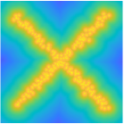
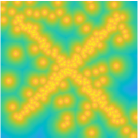
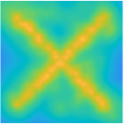
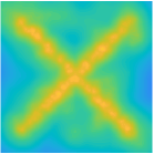
We consider two test images, one containing a solid letter A, and the other containing a letter X constructed as a sparse point-cloud in the regular grid, both corrupted by random noise-points added with probability . We compute both the MC-SDT and DET-SDT using . Different computed DTs, in noise-free and noisy conditions, are presented in Fig. 1 for qualitative assessment. The evaluation metric used is Average Absolute Distance Error (AADE) in the computed distance map, over all pixels, averaged over 100 repetitions with different noise realizations.
Results:
 |
 |
 |
 |
|
| (a) Noise-free DT | (b) DT | (c) MC-SDT | (d) DET-SDT | |
 |
 |
 |
 |
|
| (e) Noise-free DT | (f) DT | (g) MC-SDT | (h) DET-SDT |
Quantitative results are presented in Tab. 2. The stochastic methods exhibit substantially higher, and more consistent (in terms of std. dev.), accuracy than the standard DT in the presence of noise.
| DT | MC-SDT | DET-SDT | |
|---|---|---|---|
| Image A | 5.41 0.55 | 2.39 0.29 | 2.42 0.27 |
| Image X | 14.31 0.87 | 8.02 0.75 | 8.02 0.74 |
4.2 Template Matching
Template matching of (binary) images is a process of locating a particular region/object in the image by finding a location where a given template ”fits best”, i.e., where a distance between the template and the image is minimal (or where a similarity measure is maximal). In the search, we consider all possible translations of the observed template by vectors with integer coordinates, such that the template is completely included in the image. We minimize the bidirectional (asymmetric, being suitable for template matching) distance [12] based on Sum of Minimal Distances (SMD) [7], defined as
| (8) |
where and denote the complement sets of and , respectively. This distance measure has been shown to have a number of appealing properties, such as a smooth distance field subject to translation, rotation and affine transformations. One drawback that has been observed is that this distance is quite noise-sensitive in the sense that a few spurious points can create shallow local minima in its distance landscape. As a consequence, both local search (where the search stops upon finding a local minimum) or global search may result in many false detections and must be pruned in post-processing. This part of the study aims to investigate if noise-sensitivity of template matching with can be reduced if SDT is used in computation of instead of the (ordinary) DT.
Experimental Setup:
We consider the well-known Cameraman (grey-scale) image. We corrupt it with additive Gaussian noise (), Fig. LABEL:fig:tmresults1(a) and then threshold at intensity into a binary image, Fig. LABEL:fig:tmresults1(b). A binary template is extracted from the noise-free original, by thresholding at the same intensity level, Fig. LABEL:fig:tmresults1(c). Within the evaluation framework we compute the distance between the template and the image , for every position in the image where the template is completely included in the image. In this computation, we use , with , as the underlying DT for . The position where global minimum of is reached is recorded to evaluate if the correct location is recovered. The number of minima (NoM) is also computed for the distance field, as well as the catchment basin (CB) of the global minimum. The CB is the set of all image points which would, if used as initialization for a local search (using 8-neighbourhood steps), provide convergence to the global minimum. The evaluation metrics are averaged over noise realizations for each considered . Since the uncertainty factor corresponds to the standard DT, this evaluation includes comparison of performance of using standard DT and with using the here proposed SDT.
Results:
The results are presented in Fig. LABEL:fig:tmresults1(d-g). Figures LABEL:fig:tmresults1(d,e) show colored labelling (on a single realization) of the NoM and their corresponding CB, for standard DT, and for DET-SDT. Significantly decreased NoM, and visibly larger CB corresponding to the correct template position (red cross) characterize DET-SDT. The plots LABEL:fig:tmresults1(f,g) show the NoM and the size of a CB of the global minimum (in a percentage of the number of pixels in the image), as a function of the uncertainty factor . The results clearly show that the evaluation metrics improve in a stable and gradual way with increasing . The NoM exhibits a linearly decreasing trend, where the CB size initially exhibits a linearly increasing trend until , where a super-linear increase is observed. The know global minimum (correct match) is successfully recovered in all tests.
4.3 Watershed Segmentation
The watershed transform [4] is a transformation which partitions a grey-scale image into regions associated with the local minima of the image (or a number of defined seed points). Intuitively, the graph of the grey-level image is flooded with water coming out from the seed points (minima) and filling the corresponding basins. Where the basins of different seed points meet, ridge-lines mark a delineation of the different objects. One common approach for shape based watershed segmentation is to use the negative of the DT as the grey-scale image, and its minima (maxima in the original DT) as seed-points.
It is important to note that the watershed segmentation approach used here utilizes stochasticity in a very different way than the stochastic watershed segmentation [1] method, which randomly places seed points and yields a PDF of the ridge-lines which separate the objects in the image. The method presented here employs stochasticity to remove spurious optima, with the aim of achieving robustness to noise and preventing oversegmentation.
4.3.1 Separation of a Pair of Discretized Disks
Experimental Setup:
To evaluate the proposed method in a scenario with no additive noise, but merely digitization artifacts/noise, a synthetic benchmark was constructed: two equisized disks are positioned with random sub-pixel placements, so that they have some overlap, and then digitized (by Gauss centre point digitisation) on a regular grid into a binary image. Watershed segmentation is applied on the negated internal DT to separate the created object into two components. Figure LABEL:fig:wsresults1(a) shows the created binary object, where (b) an (c) present examples of segmentation (separation of the two disks). The radii of the disks are chosen to be pixels, to create reasonably sized objects with irrational radii. Following digitization, watershed segmentation is applied to the distance map resulting from the DT, MC-SDT and DET-SDT on the binary image. The resulting segmentations are analyzed w.r.t. the number of segmented objects, observing 200 repetitions of the experiment for every value of the distance between the centres of the disk within the range , with a step-size of . Considering that the disks can, in the continuous case, always be segmented into two components, we assume that 2 is the correct number of objects to result from the performed watershed segmentation. An uncertainty factor is selected based on tuning on a smaller set of repetitions and steps.
Results:
Figure LABEL:fig:wsresults1 shows the results of the disks segmentation (separation) experiment. Each plot shows the performance of the segmentation in terms of the fraction of the trials at which the various object counts occur, as a function of distance between the disk centres. We observe that the SDT-based methods perform similarly, and substantially better than the standard DT. Table 3 shows the Area Under the Curve (AUC) of the detection frequency corresponding to 2 segments.
| Method | DT | MC-SDT | DET-SDT |
|---|---|---|---|
| AUC: (2 segments) | 0.563 | 0.661 |
4.3.2 Watershed segmentation, a realistic example
Experimental Setup:
To evaluate the performance of the watershed segmentation when used with the proposed SDT method in a realistic setting, we observe the well known image Pears.png, to which we apply additive Gaussian noise with , Fig. LABEL:fig:wsresults2(a). We binarize the image (by thresholding), Fig. LABEL:fig:wsresults2(b), and segment it using watershed method with both DT and SDT.
Parameter values are: , , binarization threshold set to (manually selected on the noise-less image).
Results:
The segmentation results are evaluated subjectively. We find that the segmentations shown in Fig. LABEL:fig:wsresults2(d,e), which rely on SDT, clearly indicate advantage of the here presented approach, compared to classic DT which leads to heavy oversegmentation, caused by high sensitivity to noise.
5 Conclusion
In this study we have proposed a novel type of distance transform, the Stochastic Distance Transform. SDT is based on probability distributions of distances to image objects represented as Discrete Random Sets. The main advantage of the SDT over the classic DT is its adjustable robustness to noise, allowing to choose parameters controlling a level of sensitivity according to the application at hand. The proposed method’s utility and favorable properties are observed both through various synthetic tests and an illustrative natural example.
Future work includes an extended study of the theoretical properties of the proposed method, investigating (possibly adaptive) methods for reducing the biases of the resulting distance values, extending the empirical evaluation, and exploring further potential applications.
Acknowledgements
This work is supported by VINNOVA, MedTech4Health grants 2016-02329 and 2017-02447 and the Ministry of Education, Science, and Techn. Development of the Republic of Serbia (proj. ON174008 and III44006).
References
- [1] Angulo, J., Jeulin, D.: Stochastic watershed segmentation. In: PROC. of the 8th International Symposium on Mathematical Morphology. pp. 265–276 (2007)
- [2] Baddeley, A., Molchanov, I.: Averaging of random sets based on their distance functions. Journal of Mathematical Imaging and Vision 8(1), 79–92 (1998)
- [3] Bentley, J.L.: Multidimensional binary search trees used for associative searching. Communications of the ACM 18(9), 509–517 (1975)
- [4] Beucher, S.: Use of watersheds in contour detection. In: Proceedings of the International Workshop on Image Processing. CCETT (1979)
- [5] Borgefors, G.: Distance transformations in digital images. Computer vision, graphics, and image processing 34(3), 344–371 (1986)
- [6] Cuisenaire, O., Macq, B.: Fast k-NN classification with an optimal k-distance transformation algorithm. In: Signal Processing Conference, 2000 10th European. pp. 1–4. IEEE (2000)
- [7] Eiter, T., Mannila, H.: Distance measures for point sets and their computation. Acta Informatica 34(2), 109–133 (1997)
- [8] Goutsias, J.: Morphological analysis of discrete random shapes. Journal of Mathematical Imaging and Vision 2(2-3), 193–215 (1992)
- [9] Gustavson, S., Strand, R.: Anti-aliased Euclidean distance transform. Pattern Recognition Letters 32(2), 252–257 (2011)
- [10] Levi, G., Montanari, U.: A grey-weighted skeleton. Information and Control 17(1), 62 – 91 (1970)
- [11] Lewis, T., Owens, R., Baddeley, A.: Averaging feature maps. Pattern Recognition 32(9), 1615–1630 (1999)
- [12] Lindblad, J., Curic, V., Sladoje, N.: On set distances and their application to image registration. In: Image and Signal Processing and Analysis, 2009. ISPA 2009. Proceedings of 6th International Symposium on. pp. 449–454. IEEE (2009)
- [13] Lindblad, J., Sladoje, N.: Exact linear time euclidean distance transforms of grid line sampled shapes. In: International Symposium on Mathematical Morphology and Its Applications to Signal and Image Processing. pp. 645–656. Springer (2015)
- [14] Matheron, G.: Random sets and integral geometry. Wiley, New York; (1975)
- [15] Maurer, C.R., Qi, R., Raghavan, V.: A linear time algorithm for computing exact Euclidean distance transforms of binary images in arbitrary dimensions. IEEE Transactions on Pattern Analysis and Machine Intelligence 25(2), 265–270 (2003)
- [16] Moreno, R., Koppal, S., De Muinck, E.: Robust estimation of distance between sets of points. Pattern Recognition Letters 34(16), 2192–2198 (2013)
- [17] Rosenfeld, A., Pfaltz, J.L.: Sequential operations in digital picture processing. Journal of the ACM (JACM) 13(4), 471–494 (1966)
- [18] Saha, P.K., Borgefors, G., di Baja, G.S.: A survey on skeletonization algorithms and their applications. Pattern Recognition Letters 76, 3–12 (2016)
- [19] Saha, P.K., Wehrli, F.W., Gomberg, B.R.: Fuzzy distance transform: theory, algorithms, and applications. Computer Vision and Image Understanding 86(3), 171–190 (2002)