Abstract
This paper proposes a novel algorithm for image phase retrieval, i.e., for recovering complex-valued images from the amplitudes of noisy linear combinations (often the Fourier transform) of the sought complex images. The algorithm is developed using the alternating projection framework and is aimed to obtain high performance for heavily noisy (Poissonian or Gaussian) observations. The estimation of the target images is reformulated as a sparse regression, often termed sparse coding, in the complex domain. This is accomplished by learning a complex domain dictionary from the data it represents via matrix factorization with sparsity constraints on the code (i.e., the regression coefficients). Our algorithm, termed dictionary learning phase retrieval (DLPR), jointly learns the referred to dictionary and reconstructs the unknown target image. The effectiveness of DLPR is illustrated through experiments conducted on complex images, simulated and real, where it shows noticeable advantages over the state-of-the-art competitors.
keywords:
Complex domain imaging, phase retrieval, photon-limited imaging, complex domain sparsity, dictionary learning.xx \issuenum1 \articlenumber5 \historyReceived: date; Accepted: date; Published: date \Title Dictionary Learning Phase Retrieval from Noisy Diffraction Patterns \AuthorJoshin P. Krishnan 1,∗, José M. Bioucas-Dias 1 and Vladimir Katkovnik 2 \AuthorNamesFirstname Lastname, Firstname Lastname and Firstname Lastname \corresCorrespondence: joshin.krishnan@lx.it.pt (J.P.K)
1 Introduction
1.1 The Phase Retrieval Problem
Phase Retrieval (PR) is an important and challenging problem in many fields of science and technology. PR is a crucial step in most diffraction- or scattering-based physical measurement systems. In such systems, the signals being used, namely a non-coherent photon flux, laser, X-ray, or any other variants of the electromagnetic radiation, are diffracted through an object under examination. These diffracted signals encode the structural information of the object such as thickness, density, or refractive index, and are detected using a suitable sensor. Since the detectors sense the diffracted signals by converting the photon flux to electrons, the information related to phase of the signal is not recorded. This is a major limitation as important structural informations of the object are often coded mainly in the phase. PR aims at estimating the hidden phase from the intensity measurements. This is a challenging problem as there is no one-to-one relation between the phase and the measured intensity, which is proportional to the magnitude square of the field.
This paper discusses the phase retrieval problem in an optical imaging scenario. We would like, however, to remark that, in spite of being developed in a specific scenario, the proposed concept and algorithm is easily adapted to other imaging fields characterized by similar mathematical observation models.
Hereafter, we consider that the power spectral density, i.e., the magnitude squared of the Fourier transform, is the measurement provided by the sensor. This assumption is very reasonable and common in literature (Candes et al., 2013; Katkovnik, 2017; Candès et al., 2015). It is based on the fact that the optical wavefront at the sensor plane in the far field (i.e., at a large enough distance from the imaging plane) is well approximated by the power spectral density of the wavefront at the object plane. This result can easily be derived from the Fraunhofer diffraction equation for coherent imaging systems (Saleh and Teich, 2007; Goodman, 2005).
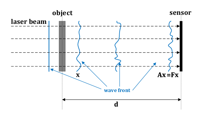
Fig. 1, courtesy of Katkovnik (2017), schematizes a lensless optical imaging system. A planar wavefont produced by a laser beam 111Here, without loss of generality, we assume that the intensity of the laser beam is constant over the object. is transmitted through an object (whose image to be inferred) and propagates until it reaches the sensor. The 2D PR problem in the vectorized form is as follows:
| find | ||||||
| subject to | (1) | |||||
where is the complex-valued wavefront with pixels at the object plane and is an matrix modeling the wavefront propagation from the object to the sensor plane, which, in the far field, is well approximated by DFT matrix , i.e., , is the component-wise magnitude operator, and accounts for measurement (or model) noise. The presence of the term in (1) makes this problem nonconvex and thus challenging.
1.2 Phase Retrieval: Applications, algorithms & recent trends
Phase retrieval field has a rich history, perhaps the proposal of phase contrast imaging in 1930 by Frits Zernike (Nobel prize 1953) is one of its early stage milestones. Another revolutionary contribution was in 1952 by David Sayre in the field of crystallography Sayre (1952). Perhaps the most important field that is benefited from PR algorithms is X-ray crystallography Millane (1990), Harrison (1993). X-ray phase-contrast imaging (XPCI) is a powerful tool in structural investigations Bonse and Hart (1965); Petrakov (2003); Snigirev et al. (1995); Wilkins et al. (1996); Pfeiffer et al. (2006). As already mentioned before, most of the physical measurement systems record only the intensity of the detected signal and this makes PR an unavoidable process in various fields, namely microscopy Miao et al. (59:387-410, 2008), optics Walther (1963), speech and acoustics Rabiner and Juang (1993), Balan et al. (2006), astronomical imaging Dainty and Fienup (1987), array imaging Chai et al. (2011), interferometry Demanet and Jugnon (2017), computational biology Stefik (1978), diffraction imaging Bunk et al. (63(4), blind deconvolution Baykal (2004), quantum mechanics Corbett (2006), Reichenbach (1965), quantum information Heinosaari et al. (2013), blind channel estimation in wireless communications Ahmed et al. (2014) Ranieri et al. , X-ray tomography Dierolf et al. (2010), differential geometry Bianchi et al. (60 (2002) etc.
The early approaches to PR fall under two categories of methods: error-reduction and gradient-based. The phase-retrieval problem defined in (1) is often formulated as the following least squares problem or empirical risk () minimization problem:
| (2) |
Error-reduction algorithms are iterative and guarantee to reduce error () in each iteration. The most popular family of PR algorithm, the Gerchberg-Saxton (GS) Gerchberg and Saxton (1972) and its variants Guo et al. (2015), Yang et al. (1994), comes under this category. These are iterative algorithms based on alternating projections between the object plane and the diffraction (Fourier) plane. A basic GS algorithm has four simple steps: (1) Forward projection: Fourier transform of the object wavefront; (2) imposing Fourier magnitude constraints at the Fourier plane: replace the modulus of the forward propagated wavefront with the measured intensity to form an estimate of the Fourier transform; (3) backward projection: inverse Fourier transform operation; and (4) imposing spatial-domain constraints at the object plane: modifying the backward projected wavefront by imposing support constraints in accordance with the prior information of the object.
Fienup, in his famous Hybrid Input-Output (HIO) algorithm Fienup (1982), addressed the slow convergence of the GS algorithms by imposing additional spatial-domain corrections. Although both GS, HIO and their variant algorithms are widely used in optical imaging, they suffer from stagnation at local minima due to the non-convex nature of the Fourier magnitude constrains.
An alternative class of methods to address PR is based on gradient searches. In this class, in each iteration, the wavefronts are updated in such a way that the partial derivative of the gradient of an error metric, which one seeks to minimize (e.g., ), is equated to zero. This line of attack is discussed in Fienup (1982), where, although the convergence rate of a steepest descent-based Fienup (1982) algorithm is low, its conjugate gradient-based version Lane (1991) is much faster.
The recent Wirtingling Flow (WF) algorithm Candès et al. (2015) is an iterative complex domain gradient descent technique. Although the gradient operation is not well-defined for complex domain variables, WF adopts a surrogate derivative, termed the “Wirtinger derivative”, and is characterized by special features, such as spectral initialization, non-trivial step-size parameter, etc. The truncated version of the WF algorithm, termed truncated Wirtingling Flow (TWF) algorithm Chen and Candes (2015) improves the initialization and descent procedures in an adaptive fashion by a statistically motivated regularizing technique, which filters out the terms bearing too much influence on the initial estimate or search directions. A surprising claim stated in Chen and Candes (2015) is that solving the quadratic equations (1) is “nearly as easy as solving linear equations”, which is a significant leap in many fields.
An alternative phase retrieval strategy has been proposed recently by exploiting the semi-definite relaxations. The set of quadratic equations represented by (1) is rewritten as linear equations in a higher dimension space. The phaseLift Candes et al. (2013) and PhaseCut Waldspurger et al. (2015) are two important algorithms in this category. In PhaseLift, the “lifting” is done by the variable transformation ,222 is the Hermitian operator which provides a convenient linear constraint in terms of the matrix variable . The underlying rank minimization non-convex problem is relaxed to a convex one yielding a semidefinite program (SDP). Similarly, in PhaseCut, the complex variable is separated into an amplitude component and a phase component, and only the phase component is ‘lifted’ and then optimized via SDP. But the matrix lifting in SDP-based approaches results a higher-dimensional variable, which, in turn, makes the algorithm computationally demanding compared to the alternating projection approaches.
A computationally light PR algorithm based on convex relaxation that operates in the natural domain of the signal is proposed in Bahmani and Romberg (2017). In this work, a “complex polytope” of feasible solutions is considered by relaxing the quadratic equations of phaseless measurements to inequalities. The desired solution would be one of the extreme points of this polytope which is found using a convex program.
In the recent decades, PR has been highly benefited from the advances in the field of compressed sensing and new imaging technologies. In line with the overview Kishore et al. (2015), we wish to mention two important approaches in phase retrieval which have been sprouted as a results of these advancements. They are (1) Phase front modulation based approaches and (2) Sparsity based approaches.
1.2.1 Phase front modulation
Phase front modifications Nugent et al. (2003), Johnson et al. (2008) are imaging techniques in which a known phase modulation is intentionally introduced into the object field. These phase modification are done through phase masks mounted on the wavefront propagation path and different masks lead to different diffraction patterns. An analogy from microscopy would be focusing one part of the sample to be examined and then repositioning the sample to exploit the spatial diversity. By shifting the phase mask or, equivalently, by using different masks, independent diffraction patterns, termed coded diffraction patterns (CDPs)Candes et al. (2015), are generated from the same illumination area of the object. The CDP introduces over-determination in the amplitude attenuation and phase shift of the wave diffracted through the object. Also, in a CDP, the recoded intensity at a sensor point have contributions from all points in the object. Spreading the information of one object point to all pixels of the sensor minimizes the the sensor noise and also mitigates the stagnation in the retrieval process Zhang et al. (2007).
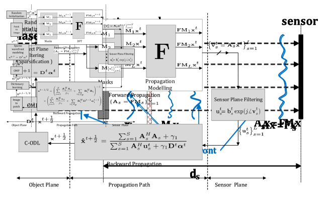
The setup shown in Fig. 2 corresponds to a modifications of that of Fig. 1, where a phase mask is incorporated. The corresponding PR problem is
| find | |||||
| subject to | (3) |
where are the wavefront propagation matrices given by . In our model, denotes the DFT matrix and is a phase mask which is a diagonal matrix of complex exponents, i.e., , where , are random phase values.
1.2.2 Sparsity meets Phase Retrieval
The concept of sparsity has received tremendous attention from various signal processing areas. Signals and images of the real world admit sparse representations when represented on suitable frames Elad (2010), which can be exploited to build low dimensional models. As in many areas, sparsity has become a hot topic in PR methods and algorithms. TSPR Jaganathan et al. (2017) and GESPAR Shechtman et al. (2014) are two important state-of-the-art algorithm that exploit sparsity. TSPR is a two-stage algorithms in which the support of the signal is estimated in the first stage and the signal is estimated in the second stage using a sparsity constrained PhaseLift framework along with the learned support. GESPAR uses an optimization-based greedy algorithm in which PR is reformulated as a sparsity-constrained least square problem.
Another important research line in the context of sparsity exploits the self-similarity Dabov et al. (2006); Afonso et al. (2015); Elad and Aharon (2006) exhibited by the natural images, which has been extensively exploited via patch-based approaches in various fields of image processing Dabov et al. (2007); Li et al. (2014); Deledalle et al. (2011). Since the phase images are natural images, they often exhibit high level of self-similarity. A number of phase imaging algorithms exploiting self-similarity has been recently introduced, namely the complex dictionary-based SpInPhase Hongxing et al. (2015), the complex domain Mixture of Gaussian -based MoGInPhase Joshin and Bioucas-Dias (2017), the BM3D-based CBM3DKatkovnik and Egiazarian (2017), and the sparse approximation of the object phase and amplitude SPAR Katkovnik (2017).
SPAR Katkovnik (2017) is a recent PR algorithm that shows remarkable performance in highly noisy scenarios, compared to the state-of-the-art algorithms. SPAR is built on a classical GS framework with additional features of random phase modulation of the wavefront and sel-similarity regularization of the phase and amplitude. The two stages of filtering, i.e., filtering the noisy (Poissonian) observations at the sensor plane and filtering the phase and the amplitude at the object plane, make this algorithm a step forward in noisy PR. SPAR exploits the self-similarity of complex domain patches by separately applying sparsity to the phase and amplitude components. Since the phase is restored modulo, the recovering of the absolute phase is carried out by including a phase unwrapping Bioucas-Dias and Valadao (2007) step. This is a sensitive part of SPAR, as the phase unwrapping is known to be an NP-hard problem. Another downside of SPAR is its high computational complexity, compared with that of GS.
1.3 Proposed algorithm and Contribution
Inspired by SPAR Katkovnik (2017) and by SpInPhase Hongxing et al. (2015), we propose a new algorithm, termed Dictionary Learning Phase Retrieval (DLPR), for PR from noisy diffraction pattern. DLPR is derived under a variational framework and is developed for both Poissonian and Gaussian observation models. We adopt the classic alternating projection-based framework (GS Gerchberg and Saxton (1972)), and incorporate 1) the wavefront modification detailed in Section 1.2.1, 2) filtering at the sensor plane for Poissonian (or Gaussian) observation, and 3) filtering at the object plane using dictionary-based sparse coding in the complex domain. We remark that, recently, a dictionary based PR algorithm is proposed in Tillmann et al. (2016), which makes use of a real valued dictionary and deals with real valued object, whereas DLPR deals with complex valued dictionary and object, which is an essential requirement in a practical PR scenario that often involves complex valued wavefronts. One of the remarkable advantages of sparse modeling in the complex domain is that it gets rid of the ambiguity due to phase wrapping, which makes it very robust to the heavily noisy observations, compared to the SPAR algorithm. The main contributions of the proposed work is summarized below:
-
1.
A variational reformulation of the PR problem that incorporates a dictionary based sparse regression in the complex domain.
-
2.
An algorithm that jointly retrieves phase and learns the dictionary yielding sparse representations (codes) for the complex domain patches of the object wavefront.
-
3.
An extension of the algorithm to a class-specific scenario, where the dictionary is learned from clean images of the same class.
The paper is organized as follows: in Section 2, the sparsity modeling for the complex domain wavefront is discussed. This section also introduces Poissonian and Gaussian observation models. The DLPR algorithm is derived in Section 3, by solving a step-by-step variational formulation for the forward propagation, the sensor plane filters for Poissonian and Gaussian observations, the backward propagation, and the sparse modeling at the object plane. In Section 4, an experimental study and characterization of the algorithm performance are provided including comparisons with relevant state-of-the-art algorithms.
2 Problem formulation
2.1 Sparse regression-based wavefront modeling
Let the vectorized complex domain image wavefront be represented as
| (4) |
where is the positive amplitude, is the absolute phase of the object wavefront and the operation stands for the element-wise (Hadamard) multiplication. Herein, all functions applied to vectors are to be understood as component-wise. One important factor to be noted here is that the accessible phase of a complex wavefront, which is extracted from the -periodic complex sinusoidal function, undergoes phase wrapping as defined below:
| (5) |
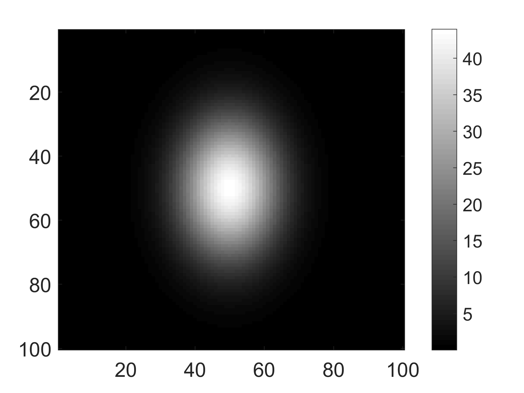
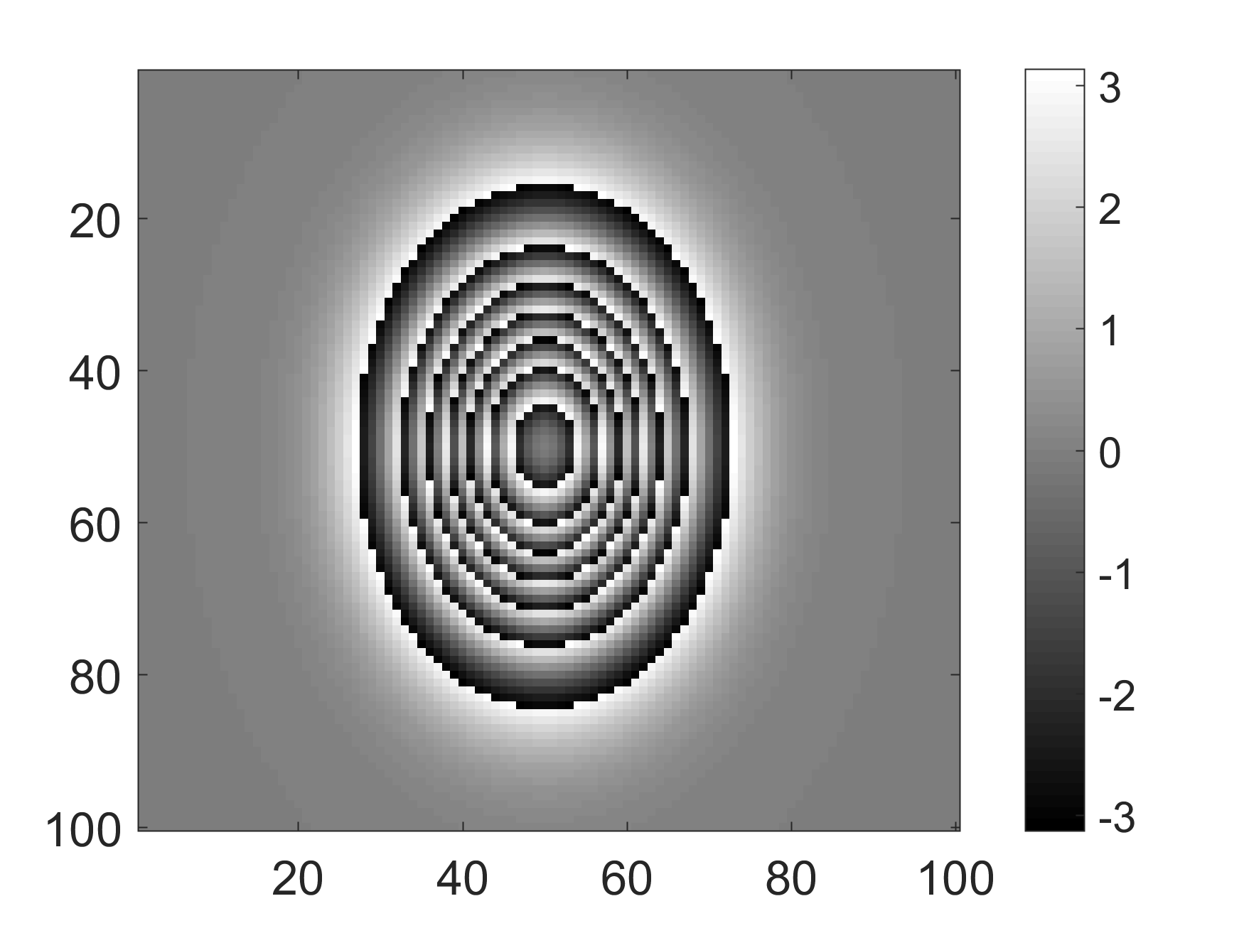
where is the wrapping operator that performs the 2-modulo phase wrapping operation. In the ensuing text, we use the notation , and term as the interferometric phase. We remark that the interferometric phase may be directly obtained from the image as . The interferometric phase is a non-linear function of the absolute phase and possess a pattern like discontinuities, called interferometric fringe patterns, as illustrated in Fig. 3.
Regarding the sparse modeling of a set of images , one can consider their amplitude and phase independently. However, from , or any estimate of it, we have only access to the corresponding interferometric phase, which raises a number of issues on how to model that phase, since the sparse models are usually specified in terms of the absolute phase. A solution to address this issue is to perform phase unwrapping using a suitable algorithm (e.g., PUMA Bioucas-Dias and Valadao (2007)), obtaining estimates of the absolute phase and then performing sparse modeling on it, as done in Katkovnik (2017). But the unwrapping algorithms are highly sensitive to noise and image discontinuities larger than . Also, in many practical applications, the phase and amplitude are strongly correlated and a decoupled sparsification of them is equivalent to assume that they are statistically independent, thus failing to exploit the correlation that might exit between them.
Here, we adopt the viewpoint introduced in Hongxing et al. (2015) to introduce a new PR strategy in which sparse modeling of the wavefront is done in the complex domain. This new strategy has the following distinct advantages: 1) inherent exploitation of the phase-amplitude correlation, as they are treated together in the complex domain form of wavefront, and 2) increased robustness to the noise, as the phase unwrapping is not used.
Sparse and redundant representations are recent and active research topics in signal and image processing Elad (2010) and have wide applications in many areas, such as denoising, restoration, interpolation, compression, sampling, recognition etc., to list only a few. The patch-based approaches are very popular in this context. Motivated by the recent phase imaging techniques Hongxing et al. (2015), Joshin and Bioucas-Dias (2017), Katkovnik et al. (2014), Katkovnik and Egiazarian (2017), we stress that, if and are self-similar, then their complex version should also be self-similar (see Hongxing et al. (2015) for further details). This means that it is possible to find similar complex domain patches located at different parts of the wavefront, which opens the door to sparse representations, where each complex image patch is represented by a linear combination of a small number of vectors, often termed atoms, from a (possibly learned) dictionary. Herein, we adopt this perspective to the optical imaging scenario of interest. The assumption of self-similarity results naturally from the fact that the involved amplitude and phase images are from real world objects.
As a natural follow up of the above discussion, we put forward a new idea for an optical wavefront modeling based on sparse regression using complex domain dictionaries. We follow a patch-based approach for the sparse wavefront modeling. Let and denote, respectively, a matrix that extracts the square patch of size from the wavefront image and the extracted patch of size . It is to be noted that the superscript in indicates that is a patch and the same notation is used hereafter. We also, remark that the rows of are a subset of the rows of the identity matrix of size . The index of a given patch refers to the wavefront image pixel corresponding to the top left hand side of the patch. Using these definitions, the patch aggregation, i.e., patches to image transformation can be realized using the following equation:
| (6) |
where is the Hermitian operator and is the sum of all patches put back into their original locations. We emphasis that the matrix is diagonal and its diagonal element indicates the number of times the pixel appears in the set of extracted patches. The patches are extracted and later aggregated in an overlapping manner and we refer to Hongxing et al. (2015) for more details on the decomposition and composition of the patches.
To better understand the sparse regression, at this point, we assume that a dictionary for sparsely representing a complex patches , , is available. By sparse regression, we mean that any patch , , may be represented as a linear combination of few columns, often termed atoms, from . Regarding the patch , our sparse wavefront modeling is formally defined as follows:
| (7) |
where is the optimization code for , is a parameter controlling the reconstruction error, and denotes the pesudo-norm of , i.e., the number of nonzero elements of the vector . The constrained optimization (7) has the following interpretation: since we are minimizing the zero norm of the code, the optimization aims to find an with the fewest number of non zero entries, keeping the reconstruction error below a pre-controlled value . We incorporate the sparse regression (7) in the phase retrieval algorithm to model the object wavefront and this, in turn, serves as a filter at the object plane of the optical setup. The algorithms for learning dictionary and code will be discussed later in the Section 3.
2.2 Noisy observation modeling
The observation model adopted in many PR algorithms assumes a noiseless scenario. But in practice, the measured intensities at the sensors are often corrupted by noise. Two common sources of noise are 1) the random motion of the charge carrier such as thermal noise generated in the sensor, which is modeled by additive white Gaussian perturbations, and 2) photon-limited measurements, which are modeled by Poissonian perturbations. So, we develop the DLPR algorithm by considering either Poissonian or Gaussian noise observation models.
2.2.1 Poissonian observation model
The optical imaging systems usually capture the wavefront intensity as the counts of photons hitting a detector. There are many practical limitations that restrict us from using a high energy radiation with sufficient number of photons. For instance, in medical X-ray imaging, a high energy radiation can cause damage to the specimen, which is often a human organ. Also, an imaging system that can deploy only low exposure time or can use only limited amount of light (e.g., night vision and astronomical imaging systems) results in a low number of photons. Phase imaging using such low energy radiation is termed as photon-limited phase imaging, which results in heavily noisy registered measurements. The widely used additive Gaussian noise model fails to accurately model such discrete observations and, instead, a Poisson distribution shall be used Soulez et al. (2016), Raginsky et al. (2010), Salmon et al. (2014),Harmany et al. (2010).
In the presence of Poissonian noise, we assume that the components , for and , have Poisson distributions with parameters ; that is
| (8) |
where stands for Poisson distribution with parameter . Now let us consider a photon-limited imaging scenario and use the scaling factor to scale the mean value of the photon count. We restate (8) as
| (9) |
Here is an important parameter that controls the photon-count, which in turn controls the noise level. In a practical imaging system, is a function of various factors such as exposure time, sensor sensitivity, etc. Using the Poisson distribution formula, model (9) can be rewritten as
| (10) |
where is the photon count at the sensor. To understand the effect of on the noise level, we define signal-to-noise ratio (SNR) at the sensor as the ratio between the square of the mean and the variance (equal to mean for Poisson random variable) of , yielding
| (11) |
Expression (11) shows that SNR grows linearly with . Definition (11) motivates us to write a global estimate of SNR, as
| (12) |
2.2.2 Gaussian observation model
We also consider the widely used Gaussian noise that models, e.g., the thermal noise at the sensor. In this case, the observation model is
| (13) |
where , is a set of independent and identically distributed (i.i.d.) random variables, and stands for the standard deviation of the noise.
3 Dictionary Learning Phase Retrieval (DLPR) algorithm
We propose a novel idea, which we term as DLPR, to address the PR problem discussed in (3). DLPR is an alternating minimization algorithm that exploits the dictionary based sparse modeling of the object wavefront. The sparsification improves the conditioning of the inverse problem and its robustness to noise. The algorithm is derived for both Poissonian and Gaussian observation models and is developed based on the optical setup as discussed in Fig. 2.
3.1 DLPR for Poissonian Observation model
Referring to the Poissonian observation model (10), we state our PR problem as the estimation of from the noisy observations . The corresponding negative log-likelihood (after neglecting the constant terms) is
| (14) |
or equivalently
| (15) | ||||
A likelihood formulation similar to (15) is used in Candès et al. (2015) and Chen and Candes (2015) in which the focus is to maximize by computing using Wirtinger derivatives Adali et al. (2011) in an iterative manner. Here, however, we take a different approach by converting the hard constraint into a quadratic penalty and including a dictionary-based sparse regression term, which promotes image self-similarity. The DLPR variational formulation is as follows:
| (16) |
with
| (17) |
where is a convex set to be defined later, , and . The parameter controls the level of sparsity and control the weights of the quadratic penalties. Let us introduce the notation
| (18) | ||||
| (19) |
and use it to rewrite (3.1) as
| (20) |
The objective function in (20) is non-convex w.r.t. to the variables ). We address this issue by alternating minimization methods, which is a common approach to tackle this sort of non-convexity Rakotomamonjy (2013). As per this strategy, the likelihood is optimized by considering one variable at a time, treating the others as constants. Below we derive the optimization w.r.t. each variable. For each optimization, we rewrite the objective function by considering the terms depending on the optimization variable and disregarding the other terms.
Problem 1: Optimization w.r.t.
| (21) |
Given that (21) is decoupled w.r.t. , for and , we have , where is the proximity operator Combettes and Pesquet (2011) of the function computed in Soulez et al. (2016) and given by (see Katkovnik and Bioucas-Dias (2014) for further details)
| (22) | ||||
| where | ||||
| (23) | ||||
| For large values of the scale factor , we have | ||||
| (24) | ||||
Also from (10), it follows that a very high value of the scaling factor models the noiseless observations where the Poissonian model can be replaced with a deterministic model with probability 1. In this case we can write
| (25) | ||||
| Using (24) and (25), we rewrite (22) to obtain the amplitude update formula, for noiseless observation, as follows: | ||||
| (26) | ||||
Problem 2: Optimization w.r.t.
| (27) |
The minimum condition on (27) obtained by equating Wirtinger derivative for complex domain function to zero, i.e., , leads to the following least-square equation:
| (28) |
and to the solution:
| (29) |
We remark that i) the matrix is diagonal and the th diagonal element (say ) represents the number of times the pixel appears in the set of extracted patches, ii) For the propagation matrix (see description of (3)), , where is the identity matrix of order and iii) the vector is the sum of the reconstructed patches put back into their original locations. From the remarks i) and ii), it can be shown that the matrix to invert in (29) is diagonal with its diagonal entries given by . Thus the inversion of the large matrix can easily be precomputed.
Problem 3: Optimization w.r.t.
Given that the optimization w.r.t. is decoupled w.r.t. , for , the optimization w.r.t. amounts to compute
| (30) |
Optimization (30) is NP-hard due to the presence of norm Natarajan (1995). This issue is often circunvented by replacing the norm with a convex surrogate, often the norm, as seen in LASSO Tibshirani (1994), BPDN Chen et al. (1998), etc. However, and in line with the findings in Hongxing et al. (2015) and Mairal et al. (2009), we use a greedy algorithm, namely the orthogonal matching pursuit (OMP) Pati et al. (1993), to find an approximate solution of (30), which is computationally light and provides competitive results compared with those obtained by convex approximations to the norm.
The pseudo code for Complex domain OMP, courtesy of Hongxing et al. (2015), is shown in Algorithm 1.
In the above algorithm, is a matrix holding the atoms of indexed by and is the pseudo-inverse of . Also, represents the components of with indexes in .
Problem 4: Optimization w.r.t.
If the dictionary is known beforehand, the optimization w.r.t. is disregarded. However, if is unknown beforehand, we should solve the quadratically constrained quadratic program (QCQP)
| (31) | ||||
| s.t.: | (32) |
where the convex set is introduced to prevent the dictionary atoms being arbitrarily large, which in turn leads to arbitrarily small values of the codes . We remark that the presence of the terms in the objective function promotes sparse codes and, therefore, as desired, dictionaries are able to sparsely represent the restored patches. In a large number of experiments, we have observed, however, that the quality of the dictionary, regarding its ability to produce sparse codes, improves if we include an norm in the optimization (31) and solve simultaneously w.r.t. and , that is, if we solve,
| (33) | ||||
| s.t.: |
These findings are in line with those observed in Mairal et al. (2009) and Hongxing et al. (2015).
In (33), the joint optimization with respect to and is not convex, although it is convex with respect to each variable alone. This naturally invokes the alternating minimization methodology, in which one variable is minimized at a time keeping the other one fixed, in an iterative manner.
The real domain version of the optimization problem (33) was solved in Mairal et al. (2009) using the alternating minimization framework. More recently, its complex domain version was proposed for interferometric phase image estimation Hongxing et al. (2015) with slight modifications, which we term as C-ODL. Both ODL and C-ODL uses BPDN for sparse coding, i.e., the optimization w.r.t. , and projected block-coordinate descent method to update the columns of the dictionary. The BPDN problem in Mairal et al. (2009) is solved using Least Angle Regression (LARS) Efron et al. (2004), whereas in Hongxing et al. (2015) a much faster algorithm called sparse regression by variable splitting and augmented Lagrangian (SpaRSAL) is introduced for that purpose. We adopt the dictionary learning methodology proposed in C-ODL, whose pseudo code, courtesy of Hongxing et al. (2015), is shown in Algorithm 2.
3.2 DLPR for the Gaussian Observation model
We now derive DLPR for the Gaussian noise as detailed in (13). Then, the likelihood function in (3.1) can be rewritten as
| (34) |
Comparing (3.1) and (34), it is clear that DLPR optimization formulations are the same w.r.t. the variables , , and , which are derived in the Sections 3.1, 3.1 and 3.1 respectively. The only difference is in the amplitude update at the sensor plane, i.e., the optimization w.r.t . Minimization w.r.t. on (34) leads to the following Cardan equation, whose solution yields Soulez et al. (2016), Katkovnik and Astola (2012), Katkovnik (2017):
| (35) |
We remark here that, as the value of changes from to , the solution of (3.2) changes from to .
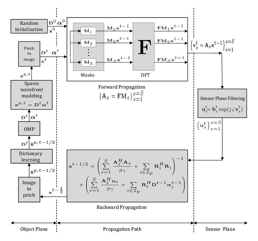
Pseudo code for the proposed DLPR algorithm, which combines the results derived in 3.1 and 3.2 for forward propagation, sensor plane filtering, backward propagation, and object plane sparsification is given in Algorithm 3. A schematic representation of the DLPR algorithm in the form of a block diagram is shown in Fig. 4. To better understand the signal flow of DLPR in relation with the optical setup 2, the block diagram is partitioned into 3 regions: i) Object plane - All the operations related to the wavefront sparse modeling, namely patch formation, dictionary learning, OMP, sparse regression and patch aggregation are part of this region. These blocks perform the operation given by the steps- 5, 6, 7, 8 & 9 of Algorithm 3. ii) Propagation path- This is the middle region of the schematic representation and models the forward and backward optical propagations described by step-2 and step-4 of Algorithm 3. ii) Sensor plane- The filtering operations at the sensor plane (step-3 of Algorithm 3) for Poissonian and Gaussian observations are included in this part.
4 Experiments and Results
In this section, we present a series of strong empirical evidences, using real and synthetic data, to illustrate the effectiveness of DLPR. Prior to the results, the details regarding the experimental setup are described below:
Optical setup: We restrict our optical setup to the lenseless imaging scenario, as illustrated in Fig. 2, which uses coded diffraction patterns for optical imaging. To implement the wavefront modulation, in alignment with the works presented in Candès et al. (2015), Chen and Candes (2015) and Katkovnik (2017), a random phase value sampled from the set is selected with equal probability for each pixel of the mask.
State-of-the-art competitors: The proposed DLPR algorithm is designed mainly for moderate and highly noisy scenarios. The recent TWF algorithm Chen and Candes (2015), designed for noiseless or small level noisy data, is chosen for comparison purposes. To the best of our knowledge, SPAR Katkovnik (2017) is the state-of-the-art for retrieving phase from the noisy observations and is a good candidate for the comparisons. We also consider a third candidate, which we term as GS-F algorithm, by skipping the sparse modeling of the wavefront at the object plane, i.e., by making the substitution , in Algorithm 3.The main rationale behind GS-F is that it helps to visualize how much improvement, in terms of performance, is contributed by the proposed sparse wavefront modeling. The performance of the conventional GS algorithm is expected to lag behind GS-F in noisy observation scenarios, as the GS lacks sensor plane filtering.
Although we consider SPAR, TWF, and GS-F for comparison purposes, the main competitor of DLPR is SPAR as it includes sparsity based object wavefront filtering aiming at good performance for noisy data. Since the SPAR algorithm applies sparsity on absolute phase, phase unwrapping has to be implemented to obtain the absolute phase in each iteration, which sets a bottleneck to the performance of SPAR, especially for highly noisy data. We make use of the publicly available MATLAB demo-codes444http://www.cs.tut.fi/sgn/imaging/sparse/ for SPAR and TWF.
DLPR parameter settings: Parameter settings are crucial in DLPR’s performance. The parameters of Algorithm 3 are heuristically set to the following values: for Poissonian observations and for Gaussian observations. For the wavefront modulation, SPAR Katkovnik (2017) suggests a value of . Without loss of generality, in alignment with the suggestions provided in Katkovnik (2017), all our experiments are conducted by keeping , i.e., for 12 observations with different phase modulation masks. The dictionary learning (C-ODL) 2 and OMP 1 sub-iterations are tuned to their best performance as per the parameter settings described in Hongxing et al. (2015). The patches used in all experiments are square, having dimension , extracted with unit stride.
We also remark that the algorithms chosen for comparison, i.e., SPAR, GS-F and TWF, are tuned to their optimal performances by using the parameter settings given in Katkovnik (2017).
Performance evaluation: Since the phase is the main focus of a typical PR problem, the performance of DLPR is evaluated based on the quality of the retrieved phase using Root Mean Square Error (RMSE) defined as
| (36) |
where is the wrapping operator defined is (5) and is the estimate of the true wrapped phase .
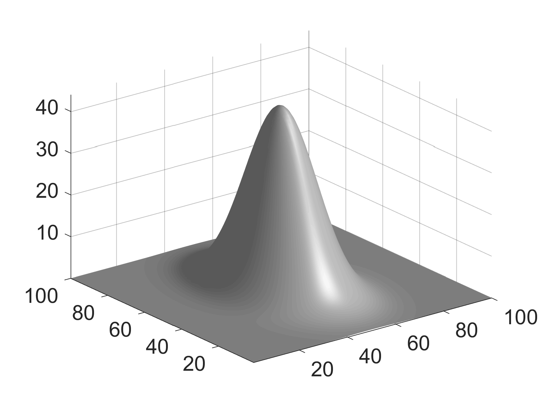
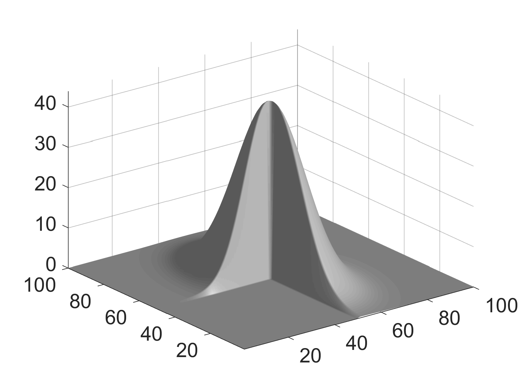
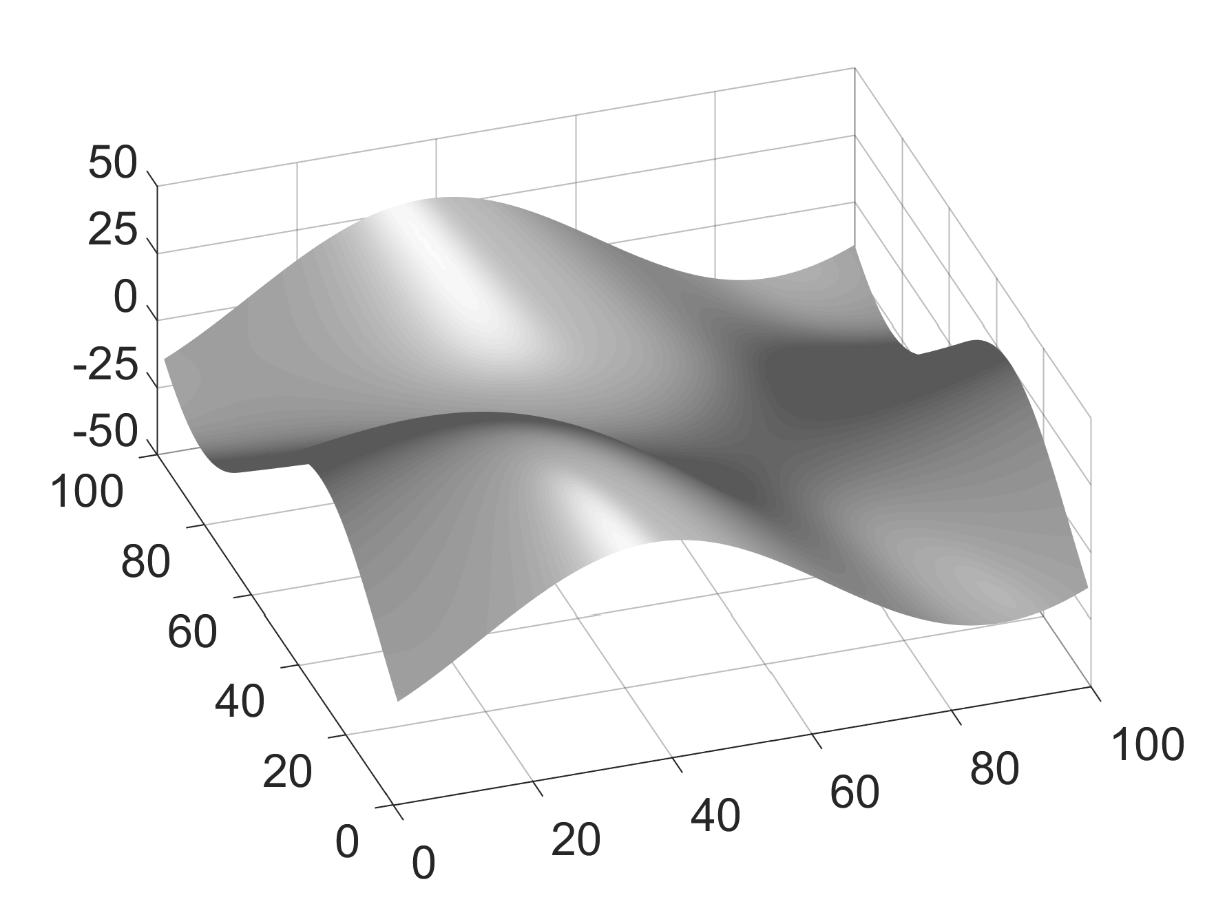
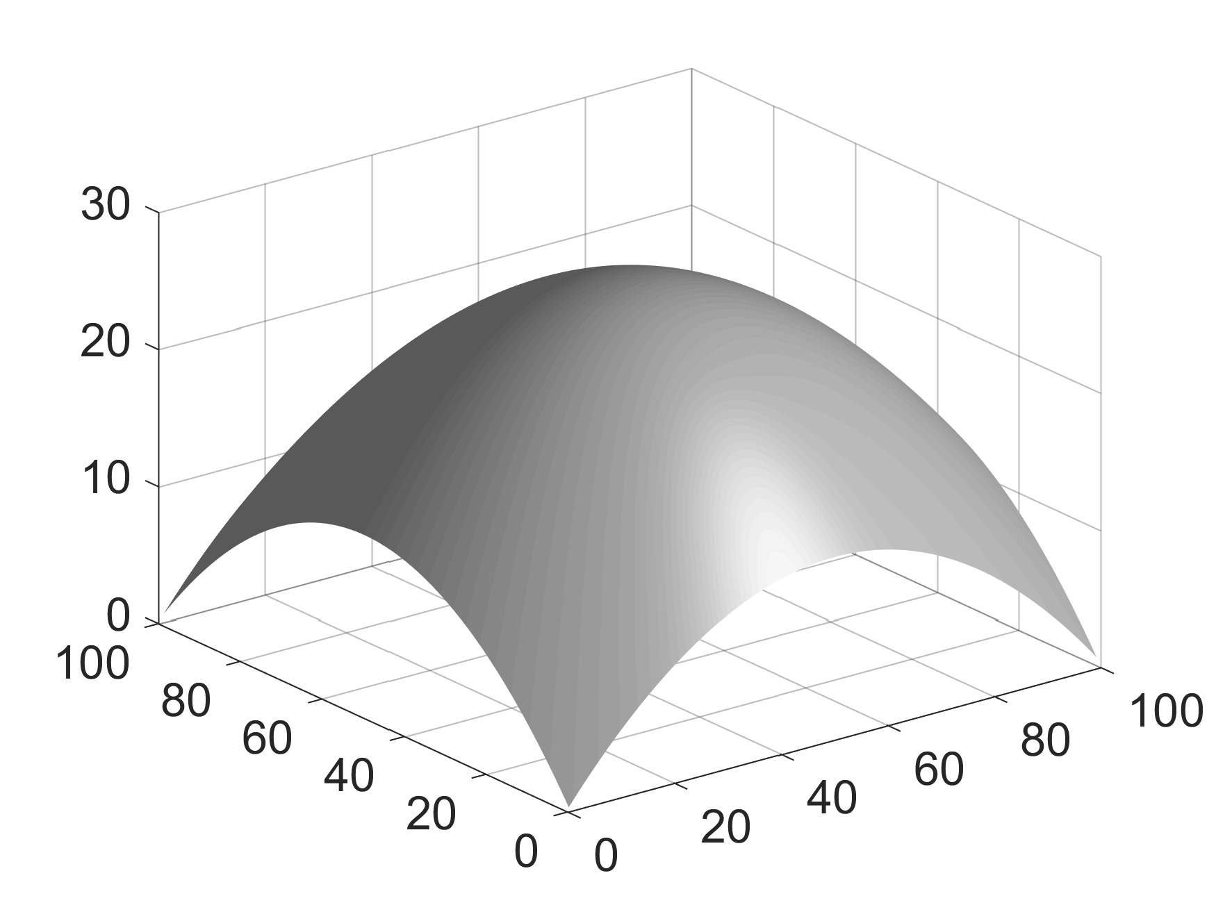
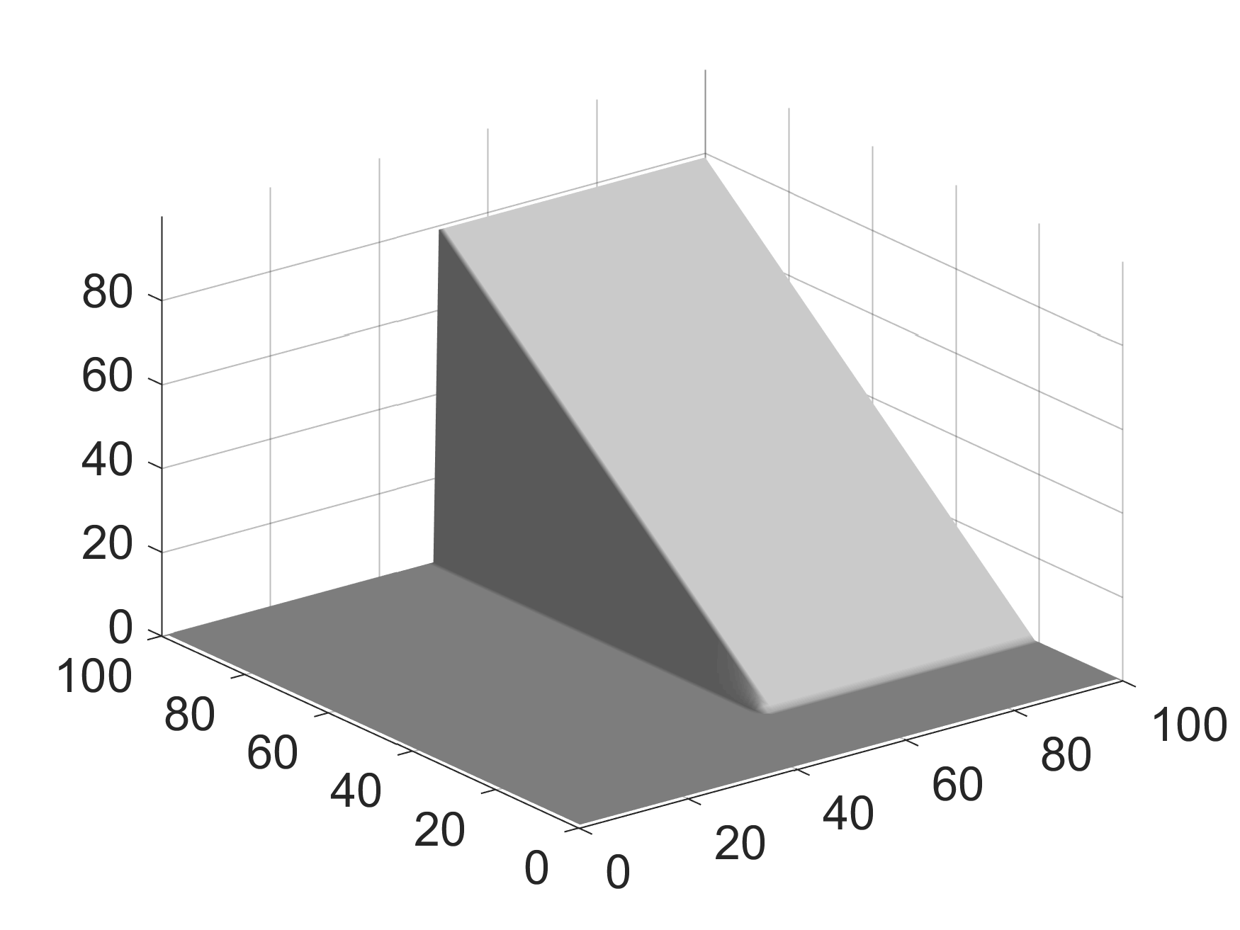
Synthetic data set: In an optical wavefront , the vectorised phase image and amplitude image can be quite correlated. In order to simulate various amplitude-phase relationships, we create different groups of complex signals in which the phases and amplitudes are related in different ways. We introduce the following formula to relate phase and amplitude in different ways:
| (37) |
where and are parameters used to control the level of amplitude and the function is used to control the correlation between phase and amplitude. Based on (37), we define the following groups of complex signals:
-
1.
Group-1: Invariant amplitude, i.e., .
-
2.
Group-2: Independent amplitude, i.e., amplitude and phase are two unrelated images.
-
3.
Group-3: Amplitude and phase are highly similar. .
-
4.
Group-4: Amplitude and phase are less similar. .
Using the above definitions for the image amplitudes and the simulated phase surfaces as shown in Fig. 5, nine different complex valued synthetic data are generated, which are summarised in Table 1.
| Sig No | amplitude | phase | Group |
| 1 | constant | Trun. Gaussian | 1 |
| 2 | constant | Shear Plane | |
| 3 | Mountain | Shear Plane | 2 |
| 4 | Quadratic | Trun. Gaussian | |
| 5 | Gaussian | Shear Plane | |
| 6 | Highly similar | Trun. Gaussian | 3 |
| 7 | Highly similar | Shear Plane | |
| 8 | Less similar | Trun. Gaussian | 4 |
| 9 | Less similar | Shear Plane |
4.1 Poissonian Observations
4.1.1 Experiments using synthetic data set
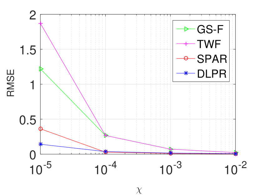
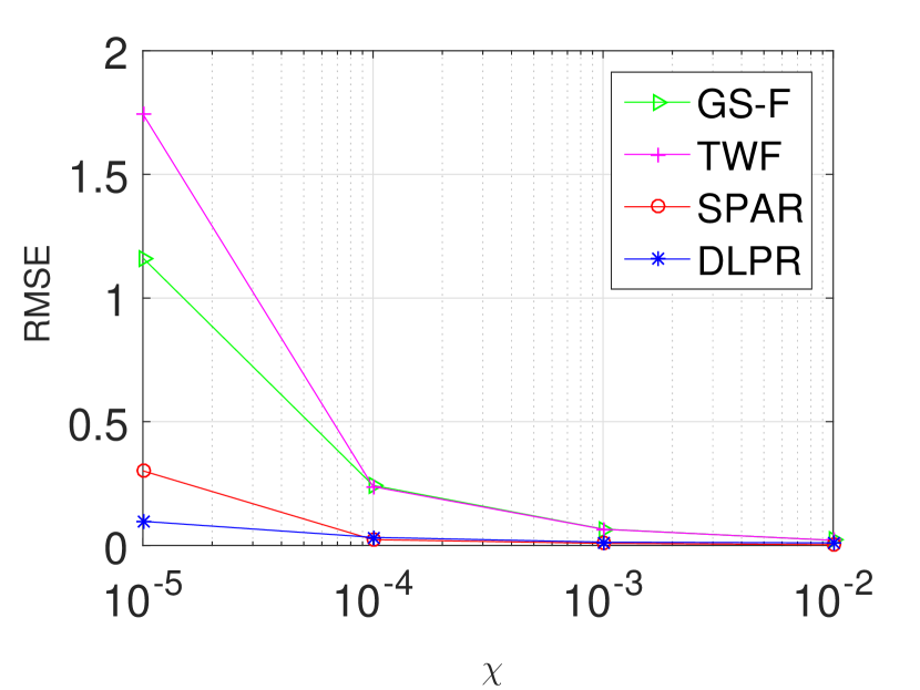
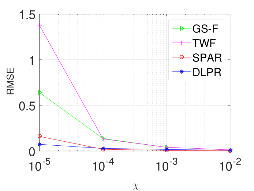
In this section, the experiments conducted using the data set given in Table 1 are presented. DLPR is tested for each group in the Table 1 by considering noise power ranging from high to medium level, i.e., . SNR values corresponding to these noise levels are respectively dB. RMSE values of the retrieved phase, averaged for each group, are given in Fig. 6. The performances of SPAR, TWF and GS-F are also included in the same figure. It is evident from the figure that the DLPR shows remarkable improvement over TWF and GS-F. In comparison with SPAR, DLPR performs better for heavy noisy data (). This observation is in clear alignment with our early intuition about DLPR. On the other hand, for medium level of noise, DLPR and SPAR give very close results. It should be noted that the low-noise scenario is not considered here as the objective of our algorithm is to retrieve phase from highly noisy observations. However, we remark that when the observation mechanism is noise free or with very low level of noise, all the four algorithms show similar performances.
4.1.2 Phase unwrapping
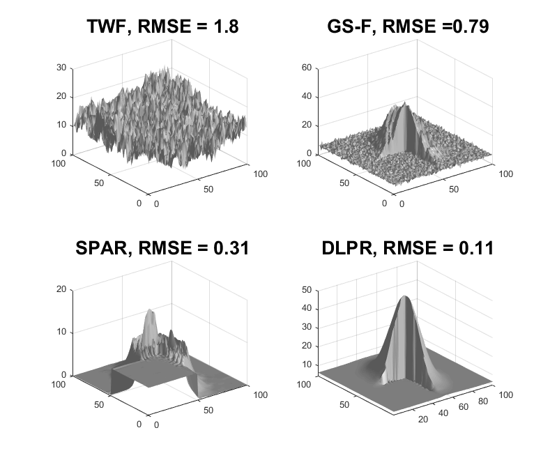
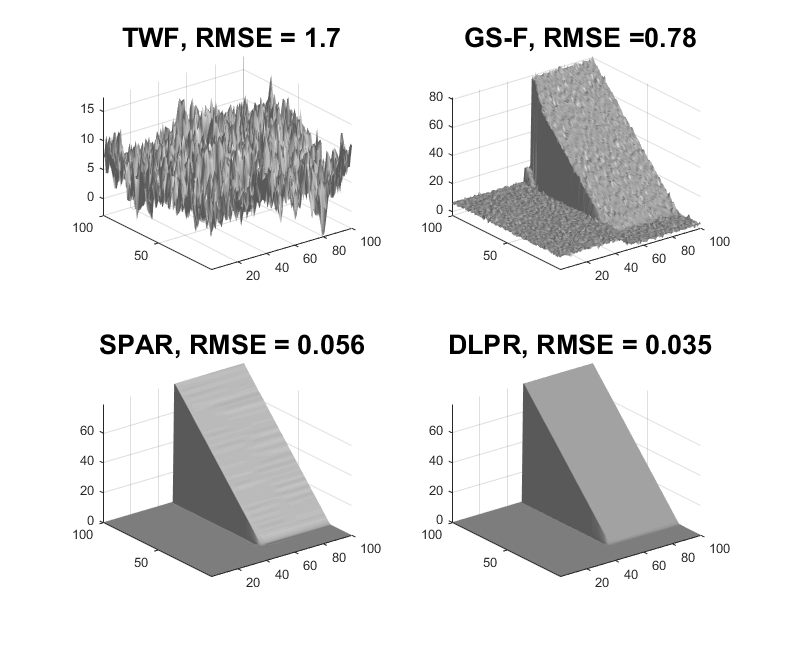
In a practical PR scenario, the phase obtained from retrieved complex wavefront is wrapped. The absolute phase is obtained by phase unwrapping in which the quality of the retrieved wrapped phase is a crucial factor. The following experiment is a qualitative illustration to show that the high quality of the phase images retrieved through DLPR underlies the good results during the unwrapping step. Here the phase retrieved from heavily noisy observations are unwrapped using PUMA algorithm Bioucas-Dias and Valadao (2007) (state-of-the-art in phase unwrapping). It is evident from Figs. 7(a) & 7(b) that TWF and GS-F provide very poor estimates. Compared to these two algorithms, DLPR and SPAR perform better. For shear plane 7(b), DLPR estimate is slightly better compared to SPAR. But for truncated Gaussian 7(a), DLPR is much better than SPAR.
4.1.3 Experiments using real MRI interferograms
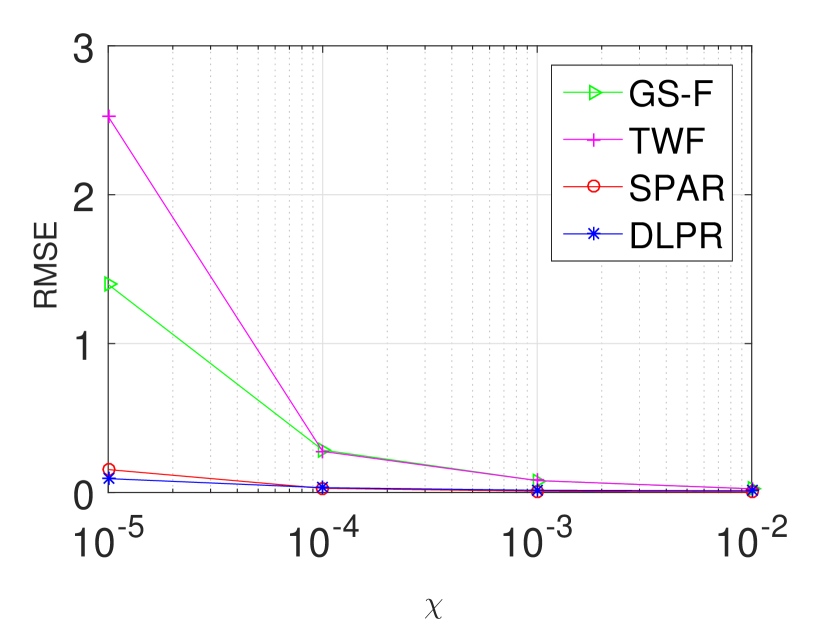
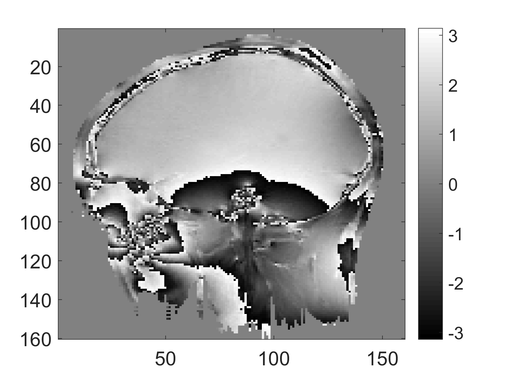
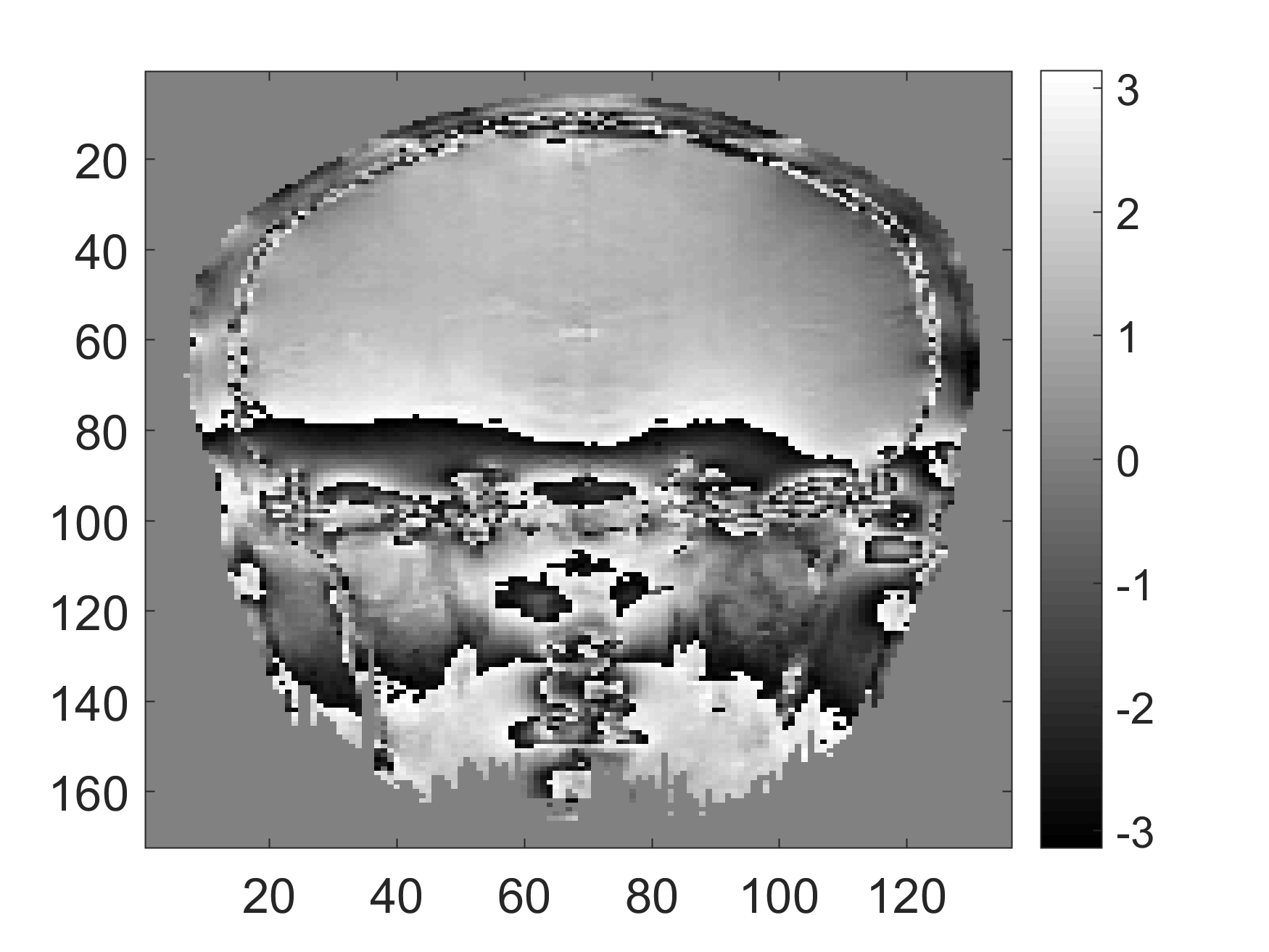
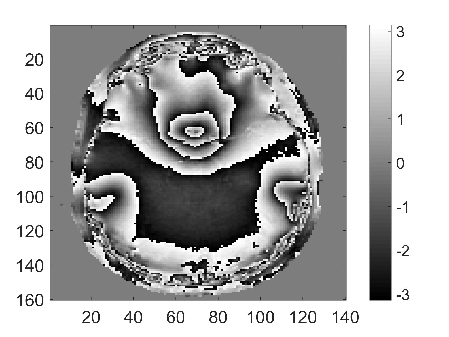
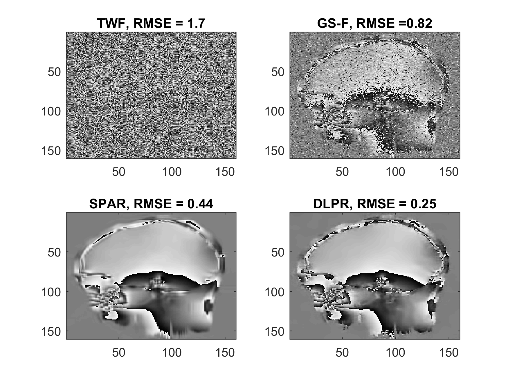
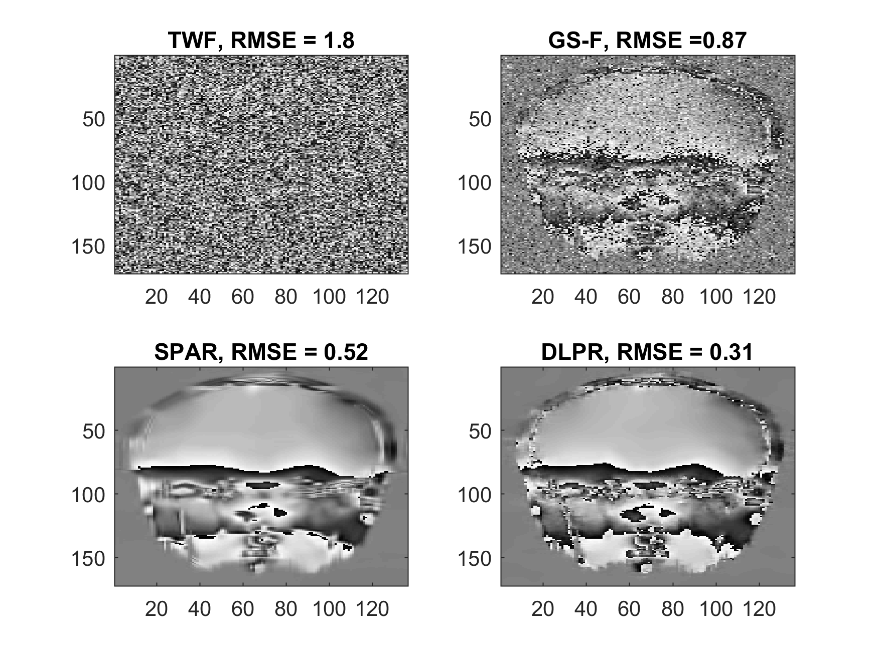
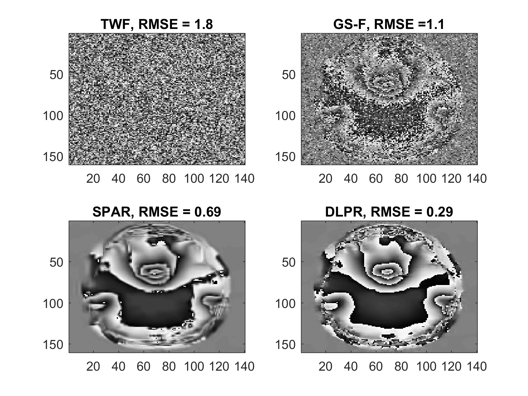
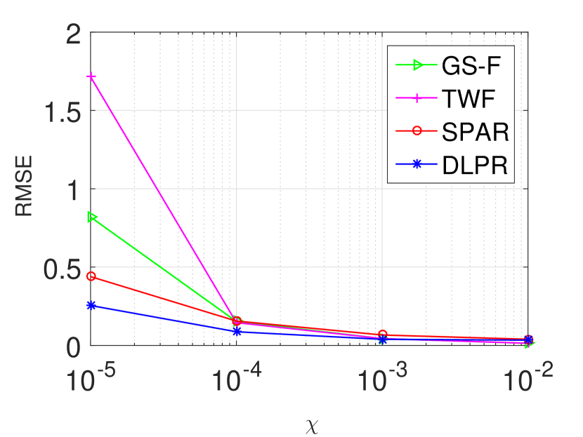
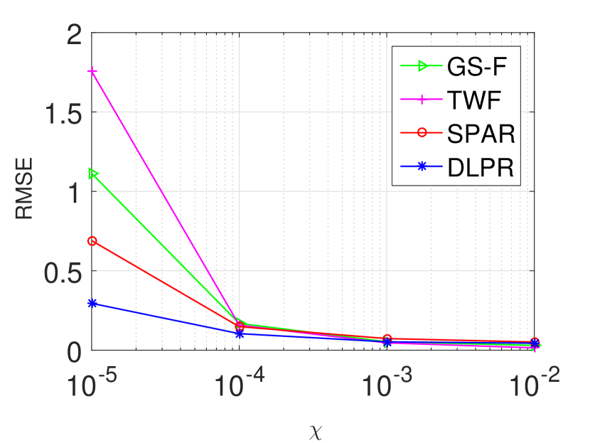
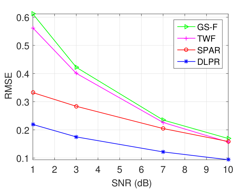
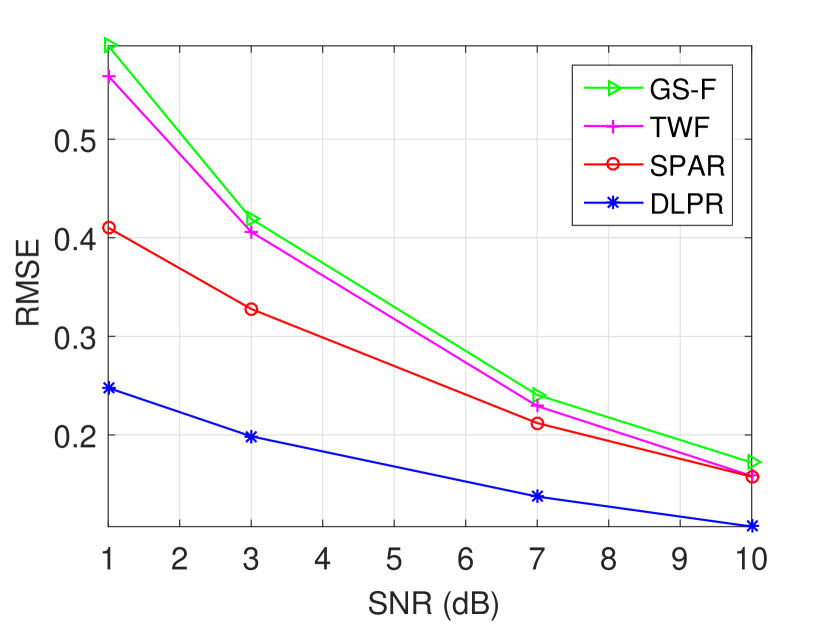
Experiments using real MRI interferograms are included in this section. The MRI interferograms 555The work was carried out on a 1.5 T GE Signa clinical scanner operating within Western General Hospital (WGH), University of Edinburgh. used in this section are obtained by scanning the human head region along side, top and front orientations as shown in Fig. 8. The complex-valued test images are generated by using each of these interferograms (figs. 8(a), 8(b), 8(c)) as the clean phase () with amplitude set to unity. These complex-valued images are self-similar, and thus its patches are well approximated by sparse representations over a learned dictionary. Hence we emphasize that although an optical set-up is being considered in our discussion, these MRI interferograms are relevant test images. In comparison to the synthetic data used in the previous experiments, these real interferograms do not have a well defined smooth structure and are highly challenging data for a PR experiment. Despite these challenges, DLPR remains to be a strong candidate proving its ability to retrieve real interferograms. The estimates for a highly noisy observation () are shown in Fig. 9. It can be qualitatively examined that DLPR estimates are much better in preserving the sharp details of the interferograms. This is clearly supported by the RMSE values. The results for other noise levels are shown in Fig. 10, in the form of a graph, from which we can arrive at the same conclusion. These experiments show the strong ability of DLPR to retrieve real phase data.
4.2 Gaussian Observation
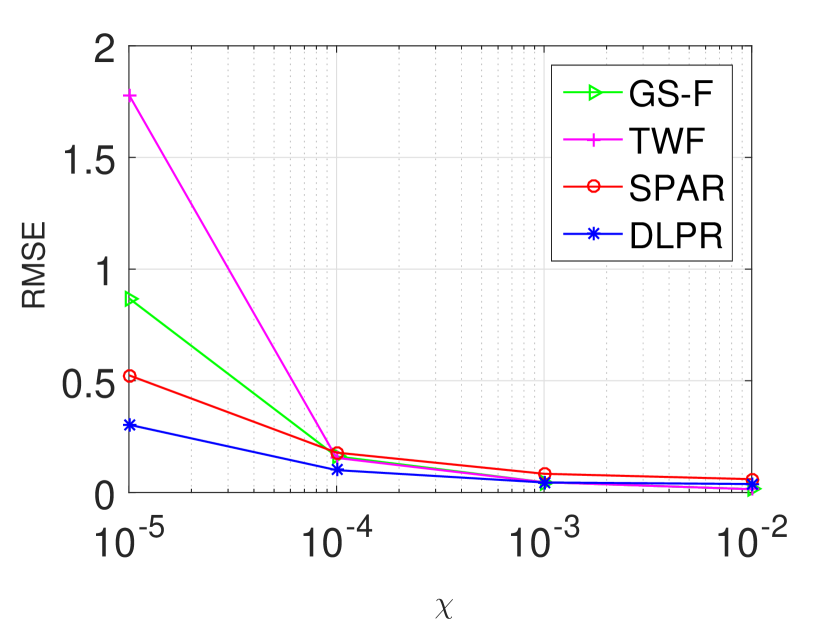
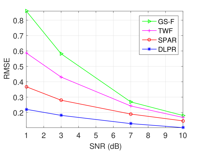
In this section, PR is conducted by considering a Gaussian observation model. Very low SNR values, i.e., is considered corresponding to highly to moderate noisy scenarios. In this section, we are not repeating all the experiments conducted for Possonian case. But the toughest experiments with real MRI interferograms are repeated. The results are shown in Fig. 11, which indicate that DLPR performs exceptionally well and beats it competitors with a good margin for all noise levels.
4.3 Prior-plugged DLPR for Class-specific Phase retrieval
DLPR algorithm 3 learns the dictionary iteratively and retrieves the phase from observed intensities. But in many practical applications, the phase to be recovered is known to belong to certain classes of images. In such applications, the clean images from the specific classes can be used to learn prior information and to enhance the PR process. Most of the PR methods that we discussed does not have the algorithmic structure to incorporate such priors. But DLPR, being a dictionary based method, opens the door to the exploitation of the learned prior. Algorithm 4, which we term as prior-plugged DLPR, is a modified version of the original DLPR Algorithm 3, obtained by skipping the online dictionary learning step and including the learned dictionary (prior) as input.
In this section, the class-specific phase retrieval using prior-plugged DLPR is illustrated using two experiments, the first one using simulated data and the second one using real data. In the first experiment, to learn the prior (dictionary), a Gaussian surface and its four quarters, as shown in Fig. 12(a), is considered. The C-ODL Algorithm 2 is used to learn the dictionary. PR is performed on a truncated Gaussian surface created by cutting off the alternate octants of a Gaussian surface, as shown in Fig. 12(b). We remark that the retrieval of this surface is quite challenging as it contains less connected areas and has a lot of sharp discontinuities. Though the prior and the testing surface are different, they belong to the same class of truncated Gaussians and share many identical regions.
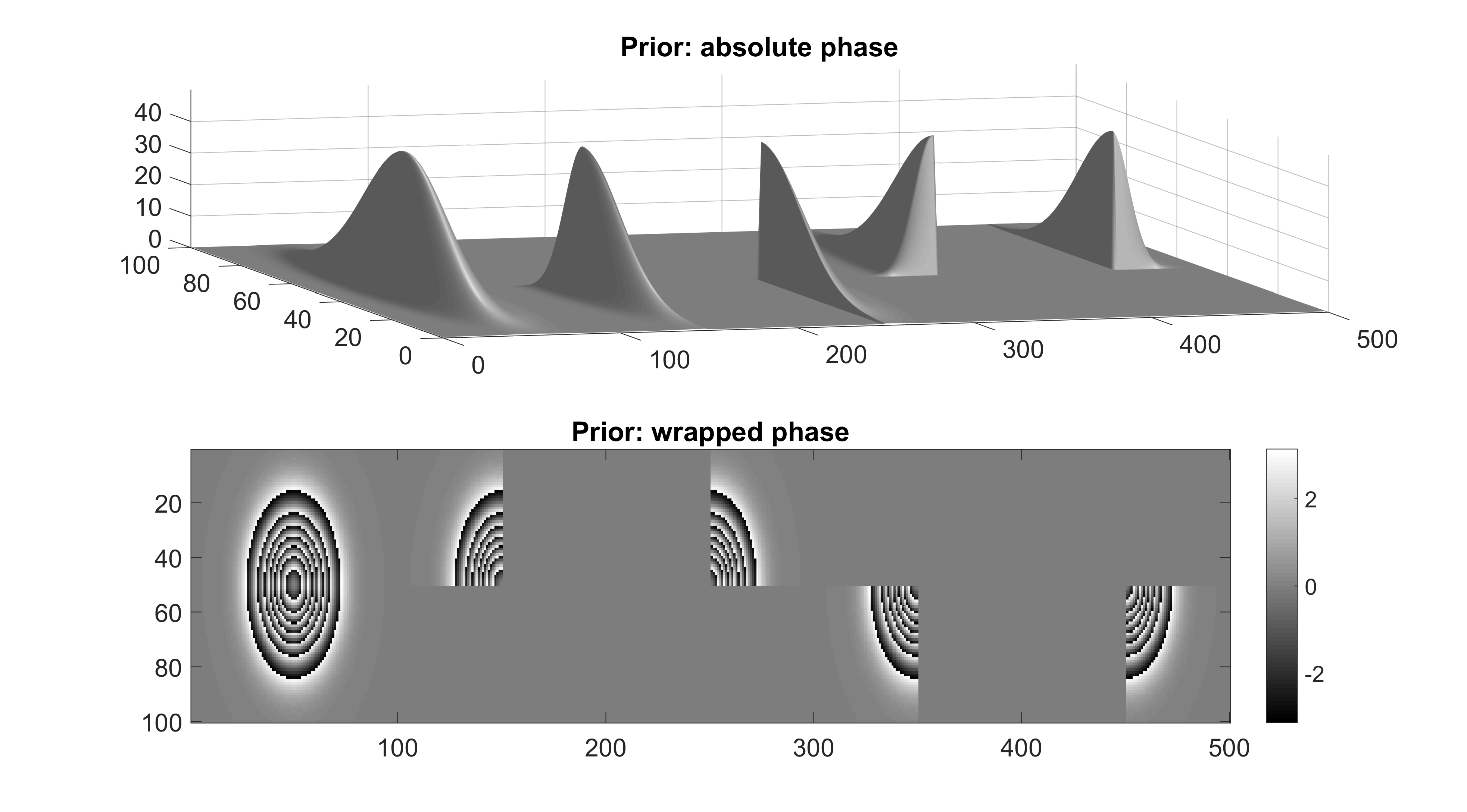
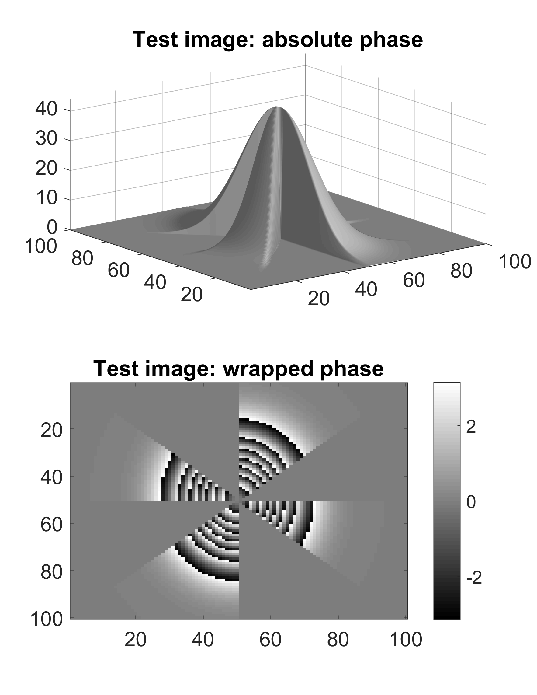
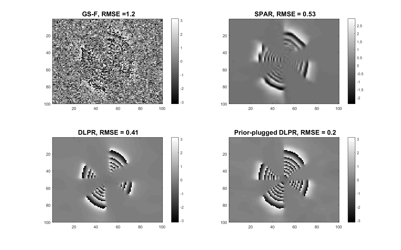
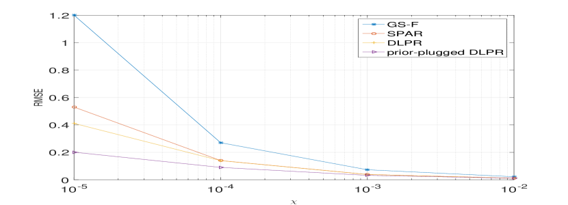
Fig. 13(a) shows the results for prior-plugged DLPR in comparison with GS-F, SPAR, and DLPR using very high Poissonian noise (). It is quite evident that the prior-plugged DLPR shows remarkable improvement by exploiting the learned prior. In comparison with the original DLPR, which does not use the prior, the prior-plugged DLPR has an improvement in RMSE by . The results for similar experiments by considering other noise levels are plotted in Fig. 13(b) in which prior-plugged DLPR beats all other methods, especially for the highly noisy cases.
The remarkable improvement in RMSE in the above experiment is due to the fact that both the prior-learning surface and the phase to be retrieved share many identical regions. But in practice this may not be true and we only have access to data from the same class. The phase to be retrieved need not possess regions exactly identical with the training images. To account this factor, we present a second experiment using real MRI data. The details of the data set 333The work was carried out on a 1.5 T GE Signa clinical scanner operating within Western General Hospital (WGH), University of Edinburgh. is shown in Fig. 14.
In this experiment, the MRI phase images obtained from four different persons are used. These images are the interferograms of the head region obtained through the scanning along front, side and top orientations. In the following experiment, a particular scanning orientation, say front view, is taken as a specific class. The dictionary is learned from the front view interferograms of person-1,2 and 3. This dictionary is used as the prior for retrieving the interferograms of the fourth person along front view. In the PR experiment, a very high Poissonian noise corresponding to () is considered. The experiment is repeated for other two scanning orientations, i.e., side view and top view. The result in terms of RMSE is given in Table 2. From the table, it is evident that prior-plugged DLPR is much better compared to SPAR, GS-F, and TWF and yields slightly better results compared to normal DLPR. We emphasis that in prior-plugged DLPR, the fourth person’s MRI phase image is retrieved just by using the dictionary learned from the scan images of the other three persons and still, the obtained results are better than the normal DLPR. This proves that prior-plugged DLPR is a powerful tool for class-specific phase retrieval applications.
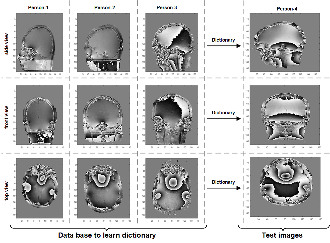
| RMSE | |||||
| Surf. | prior-plugged | ||||
| GS-F | TWF | SPAR | DLPR | DLPR | |
| Side view | 0.587 | 1.560 | 0.330 | 0.202 | 0.184 |
| Top view | 0.707 | 1.789 | 0.366 | 0.220 | 0.194 |
| Front view | 0.698 | 1.693 | 0.393 | 0.226 | 0.192 |
4.4 Complexity of DLPR
The complexity of DLPR is mainly defined by the dictionary learning and OMP steps. A theoretical analysis on this is beyond the scope of the work presented. However, we characterise the complexity by the time required to retrieve the phase. All the results presented in this paper are obtained through 20 iterations of DLPR and 50 iterations (as suggested by SPAR) of SPAR, GS-F, and TWF. We use MATLAB R2015b and computer with the processor Intel(R) Core(TM) i7-4790 CPU @3.60GHz, 16GB RAM. With the above mentioned number of iterations using an image of size under Poissonian noise (), the time required for phase retrieval is as follows: DLPR 77.6 sec, prior-pluged DLPR 23.6 sec, SPAR 15 sec, GS-F 0.43 sec, TWF 0.89 sec. It is to be noted that, in terms of time of convergence, DLPR lags behind SPAR due to its dictionary learning and sparse coding sub iterations that are computationally demanding.
5 Conclusion
Phase Retrieval from noisy intensity observations is addressed in this paper. A noisy optical system with wavefront modification is adopted for the discussion. The conventional PR algorithms fail to retrieve good quality phase images from noisy observations. To address this issue, a novel algorithm, termed as DLPR has been proposed in this paper. DLPR is an iterative algorithm developed under the alternating minimization framework and incorporates specially designed filters both at the sensor and the object plane of the optical imaging system. At the object plane, a sparse wavefront modeling using complex valued dictionary is done to obtain noise immunity. A second filtering mechanism is applied at the sensor plane aiming at additional noise suppression and is designed for Poissonian and for Gaussian observations. All the filters and optic propagation models are designed in a variational framework that maximizes the likelihood function and is aimed to iterate towards statistically optimal estimates.
The performance of the proposed algorithm is tested using challenging simulated and real data set. The state-of-the-art PR algorithms, namely SPAR, TWF, and GS-F, are used for performance comparisons. DLPR shows remarkable improvements over the conventional GS family and the recent TWF algorithm for highly noisy observations and its performance is quite competitive to BM3D-based SPAR. It is shown that DLPR beats SPAR for highly noisy observations. DLPR also has an added advantage of prior exploitation in class-specific phase retrieval over SPAR, which was empirically demonstrated. As a future work, we suggest further researches on dictionary-based phase retrieval to improve the convergence speed of the algorithm by exploiting fast dictionary and sparse coding techniques.
Investigation, J.P. K.; Methodology, V.K; Supervision, J.M.B and V.K; Validation, J.P. K; Writing – original draft, J.P. K ; Writing – review & editing, J.M.B. \fundingThe research leading to these results has received funding from the European Union’s H2020 Framework Programme (H2020-MSCA-ITN-2014) under grant agreement no 642685 MacSeNet. This work is also supported by the Portuguese Fundacão para a Ciência e Tecnologia (FCT) under grants UID/EEA/5008/2013 and Academy of Finland, project no. 287150, 2015-2019.
Acknowledgements.
The authors would like to thank Wajiha Bano, Institute for Digital Communications, University of Edinburgh, for providing the MRI data used in the experiment section of the manuscript. \conflictsofinterestThe authors declare no conflict of interest. The founding sponsors had no role in the design of the study; in the collection, analyses, or interpretation of data; in the writing of the manuscript, or in the decision to publish the results. \reftitleReferencesReferences
- Candes et al. (2013) Candes, E.; Eldar, Y.; Strohmer, T.; Voroninski, V. Phase Retrieval via Matrix Completion. SIAM Journal on Imaging Sciences 2013, 6, 199–225.
- Katkovnik (2017) Katkovnik, V. Phase retrieval from noisy data based on sparse approximation of object phase and amplitude. CoRR 2017, abs/1709.01071.
- Candès et al. (2015) Candès, E.; Li, X.; Soltanolkotabi, M. Phase Retrieval via Wirtinger Flow: Theory and Algorithms. IEEE Transactions on Information Theory 2015, 61, 1985–2007.
- Saleh and Teich (2007) Saleh, B.; Teich, M. Fundamentals of photonics; 2nd ed.; Wiley series in pure and applied optics, Wiley: New York, NY, 2007.
- Goodman (2005) Goodman, J. Introduction to Fourier optics. Introduction to Fourier optics, 3rd ed., by JW Goodman. Englewood, CO: Roberts & Co. Publishers, 2005 2005, 1.
- Sayre (1952) Sayre, D. Some implications of a theorem due to Shannon. Acta Crystallographica 1952, 5, 843.
- Millane (1990) Millane, R. Phase retrieval in crystallography and optics. J. Opt. Soc. Am. A 1990, 7, 394–411. doi:\changeurlcolorblack10.1364/JOSAA.7.000394.
- Harrison (1993) Harrison, R. Phase problem in crystallography. J. Opt. Soc. Am. A 1993, 10, 1046–1055.
- Bonse and Hart (1965) Bonse, U.; Hart, M. AN X-RAY INTERFEROMETER. Applied Physics Letters 1965, 6, 155–156.
- Petrakov (2003) Petrakov, A. X-ray phase-contrast method and its application to the study of blood vessels with a model object. Technical Physics 2003, 48, 607–611.
- Snigirev et al. (1995) Snigirev, A.; Snigireva, I.; Kohn, V.; Kuznetsov, S.; Schelokov, I. On the possibilities of x-ray phase contrast microimaging by coherent high energy synchrotron radiation. Review of Scientific Instruments 1995, 66, 5486–5492.
- Wilkins et al. (1996) Wilkins, S.; Gureyev, T.; Gao, D.; Pogany, A.; Stevenson, A. Phase-contrast imaging using polychromatic hard X-rays. Nature 1996, pp. 335––338. doi:\changeurlcolorblackdoi:10.1038/384335a0.
- Pfeiffer et al. (2006) Pfeiffer, F.; Weitkamp, T.; Bunk, O.; David, C. Phase retrieval and differential phase-contrast imaging with low-brilliance X-ray sources. Nature 2006, pp. 258––261. doi:\changeurlcolorblackdoi:10.1038/nphys265.
- Miao et al. (59:387-410, 2008) Miao, J.; Ishikawa, T.; Shen, Q.; .; Earnest., T. Extending x-ray crystallography to allow the imaging of noncrystalline materials, cells, and single protein complexes. Annu. Rev. Phys. Chem. 59:387-410, 2008.
- Walther (1963) Walther, A. The Question of Phase Retrieval in Optics. Optica Acta: International Journal of Optics 1963, 10, 41–49.
- Rabiner and Juang (1993) Rabiner, L.; Juang, B. Fundamentals of Speech Recognition; Prentice-Hall, Inc.: Upper Saddle River, NJ, USA, 1993.
- Balan et al. (2006) Balan, R.; Casazza, P.; Edidin, D. On signal reconstruction without phase. Applied and Computational Harmonic Analysis 2006, 20, 345 – 356.
- Dainty and Fienup (1987) Dainty, J.; Fienup, J. Phase retrieval and image reconstruction for astronomy. Image Recovery: Theory and Applicatio 1987, pp. 231–275.
- Chai et al. (2011) Chai, A.; Moscoso, M.; Papanicolaou, G. Array imaging using intensity-only measurements. Inverse Problems 2011, 27, 015005.
- Demanet and Jugnon (2017) Demanet, L.; Jugnon, V. Convex Recovery From Interferometric Measurements. IEEE Transactions on Computational Imaging 2017, 3, 282–295.
- Stefik (1978) Stefik, M. Inferring DNA structures from segmentation data. Artificial Intelligence 1978, 11, 85 – 114. Applications to the Sciences and Medicine.
- Bunk et al. (63(4) Bunk, O.; Diaz, A.; Pfeiffer, F.; David, C.; Schmitt, B.; Satapathy, D.; Veen, J. Diffractive imaging for periodic samples: retrieving one-dimensional concentration profiles across microfluidic channels. Acta Crystallographica Section A: Foundations of Crystallography 63(4): 306-314, 2007.
- Baykal (2004) Baykal, B. Blind channel estimation via combining autocorrelation and blind phase estimation. IEEE Transactions on Circuits and Systems I: Regular Papers 2004, 51, 1125–1131.
- Corbett (2006) Corbett, J. The pauli problem, state reconstruction and quantum-real numbers. Reports on Mathematical Physics 2006, 57, 53 – 68.
- Reichenbach (1965) Reichenbach, H. Philosophic foundations of quantum mechanics.; University of California Pr, 1965.
- Heinosaari et al. (2013) Heinosaari, T.; Luca, M.; M. Wolf, . Quantum Tomography under Prior Information. Communications in Mathematical Physics 2013, 318, 355–374.
- Ahmed et al. (2014) Ahmed, A.; Recht, B.; Romberg, J. Blind Deconvolution Using Convex Programming. IEEE Transactions on Information Theory 2014, 60, 1711–1732.
- (28) Ranieri, J.; Chebira, A.; Lu, Y.; Vetterli, M. Phase Retrieval for Sparse Signals: Uniqueness Conditions.
- Dierolf et al. (2010) Dierolf, M.; Menzel, A.; Thibault, P.; Schneider, P.; Kewish, C.; Wepf, R.; Bunk, O.; Pfeiffer, F. Ptychographic X-ray computed tomography at the nanoscale. Nature 2010, pp. 436––439.
- Bianchi et al. (60 (2002) Bianchi, G.; Segala, F.; Volcic, A. The solution of the covariogram problem for plane convex bodies. J. Differential Geom. 60 (2002), pp. 177––198.
- Gerchberg and Saxton (1972) Gerchberg, R.; Saxton, W. A Practical Algorithm for the Determination of Phase from Image and Diffraction Plane Pictures. OPTIK 1972, 35, 237–246.
- Guo et al. (2015) Guo, C.; Liu, S.; Sheridan, J. Iterative phase retrieval algorithms I: optimization. Appl. Opt. 2015, 54, 4698–4708.
- Yang et al. (1994) Yang, G.; Dong, B.; Gu, B.; Zhuang, J.; Ersoy, O. Gerchberg–Saxton and Yang–Gu algorithms for phase retrieval in a nonunitary transform system: a comparison. Appl. Opt. 1994, 33, 209–218.
- Fienup (1982) Fienup, J. Phase retrieval algorithms: a comparison. Appl. Opt. 1982, 21, 2758–2769.
- Lane (1991) Lane, R. Phase Retrieval Using Conjugate Gradient Minimization. J. Modern Optics 1991, 38, 1797–1813.
- Chen and Candes (2015) Chen, Y.; Candes, E. Solving Random Quadratic Systems of Equations Is Nearly as Easy as Solving Linear Systems. In Advances in Neural Information Processing Systems 28; Curran Associates, Inc., 2015; pp. 739–747.
- Waldspurger et al. (2015) Waldspurger, I.; Aspremont, A.; Mallat, S. Phase recovery, MaxCut and complex semidefinite programming. Mathematical Programming 2015, 149, 47–81. doi:\changeurlcolorblack10.1007/s10107-013-0738-9.
- Bahmani and Romberg (2017) Bahmani, S.; Romberg, J. A flexible convex relaxation for phase retrieval. Electron. J. Statist. 2017, 11, 5254–5281.
- Kishore et al. (2015) Kishore, J.; Eldar, Y.; Hassibi, B. Phase Retrieval: An Overview of Recent Developments. CoRR 2015, abs/1510.07713.
- Nugent et al. (2003) Nugent, K.; Peele, A.; Chapman, H.; Mancuso, A. Unique Phase Recovery for Nonperiodic Objects. Phys. Rev. Lett. 2003, 91, 203902.
- Johnson et al. (2008) Johnson, I.; Jefimovs, K.; Bunk, O.; David, C.; Dierolf, M.; Gray, J.; Renker, D.; Pfeiffer, F. Coherent Diffractive Imaging Using Phase Front Modifications. Physical Review Letters 2008, 100.
- Candes et al. (2015) Candes, E.; Li, X.; Soltanolkotabi, M. Phase retrieval from coded diffraction patterns. Applied and Computational Harmonic Analysis 2015, 39, 277 – 299.
- Zhang et al. (2007) Zhang, F.; Pedrini, G.; Osten, W. Phase retrieval of arbitrary complex-valued fields through aperture-plane modulation. Phys. Rev. A 2007, 75, 043805.
- Elad (2010) Elad, M. Sparse and Redundant Representations: From Theory to Applications in Signal and Image Processing, 1st ed.; Springer Publishing Company, Incorporated, 2010.
- Jaganathan et al. (2017) Jaganathan, K.; Oymak, S.; Hassibi, B. Sparse Phase Retrieval: Uniqueness Guarantees and Recovery Algorithms. IEEE Transactions on Signal Processing 2017, 65, 2402–2410.
- Shechtman et al. (2014) Shechtman, Y.; Beck, A.; Eldar, Y. GESPAR: Efficient Phase Retrieval of Sparse Signals. IEEE Transactions on Signal Processing 2014, 62, 928–938.
- Dabov et al. (2006) Dabov, K.; Foi, A.; Katkovnik, V.; Egiazarian, K. Image denoising with block-matching and 3D filtering. Proc.SPIE 2006, 6064.
- Afonso et al. (2015) Afonso, T.; Almeida, M.; Figueiredo, M. Single-frame Image Denoising and Inpainting Using Gaussian Mixtures. Proceedings of the International Conference on Pattern Recognition Applications and Methods, 2015, Vol. 2, pp. 283–288.
- Elad and Aharon (2006) Elad, M.; Aharon, M. Image denoising via sparse and redundant representations over learned dictionaries. IEEE Transactions on Image processing 2006, 15, 3736–3745.
- Dabov et al. (2007) Dabov, K.; Foi, A.; Katkovnik, V.; Egiazarian, K. Image Denoising by Sparse 3D Transform-Domain Collaborative Filtering. IEEE Transactions on Image Processing 2007, 16, 2080–2095. doi:\changeurlcolorblack10.1109/TIP.2007.901238.
- Li et al. (2014) Li, S.; Cao, Q.; Chen, Y.; Hu, Y.; Luo, L.; Toumoulin, C. Dictionary learning based sinogram inpainting for CT sparse reconstruction. Optik - International Journal for Light and Electron Optics 2014, 125, 2862 – 2867.
- Deledalle et al. (2011) Deledalle, C.; Denis, L.; Tupin, F. NL-InSAR: Nonlocal Interferogram Estimation. IEEE Transactions on Geoscience and Remote Sensing 2011, 49, 1441–1452.
- Hongxing et al. (2015) Hongxing, H.; Bioucas-Dias, J.; Katkovnik, V. Interferometric Phase Image Estimation via Sparse Coding in the Complex Domain. IEEE Transactions on Geoscience and Remote Sensing 2015, 53, 2587–2602.
- Joshin and Bioucas-Dias (2017) Joshin, K.; Bioucas-Dias, J. Patch-based Interferometric Phase Estimation via Mixture of Gaussian Density Modelling & Non-local Averaging in the Complex Domain. British Machine Vision Conference, 2017.
- Katkovnik and Egiazarian (2017) Katkovnik, V.; Egiazarian, K. Sparse phase imaging based on complex domain nonlocal BM3D techniques. Digital Signal Processing 2017, 63, 72 – 85.
- Bioucas-Dias and Valadao (2007) Bioucas-Dias, J.; Valadao, G. Phase Unwrapping via Graph Cuts. IEEE Transactions on Image Processing 2007, 16.
- Tillmann et al. (2016) Tillmann, A.; Eldar, Y.; Mairal, J. DOLPHIn-Dictionary Learning for Phase Retrieval. IEEE Transactions on Signal Processing 2016, 64, 6485–6500.
- Katkovnik et al. (2014) Katkovnik, V.; Egiazarian, K.; Bioucas-Dias, J. Phase imaging via sparse coding in the complex domain based on high-order SVD and nonlocal BM3D techniques. 2014 IEEE International Conference on Image Processing (ICIP), 2014, pp. 4587–4591. doi:\changeurlcolorblack10.1109/ICIP.2014.7025930.
- Soulez et al. (2016) Soulez, F.; Thiébaut, E.; Schutz, A.; Ferrari, A.; Courbin, F.; Unser, M. Proximity operators for phase retrieval. Appl. Opt. 2016, 55, 7412–7421.
- Raginsky et al. (2010) Raginsky, M.; Willett, R.; Harmany, Z.; Marcia, R. Compressed Sensing Performance Bounds Under Poisson Noise. IEEE Transactions on Signal Processing 2010, 58, 3990–4002.
- Salmon et al. (2014) Salmon, J.; Harmany, Z.; Deledalle, C.; Willett, R. Poisson Noise Reduction with Non-local PCA. Journal of Mathematical Imaging and Vision 2014, 48, 279–294.
- Harmany et al. (2010) Harmany, Z.; Marcia, R.; Willett, R. Sparsity-regularized photon-limited imaging. 2010 IEEE International Symposium on Biomedical Imaging: From Nano to Macro, 2010, pp. 772–775.
- Adali et al. (2011) Adali, T.; Schreier, P.; Scharf, L. Complex-Valued Signal Processing: The Proper Way to Deal With Impropriety. IEEE Transactions on Signal Processing 2011, 59, 5101–5125.
- Rakotomamonjy (2013) Rakotomamonjy, A. Applying alternating direction method of multipliers for constrained dictionary learning. Neurocomputing 2013, 106, 126 – 136.
- Combettes and Pesquet (2011) Combettes, P.; Pesquet, J. Proximal splitting methods in signal processing. In Fixed-point algorithms for inverse problems in science and engineering; Springer, 2011; pp. 185–212.
- Katkovnik and Bioucas-Dias (2014) Katkovnik, V.; Bioucas-Dias, J. Wavefront reconstruction in phase-shifting interferometry via sparse coding of amplitude and absolute phase. J. Opt. Soc. Am. A 2014, 31, 1801–1810.
- Natarajan (1995) Natarajan, B. Sparse Approximate Solutions to Linear Systems. SIAM Journal on Computing 1995, 24, 227–234.
- Tibshirani (1994) Tibshirani, R. Regression Shrinkage and Selection Via the Lasso. Journal of the Royal Statistical Society, Series B 1994, 58, 267–288.
- Chen et al. (1998) Chen, S.; Donoho, D.; Saunders, M. Atomic Decomposition by Basis Pursuit. SIAM Journal on Scientific Computing 1998, 20, 33–61.
- Mairal et al. (2009) Mairal, J.; Bach, F.; Ponce, J.; Sapiro, G. Online Dictionary Learning for Sparse Coding. Proceedings of the 26th Annual International Conference on Machine Learning; ACM: New York, NY, USA, 2009; ICML ’09, pp. 689–696.
- Pati et al. (1993) Pati, Y.; Rezaiifar, R.; Krishnaprasad, P. Orthogonal matching pursuit: recursive function approximation with applications to wavelet decomposition. Proceedings of 27th Asilomar Conference on Signals, Systems and Computers, 1993, pp. 40–44 vol.1.
- Efron et al. (2004) Efron, B.; Hastie, T.; Johnstone, I.; Tibshirani, R. Least angle regression. Annals of Statistics 2004, 32, 407–499.
- Katkovnik and Astola (2012) Katkovnik, V.; Astola, J. Phase retrieval via spatial light modulator phase modulation in 4f optical setup: numerical inverse imaging with sparse regularization for phase and amplitude. J. Opt. Soc. Am. A 2012, 29, 105–116.