Good Initializations of Variational Bayes for Deep Models

Abstract

Stochastic variational inference is an established way to carry out approximate Bayesian inference for deep models. While there have been effective proposals for good initializations for loss minimization in deep learning, far less attention has been devoted to the issue of initialization of stochastic variational inference. We address this by proposing a novel layer-wise initialization strategy based on Bayesian linear models. The proposed method is extensively validated on regression and classification tasks, including Bayesian DeepNets and ConvNets, showing faster and better convergence compared to alternatives inspired by the literature on initializations for loss minimization.

1 Introduction

Deep Neural Networks (dnns) and Convolutional Neural Networks (cnns) have become the preferred choice to tackle various supervised learning problems, such as regression and classification, due to their ability to model complex problems and the mature development of regularization techniques to control overfitting (LeCun et al., 2015; Srivastava et al., 2014). There has been a recent surge of interest in the issues associated with their overconfidence in predictions, and proposals to mitigate these (Guo et al., 2017; Kendall & Gal, 2017; Lakshminarayanan et al., 2017). Bayesian techniques offer a natural framework to deal with such issues, but they are characterized by computational intractability (Bishop, 2006; Ghahramani, 2015).

A popular way to recover tractability is to use variational inference (Jordan et al., 1999). In variational inference, an approximate posterior distribution is introduced and its parameters are adapted by optimizing a variational objective, which is a lower bound to the marginal likelihood. The variational objective can be written as the sum of an expectation of the log-likelihood under the approximate posterior and a regularization term which is the negative Kullback-Leibler (kl) divergence between the approximating distribution and the prior over the parameters. Stochastic Variational Inference (svi) offers a practical way to carry out stochastic optimization of the variational objective. In svi, stochasticity is introduced with a doubly stochastic approximation of the expectation term, which is unbiasedly approximated using Monte Carlo and by selecting a subset of the training points (mini-batching) (Graves, 2011; Kingma & Welling, 2014).

Figure 1: Due to poor initialization (left) svi fails to converge even after $600+$ epochs (${\textsc{rmse}}=0.613$, ${\textsc{mnll}}=29.4$) while with our i-blm (right) svi easily recovers the function after few epochs (${\textsc{rmse}}=0.315$, ${\textsc{mnll}}=-5.8$). The architecture has three hidden layers with $500$ neurons each, and uses the tanh activation function.

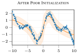
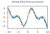
While svi is an attractive and practical way to perform approximate inference for dnns, there are limitations. For example, the form of the approximating distribution can be too simple to accurately approximate complex posterior distributions (Ha et al., 2016; Ranganath et al., 2015; Rezende & Mohamed, 2015). Furthermore, svi increases the number of optimization parameters compared to optimizing model parameters through, e.g., loss minimization; for example, a fully factorized Gaussian posterior over model parameters doubles the number of parameters in the optimization compared to loss minimization. This has motivated research into other ways to perform approximate Bayesian inference for dnns by establishing connections between variational inference and dropout (Gal & Ghahramani, 2016a, b; Gal et al., 2017).

The development of a theory to fully understand the optimization landscape of dnns and cnns is still in its infancy (Dziugaite & Roy, 2017) and most works have focused on the practical aspects characterizing the optimization of their parameters (Duchi et al., 2011; Kingma & Ba, 2015; Srivastava et al., 2014). If this lack of theory is apparent for optimization of model parameters, this is even more so for the understanding of the optimization landscape of the objective in variational inference, where variational parameters enter in a nontrivial way in the objective (Graves, 2011; Rezende et al., 2014). Initialization plays a huge role in the convergence of svi; the illustrative example in Figure 1 shows how a poor initialization can prevent svi to converge to good solutions in short amount of time even for simple problems. The problem is even more severe for complex architectures, such as the ones that we discuss in the experiments; for example, svi systematically converges to trivial solutions (posterior equal to the prior) when applied to cnns, due to the difficulty in initializing variational parameters sensibly.

In this work, we focus on this issue affecting svi for dnns and cnns. While there is an established literature on ways to initialize model parameters of dnns when minimizing its loss (Glorot & Bengio, 2010; Saxe et al., 2013; Mishkin & Matas, 2015), to the best of our knowledge, there is no study that systematically tackle this issue for svi for Bayesian dnns and cnns. Inspired by the literature on residual networks (He et al., 2016) and greedy initialization of dnns (Bengio et al., 2006; Mishkin & Matas, 2015), we propose Iterative Bayesian Linear Modeling (i-blm), which is an initialization strategy for svi grounded on Bayesian linear modeling. Iterating from the first layer, i-blm initializes the posteriors at layer $l$ by learning Bayesian linear models which regress from the input, propagated up to layer $l$, to the labels.

We show how i-blm can be applied in a scalable way and without considerable overhead to regression and classification problems, and how it can be applied to initialize svi not only for dnns but also for cnns. Through a series of experiments, we demonstrate that i-blm leads to faster convergence compared to other initalizations inspired by the work on loss minimization for dnns. Furthermore, we show that i-blm makes it possible for svi with a Gaussian approximation applied to cnns to compete with Monte Carlo Dropout (mcd; Gal & Ghahramani (2016b)) and noisy natural gradients (noisy-kfac; Zhang et al. (2018)), which are state-of-art methods to perform approximate inference for cnns. In all, thanks to the proposed initialization, we make it possible to reconsider Gaussian svi for dnns and cnns as a valid competitor to mcd and noisy-kfac, as well as highlight the limitations of svi with a Gaussian posterior in applications involving cnns.

In summary, in this work we make the following contributions: (1) we propose a novel way to initialize svi for dnns based on Bayesian linear models; (2) we show how this can be done for regression and classification; (3) we show how to apply our strategy to cnns; (4) we empirically demonstrate that our proposal allows us to achieve performance superior to other initializations of svi inspired by the literature on loss minimization; (5) for the first time, we achieve state-of-the-art performance with Gaussian svi for large-scale cnns.

2 Related Work

The problem of initialization of weights and biases in dnns for gradient-based loss minimization has been extensively tackled in the literature since early breakthroughs in the field (Rumelhart et al., 1986; Baldi & Hornik, 1989). LeCun (1998) is one of the seminal papers discussing practical tricks to achieve an efficient loss minimization through back-propagation.

More recently, Bengio et al. (2006) propose a greedy layer-wise unsupervised pre-training that proved to help optimization and generalization. A justification can be found in Erhan et al. (2010), where the authors show that pre-training can act as regularization; by initializing the parameters in a region corresponding to a better basin of attraction for the optimization procedure, the model can reach a better local minimum and increase its generalization capabilities. Glorot & Bengio (2010) propose a simple way to estimate the variance for random initialization of weights that makes it possible to avoid saturation both in forward and back-propagation steps. Another possible strategy can be found in Saxe et al. (2013), that investigate the dynamics of gradient descend optimization, and propose an initialization based on random orthogonal initial conditions. This algorithm takes a weight matrix filled with Gaussian noise, decomposes it to orthonormal basis using a singular value decomposition and replaces the weights with one of the components. Building on this work, Mishkin & Matas (2015) propose a data-driven weight initialization by scaling the orthonormal matrix of weights to make the variance of the output as close to one as possible.

Variational inference addresses the problem of intractable Bayesian inference by reinterpreting inference as an optimization problem. Its origins can be tracked back to early works in MacKay (1992); Hinton & van Camp (1993); Neal (1997). More recently, Graves (2011) proposes a practical way to carry out variational inference using stochastic optimization (Duchi et al., 2011; Zeiler, 2012; Sutskever et al., 2013; Kingma & Ba, 2015). Kingma & Welling (2014) propose a reparameterization trick that allows for the optimization of the variational lower bound through automatic differentiation. To decrease the variance of stochastic gradients, which impacts convergence speed, this work is extended using the so-called local reparameterization trick, where the sampling from the approximate posterior over model parameters is replaced by the sampling from the resulting distribution over the dnn units (Kingma et al., 2015).

In the direction of finding richer posterior families for variational inference, we mention the works on Normalizing Flows (Rezende & Mohamed, 2015; Kingma et al., 2016; Louizos & Welling, 2017; Huang et al., 2018). Alternatives can be found in Stein variational inference (Liu & Wang, 2016), quasi-Monte Carlo variational inference (Buchholz et al., 2018), variational boosting (Miller et al., 2017), noisy natural gradients (Zhang et al., 2018) and matrix Gaussian posterior (Louizos & Welling, 2016b).

To the best of our knowledge, there is no study that either empirically or theoretically addresses the problem of initialization of parameters for svi; we could only find a mention of this in Krishnan et al. (2018) for variational autoencoders. We aim to fill this gap by proposing a novel way to initialize parameters in svi for probabilistic deep models.

3 Preliminaries

In this section we introduce some background material on Bayesian dnns and svi.

Bayesian Deep Neural Networks

Bayesian dnns are statistical models whose parameters (weights and biases) are assigned a prior distribution and inferred using Bayesian inference techniques. Bayesian dnns inherit the modeling capacity of dnns while allowing for quantification of uncertainty in model parameters and predictions. Considering an input $\mathbf{x}\in\mathbb{R}^{D_{\mathrm{in}}}$ and a corresponding output $\mathbf{y}\in\mathbb{R}^{D_{\mathrm{out}}}$, the relation between inputs and outpus can be seen as a composition of nonlinear vector-valued functions $\mathbf{f}^{(l)}$ for each hidden layer $(l)$

$$\mathbf{y}=\mathbf{f}(\mathbf{x})=\left(\mathbf{f}^{(L-1)}\circ\ldots\circ\mathbf{f}^{(0)}\right)(\mathbf{x})\,.$$ (1)

Let $\mathbf{W}$ be a collection of all model parameters (weights and biases) $W^{(l)}$ at all hidden layers. Each neuron computes its output as

$$f_{i}^{(l)}=\phi(\mathbf{w}_{i}^{(l)^{\top}}\mathbf{f}^{(l-1)})\,,$$ (2)

where $\phi(\cdot)$ denotes a so-called activation function which introduces a nonlinearity at each layer. Note that we absorbed the biases in $\mathbf{w}$.

Given a prior over $\mathbf{W}$, the objective of Bayesian inference is to find the posterior distribution over all model parameters $\mathbf{W}$ using the available input data $X=\{\mathbf{x}_{1},\ldots,\mathbf{x}_{n}\}$ associated with labels $Y=\{\mathbf{y}_{1},\ldots,\mathbf{y}_{n}\}$

$$p(\mathbf{W}|X,Y)=\frac{p(Y|X,\mathbf{W})p(\mathbf{W})}{p(Y|X)}\,.$$ (3)

Bayesian inference for dnns is analytically intractable and it is necessary to resort to approximations. One way to recover tractability is through the use of variational inference techniques as described next.

Stochastic Variational Inference

In variational inference, we introduce a family of distributions $q_{\boldsymbol{\theta}}(\mathbf{W})$, parameterized through $\boldsymbol{\theta}$, and attempt to find an element of this family which is as close to the posterior distribution of interest as possible (Jordan et al., 1999). This can be formulated as a minimization with respect to $\boldsymbol{\theta}$ of the kl divergence (Kullback, 1959) between the elements of the family $q_{\boldsymbol{\theta}}(\mathbf{W})$ and the posterior:

$$q_{\tilde{\boldsymbol{\theta}}}(\mathbf{W})=\arg\min_{\boldsymbol{\theta}}\{{{\textsc{kl}}}\left(q_{\boldsymbol{\theta}}(\mathbf{W})||p(\mathbf{W}|X,Y)\right)\}\,.$$ (4)

Simple manipulations allow us to rewrite this expression as the negative lower bound (nelbo) to the marginal likelihood of the model (see supplementary material)

$${\textsc{nelbo}}={\textsc{nll}}+{{\textsc{kl}}}\left(q_{\boldsymbol{\theta}}(\mathbf{W})||p(\mathbf{W})\right)\,,$$ (5)

where the first term is the expected negative log-likelihood ${\textsc{nll}}=\mathbb{E}_{q_{\boldsymbol{\theta}}}\left[-\log p(Y|X,\mathbf{W})\right]$, and the second term acts as regularizer, penalizing distributions $q_{\boldsymbol{\theta}}$ that deviate too much from the prior. When the likelihood factorizes across data points, we can unbiasedly estimate the expectation term randomly selecting a mini-batch $\mathcal{B}$ of $m$ out of $n$ training points

$${\textsc{nll}}\approx-\frac{n}{m}\sum_{\mathbf{x},\mathbf{y}\in\mathcal{B}}\mathbb{E}_{q_{\boldsymbol{\theta}}}\log p(\mathbf{y}|\mathbf{x},\mathbf{W})\,.$$ (6)

Each term in the sum can be further unbiasedly estimated using $N_{\mathrm{MC}}$ Monte Carlo samples as

$$\mathbb{E}_{q_{\boldsymbol{\theta}}}\log p(\mathbf{y}|\mathbf{x},\mathbf{W})=\frac{1}{N_{\mathrm{MC}}}\sum_{i=1}^{N_{\mathrm{MC}}}\log p(\mathbf{y}|\mathbf{x},\mathbf{W}_{i})\,,$$ (7)

where $\mathbf{W}_{i}\sim q_{\boldsymbol{\theta}}(\mathbf{W})$. Following Kingma & Welling (2014), each sample $\mathbf{W}_{i}$ is constructed using the reparameterization trick, which allows to obtain a deterministic dependence of the nelbo w.r.t. $\boldsymbol{\theta}$. Alternatively, it is possible to determine the distribution of the dnn units $f_{i}^{(l)}$ before activation from $q_{\boldsymbol{\theta}}(\mathbf{W})$. This trick, known as the local reparameterization trick, allows one to considerably reduce the variance of the stochastic gradient w.r.t. $\boldsymbol{\theta}$ and achieve faster convergence as shown by Kingma et al. (2015).

4 Proposed Method

Figure 2: Visual representation of the proposed method for initialization. In (a) and (b), we learn two Bayesian linear models, whose outputs are used in (c) to infer the following layer.

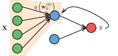
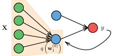
In this section, we introduce our proposed Iterative Bayesian Linear Model (i-blm) initialization for svi. We first introduce i-blm for regression with dnns, and we then show how this can be extended to classification and to cnns.

1

Inputs : Model $M$, Dataset $D$

2

3foreach layer in $M$ do

4      foreach outfeature in $layer$ do

5            $X,Y\leftarrow$ next batch in $D$;

6             propagate $X$;

7             $X_{\texttt{BLM}}\leftarrow$ output of previous layer;

8             if $layer$ is convolutional then $\triangleright$ ref 4.4

9                  $X_{\texttt{BLM}}\leftarrow$ patch extraction($X_{\texttt{BLM}}$);

10                  

11            if $likelihood$ is classification then $\triangleright$ ref 4.3

12                   $\text{var}(Y_{\texttt{BLM}})\leftarrow\log{[(Y+\alpha)^{-1}+1]}$;

13                   $\text{mean}(Y_{\texttt{BLM}})\leftarrow\log{(Y+\alpha)-\text{var}(Y_{\texttt{BLM}})/2}$;

14                  

15            else

16                   $Y_{\texttt{BLM}}\leftarrow Y$;

17                  

            $p(\mathbf{w}|X,Y)\leftarrow$ BLM($X_{\texttt{BLM}}$,$Y_{\texttt{BLM}}$) ;

              $\triangleright$ ref 4.1

             $q(\mathbf{w})\leftarrow$ best approx. of $p(\mathbf{w}|X,Y)$ ;

              $\triangleright$ ref 4.2

18            

Algorithm 1 Sketch of the i-blm Initializer

4.1 Initialization of DNNs for Regression

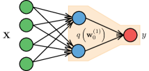
In order to initialize the weights of dnns, we proceed iteratively as follows. Before applying the nonlinearity through the activation function, each layer in a Bayesian dnn can be seen as multivariate Bayesian linear regression model. We use this observation as an inspiration to initialize svi as follows. Starting from the first layer, we can set the parameters of $q(W^{(0)})$ by running Bayesian linear regression with inputs $X$ and labels $Y$. After this, we initialize the approximate posterior over the weights at the second layer $q(W^{(1)})$ by running Bayesian linear regression with inputs $X=\Phi(X\tilde{W}^{(0)})$ and labels $Y$. Here, $\Phi(\cdot)$ denotes the elementwise application of the activation function to the argument, whereas $\tilde{W}^{(0)}$ is a sample from $q(W^{(0)})$. We then proceed iteratively in the same way up to the last layer. Figure 2 gives an illustration of the proposed method for a simple architecture.

The intuition behind i-blm is as follows. If one layer is enough to capture the complexity of a regression task, we expect to be able to learn an effective mapping right after the initialization of the first layer. In this case, we also expect that the mapping at the next layers implements simple transformations, close to the identity. Learning a set of weights with these characteristics starting from a random initialization is extremely hard; this motivated the work in He et al. (2016) that proposed the residual network architecture. Our i-blm initialization takes this observation as an intuition to initialize svi for general deep models.

From a complexity point of view, denoting by $h^{(l)}$ the number of output neurons at layer $(l)$, this is equivalent to $h^{(l)}$ univariate Bayesian linear models. Instead of using the entire training set to learn the linear models, each one of these is inferred based on a random mini-batch of data, whose inputs are propagated through the previous layers. The complexity of i-blm is linear in the batch size and cubic in the number of neurons to be initialized. Later on in this Section, we will provide an evaluation of the effect of batch size and a timing profiling of i-blm.

4.2 From the Bayesian linear model posterior to the variational approximation

The proposed i-blm initialization of variational parameters can be used with any choice for the form of the approximate posterior. The exact posterior of Bayesian linear regression is not factorized, so one needs to match this with the form of the chosen approximate posterior. For simplicity of notation, let $\mathbf{w}$ be the parameters of interest in Bayesian linear regression for a given output $\mathbf{y}=Y_{\cdot i}$. We can formulate this problem by minimizing the kl divergence from $q(\mathbf{w})$ to the actual posterior $p(\mathbf{w}|X,\mathbf{y})$. In the case of a fully factorized approximate posterior over the weights $q(W^{(l)})=\prod_{ij}q_{ij}(W^{(l)})$, this minimization can be done analytically. This results in the mean being equal to the mean of $p(\mathbf{w}|X,\mathbf{y})$ and the variances $(s_{i}^{2})^{-1}=\Sigma^{-1}_{ii}$; see the supplementary material for the full derivation. Similar results can be also obtained for different posterior distributions, such as Gaussian posteriors with full or low-rank covariance, or matrix-variate Gaussian posteriors (Louizos & Welling, 2016a).

4.3 Initialization for Classification

In this section we show how our proposal can be extended to $k$-class classification problems. We assume a one-hot encoding of the labels, so that $Y$ is an $n\times k$ matrix of zeros and ones (one for each row of $Y$). Recently, it has been shown that it is possible to obtain an accurate modeling of the posterior over classification functions by applying regression on a transformation of the labels (Milios et al., 2018). This is interesting because it allows us to apply Bayesian linear regression as before in order to initialize svi for dnns.

The transformation of the labels is based on the formalization of a simple intuition, which is the inversion of the softmax transformation. One-hot encoded labels are viewed as a set of parameters of a degenerate Dirichlet distribution. We resolve the degeneracy of the Dirichlet distribution by adding a small regularization, say $\alpha=0.01$, to the parameters. At this point, we leverage the fact that Dirichlet distributed random variables can be constructed as a ratio of Gamma random variables, that is, if $x_{i}\sim\mathrm{Gamma}(a_{i},b)$, then $\frac{x_{i}}{\sum_{j}x_{j}}\sim\mathrm{Dir}(\mathbf{a})$. We can then approximate the Gamma random variables with log-Normals by moment matching. By doing so, we obtain a representation of the labels which allows us to use standard regression with a Gaussian likelihood, and which retrieves an approximate Dirichlet when mapping predictions back using the softmax transformation. As a result, the latent functions obtained represent probabilities of class labels.

The only small complication is that the transformation imposes a different noise level for labels that are $0$ or $1$, and this is because of the non-symmetric nature of the transformation. Nevertheless, it is a simple matter to extend Bayesian linear regression to handle heteroscedasticity; see the supplement for a derivation of heteroscedastic Bayesian linear regression and Milios et al. (2018) for more insights on the transformation to apply regression on classification problems.

4.4 Initialization of CNNs

The same method can be also applied on cnns. Convolutional layers are commonly implemented as matrix multiplication (e.g. as a linear model) between a batched matrix of patches and a reshaped filter matrix (Jia, 2014). Rather than using the outputs of the previous layer as they are, for convolutional layers each Bayesian linear model learns the mapping from spatial patches to output features. Finally, in Algorithm 1 we summarize a sketch of the proposed method for regression as well as for classification and convolutional layers.

4.5 General Insights on i-blm

Figure 3: Comparison of test mnll after initialization of LeNet-5 for mnist averaged out of eight successive runs. On the left, with different batch sizes, on the right with mcd.

Figure 4: On the left, comparison of initialization time versus test mnll, averaged out of eight successive runs (on the right, magnification of the small portion of the plot). Orange corresponds to the Pareto frontier.

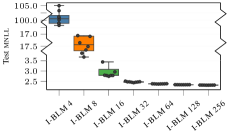
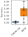
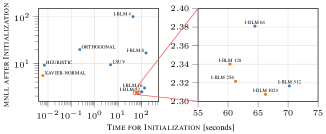
Previously we claimed that (i) small batches of data are sufficient to solve the Bayesian linear model and that (ii) our initialization does not suffer from timing complexity overhead. We now want to justify the aforementioned claims. We initialize a cnn (LeNet-5) on mnist with an increasing number of samples per batch; Figure Figure 3 shows how test log-likelihood is affected by this choice. Using the full training set leads to a better estimate of the posteriors and therefore of the likelihood. The mini-batch size affects also the heterogeneity of the posteriors, which vanishes when using the full training set. Nonetheless, we show that from 64/128 samples the improvement on the test mnll is only marginal. The same experiment is also repeated comparing test mnll after initialization between svi with i-blm and mcd (Figure Figure 3). Similar comments apply also for this case: i-blm allows the training to start from a lower negative log-likelihood. Finally, Figure 4 reports the test mnll after initialization as a function of the time required (orange points correspond to Pareto-optimal points). Before training, three out of four optimal initializers are i-blm.

5 Experimental Results

In this section, we compare different initialization algorithms for svi to prove the effectiveness of i-blm. We propose a number of competitors inspired from the literature developed for loss minimization in dnns and cnns. In the case of cnns, we also compare with Monte Carlo Dropout (mcd; Gal & Ghahramani (2016a)) and Natural Noisy Gradients (noisy-kfac; Zhang et al. (2018)), which respresent the state-of-the-art references for inference in Bayesian cnns. At layer $(l)$, given the fully-factorized variational distribution $q(W^{(l)})=\prod_{i,j}\mathcal{N}(w_{i,j}^{(l)}|\mu_{i,j},\sigma^{2}_{i,j})$, we initialize $\mu_{i,j}$ and $\sigma^{2}_{i,j}$ with the following methods.

Uninformative

The optimization of the posterior starts from the prior; therefore $q(W)=\prod_{i,j}\mathcal{N}(w_{i,j}|0,1)$. Note that this yields an initial kl divergence in the nelbo equal to zero.

Random Heuristic

An extension to commonly used heuristic with $\mu_{i,j}=0$ and $\sigma^{2}_{i,j}=\frac{1}{D_{\mathrm{in}}}$, with $D_{\mathrm{in}}$ the number of input features at layer $(l)$.

Xavier Normal

Originally proposed by Glorot & Bengio (2010), it samples all weights independently from a Gaussian distribution with zero mean and $\sigma^{2}=\frac{2}{D_{\mathrm{in}}+D_{\mathrm{out}}}$. This variance-based scaling avoids issues with vanishing or exploding gradients. In this case, it is straightforward to extend it to the case of svi; indeed, instead of sampling, we directly set $\mu_{i,j}=0$ and $\sigma^{2}_{i,j}=\frac{2}{D_{\mathrm{in}}+D_{\mathrm{out}}}$, knowing that the sampling is performed during the Monte Carlo estimate of the log-likelihood.

Orthogonal

Starting from an analysis of learning dynamics of dnns with linear activations, Saxe et al. (2013) propose an initialization scheme with orthonormal weight matrices. The idea is to decompose a Gaussian random matrix onto an orthonormal basis, and use the resulting orthogonal matrix. We adapt this method for svi by initializing the mean matrix with the orthogonal matrix and $\sigma^{2}_{i,j}=\frac{1}{D_{\mathrm{in}}}$. For our experiments, we use the implementation in pytorch (Paszke et al., 2017) provided by the Authors, which uses a QR-decomposition.

Figure 5: Progression of test rmse and test mnll with different initializations on a shallow architecture.

Layer-Sequential Unit-Variance (LSUV)

Starting from orthogonal initialization, Mishkin & Matas (2015) propose to perform a layer sequential variance scaling of the weight matrix. By implementing a data-driven greedy initialization, it generalizes the results to any nonlinear activation function and even to any type of layers that can impact the variance of the activations. We implement Layer-Sequential Unit-Variance (lsuv) for the means, while the variances are set to $\sigma^{2}_{i,j}=\frac{1}{D_{\mathrm{in}}}$.

5.1 Experiments

Throughout the experiments, we use adam optimizer (Kingma & Ba, 2015) with learning rate $10^{-3}$, batch size $64$, and $16$ Monte Carlo samples at training time and $128$ at test time. All experiments are run on a server equipped with two 16c/32t Intel Xeon CPU and four NVIDIA Tesla P100, with a maximum time budget of 24 hours (never reached). To better understand the effectiveness of different initialization, all learning curves are plotted w.r.t. training iteration rather than wall-clock time.

Regression with a shallow architecture

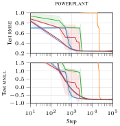
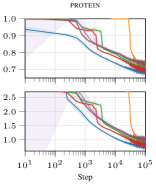
In this experiment we compare initialization methods for a shallow dnn architecture on two datasets. The architecture used in these experiments has one single hidden layer with $100$ hidden neurons and relu activations. We impose that the approximate posterior has fully factorized covariance. Figure 5 shows the learning curves on the powerplant ($n=9568$, $d=4$) and protein ($n=45730$, $d=9$) datasets, repeated over five different train/test splits. i-blm allows for a better initialization compared to the competitors, leading to a lower root mean square error (rmse) and lower mean negative log-likelihood (mnll) on the test for a given computational budget. We refer the reader to the supplementary material for a more detailed analysis of the results.

Regression with a deeper architecture

Figure 6: Progression of test rmse and test mnll with different initializations on a deep architecture.

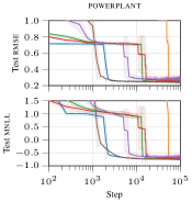
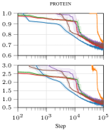
Similar considerations hold when increasing the depth of the model, keeping the same experimental setup. Figure 6 shows the progression of the rmse and mnll error metrics when using svi to infer parameters of a dnn with five hidden layers and $100$ hidden neurons per layer, and relu activations. Again, the proposed initialization allows svi to converge faster than when using other initializations.

Classification with a deep architecture

Figure 7: Progression of test error rate and test mnll with different initializations on classification problems.

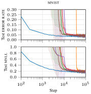
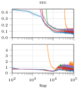
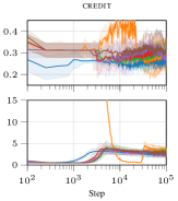
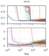
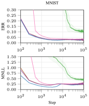
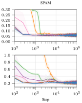
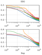
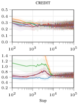
Using the same deep dnn architecture as in the last experiment (five hidden layers with $100$ neurons), we tested i-blm with classification problems on mnist ($n=70000$, $d=784$), eeg ($n=14980$, $d=14$), credit ($n=1000$, $d=24$) and spam ($n=4601$, $d=57$). Interestingly, with this architecture, some initialization strategies struggled to converge, e.g., uninformative on mnist and lsuv on eeg. The gains offered by i-blm achieves the most striking results on mnist. After less than $1000$ training steps (less than an epoch), it can already reach a test accuracy greater than $95\%$; other initalizations reach such performance much later during training. Even after $100$ epochs, svi inference initialized with i-blm provides on avarage an increase up to $14\%$ of accuracy at test time. Full results are reported in the supplementary material.

Experiments on CNNs

Figure 8: Progression of test error rate and test mnll for different initializations using LeNet-5 on mnist and cifar10. NB: uninformative, heuristic and xavier could never converged and therefore they are removed.

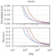
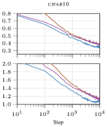
For this experiment, we implemented a Bayesian version of the original LeNet-5 architecture proposed by LeCun et al. (1998) with two convolutional layers of $6$ and $16$ filters, respectively and relu activations applied after all convolutional layers and fully-connected layers. We tested our framework on mnist and on cifar10. The only initialization strategies that achieve convergence are orthogonal and lsuv, along with i-blm; the other methods did not converge, meaning that they push the posterior back to the prior. Figure 8 reports the progression of error rate and mnll. For both mnist and cifar10, i-blm places the parameters where the network can consistently deliver better performance both in terms of error rate and mnll throughout the entire learning procedure.

Comparison with large scale models and non-Gaussian approximation

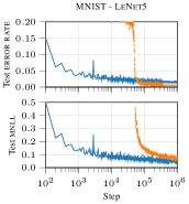
Monte Carlo Dropout (mcd; Gal & Ghahramani (2016b)) offers a simple and effective way to perform approximate Bayesian cnn inference, thanks to the connection that the Authors have established between dropout and variational inference. In this experiment, we aim to compare and discuss benefits and disadvantages of using a Gaussian posterior approximation with respect to the Bernoulli approximation that characterizes mcd. For a fair comparison, we implemented the same LeNet-5 architecture and the same learning procedure in Gal & Ghahramani (2016b). In particular, for mnist, the two convolutional layers have $20$ and $50$ filters, respectively. Dropout layers are placed after every convolutional and fully-connected layers with a dropout probability of $0.5$. To replicate the results in Gal & Ghahramani (2016b), we used the same learning rate policy $\texttt{base-lr}\times(1+\xi\times\texttt{iter})^{-p}$ with $\xi=0.0001$, $p=0.75$, $\texttt{base-lr}=0.01$ and weight decay of $0.0005$. Figure 9 shows the learning curves. Monte Carlo Dropout achieves state-of-art error rate but the form assumed by mcd for the posterior is reflected on an higher mnll compared to svi with a Gaussian posterior. Provided with a nontrivial initialization, Gaussian svi can better fit the model and deliver a better quantification of uncertainty.

Figure 9: Comparison between svi with Gaussian approximation and mcd on mnist and cifar10 with LeNet-5 and AlexNet.

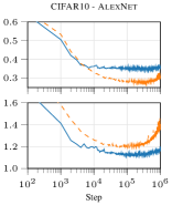
We report also error rate and mnll for svi with i-blm and mcd on AlexNet (Krizhevsky et al., 2012). The cnn is composed by a stack of five convolutional layers and three fully-connected layers for a total of more than $1$M parameters ($2$M for svi). In this experiment, we have experienced the situation in which, due to the overparameterization of the model, the nelbo is completely dominated by the kl divergence. Therefore, the prior has a large influence on the optimization, so we decided to follow the approach in Graves (2011), allowing for a phase of optimization of the variances of the prior over the parameters. The results are reported in Figure 9. Once again, we show that svi with i-blm provides a lower negative log-likelihood with respect to Bernoulli approximation in mcd.

Finally, we demonstrate that – provided with a sensible initialization – even simple factorized Gaussian posterior can achieve state-of-the-art performance on cifar10 with vgg16 , a large scale cnn (Simonyan & Zisserman, 2014). In this experiment, in addition to mcd, we compare with also with noisy-kfac, an approximation of matrix-variate Gaussian posterior using noisy natural gradients introduced by Zhang et al. (2018). In the case of Gaussian svi, to deal with over-parameterization, we implemented a policy where the kl term is gradually included in the nelbo (more details in the supplementary material). Results are shown in Figure 10 and in the adjacent Table. Gaussian svi delivers state-of-art test mnll while also providing a competitive test error rate.

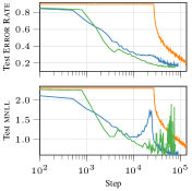
	mnll	error
i-blm	$\mathbf{0.6443}$	$\mathbf{0.1682}$
mcd	$0.8213$	$0.2147$
n-kfac	$0.7327$	$\mathbf{0.1506}$

[table]A table beside a figure

Figure 10: Comparison between Gaussian factorized svi, mcd and noisy-kfac on vgg16 with cifar10

Extended experimental evaluation

We refer the reader to the supplementary material for additional insights of i-blm compared with other initialization methods, analysis of out-of-sample uncertainty estimation, and tests of calibration properties of deep classifiers.

6 Conclusions

This work fills an important gap in the literature of Bayesian deep learning, that is how to effectively initialize variational parameters in svi. We proposed a novel way to do so, i-blm, which is based on an iterative layer-wise initialization based on Bayesian linear models. Through a series of experiments, including regression and classification with dnns and cnns, we demonstrated the ability of our approach to consistently initialize the optimization in a way that makes convergence faster than alternatives inspired from the state-of-the-art in loss minimization for deep learning.

Thanks to i-blm, it was possible to carry out an effective comparison with state-of-the-art methods to carry out approximate inference for dnns and cnns. This suggests a number of directions to investigate to improve on svi and Bayesian cnns. We found that the choice of the prior plays an important role in the behavior of the optimization, so we are investigating ways to define sensible priors for these models. Furthermore, we are looking into ways to extend our initialization strategy to more complex posterior distributions beyond Gaussian and to other deep models, such as Deep Gaussian Processes and Bayesian deep generative models.

Acknowledgements

MF gratefully acknowledges support from the AXA Research Fund.

Appendix A Full derivation of variational lower bound

$${{\textsc{kl}}}\left(q_{\theta}(\mathbf{W})||p(\mathbf{W}|X,Y)\right) =\mathbb{E}_{q_{\theta}}\left[\log\frac{q_{\theta}(\mathbf{W})}{p(\mathbf{W}|X,Y)}\right]=$$

$$=\mathbb{E}_{q_{\theta}}\left[\log q_{\theta}(\mathbf{W})-\log p(\mathbf{W}|X,Y)\right]=$$

$$=\mathbb{E}_{q_{\theta}}\left[-\log p(Y|X,\mathbf{W})\right]+\mathbb{E}_{q_{\theta}}\left[\log q_{\theta}(\mathbf{W})-\log p(\mathbf{W})\right]+\log p(Y|X)=$$

$$=\hbox{\pagecolor{white!50}$\displaystyle{\textsc{nll}}+{{\textsc{kl}}}\left(q_{\theta}(\mathbf{W})||p(\mathbf{W})\right)$}+\log p(Y|X)$$

Appendix B Bayesian linear regression

We express the likelihood and the prior on the parameters as follows:

$$p(Y|W,L)=\prod_{i}p(Y_{\cdot i}|XW_{\cdot i},L)=\prod_{i}\mathcal{N}(Y_{\cdot i}|XW_{\cdot i},L)$$

Denote by $X$ the $n\times d$ matrix containing $n$ input vectors $\mathbf{x}_{i}\in\mathbb{R}^{d}$, and let $Y$ be the set consisting of the corresponding multivariate labels $\mathbf{y}_{i}$. In Bayesian linear regression we introduce a set of latent variables that we compute as a linear combination of the input through a set of weights, and we express the likelihood and the prior on the parameters as follows:

$$p(Y|W,L)=\prod_{i}p(Y_{\cdot i}|XW_{\cdot i},\lambda)=\prod_{i}\mathcal{N}(Y_{\cdot i}|XW_{\cdot i},L)$$

and

$$p(W|\Lambda)=\prod_{i}p(W_{\cdot i})=\mathcal{N}(W_{\cdot i}|\mathbf{0},\Lambda)$$

The posterior of this model is:

$$p(W|Y,L)\propto\prod_{i}\mathcal{N}(Y_{\cdot i}|XW_{\cdot i},L)\mathcal{N}(W_{\cdot i}|\mathbf{0},\Lambda)$$

which implies that the posterior factorizes across the columns of $W$, with factors

$$p(W_{\cdot i}|Y,X,L,\Lambda)=\mathcal{N}(W_{\cdot i}|\Sigma_{i}X^{\top}L^{-1}Y_{\cdot i},\Sigma_{i})$$

with $\Sigma_{i}=(\Lambda^{-1}+X^{\top}L^{-1}X)^{-1}$. Similarly, the marginal likelihood factorizes as the product of the following factors

$$p(Y_{\cdot i}|X,L,\Lambda)=\mathcal{N}(Y_{\cdot i}|\mathbf{0},L+X\Lambda X^{\top})$$

Appendix C Heteroscedastic Bayesian linear regression

We can extend Bayesian linear regression to the heteroscedastic case where $L=\mathrm{diag}(\boldsymbol{\sigma}^{2})$ and $\Lambda=I$. These yield

$$p(W_{\cdot i}|Y,X,\boldsymbol{\sigma}^{2})=\mathcal{N}(W_{\cdot i}|\mu_{i},\Sigma_{i})\quad\mathrm{with}$$

$$\mu_{i}=\Sigma_{i}X^{\top}\mathrm{diag}(\boldsymbol{\sigma}^{-2})Y_{\cdot i}$$

$$\Sigma_{i}=(I+X^{\top}\mathrm{diag}(\boldsymbol{\sigma}^{-2})X)^{-1}$$

and

$$p(Y_{\cdot i}|X,\boldsymbol{\sigma}^{2})=\mathcal{N}(Y_{\cdot i}|\mathbf{0},\mathrm{diag}(\boldsymbol{\sigma}^{2})+XX^{\top})$$

The expression for the marginal likelihood is computationally unconvenient due to the need to deal with an $n\times n$ matrix. We can use Woodbury identities to express this calculation using $\Sigma_{i}$. In particular,

$$\log[p(Y_{\cdot i}|X,\boldsymbol{\sigma}^{2})]=-\frac{1}{2}\log\left|\mathrm{diag}(\boldsymbol{\sigma}^{2})+XX^{\top}\right|-\frac{1}{2}Y_{\cdot i}^{\top}\left(\mathrm{diag}(\boldsymbol{\sigma}^{2})+XX^{\top}\right)^{-1}Y_{\cdot i}+\mathrm{const.}$$

Using Woodbury identites, we can rewrite the algebraic operations as follows:

$$\log\left|\mathrm{diag}(\boldsymbol{\sigma}^{2})+XX^{\top}\right|=\log\left|\mathrm{diag}(\boldsymbol{\sigma}^{2})\right|+\log\left|I+\mathrm{diag}(\boldsymbol{\sigma}^{-2})XX^{\top}\right|=\sum_{j}\log\sigma^{2}_{j}+\log\left|I+X^{\top}\mathrm{diag}(\boldsymbol{\sigma}^{-2})X\right|$$

and

$$\left(\mathrm{diag}(\boldsymbol{\sigma}^{2})+XX^{\top}\right)^{-1}=\mathrm{diag}(\boldsymbol{\sigma}^{-2})-\mathrm{diag}(\boldsymbol{\sigma}^{-2})X\left(I+X^{\top}\mathrm{diag}(\boldsymbol{\sigma}^{-2})X\right)^{-1}X^{\top}\mathrm{diag}(\boldsymbol{\sigma}^{-2})$$

So, wrapping up, we ca express all quantities of interest as:

$$\Sigma_{i}^{-1}=I+X^{\top}\mathrm{diag}(\boldsymbol{\sigma}^{-2})X$$

$$\log[p(Y_{\cdot i}|X,\boldsymbol{\sigma}^{2})]=-\frac{1}{2}\left(\sum_{j}\log\sigma^{2}_{j}+\log\left|\Sigma_{i}^{-1}\right|\right)-\frac{1}{2}Y_{\cdot i}^{\top}\left(\mathrm{diag}(\boldsymbol{\sigma}^{-2})-\mathrm{diag}(\boldsymbol{\sigma}^{-2})X\Sigma_{i}X^{\top}\mathrm{diag}(\boldsymbol{\sigma}^{-2})\right)^{-1}Y_{\cdot i}+\mathrm{const.}$$

If we factorize $\Sigma_{i}^{-1}=QQ^{\top}$, we obtain:

$$\log[p(Y_{\cdot i}|X,\boldsymbol{\sigma}^{2})]=-\frac{1}{2}\left(\sum_{j}\log(\sigma^{2}_{j})+\sum_{k}2\log(Q_{kk})\right)-\frac{1}{2}Y_{\cdot i}^{\top}\tilde{Y}_{\cdot i}+\frac{1}{2}\tilde{Y}_{\cdot i}^{\top}XQ^{-\top}Q^{-1}X^{\top}\tilde{Y}_{\cdot i}+\mathrm{const.}$$

where $\tilde{Y}_{\cdot i}=\mathrm{diag}(\boldsymbol{\sigma}^{-2})Y_{\cdot i}$

Predictions follow from the same identities as before - looking at the predicted latent process, we have

$$p(f_{*i}|X,Y,\mathbf{x}_{*})=\int p(f_{*i}|W,\mathbf{x}_{*})p(W|X,Y)dW$$

We can again remove the dependence from the dimensions of $W$ that do not affect the prediction for the $i$th function as

$$p(f_{*i}|X,Y,\mathbf{x}_{*})=\int p(f_{*i}|W_{\cdot i},\mathbf{x}_{*})p(W_{\cdot i}|X,Y)dW$$

Now:

$$p(f_{*i}|W_{\cdot i},\mathbf{x}_{*})=\mathcal{N}(f_{*i}|\mathbf{x}_{*}^{\top}W_{\cdot i},0)\qquad\text{and}\qquad p(W_{\cdot i}|X,Y)=\mathcal{N}(W_{\cdot i}|\mu_{i},\Sigma_{i})$$

giving

$$p(f_{*i}|X,Y,\mathbf{x}_{*})=\mathcal{N}(f_{*i}|\mathbf{x}_{*}^{\top}\mu_{i},\mathbf{x}_{*}^{\top}\Sigma_{i}\mathbf{x}_{*})$$

Appendix D Full derivation of fully factorized Gaussian posterior approximation to Bayesian linear regression posterior

For simplicity of notation, let $\mathbf{w}$ be the parameters of interest in Bayesian linear regression for a given output $\mathbf{y}=Y_{\cdot i}$. We can formulate the problem of obtaining the best approximate factorized posterior of a Bayeian linear model as a minimization of the Kullback-Leibler divergence between $q(\mathbf{w})=\mathcal{N}(\mathbf{w}|\mathbf{m},\mathrm{diag}(\mathbf{s}^{2}))$ and the actual posterior $p(\mathbf{w}|X,\mathbf{y})$. The expression of the KL divergence between multivariate Gaussians $p_{0}=\mathcal{N}(W|\boldsymbol{\mu}_{0},\Sigma_{0})$ and $p_{1}=\mathcal{N}(W|\boldsymbol{\mu}_{1},\Sigma_{1})$ is as follows:

$$\mathrm{KL}[p_{0}||p_{1}]=\frac{1}{2}\mathrm{Tr}(\Sigma_{1}^{-1}\Sigma_{0})+\frac{1}{2}(\boldsymbol{\mu}_{1}-\boldsymbol{\mu}_{0})^{\top}\Sigma_{1}^{-1}(\boldsymbol{\mu}_{1}-\boldsymbol{\mu}_{0})-\frac{D}{2}+\frac{1}{2}\log\left(\frac{\mathrm{det}\Sigma_{1}}{\mathrm{det}\Sigma_{0}}\right)$$

The KL divergence is not symmetric, so the order in which we take this matters. In case we consider $\mathrm{KL}[p(\mathbf{w}|X,\mathbf{y})||q(\mathbf{w})]$, the expression becomes:

$$\mathrm{KL}[p(\mathbf{w}|X,\mathbf{y})||q(\mathbf{w})]=\frac{1}{2}\mathrm{Tr}(\mathrm{diag}(\mathbf{s}^{2})^{-1}\Sigma)+\frac{1}{2}(\mathbf{m}-\boldsymbol{\mu})^{\top}\mathrm{diag}(\mathbf{s}^{2})^{-1}(\mathbf{m}-\boldsymbol{\mu})-\frac{D}{2}+\frac{1}{2}\log\left(\frac{\prod_{i}s_{i}^{2}}{\mathrm{det}\Sigma}\right)$$

It is a simple matter to show that the optimal mean $\mathbf{m}$ is $\boldsymbol{\mu}$ as $\mathbf{m}$ appears only in the quadratic form which is clearly minimized when $\mathbf{m}=\boldsymbol{\mu}$. For the variances $\mathbf{s}^{2}$, we need to take the derivative of the KL divergence and set it to zero:

$$\frac{\partial\mathrm{KL}[p(\mathbf{w}|X,\mathbf{y})||q(\mathbf{w})]}{\partial s^{2}_{i}}=\frac{1}{2}\frac{\partial\mathrm{Tr}(\mathrm{diag}(\mathbf{s}^{2})^{-1}\Sigma)}{\partial s_{i}^{2}}+\frac{1}{2}\frac{\partial\sum_{i}\log{s_{i}^{2}}}{\partial s_{i}^{2}}=0$$

Rewriting the trace term as the sum of the Hadamrd product of the matrices in the product $\sum_{ij}(\mathrm{diag}(\mathbf{s}^{2})^{-1}\odot\Sigma)_{ij}=\sum_{i}\Sigma_{ii}/s_{i}^{2}$, this yields

$$\frac{\partial\mathrm{KL}[p(\mathbf{w}|X,\mathbf{y})||q(\mathbf{w})]}{\partial s^{2}_{i}}=\frac{1}{2}\frac{\partial\Sigma_{ii}/s_{i}^{2})}{\partial s_{i}^{2}}+\frac{1}{2}\frac{\partial\log{s_{i}^{2}}}{\partial s_{i}^{2}}=0$$

This results in $s_{i}^{2}=\Sigma_{ii}$, which is the simplest way to approximate the correlated posterior over $\mathbf{w}$ but it is going to inflate the variance in case of strong correlations.

In case we consider $\mathrm{KL}[q(\mathbf{w})||p(\mathbf{w}|X,\mathbf{y})]$, the expression of the KL becomes:

$$\mathrm{KL}[q(\mathbf{w})||p(\mathbf{w}|X,\mathbf{y})]=\frac{1}{2}\mathrm{Tr}(\Sigma^{-1}\mathrm{diag}(\mathbf{s}^{2}))+\frac{1}{2}(\mathbf{m}-\boldsymbol{\mu})^{\top}\Sigma^{-1}(\mathbf{m}-\boldsymbol{\mu})-\frac{D}{2}+\frac{1}{2}\log\left(\frac{\mathrm{det}\Sigma}{\prod_{i}s_{i}^{2}}\right)$$

Again, the optimal mean $\mathbf{m}$ is $\boldsymbol{\mu}$. For the variances $\mathbf{s}^{2}$, we need to take the derivative of the KL divergence and set it to zero:

$$\frac{\partial\mathrm{KL}[q(\mathbf{w})||p(\mathbf{w}|X,\mathbf{y})]}{\partial s^{2}_{i}}=\frac{1}{2}\frac{\partial\mathrm{Tr}(\Sigma^{-1}\mathrm{diag}(\mathbf{s}^{2}))}{\partial s_{i}^{2}}-\frac{1}{2}\frac{\partial\sum_{i}\log{s_{i}^{2}}}{\partial s_{i}^{2}}=0$$

Rewriting the trace term as the sum of the Hadamrd product of the matrices in the product $\sum_{ij}(\Sigma^{-1}\odot\mathrm{diag}(\mathbf{s}^{2}))_{ij}=\sum_{i}s_{i}^{2}\Sigma^{-1}_{ii}$, this yields

$$\frac{\partial\mathrm{KL}[q(\mathbf{w})||p(\mathbf{w}|X,\mathbf{y})]}{\partial s^{2}_{i}}=\frac{1}{2}\frac{\partial s_{i}^{2}\Sigma^{-1}_{ii})}{\partial s_{i}^{2}}-\frac{1}{2}\frac{\partial\log{s_{i}^{2}}}{\partial s_{i}^{2}}=0$$

This results in $(s_{i}^{2})^{-1}=\Sigma^{-1}_{ii}$. This approximation has the opposite effect of underestimating the variance for each variable.

Appendix E Extended results

E.1 Toy example

Figure 11: Predictions after initialization using our proposal and all the other competitive methods.

With this simple example we want once more illustrate how i-blm works and how it can speed up the convergence of svi. We set up a regression problem considering the function $f(x)=\sin(x)+\sin(x/2)+\sin(x/3)-\sin(x/4)$ corrupted by noise $\varepsilon\sim\mathcal{N}(0,\exp(-2))$, with $x$ sampled uniformly in the interval $[-10,10]$. Figure 11 reports the output of a $4$-layer dnn after different initializations. The figure shows that i-blm obtains a sensible initialization compared to the competitors.

E.2 Regression with shallow architecture

test rmse
	i-blm	uninformative	heuristic	xavier	orthogonal	lsuv
powerplant	$\mathbf{0.2427\pm 0.006}$	$0.2452\pm 0.007$	$0.2436\pm 0.008$	$0.2427\pm 0.008$	$0.2439\pm 0.008$	$0.2438\pm 0.007$
protein	$\mathbf{0.6831\pm 0.004}$	$0.7135\pm 0.008$	$0.7020\pm 0.009$	$0.6952\pm 0.011$	$0.7315\pm 0.016$	$0.7356\pm 0.006$
test mnll
	i-blm	uninformative	heuristic	xavier	orthogonal	lsuv
powerplant	$\mathbf{-0.7647\pm 0.012}$	$-0.7607\pm 0.013$	$-0.7622\pm 0.014$	$-0.7641\pm 0.013$	$-0.7623\pm 0.013$	$-0.7623\pm 0.012$
protein	$\mathbf{0.7510\pm 0.021}$	$0.8980\pm 0.040$	$0.8376\pm 0.046$	$0.8047\pm 0.055$	$0.9878\pm 0.083$	$1.0081\pm 0.033$

E.3 Regression with deep architecture

test rmse
	i-blm	uninformative	heuristic	xavier	orthogonal	lsuv
powerplant	$0.2472\pm 0.003$	$0.2476\pm 0.005$	$\mathbf{0.2462\pm 0.005}$	$0.2658\pm 0.030$	$0.2467\pm 0.005$	$0.2774\pm 0.026$
protein	$\mathbf{0.6683\pm 0.007}$	$0.7170\pm 0.013$	$0.6899\pm 0.011$	$0.6821\pm 0.007$	$0.6982\pm 0.014$	$0.7033\pm 0.011$
test mnll
	i-blm	uninformative	heuristic	xavier	orthogonal	lsuv
powerplant	$\mathbf{-0.7455\pm 0.008}$	$-0.7420\pm 0.008$	$-0.7455\pm 0.009$	$-0.7007\pm 0.070$	$-0.7450\pm 0.010$	$-0.6677\pm 0.065$
protein	$\mathbf{0.6922\pm 0.035}$	$0.9326\pm 0.066$	$0.7884\pm 0.055$	$0.7540\pm 0.033$	$0.8280\pm 0.072$	$0.8587\pm 0.040$

E.4 Classification with shallow architecture

Figure 12: Progression of test error rate and test mnll over training iterations for different initialization strategies on four classification datasets.

test error rate
	i-blm	uninformative	heuristic	xavier	orthogonal	lsuv
spam	$\mathbf{0.0594\pm 0.013}$	$0.0620\pm 0.008$	$0.0624\pm 0.011$	$0.0620\pm 0.012$	$0.0611\pm 0.012$	$0.0598\pm 0.014$
eeg	$\mathbf{0.1855\pm 0.015}$	$0.1929\pm 0.009$	$0.2221\pm 0.009$	$0.2137\pm 0.008$	$0.2335\pm 0.007$	NC
credit	$0.2680\pm 0.027$	$0.2679\pm 0.044$	$\mathbf{0.2480\pm 0.071}$	$0.2519\pm 0.033$	$0.2539\pm 0.032$	$0.2580\pm 0.050$
mnist	$\mathbf{0.0253\pm 7\mathrm{e}{-4}}$	NC	$0.1046\pm 0.014$	$0.0315\pm 0.001$	$0.0275\pm 0.001$	$0.0291\pm 0.002$
test mnll
	i-blm	uninformative	heuristic	xavier	orthogonal	lsuv
spam	$0.229\pm 0.034$	$\mathbf{0.213\pm 0.030}$	$0.228\pm 0.043$	$0.228\pm 0.048$	$0.225\pm 0.053$	$0.228\pm 0.050$
eeg	$\mathbf{0.4218\pm 0.020}$	$0.4668\pm 0.008$	$0.4411\pm 0.006$	$0.4866\pm 0.010$	$0.4728\pm 0.010$	NC
credit	$0.6759\pm 0.084$	$\mathbf{0.6597\pm 0.101}$	$0.6605\pm 0.111$	$0.6616\pm 0.105$	$0.6662\pm 0.076$	$0.6739\pm 0.069$
mnist	$0.2655\pm 0.015$	NC	$0.4497\pm 0.039$	$0.2724\pm 0.020$	$\mathbf{0.2643\pm 0.017}$	$0.2744\pm 0.014$

E.5 Classification with deep architecture

test error rate
	i-blm	uninformative	heuristic	xavier	orthogonal	lsuv
mnist	$\mathbf{0.0356\pm 0.003}$	$0.0390\pm 0.003$	$0.0400\pm 0.003$	$0.0411\pm 0.002$	$0.0396\pm 0.002$	$0.0373\pm 0.001$
eeg	$\mathbf{0.0673\pm 0.008}$	$0.1283\pm 0.009$	$0.1119\pm 0.008$	$0.0894\pm 0.003$	$0.1216\pm 0.002$	NC
credit	$\mathbf{0.2700\pm 0.024}$	$0.2975\pm 0.059$	$0.2824\pm 0.058$	$0.2833\pm 0.022$	$0.3145\pm 0.051$	$0.2758\pm 0.022$
spam	$0.0566\pm 0.021$	$0.0611\pm 0.008$	$0.0585\pm 0.017$	$0.0534\pm 0.018$	$\mathbf{0.0514\pm 0.013}$	$0.0611\pm 0.013$
test mnll
	i-blm	uninformative	heuristic	xavier	orthogonal	lsuv
mnist	$\mathbf{0.1692\pm 0.007}$	$0.1847\pm 0.002$	$0.1799\pm 0.009$	$0.1912\pm 0.011$	$0.1822\pm 0.005$	$0.1723\pm 0.005$
eeg	$\mathbf{0.4222\pm 0.054}$	$1.2515\pm 0.352$	$0.8136\pm 0.123$	$0.6273\pm 0.130$	$0.9366\pm 0.097$	NC
credit	$2.6555\pm 0.521$	$3.2836\pm 0.704$	$3.1268\pm 0.678$	$2.7015\pm 0.665$	$2.6482\pm 0.231$	$\mathbf{2.5422\pm 0.236}$
spam	$\mathbf{0.7021\pm 0.218}$	$1.1098\pm 0.271$	$1.0458\pm 0.517$	$1.0682\pm 0.347$	$0.8176\pm 0.337$	$1.1682\pm 0.486$

E.6 Convolutional neural networks

test error rate
	i-blm	uninformative	heuristic	xavier	orthogonal	lsuv
mnist	$\mathbf{0.0087}$	NC	NC	NC	$0.0098$	$0.0113$
cifar10	$\mathbf{0.3499}$	NC	NC	NC	$0.3784$	$0.3846$
test mnll
	i-blm	uninformative	heuristic	xavier	orthogonal	lsuv
mnist	$\mathbf{0.0345}$	NC	NC	NC	$0.0377$	$0.0421$
cifar10	$\mathbf{1.0683}$	NC	NC	NC	$1.1270$	$1.1428$

E.7 Uncertainty estimation

Figure 13: Entropy distribution while testing on mnist and not-mnist (higher average entropy on not-mnist means better uncertainty estimation).

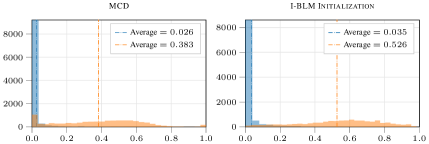
One of the advantages of Bayesian inference is the possibility to reason about uncertainty. With this experiment, we aim to demonstrate that svi with a Gaussian approximate posterior is competitive with mcd in capturing uncertainty in predictions. To show this, we focus on a cnn with the LeNet-5 architecture. We run mcd and svi with a Gaussian approximate posterior with the proposed initialization on mnist. At test time, we carry out predictions on both mnist and not-mnist; the latter is a dataset equivalent to mnist in input dimensions ($1\times 28\times 28$) and number of classes, but it represents letters rather than numbers. This experimental setup is often used to check that the entropy of the predictions on not-mnist are actually higher than the entropy of the predictions on mnist. We report the entropy of the prediction on mnist and not-mnist in Figure 13. mcd and svi behave similarly on mnist, but on not-mnist the the histogram of the entropy indicates that svi yields a slightly higher uncertainty compared to mcd.

E.8 Calibration

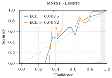
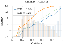
Calibration of uncertainty is an important performance metric that one should take into account for comparing classification models (Flach, 2016; Guo et al., 2017). Reliability Diagrams and the Expected Calibration Error are standard methods to empirically estimate the calibration uncertainty. Reliability Diagrams are a visualization tool where sample accuracy is plotted as function of confidence (DeGroot & Fienberg, 1983; Niculescu-Mizil & Caruana, 2005). For a perfectly calibrated model, the diagram follows the identity function. Expected Calibration Error (or ece) represents a summary statistic of the calibration (Naeini et al., 2015). Figure 14 shows the reliability diagrams and the ece for LeNet-5 trained on mnist and for AlexNet trained on cifar10. Even tough they show similar properties on mnist, with AlexNet on cifar10, svi initialized with i-blm improves the calibration of uncertainty up to $3.5$ times over mcd.

Figure 14: Comparison of reliability diagrams and ece between i-blm and mcd on mnist (left) and cifar10 (right).

E.9 kl regularization policy for Gaussian svi

The kl regularization term in the variational objective severely penalizes training of over-parameterized model. With a sensible initialization of this kind of model, the approximate posterior is drastically different from a spherical Gaussian prior and the variational objective is majorly dominated by the regularization term rather than the reconstruction likelihood. To deal with such issue, we propose and implement a simple policy to gradually include the kl term in the nelbo. Given the generic expression for the nelbo, we modify the lower bound as follow:

$${\textsc{nelbo}}={\textsc{nll}}+\lambda{{\textsc{kl}}}\left(q_{\boldsymbol{\theta}}(\mathbf{W})||p(\mathbf{W})\right)\quad\text{where}\quad\lambda=\gamma\left(1+\exp(-\alpha(\text{iter}-\beta))\right)^{-1}\,,$$

This way, we start the optimization of the nelbo with low regularization, and progressively increase it throughout the optimization. For the experiment on vgg16, we used $\alpha=2\cdot 10^{-3}$, $\beta=2.5\cdot 10^{4}$ and $\gamma=10^{-1}$.

References

- Baldi & Hornik (1989) Baldi, P. and Hornik, K. Neural networks and principal component analysis: Learning from examples without local minima. Neural Networks, 2(1):53–58, 1989. ISSN 08936080.
- Bengio et al. (2006) Bengio, Y., Lamblin, P., Popovici, D., and Larochelle, H. Greedy layer-wise training of deep networks. In Adv. in Neural Inf. Proc. Syst. 19, pp. 153–160, 2006.
- Bishop (2006) Bishop, C. M. Pattern recognition and machine learning. Springer, 1st ed. 2006. corr. 2nd printing 2011 edition, August 2006. ISBN 0387310738.
- Buchholz et al. (2018) Buchholz, A., Wenzel, F., and Mandt, S. Quasi-Monte Carlo variational inference. In Proceedings of the 35th International Conference on Machine Learning, volume 80 of Proceedings of Machine Learning Research, pp. 668–677, Stockholm, Sweden, 10–15 Jul 2018. PMLR.
- DeGroot & Fienberg (1983) DeGroot, M. H. and Fienberg, S. E. The comparison and evaluation of forecasters. Journal of the Royal Statistical Society. Series D (The Statistician), 32(1/2):12–22, 1983. ISSN 00390526, 14679884.
- Duchi et al. (2011) Duchi, J., Hazan, E., and Singer, Y. Adaptive Subgradient Methods for Online Learning and Stochastic Optimization. Journal of Machine Learning Research, 12:2121–2159, July 2011.
- Dziugaite & Roy (2017) Dziugaite, G. K. and Roy, D. M. Computing Nonvacuous Generalization Bounds for Deep (Stochastic) Neural Networks with Many More Parameters than Training Data, October 2017. arXiv:1703.11008.
- Erhan et al. (2010) Erhan, D., Courville, A., and Vincent, P. Why Does Unsupervised Pre-training Help Deep Learning? Journal of Machine Learning Research, 11:625–660, 2010. ISSN 15324435.
- Flach (2016) Flach, P. A. Classifier Calibration. In Sammut, C. and Webb, G. I. (eds.), Encyclopedia of Machine Learning and Data Mining, pp. 1–8. Springer US, Boston, MA, 2016.
- Gal & Ghahramani (2016a) Gal, Y. and Ghahramani, Z. Dropout As a Bayesian Approximation: Representing Model Uncertainty in Deep Learning. In Proceedings of the 33rd International Conference on International Conference on Machine Learning - Volume 48, ICML’16, pp. 1050–1059. JMLR.org, 2016a.
- Gal & Ghahramani (2016b) Gal, Y. and Ghahramani, Z. Bayesian Convolutional Neural Networks with Bernoulli Approximate Variational Inference, January 2016b. arXiv:1506.02158.
- Gal et al. (2017) Gal, Y., Hron, J., and Kendall, A. Concrete Dropout. In Guyon, I., Luxburg, U. V., Bengio, S., Wallach, H., Fergus, R., Vishwanathan, S., and Garnett, R. (eds.), Advances in Neural Information Processing Systems 30, pp. 3581–3590. Curran Associates, Inc., 2017.
- Ghahramani (2015) Ghahramani, Z. Probabilistic machine learning and artificial intelligence. Nature, 521(7553):452–459, May 2015. ISSN 0028-0836.
- Glorot & Bengio (2010) Glorot, X. and Bengio, Y. Understanding the difficulty of training deep feedforward neural networks. PMLR, 9:249–256, 2010. ISSN 15324435.
- Graves (2011) Graves, A. Practical Variational Inference for Neural Networks. In Shawe-Taylor, J., Zemel, R. S., Bartlett, P. L., Pereira, F., and Weinberger, K. Q. (eds.), Advances in Neural Information Processing Systems 24, pp. 2348–2356. Curran Associates, Inc., 2011.
- Guo et al. (2017) Guo, C., Pleiss, G., Sun, Y., and Weinberger, K. Q. On Calibration of Modern Neural Networks. In Precup, D. and Teh, Y. W. (eds.), Proceedings of the 34th International Conference on Machine Learning, volume 70 of Proceedings of Machine Learning Research, pp. 1321–1330, International Convention Centre, Sydney, Australia, August 2017. PMLR.
- Ha et al. (2016) Ha, D., Dai, A. M., and Le, Q. V. HyperNetworks, 2016. arXiv:1609.09106.
- He et al. (2016) He, K., Zhang, X., Ren, S., and Sun, J. Deep Residual Learning for Image Recognition. In 2016 IEEE Conference on Computer Vision and Pattern Recognition, CVPR 2016, Las Vegas, NV, USA, June 27-30, 2016, pp. 770–778, 2016.
- Hinton & van Camp (1993) Hinton, G. E. and van Camp, D. Keeping the neural networks simple by minimizing the description length of the weights. In Proceedings of the sixth annual conference on Computational learning theory - COLT ’93, 1993. ISBN 0897916115.
- Huang et al. (2018) Huang, C.-W., Krueger, D., Lacoste, A., and Courville, A. Neural autoregressive flows. In Proceedings of the 35th International Conference on Machine Learning, volume 80 of Proceedings of Machine Learning Research, pp. 2078–2087, Stockholm, Sweden, 10–15 Jul 2018. PMLR.
- Jia (2014) Jia, Y. Learning Semantic Image Representations at a Large Scale. PhD thesis, Berkeley, California, 2014.
- Jordan et al. (1999) Jordan, M. I., Ghahramani, Z., Jaakkola, T. S., and Saul, L. K. An Introduction to Variational Methods for Graphical Models. Machine Learning, 37(2):183–233, November 1999.
- Kendall & Gal (2017) Kendall, A. and Gal, Y. What Uncertainties Do We Need in Bayesian Deep Learning for Computer Vision? In Guyon, I., Luxburg, U. V., Bengio, S., Wallach, H., Fergus, R., Vishwanathan, S., and Garnett, R. (eds.), Advances in Neural Information Processing Systems 30, pp. 5574–5584. Curran Associates, Inc., 2017.
- Kingma & Ba (2015) Kingma, D. P. and Ba, J. Adam: A Method for Stochastic Optimization. In International Conference on Learning Representations (ICLR), San Diego, may 2015.
- Kingma & Welling (2014) Kingma, D. P. and Welling, M. Auto-Encoding Variational Bayes. In Proceedings of the Second International Conference on Learning Representations (ICLR 2014), April 2014.
- Kingma et al. (2015) Kingma, D. P., Salimans, T., and Welling, M. Variational dropout and the local reparameterization trick. In Advances in Neural Information Processing Systems 28, pp. 2575–2583. 2015.
- Kingma et al. (2016) Kingma, D. P., Salimans, T., Jozefowicz, R., Chen, X., Sutskever, I., and Welling, M. Improving Variational Inference with Inverse Autoregressive Flow. In Advances in Neural Information Processing Systems 29, pp. 4743–4751. 2016.
- Krishnan et al. (2018) Krishnan, R., Liang, D., and Hoffman, M. On the challenges of learning with inference networks on sparse, high-dimensional data. In Storkey, A. and Perez-Cruz, F. (eds.), Proceedings of the Twenty-First International Conference on Artificial Intelligence and Statistics, volume 84 of Proceedings of Machine Learning Research, pp. 143–151, Playa Blanca, Lanzarote, Canary Islands, 09–11 Apr 2018. PMLR.
- Krizhevsky et al. (2012) Krizhevsky, A., Sutskever, I., and Hinton, G. E. ImageNet Classification with Deep Convolutional Neural Networks. Advances In Neural Information Processing Systems, 2012. ISSN 10495258.
- Kullback (1959) Kullback, S. Information Theory and Statistics. 1959. ISBN 0780327616.
- Lakshminarayanan et al. (2017) Lakshminarayanan, B., Pritzel, A., and Blundell, C. Simple and Scalable Predictive Uncertainty Estimation using Deep Ensembles. In Guyon, I., Luxburg, U. V., Bengio, S., Wallach, H., Fergus, R., Vishwanathan, S., and Garnett, R. (eds.), Advances in Neural Information Processing Systems 30, pp. 6402–6413. Curran Associates, Inc., 2017.
- LeCun (1998) LeCun, Y. Efficient backprop. Neural networks: tricks of the trade, 53(9):1689–1699, 1998. ISSN 1098-6596.
- LeCun et al. (1998) LeCun, Y., Bottou, L., Bengio, Y., and Haffner, P. Gradient-based learning applied to document recognition. Proceedings of the IEEE, 86(11):2278–2323, 1998. ISSN 00189219.
- LeCun et al. (2015) LeCun, Y., Bengio, Y., and Hinton, G. Deep learning. Nature, 521(7553):436–444, 2015.
- Liu & Wang (2016) Liu, Q. and Wang, D. Stein Variational Gradient Descent: A General Purpose Bayesian Inference Algorithm. In Advances in Neural Information Processing Systems 29, pp. 2378–2386. 2016.
- Louizos & Welling (2016a) Louizos, C. and Welling, M. Structured and efficient variational deep learning with matrix gaussian posteriors. In Balcan, M. F. and Weinberger, K. Q. (eds.), Proceedings of The 33rd International Conference on Machine Learning, volume 48 of Proceedings of Machine Learning Research, pp. 1708–1716, New York, New York, USA, 20–22 Jun 2016a. PMLR.
- Louizos & Welling (2016b) Louizos, C. and Welling, M. Structured and efficient variational deep learning with matrix gaussian posteriors. In Balcan, M. F. and Weinberger, K. Q. (eds.), Proceedings of The 33rd International Conference on Machine Learning, volume 48 of Proceedings of Machine Learning Research, pp. 1708–1716, New York, New York, USA, 20–22 Jun 2016b. PMLR.
- Louizos & Welling (2017) Louizos, C. and Welling, M. Multiplicative Normalizing Flows for Variational Bayesian Neural Networks. In Proceedings of the 34th International Conference on Machine Learning, volume 70 of Proceedings of Machine Learning Research, pp. 2218–2227, Sydney, Australia, 06–11 Aug 2017. PMLR.
- MacKay (1992) MacKay, D. J. C. A Practical Bayesian Framework for Backpropagation Networks. Neural Computation, 4(3):448–472, may 1992. ISSN 0899-7667.
- Milios et al. (2018) Milios, D., Camoriano, R., Michiardi, P., Rosasco, L., and Filippone, M. Dirichlet-based Gaussian Processes for Large-scale Calibrated Classification. In Advances in Neural Information Processing System 31 (to appear), may 2018.
- Miller et al. (2017) Miller, A. C., Foti, N. J., and Adams, R. P. Variational Boosting: Iteratively Refining Posterior Approximations. In Proceedings of the 34th International Conference on Machine Learning, volume 70 of Proceedings of Machine Learning Research, pp. 2420–2429, Sydney, Australia, 06–11 Aug 2017. PMLR.
- Mishkin & Matas (2015) Mishkin, D. and Matas, J. All you need is a good init. arXiv preprint arXiv:1511.06422, nov 2015. ISSN 08981221.
- Naeini et al. (2015) Naeini, M. P., Cooper, G. F., and Hauskrecht, M. Obtaining well calibrated probabilities using Bayesian binning. In AAAI, pp. 2901–2907. AAAI Press, 2015.
- Neal (1997) Neal, R. M. Bayesian Learning for Neural Networks. Journal of the American Statistical Association, 1997. ISSN 01621459.
- Niculescu-Mizil & Caruana (2005) Niculescu-Mizil, A. and Caruana, R. Predicting Good Probabilities with Supervised Learning. In Proceedings of the 22Nd International Conference on Machine Learning, ICML ’05, pp. 625–632, New York, NY, USA, 2005. ACM.
- Paszke et al. (2017) Paszke, A., Chanan, G., Lin, Z., Gross, S., Yang, E., Antiga, L., and Devito, Z. Automatic differentiation in PyTorch. Advances in Neural Information Processing Systems 30, 2017.
- Ranganath et al. (2015) Ranganath, R., Tang, L., Charlin, L., and Blei, D. M. Deep Exponential Families. In Proceedings of the Eighteenth International Conference on Artificial Intelligence and Statistics, AISTATS 2015, San Diego, California, USA, May 9-12, 2015, 2015.
- Rezende & Mohamed (2015) Rezende, D. and Mohamed, S. Variational Inference with Normalizing Flows. In Proceedings of the 32nd International Conference on Machine Learning, volume 37 of Proceedings of Machine Learning Research, pp. 1530–1538, Lille, France, 07–09 Jul 2015. PMLR.
- Rezende et al. (2014) Rezende, D. J., Mohamed, S., and Wierstra, D. Stochastic Backpropagation and Approximate Inference in Deep Generative Models. In Jebara, T. and Xing, E. P. (eds.), Proceedings of the 31st International Conference on Machine Learning (ICML-14), pp. 1278–1286. JMLR Workshop and Conference Proceedings, 2014.
- Rumelhart et al. (1986) Rumelhart, D. E., Hinton, G. E., and Williams, R. J. Learning representations by back-propagating errors. Nature, 323(6088):533–536, oct 1986. ISSN 0028-0836.
- Saxe et al. (2013) Saxe, A. M., McClelland, J. L., and Ganguli, S. Exact solutions to the nonlinear dynamics of learning in deep linear neural networks. CoRR, abs/1312.6:1–22, dec 2013.
- Simonyan & Zisserman (2014) Simonyan, K. and Zisserman, A. Very Deep Convolutional Networks for Large-Scale Image Recognition. CoRR, abs/1409.1556, 2014.
- Srivastava et al. (2014) Srivastava, N., Hinton, G., Krizhevsky, A., Sutskever, I., and Salakhutdinov, R. Dropout: A Simple Way to Prevent Neural Networks from Overfitting. Journal of Machine Learning Research, 15(1):1929–1958, January 2014.
- Sutskever et al. (2013) Sutskever, I., Martens, J., Dahl, G., and Hinton, G. E. On the importance of initialization and momentum in deep learning. Proceedings of Machine Learning Research, (2010):1139–1147, feb 2013. ISSN 15206149.
- Zeiler (2012) Zeiler, M. D. ADADELTA: An Adaptive Learning Rate Method. arXiv, pp. 6, dec 2012. ISSN 09252312.
- Zhang et al. (2018) Zhang, G., Sun, S., Duvenaud, D., and Grosse, R. Noisy natural gradient as variational inference. In Dy, J. and Krause, A. (eds.), Proceedings of the 35th International Conference on Machine Learning, volume 80 of Proceedings of Machine Learning Research, pp. 5852–5861, Stockholmsmässan, Stockholm Sweden, 10–15 Jul 2018. PMLR.