Modeling and In-Database Management of
Relational, Data-Aware Processes (Extended Version)

Abstract

During the last two decades, it has been increasingly acknowledged that the engineering of information systems usually requires a huge effort in integrating master data and business processes. This has led to a plethora of proposals, both from academia and the industry. However, such approaches typically come with ad-hoc abstractions to represent and interact with the data component. This has a twofold disadvantage. On the one hand, they cannot be used to effortlessly enrich an existing relational database with dynamics. On the other hand, they generally do not allow for integrated modelling, verification, and enactment. We attack these two challenges by proposing a declarative approach, fully grounded in SQL, that supports the agile modelling of relational data-aware processes directly on top of relational databases. We show how this approach can be automatically translated into a concrete procedural SQL dialect, executable directly inside any relational database engine. The translation exploits an in-database representation of process states that, in turn, is used to handle, at once, process enactment with or without logging of the executed instances, as well as process verification. The approach has been implemented in a working prototype.

1 Introduction

During the last two decades, increasing attention has been given to the challenging problem, still persisting in modern organizations [19], of resolving the dichotomy between business process management and master data management [9, 18, 3]. Devising integrated models and corresponding enactment platforms for processes and data is now acknowledged as a necessary step to tame a number of conceptual and enterprise engineering issues, which cannot be tackled by implementation solutions applied at the level of the enterprise IT infrastructure.

This triggered a flourishing line of research on concrete languages for data-aware processes, and on the development of tools to model and enact such processes. The main unifying theme for such approaches is a shift from standard activity-centric business process meta-models, to a data-centric paradigm that focuses first on the elicitation of business entities, and then on their behavioral aspects. Notable approaches in this line are artifact-centric [9], object-centric [11] and data-centric models [21]. In parallel to these new modeling paradigms, also BPMS based on standard, activity-centric approaches a là BPMN, have increasingly incorporated data-related aspects in their tool support. Many modern BPM platforms provide (typically proprietary) data models, ad-hoc user interfaces to indicate how process tasks induce data updates, and query languages to express decisions based on data. While this approach has the main advantage of hiding the complexity of the underlying relational database (DB) from the modeler, it comes with two critical shortcomings. First, it makes it difficult to conceptually understand the overall process in terms of general, tool-agnostic principles, and to redeploy the same process in a different BPMS. This is witnessed by a number of ongoing proposals that explicitly bring forward complex mappings for model-to-model transformation (see, e.g., [26, 10]).

Second, this approach cannot be readily applied in the recurrent case where the process needs to be integrated with existing DB tables. In fact, updating an underlying DB through a more abstract data model is an extremely challenging problem that cannot be solved in general, and that is reminiscent to the long-standing, well-known view update problem in the database literature [8]. This is often handled by doing the strong assumption that the entire DB schema over which the process (indirectly) operates can be fully generated from the adopted data model, or connected in a lossless way to already existing tables. This is, e.g., the approach followed when the process operates over object-oriented data structures that are then linked to an underlying DB via object-relational mapping techniques. If existing tables cannot be directly linked to the tool-specific data model, due to an abstraction mismatch between the two layers, then making the process executable on top of such tables requires to guarantee that updates over the data model can be faithfully reproduced in the form of updates on the underlying DB (cf., again, the aforementioned view update problem). This can only be tackled by carefully controlling the forms of allowed updates, by introducing specific data structures acting as a bridge [24], and/or by explicitly defining complex mappings to disambiguate how updates should be propagated [23].

In this paper, we address these issues by proposing an alternative approach, called daphne, where data-aware processes are directly specified on top of standard relational DBs. Our first contribution is a declarative language, called 𝕕𝕒𝕡𝕊𝕃, fully grounded in the SQL standard, which allows to: (i) encapsulate process tasks into SQL-based, parameterized actions that update persistent data possibly injecting values obtained from external inputs (such as user forms, web services, external applications); (ii) define rules determining which actions are executable and with which parameter bindings, based on the answers obtained by querying the persistent data. Methodologically, 𝕕𝕒𝕡𝕊𝕃 can be used either in a bottom-up way as a scripting language that enriches DBs with processes in an agile way, or in a top-down manner as a way to complement standard, control flow-oriented process modelling languages with an unambiguous, runnable specification of conditions and tasks. From the formal point of view, 𝕕𝕒𝕡𝕊𝕃 represents the concrete counterpart of one of the most sophisticated formal models for data-aware processes [1], which comes with a series of (theoretical) results on the conditions under which verification can be carried out. In fact, a wide array of foundational results tackling the formalization of data-ware processes, and the identification of boundaries for their verifiability [3], has been produced, but the resulting approaches have never made their way into actual modeling&enactment tools. In this sense, 𝕕𝕒𝕡𝕊𝕃 constitutes the first attempt to bridge the gap between such formal approaches and concrete modeling+execution.

Our second contribution is to show how this language is automatically translated into a concrete procedural SQL dialect, in turn providing direct in-database process execution support. This has been implemented within the daphne-engine, whose back-end consists of a relational storage with corresponding stored procedures to manage the action-induced updates, and whose JAVA front-end provides APIs and functionalities to inspect the current state of the process and its underlying data, as well as to interact with different concrete systems for acquiring external data.

Our third and last contribution is to show that, thanks to a clever way of encoding the process state and related data from 𝕕𝕒𝕡𝕊𝕃 to SQL, the daphne engine seamlessly accounts for three key usage modalities: enactment with and without recall about historical data, and state space construction to support formal analysis. Differently from usual approaches in formal verification, where the analysis is conducted on an abstract version of a given concrete model/implementation, daphne allows one to verify exactly the same process model that is enacted.

2 Data-Aware Process Specification Language

Figure 1: The travel management process and a corresponding data model

daphne relies on a declarative, SQL-based data-aware processes specification language (𝕕𝕒𝕡𝕊𝕃) to capture processes operating over relational data. 𝕕𝕒𝕡𝕊𝕃 provides a SQL-based front-end conceptualization of data-centric dynamic systems (DCDSs) [1], one of the most well-known formal models for data-aware processes. Methodologically, 𝕕𝕒𝕡𝕊𝕃 can be seen as a guideline for business process programmers that have minimal knowledge of SQL and aim at developing process-aware, data-intensive applications.

A 𝕕𝕒𝕡𝕊𝕃 specification consists of two main components: (i) a data layer, which accounts for the structural aspects of the domain, and maintains its corresponding extensional data; (ii) a control layer, which inspects and evolves the (extensional part of the) data layer. We next delve into these two components in detail, illustrating the essential features of 𝕕𝕒𝕡𝕊𝕃 on the following running example, inspired by [6].

Example 1

We consider a travel reimbursement process, whose control flow is depicted in Figure 10. The process starts (StartWorkflow) by checking pending employee travel requests in the database. Then, after selecting a request, the system examines it (ReviewRequest), and decides whether to approve it or not. If approved, the process continues by calculating the maximum refundable amount, and the employee can go on her business trip. On arrival, she is asked to compile and submit a form with all the business trip expenses (FillReimb). The system analyzes the submitted form (ReviewReimb) and, if the estimated maximum has not been exceeded, approves the refunding. Otherwise the reimbursement is rejected. $\triangleleft$

Data layer. Essentially, the data layer is a standard relational DB, consisting of an intensional (schema) part, and an extensional (instance) part. The intensional part is a database schema, that is, a pair $\langle\mathcal{R},\mathcal{E}\rangle$, where $\mathcal{R}$ is a finite set of relation schemas, and $\mathcal{E}$ is a finite set of integrity constraints over $\mathcal{R}$. To capture a database schema, 𝕕𝕒𝕡𝕊𝕃 employs the standard SQL data definition language (DDL). For presentation reasons, in the remainder of the papers we refer to the components of a database schema in an abstract way, following standard definitions recalled next. As for relation schemas, we adopt the named perspective: a relation schema is defined by a signature containing a relation name and a set of attribute names. We implicitly assume that all attribute names are typed, and so are all the constitutive elements of a 𝕕𝕒𝕡𝕊𝕃 model that insist on relation schemas. Type compatibility can be easily defined and checked, again thanks to the fact that 𝕕𝕒𝕡𝕊𝕃 employs the standard SQL DDL.

𝕕𝕒𝕡𝕊𝕃 tackles three fundamental types of integrity constraints: primary keys, foreign keys, and domain constraints. A domain constraint is attached to a given relation attribute, and explicitly enumerates which values can be assigned to that attribute. To succinctly refer to primary and foreign keys, we use the following shorthand notation. Given a relation $\mathit{R}$ and a tuple $A=\langle\mathsf{A}_{1},\ldots,\mathsf{A}_{m}\rangle$ of attributes defined on $\mathit{R}$, we use $\mathit{\mathit{R}}[A]$ to denote the projection of $\mathit{R}$ on such attributes. $\textsc{pk}(\mathit{R})$ indicates the set of attributes in $R$ that forms its primary key (similarly for keys), whereas $\mathit{\mathit{S}}[B]\rightarrow\mathit{\mathit{R}}[A]$ defines that projection $\mathit{\mathit{S}}[B]$ is a foreign key referencing $\mathit{\mathit{R}}[A]$ (where attributes in $B$ and those in $A$ are matched component-wise). Recall, again, that such constraints are expressed in 𝕕𝕒𝕡𝕊𝕃 by using that standard SQL DDL.

The extensional part of the data layer is a DB instance (which we simply call DB for short). 𝕕𝕒𝕡𝕊𝕃 delegates the representation of this part to the relational storage of choice. Abstractly, a database consists of a set of labelled tuples over the relation schemas in $\mathcal{R}$. Given a relation $R$ in $\mathcal{R}$, a labelled tuple over $R$ is a total function mapping the attribute names in the signature of $R$ to corresponding values. We always assume that a database is consistent, that is, satisfies all constraints in $\mathcal{E}$. While the intensional part is fixed in a 𝕕𝕒𝕡𝕊𝕃 model, the extensional part starts from an initial database that is then iteratively updated through the control layer, as dictated below.

Example 2

The 𝕕𝕒𝕡𝕊𝕃 DB schema for the process informally described in Example 1 is shown in Figure 10. We recall of the relation schemas: (i) requests under process are stored in the relation $\mathit{CurrReq}$, whose components are the request UID, which is the primary key, the employee requesting a reimbursement, the trip destination, and the status of the request, which ranges over a set of predefined values (captured with a domain constraint); (ii) maximum allowed trip budgets are stored in $\mathit{TrvlMaxAmnt}$, whose components are the id (the primary key), the request reference number (a foreign key), and the maximum amount assigned for the trip; (iii) $\mathit{TrvlCost}$stores the total amount spent, with the same attributes as in $\mathit{TrvlMaxAmnt}$. $\triangleleft$

Control layer. The control layer defines how the data layer can be evolved through the execution of actions (concretely accounting for the different process tasks). Technically, the control layer is a triple $\langle\mathcal{F},\mathcal{A},\rho\rangle$, where $\mathcal{F}$ is a finite set of external services, $\mathcal{A}$ is a finite set of atomic tasks (or actions), and $\rho$ is a process specification.

Each service is a described as a function signature that indicates how externally generated data can be brought into the process, abstractly accounting for a variety of concrete data injection mechanisms such as user forms, third-party applications, web services, internal generation of primary keys, and so on. Each external service comes with a signature indicating the service name, its formal input parameters and their types, as well as the output type.

Actions are the basic building blocks of the control layer, and represent transactional operations over the data layer. Each action comes with a distinguished name and a set of formal parameters, and consists of a set of parameterized SQL statements that inspect and update the current state of the 𝕕𝕒𝕡𝕊𝕃 model (i.e., the current DB), using standard insert-delete SQL operations. Such operations are parameterized so as to allow referring with the statements to the action parameters, as well as to the results obtained by invoking a service call. Both kind of parameters are substituted with actual values when the action is concretely executed. Hence, whenever a SQL statement allows for using a constant value, 𝕕𝕒𝕡𝕊𝕃 allows for using either a constant, an action parameter, or a placeholder representing the invocation of a service call. To clearly distinguish service invocations from action parameters, 𝕕𝕒𝕡𝕊𝕃 prefixes the service call name with symbol $\mathtt{@}$.

Formally, an 𝕕𝕒𝕡𝕊𝕃 action is an expression $\alpha(p_{1},\ldots,p_{n}){\,:\,}\{e_{1};\ldots;e_{m}\}$, where:

• $\alpha(p_{1},\ldots,p_{n})$ is the action signature, constituted by action name $\alpha$ and the set $\{p_{1},\ldots,p_{n}\}$ of action formal parameters;

• $\{e_{1},\ldots,e_{m}\}$ is a set of parameterized SQL insertions and deletions.

We assume that no two actions in $\mathcal{A}$ share the same name, and then use the action name to refer to its corresponding specification. Each effect specification $e_{i}$ modifies the current DB using standard SQL, and is either a deletion or insertion.

A parameterized SQL insertion is a SQL statement of the form:

⬇

INSERT INTO $\mathit{R}(\mathsf{A}_{1},\ldots,\mathsf{A}_{k})$ VALUES $(t_{1},\ldots,t_{k}),$

where $R$ is the name of relation schema, and each $t_{j}$ is either a value, an action formal parameter or a service call invocation (which in SQL syntactically corresponds to a scalar function invocation). Given a service call $\mathtt{@F}$ with $p$ parameters, an invocation for $F$ is of the form $\mathtt{@F}(x_{1},\ldots,x_{p})$, where each $x_{j}$ is either a value or an action formal parameter (i.e., functions are not nested). Notice that VALUES can be seamlessly substituted by a complex SQL selection inner query, which in turn allows for bulk insertions into $\mathit{R}$, using all the answers obtained from the evaluation of the inner query.

A parameterized SQL deletion is a SQL statement of the form:

⬇

DELETE FROM $\mathit{R}$ WHERE $\langle condition\rangle,$

where $R$ is the name of relation schema, and the WHERE SQL clause may internally refer to the action formal parameters. This specification captures the simultaneous deletion of all tuples returned by the evaluation of $condition$ on the current DB. Consistently with classical conceptual modeling approaches to domain changes [17], we allow for overlapping deletion and insertion effect specifications, giving higher priority to deletions, that is, first all deletions and then all insertions are applied. This, in turn, allows to unambiguously capture update effects (by deleting certain tuples, and inserting back variants of those tuples). Introducing explicit SQL update statements would in fact create ambiguities on how to prioritize updates w.r.t. potentially overlapping deletions and insertions.

The executability of an action, including how its formal parameters may be bound to corresponding values, is dictated by the process specification $\rho$ – a set of condition-action (CA) rules, again grounded in SQL, and used to declaratively capture the control-flow of the 𝕕𝕒𝕡𝕊𝕃 model.

For each action $\alpha$ in $\mathcal{A}$ with $k$ parameters, $\rho$ contains a single CA rule determining the executability of $\alpha$. The CA rule is an expression of the form:

⬇

SELECT $\mathsf{A}_{1},\ldots,\mathsf{A}_{s}$ FROM $\mathit{R_{1}},\ldots,\mathit{R_{m}}$ WHERE $\langle condition\rangle$

ENABLES $\alpha(\mathsf{A}_{n_{1}},\ldots,\mathsf{A}_{n_{k}}),$

where each $\mathsf{A}_{i}$ is an attribute, each $\mathit{R}_{i}$ is the name of a relation schema, $\alpha\in\mathcal{A}$, and $\{\mathsf{A}_{n_{1}},\ldots,\mathsf{A}_{n_{k}}\}\subseteq\{\mathsf{A}_{1},\ldots,\mathsf{A}_{s}\}$. Here, the SQL SELECT query represents the rule condition, and the results of the query provide alternative actual parameters that instantiate the formal parameters of $\alpha$. This grounding mechanism is applied on a per-answer basis, that is, to execute $\alpha$ one has to choose how to instantiate the formal parameters of $\alpha$ with one of the query answers returned by the SELECT query. Multiple answers consequently provide alternative instantiation choices. Notice that requiring each action to have only one CA rule is without loss of generality, as multiple CA rules for the same action can be compacted into a unique rule whose condition is the UNION of the condition queries in the original rules.

Example 3

We concentrate on three tasks of the process in Example 1, and show their 𝕕𝕒𝕡𝕊𝕃 representation. Task StartWorkflow creates a new travel reimbursement request by picking one of the pending requests from the current database. We represent this in 𝕕𝕒𝕡𝕊𝕃 as an action with three formal parameters, respectively denoting a pending request id, its responsible employee, and her intended destination:

⬇

SELECT $\mathsf{id},\mathsf{empl},\mathsf{dest}$ FROM $\mathit{Pending}$ ENABLES $\mathtt{StartWorkflow}(\mathsf{id},\mathsf{empl},\mathsf{dest})$

$\mathtt{StartWorkflow}({\color[rgb]{0.2,0.2,1}\mathsf{id}},{\color[rgb]{0.2,0.2,1}\mathsf{empl}},{\color[rgb]{0.2,0.2,1}\mathsf{dest}})$:$\big{\{}$ DELETE FROM $\mathit{Pending}$ WHERE $\mathit{Pending}.\mathsf{id}={\color[rgb]{0.2,0.2,1}\mathsf{id}}$;

                                      INSERT INTO $\mathit{CurrReq}(\mathsf{id},\mathsf{empl},\mathsf{dest},\mathsf{status})$

                                         VALUES$(\mathtt{@genpk}(),{\color[rgb]{0.2,0.2,1}\mathsf{empl}},{\color[rgb]{0.2,0.2,1}\mathsf{dest}},\mathtt{submitd})~{}\big{\}}$

Here, a new travel reimbursement request is generated by removing the entry of $\mathit{Pending}$ matching the given ${\color[rgb]{0.2,0.2,1}\mathsf{id}}$, and then inserting a new tuple into $\mathit{CurrReq}$ by passing the $\mathsf{empl}$ and $\mathsf{dest}$ values of the deleted tuple, and by setting the status to $\mathtt{\color[rgb]{0.8,0.5,0.2}\textsf{`}{submitd}\textsf{'}}$. To get a unique identifier value for the newly inserted tuple, we invoke the nullary service call $\mathtt{@genpk}$, which returns a fresh primary key value. This can be avoided in practice given that the corresponding primary key field generates unique values automatically.

Task ReviewRequest examines an employee trip request and, if accepted, assigns the maximum reimbursable amount to it. The corresponding action can be executed only if the $\mathit{CurrReq}$ table contains at least one submitted request:

⬇

SELECT $\mathsf{id},\mathsf{empl},\mathsf{dest}$ FROM $\mathit{CurrReq}$ WHERE $\mathit{CurrReq}.\mathsf{status}=\mathtt{\color[rgb]{0.8,0.5,0.2}\textsf{`}{submitd}\textsf{'}}$

    ENABLES $\mathtt{RvwRequest}(\mathsf{id},\mathsf{empl},\mathsf{dest})$

$\mathtt{RvwRequest}({\color[rgb]{0.2,0.2,1}\mathsf{id}},{\color[rgb]{0.2,0.2,1}\mathsf{empl}},{\color[rgb]{0.2,0.2,1}\mathsf{dest}})$:$\big{\{}$DELETE FROM $\mathit{CurrReq}$ WHERE $\mathit{CurrReq}.\mathsf{id}={\color[rgb]{0.2,0.2,1}\mathsf{id}}$;

                                    INSERT INTO $\mathit{CurrReq}(\mathsf{id},\mathsf{empl},\mathsf{dest},\mathsf{status})$

                                          VALUES$({\color[rgb]{0.2,0.2,1}\mathsf{id}},{\color[rgb]{0.2,0.2,1}\mathsf{empl}},{\color[rgb]{0.2,0.2,1}\mathsf{dest}},\mathtt{@status}({\color[rgb]{0.2,0.2,1}\mathsf{empl}},{\color[rgb]{0.2,0.2,1}\mathsf{dest}}))\big{\}}$;

                                    INSERT INTO $\mathit{TrvlMaxAmnt}(\mathsf{tid},\mathsf{tfid},\mathsf{tmaxAmnt})$

                                          VALUES$(\mathtt{@genpk}(),{\color[rgb]{0.2,0.2,1}\mathsf{id}},\mathtt{@maxAmnt}({\color[rgb]{0.2,0.2,1}\mathsf{empl}},{\color[rgb]{0.2,0.2,1}\mathsf{dest}}))\big{\}}$

The request status of $\mathit{CurrReq}$ is updated by calling service $\mathtt{@status}$, that takes as input an employee name and a trip destination, and returns a new status value. Also, a new tuple containing the maximum reimbursable amount is added to $\mathit{TrvlMaxAmnt}$. To get the maximum refundable amount for $\mathit{TrvlMaxAmnt}$, we employ service $\mathtt{@maxAmnt}$ with the same arguments as $\mathtt{@status}$.

Task FillReimbursement updates the current request by adding a compiled form with all the trip expenses. This can be done only when the request has been accepted:

⬇

SELECT $\mathsf{id},\mathsf{empl},\mathsf{dest}$ FROM $\mathit{CurrReq}$ WHERE $\mathit{CurrReq}.\mathsf{status}=\mathtt{\color[rgb]{0.8,0.5,0.2}\textsf{`}{acceptd}\textsf{'}}$

      ENABLES $\mathtt{FillReimb}(\mathsf{id},\mathsf{empl},\mathsf{dest})$

$\mathtt{FillReimb}({\color[rgb]{0.2,0.2,1}\mathsf{id}},{\color[rgb]{0.2,0.2,1}\mathsf{empl}},{\color[rgb]{0.2,0.2,1}\mathsf{dest}})$:$\big{\{}$INSERT INTO $\mathit{TrvlCost}(\mathsf{id},\mathsf{fid},\mathsf{cost})$

                                          VALUES$(\mathtt{@genpk}(),{\color[rgb]{0.2,0.2,1}\mathsf{id}},\mathtt{@cost}({\color[rgb]{0.2,0.2,1}\mathsf{empl}},{\color[rgb]{0.2,0.2,1}\mathsf{dest}}))\big{\}}$

Again, $\mathtt{@genpk}$ and $\mathtt{@cost}$ are used to obtain values externally upon insertion. $\triangleleft$

Execution semantics. First of all, we define the execution semantics of 𝕕𝕒𝕡𝕊𝕃 actions. Let $\mathcal{I}$ be the current database for the data layer of the 𝕕𝕒𝕡𝕊𝕃 model of interest. An action $\alpha$ is enabled in $\mathcal{I}$ if the evaluation of the SQL query constituting the condition in the CA rule of $\alpha$ returns a nonempty result set. This result set is then used to instantiate $\alpha$, by non-deterministically picking an answer tuple, and use it to bind the formal parameters of $\alpha$ to actual values. This produces a so-called ground action for $\alpha$. The execution of a ground action amounts to simultaneous application of all its effect specifications, which requires to first manage the service call invocations, and then apply the deletions and insertions. This is done as follows. First, invocations in the ground action are instantiated by resolving the subqueries present in all those insertion effects whose values contain invocation placeholders. Each invocation then becomes a fully specified call to the corresponding service, passing the ground values as input. The result obtained from the call is used to replace the invocation itself, getting a fully instantiated VALUES clause for the insertion effect specification. Once this instantiation is in place, a transactional update is issued on $\mathcal{I}$, first pushing all deletions, and then all insertions. If the resulting DB satisfies the constraints of the data layer, then the update is committed. If instead some constraint is violated, then the update is rolled back, maintaining $\mathcal{I}$ unaltered. The explained semantics fully mimics the formal execution semantics DCDSs [1].

Connection with existing process modeling languages. In the introduction, we mentioned that 𝕕𝕒𝕡𝕊𝕃 can be used either as a declarative, scripting language to enrich a DB with process dynamics, or to complement a control-flow process modeling language with the concrete specification of conditions and tasks. The latter setting however requires a mechanism to fully encode the resulting process into 𝕕𝕒𝕡𝕊𝕃 itself. Thanks to the fact that 𝕕𝕒𝕡𝕊𝕃 represents a concrete counterpart for DCDSs, we can take advantage from the quite extensive literature showing how to encode different process modeling languages into DCDSs. In particular, 𝕕𝕒𝕡𝕊𝕃 can be readily used to capture: (i) data-centric process models supporting the explicit notion of process instance (i.e., case) [14]; (ii) several variants of Petri nets [2] without data; (iii) Petri nets equipped with resources and data-carrying tokens [15]; (iv) recent variants of (colored) Petri nets equipped with a DB storage [6, 16, 20]; (v) artifact-centric process models specified using Guard-Stage-Milestone language by IBM [22]. The translation rules defined in these papers can be readily transformed into model-to-model transformation rules using 𝕕𝕒𝕡𝕊𝕃 as target.

3 The daphne System

We discuss how 𝕕𝕒𝕡𝕊𝕃 has been implemented in a concrete system that provides in-database process enactment, as well as the basis for formal analysis.

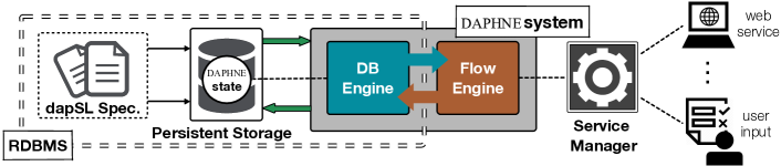
Figure 2: Conceptual architecture of daphne

3.1 Internal Architecture

The core architecture of daphne is depicted in Figure 2. The system takes as input a representation of a 𝕕𝕒𝕡𝕊𝕃 specification (or model) and uses a standard DBMS to support its execution.

The DBMS takes care of storing the data relevant to the input 𝕕𝕒𝕡𝕊𝕃 model and supports, through the DB Engine of the underlying DBMS, the application of a set of operations that jointly realize the given 𝕕𝕒𝕡𝕊𝕃 actions. The Flow Engine constitutes the application layer of the system; it facilitates the execution of a 𝕕𝕒𝕡𝕊𝕃 model by coordinating the activities that involve the user, the DBMS, and the services. Specifically, the Flow Engine issues queries to the DBMS, calls stored procedures, and handles the communication with external services through a further module called Service Manager.

Next we give a detailed representation of daphne’s architecture by describing the stages of each execution step. For the moment we do not consider how the input 𝕕𝕒𝕡𝕊𝕃 specification is concretely encoded inside the DBMS. At each point in time, the DBMS stores the current state of the 𝕕𝕒𝕡𝕊𝕃 model. We assume that, before the execution starts, the DBMS contains an initial database instance for the data layer of 𝕕𝕒𝕡𝕊𝕃 model. To start the execution, the Flow Engine queries the DBMS about the actions that are enabled in the current state; if one is found, the engine retrieves all possible parameter assignments that can be selected to ground the action, and returns them to the user (or the software module responsible for the process enactment). The user is then asked to choose one of such parameter assignments. At this point, the actual application of the ground action is triggered. The Flow Engine invokes a set of stored procedures from the DBMS that take care of evaluating and applying action effects. If needed by the action specification, the Flow Engine interacts with external services, through the Service Manager, to acquire new data via service calls. The tuples to be deleted and inserted in the various relations of the 𝕕𝕒𝕡𝕊𝕃 model are then computed, and the consequent changes are pushed to the DBMS within a transaction, so that the underlying database instance is updated only if all constraints are satisfied. After the update is committed or rolled back, the action execution cycle can be repeated by selecting either a new parameter assignment or another action available in the newly generated state.

(a)

(b)

(c)

Figure 3: The three main usage modalities for daphne, and sketch of the corresponding data structures stored within the DBMS

3.2 Encoding a 𝕕𝕒𝕡𝕊𝕃 in daphne

We now detail how daphne encodes a 𝕕𝕒𝕡𝕊𝕃 model 𝕕𝕒𝕡𝕊𝕃 model $\mathcal{S}=\langle\mathcal{L},\mathcal{P}\rangle$ with data layer $\mathcal{L}=\langle\mathcal{R},\mathcal{E}\rangle$ and control layer $\mathcal{P}=\langle\mathcal{F},\mathcal{A},\rho\rangle$ into a DBMS. Intuitively daphne represents $\mathcal{L}$ as a set of tables, and $\mathcal{P}$ as a set of stored procedures working over those and auxiliary tables. Such data structures and stored procedures are defined in terms of the native language of the chosen DBMS. These can be either created manually, or automatically instrumented by daphne itself once the user communicates to daphne the content of $\mathcal{S}$ using dedicated JAVA APIs. Specifically, we employ the jOOQ framework as the basis for the concrete input syntax of 𝕕𝕒𝕡𝕊𝕃 models within daphne. The interested reader may refer to Appendix 0.A to have a glimpse about how jOOQ and the DAPHNE APIs work.

Before entering into the encoding details, it is important to stress that daphne provides three main usage modalities. The first modality is enactment. Here daphne supports users in the process execution, storing the current DB, and suitably updating it in response to the execution of actions. The second modality is enactment with historical recall. This is enactment where daphne does not simply store the current state and evolves it, but also recalls historical information about the previous state configurations, i.e., the previous DBs, together with information about the applied actions (name, parameters, service call invocations and results, and timestamps). This provides full traceability about how the process execution evolved the initial state into the current one. The last modality is state space construction for formal analysis, where daphne generates all possible “relevant" possible executions of the system, abstracting away from timestamps and consequently folding the so-obtained traces into a relational transition system [25, 4]. Differently from the previous modalities, in this case daphne does not simply account for a system run, but for the branching behaviour of $\mathcal{S}$.

Figure 4: Relational schemas of $\mathit{CurrReq}$ and $\mathit{TrvlMaxAmnt}$, and their historical representation in daphne via two pairs of corresponding tables: $\mathit{CurrReq}_{\mathtt{raw}}$ and $\mathit{CurrReq}_{\mathtt{log}}$, $\mathit{TrvlMaxAmnt}_{\mathtt{raw}}$ and $\mathit{TrvlMaxAmnt}_{\mathtt{log}}$.

Data layer. daphne does not internally store the data layer as it is specified in $\mathcal{L}$, but adopts a more sophisticated schema. This is done to have a unique homogeneous approach that supports the three usage modalities mentioned before. In fact, instructing the DBMS to directly store the schema expressed in $\mathcal{L}$ would suffice only in the enactment case, but not to store historical data about previous states, nor the state space with its branching nature. To accommodate all three usages at once, daphne proceeds as follows. Each relation schema $\mathit{R}$ of $\mathcal{L}$ becomes relativized to a state identifier, and decomposed into two interconnected relation schemas: (i) $\mathit{R}_{\mathtt{raw}}$(raw data storage), an inflationary table that incrementally stores all the tuples that have been ever inserted in $\mathit{R}$; (ii) $\mathit{R}_{\mathtt{log}}$(state log), which is responsible at once for maintaining the referential integrity of the data in a state, as well as for fully reconstructing the exact content of $\mathit{R}$ in a state. In details, $\mathit{R}_{\mathtt{raw}}$ contains all the attributes $A$ of $\mathit{R}$ that are not part of primary keys nor sources of a foreign key, plus an additional surrogate identifier RID, so that $\textsc{pk}(\mathit{\mathit{R}_{\mathtt{raw}}})=\langle\textsf{RID}\rangle$. Each possible combination of values over $A$ is stored only once in $\mathit{R}_{\mathtt{raw}}$ (i.e., $\mathit{\mathit{R}_{\mathtt{raw}}}[A]$ is a key), thus maximizing compactness. At the same time, $\mathit{R}_{\mathtt{log}}$ contains the following attributes: (i) an attribute state representing the state identifier; (ii) the primary key of (the original relation) $R$; (iii) a reference to $\mathit{R}_{\mathtt{raw}}$, i.e., an attribute RID with $\mathit{\mathit{R}_{\mathtt{log}}}[\textsf{RID}]\rightarrow\mathit{\mathit{R}_{\mathtt{raw}}}[\textsf{RID}]$; (iv) all attributes of $\mathit{R}$ that are sources of a foreign key in $\mathcal{L}$. To guarantee referential integrity, $\mathit{R}_{\mathtt{log}}$ must ensure that (primary) keys and foreign keys are now relativized to a state. This is essential, as the same tuple of $R$ may evolve across states, consequently requiring to historically store its different versions, and suitably keep track of which version refers to which state. Also foreign keys have to be understood within the same state: if a reference tuple changes from one state to the other, all the other tuples referencing it need to update their references accordingly. To realize this, we set $\textsc{pk}(\mathit{R_{\mathtt{log}}})=\langle\textsc{pk}(\mathit{R}),\textsf{state}\rangle$. Similarly, for each foreign key $\mathit{\mathit{S}}[B]\rightarrow\mathit{\mathit{R}}[A]$ originally associated to relations $\mathit{R}$ and $\mathit{S}$ in $\mathcal{L}$, we insert in the DBMS the foreign key $\mathit{\mathit{S}_{\mathtt{log}}}[B,\textsf{state}]\rightarrow\mathit{\mathit{R}_{\mathtt{log}}}[A,\textsf{state}]$ over their corresponding state log relations.

With this strategy, the “referential" part of $\mathit{R}$ is suitably relativized w.r.t. a state, while at the same time all the other attributes are compactly stored in $\mathit{R}_{\mathtt{raw}}$, and referenced possibly multiple times from $\mathit{R}_{\mathtt{log}}$. In addition, notice that, given a state identified by $\mathtt{s}$, the full extension of relation $\mathit{R}$ in $\mathtt{s}$ can be fully reconstructed by (i) selecting the tuples of $\mathit{R}_{\mathtt{log}}$ where $\textsf{state}=\mathtt{s}$; (ii) joining the obtained selection with $\mathit{R}_{\mathtt{raw}}$ on RID; (iii) finally projecting the result on the original attributes of $\mathit{R}$. In general, this technique shows how an arbitrary SQL query over $\mathcal{L}$ can be directly reformulated as a state-relativized query over the corresponding daphne schema.

Example 4

Consider relation schemas $\mathit{CurrReq}$ and $\mathit{TrvlMaxAmnt}$ in Figure 10. Figure 4 shows the representation of these relations in daphne, suitably pairing $\mathit{CurrReq}_{\mathtt{raw}}$ with $\mathit{CurrReq}_{\mathtt{log}}$, and $\mathit{TrvlMaxAmnt}_{\mathtt{raw}}$ with $\mathit{TrvlMaxAmnt}_{\mathtt{log}}$. Each state log table directly references a corresponding raw data storage table (e.g., $\mathit{\mathit{CurrReq}_{\mathtt{log}}}[\mathsf{RID}]\rightarrow\mathit{\mathit{CurrReq}_{\mathtt{raw}}}[\mathsf{RID}]$), and $\mathit{TrvlMaxAmnt}$’s state log table, due to the FK in the original DAP, will reference a suitable key of $\mathit{CurrReq}_{\mathtt{log}}$ (i.e., $\mathit{TrvlMaxAmnt_{\mathtt{log}}}[\mathsf{state},\mathsf{FID}]\rightarrow\mathit{CurrReq_{\mathtt{log}}}[\mathsf{state},\mathsf{ID}]$). Figures 5, 6 and 7 show the evolution of the DBMS in response to the application of three ground actions, with full history recall. $\triangleleft$

Figure 5: Action application with two partial database snapshots mentioning $\mathit{Pending}$ and $\mathit{CurrReq}$. Here, $\mathtt{StartWorkflow}$ is applied in state $\mathtt{1}$ with $\{{\color[rgb]{0.2,0.2,1}\mathsf{id}}=\mathtt{2},{\color[rgb]{0.2,0.2,1}\mathsf{empl}}=\mathtt{Kriss},{\color[rgb]{0.2,0.2,1}\mathsf{dest}}=\mathtt{Paris}\}$ as binding and, in turn, generates a new state $\mathtt{2}$.

We now discuss updates over $\mathit{R}$. As already pointed out, $\mathit{R}_{\mathtt{raw}}$ stores any tuple that occurs in some state, that is, tuples are never deleted from $\mathit{R}_{\mathtt{raw}}$. Deletions are simply obtained by not referencing the deleted tuple in the new state. For instance, in Figure 5, it can be seen that the first tuple of $\mathit{Pending_{\mathtt{raw}}}$ (properly extended with its ID, through RID) has been deleted from $\mathit{Pending}$ in state $\mathtt{2}$: while being present in state $\mathtt{1}$ (cf. first tuple of $\mathit{Pending}_{\mathtt{log}}$), the tuple is not anymore in state $\mathtt{2}$ (cf. third tuple of $\mathit{Pending}_{\mathtt{log}}$).

Figure 6: Action application with two partial database snapshots mentioning $\mathit{CurrReq}$ and $\mathit{TrvlMaxAmnt}$. Here, $\mathtt{RvwRequest}$ is applied in state $\mathtt{2}$ with $\{{\color[rgb]{0.2,0.2,1}\mathsf{id}}=\mathtt{2},{\color[rgb]{0.2,0.2,1}\mathsf{empl}}=\mathtt{Kriss},{\color[rgb]{0.2,0.2,1}\mathsf{dest}}=\mathtt{Paris}\}$ as binding and $\mathtt{900}$ resulting from the invocation to service $\mathtt{@maxAmnt}$ that, in turn, generates a new state $\mathtt{3}$.

As for additions, we proceed as follows. Before inserting a new tuple, we check whether it is already present in $\mathit{R}_{\mathtt{raw}}$. If so, we update only $\mathit{R}_{\mathtt{log}}$ by copying the $\mathit{R}_{\mathtt{log}}$ tuple referencing the corresponding RID in $\mathit{R}_{\mathtt{raw}}$. In the copied tuple, the value of attribute state is going to be the one of the newly generated state, while the values of ID and all foreign key attributes remain unchanged. If the tuple is not present in $\mathit{R}_{\mathtt{raw}}$, it is also added to $\mathit{R}_{\mathtt{raw}}$ together with a fresh RID. Notice that in that case its ID and FK attributes are provided as input, and thus they are simply added, together with the value of state, to $\mathit{R}_{\mathtt{log}}$. In the actual implementation, $\mathit{R}_{\mathtt{raw}}$ features also a hash attribute, with the value of a hash function computed based on original $\mathit{R}$ attributes (extracted from both $\mathit{R}_{\mathtt{raw}}$ and $\mathit{R}_{\mathtt{log}}$). This speeds up the search for identical tuples in $\mathit{R}_{\mathtt{raw}}$.

Figure 7: Action application with three partial DB snapshots mentioning $\mathit{CurrReq}$, $\mathit{TrvlMaxAmnt}$ and $\mathit{TrvlCost}$. Here, $\mathtt{FillReimb}$ is applied in state $\mathtt{3}$ with $\{{\color[rgb]{0.2,0.2,1}\mathsf{id}}=\mathtt{2},{\color[rgb]{0.2,0.2,1}\mathsf{empl}}=\mathtt{Kriss},{\color[rgb]{0.2,0.2,1}\mathsf{dest}}=\mathtt{Paris}\}$ as binding and $\mathtt{700}$ resulting from the invocation of service $\mathtt{@cost}$ that, in turn, generates a new state $\mathtt{4}$.

Finally, we consider the case of relation schemas whose content is not changed when updating a state to a new state. Assume that relation schema $\mathit{S}$ stays unaltered. After updating $\mathit{R}$, it is enough to update $\mathit{S}_{\mathtt{log}}$ by copying previous state entries and updating the value of their state id to the actual one. If a FK, whose left-hand side is $\mathit{\mathit{S}}[B]$, belongs to $\mathcal{L}$ , the pair $\langle B,\textsf{state}\rangle$ will reference the most recent versions of the previously referenced tuples. Consider, e.g., Figure 7. While in his current request $\mathtt{Kriss}$ is changing the request status when moving from state $\mathtt{3}$ to state $\mathtt{4}$, the maximum traveling budget assigned to this request (a tuple in $\mathit{TrvlMaxAmnt}$) should reference the latest version of the corresponding tuple in $\mathit{CurrReq}$. Indeed, in state $\mathtt{4}$, a new tuple in $\mathit{TrvlMaxAmnt}_{\mathtt{log}}$ is referencing a new tuple in $\mathit{CurrReq}_{\mathtt{log}}$ that, in turn, corresponds to the one with the updated request status.

Control layer. Each action of $\mathcal{P}$, together with its dedicated CA rule, is encoded by daphne into three stored procedures. The encoding is quite direct, thanks to the fact that both action conditions and action effect specifications are specified using SQL.

The first stored procedure, _ca_eval(s), evaluates the CA rule of in state s over the respective DB (obtained by inspecting the state log relations whose state column matches with s), and stores the all returned parameter assignments for in a dedicated table _params. All parameter assignments in _params are initially unmarked, meaning that they are available for the user to choose. The second stored procedure, _eff_eval(s,b), executes queries corresponding to all the effects of over the DB of state s, possibly using action parameters from _params extracted via a binding identifier b. Query results provide values to instantiate service calls, as well as those facts that must be deleted from or added to the current DB. The third stored procedure, _eff_exec(s,b), transactionally performs the actual delete and insert operations for a given state s and a binding identifier b, using the results of service calls.

We describe now in detail the daphne action execution cycle in a given state s. (1) The cycle starts with the user choosing one of the available actions presented by the Flow Engine. The available actions are acquired by calling _ca_eval(s), for each action in $\mathcal{P}$. (2) If any unmarked parameter is present in _params, the user is asked to choose one of those (by selecting a binding identifier b); once chosen, the parameter is marked, and the Flow Engine proceeds to the evaluation of by calling _eff_eval(s,b). If there are no such parameters, the user is asked to choose another available action, and the present step is repeated. (3) If _eff_eval(s,b) involves service calls, these are passed to the the Service Manager component, which fetches the corresponding results. (4) _eff_exec(s,b)is executed. If all constraints in $\mathcal{L}$ are satisfied, the transaction is committed and a new iteration starts from step 1; otherwise, the transaction is aborted and the execution history is kept unaltered, and the execution continues from step 2.

3.3 Realization of the Three Usage Modalities

Let us now discuss how the three usage modalities are realized in daphne. The simple enactment modality is realized by only recalling the current information about log relations. Enactment with history recall is instead handled as follows. First, the generation of a new state always comes with an additional update over an accessory 1-tuple relation schema indicating the timestamp of the actual update operation. The fact that timestamps always increase along the execution guarantees that each new state is genuinely different from previously encountered ones. Finally, an additional binary state transition table is employed, so as to keep track of the resulting total order over state identifiers. By considering our running example, in state $\mathtt{4}$ shown in Figure 7, the content of the transition table would consist of the three pairs $\langle\mathtt{1},\mathtt{2}\rangle$, $\langle\mathtt{2},\mathtt{3}\rangle$, and $\langle\mathtt{3},\mathtt{4}\rangle$.

As for state space construction, some preliminary observations are needed. Due to the presence of external services that may inject fresh input data, there are in general infinitely many different executions of the process, possibly visiting infinitely many different DBs (differing in at least one tuple). In other words, the resulting relational transition systems has infinitely many different states. However, thanks to the correspondence between 𝕕𝕒𝕡𝕊𝕃 and DCDSs, we can realize in daphne the abstraction techniques that have been introduced in [1, 4] to attack the verification of such infinite-state transition systems. The main idea behind such abstraction techniques is the following. When carrying out verification, it is not important to observe all possible DBs that can be produced by executing the available actions with all possible service call results, but it suffices to only consider meaningful combination of values, representing all possible ways to relate tuples with other tuples in the DB, in terms of (in)equality of their different components. This is done by carefully selecting the representative values. In [1, 4], it has been shown that this technique produces a faithful representation of the original relational transition system, and that this representation is also finite if the original system is state bounded, that is, has a pre-defined (possibly unknown) bound on the number of tuples that can be stored therein. Constructing such a faithful representation is therefore the key towards analysis of formal properties such as reachability, liveness, and deadlock freedom, as well as explicit temporal model checking (in the style of [4]).

State space construction is smoothly handled in daphne as follows. When executed in this mode, daphne replaces the service call manager with a mock-up manager that, whenever a service call is invoked, returns all and only meaningful results, in the technical sense described above. E.g., if the current DB only contains string $\mathsf{a}$, invoking a service call that returns a string may only give two interesting results: $\mathsf{a}$ itself, or a string different than $\mathsf{a}$. To cover the latter case, the mock-up manager picks a representative value, say $\mathsf{b}$ in this example, implementing the representative selection strategy defined in [1, 4]. With this mock-up manager in place, daphne constructs the state space by executing the following iteration. A state s is picked (at the beginning, only the initial state exists and can be picked). For each enabled ground action in s, and for all relevant possible results returned by the mock-up manager, the DB instance corresponding to the update is generated. If such a DB instance has been already encountered (i.e., is associated to an already existing state), then the corresponding state id $\textsf{s}^{\prime}$ is fetched. If this is not the case, a new id $\textsf{s}^{\prime}$ is created, inserting its content into the DBMS. Recall that $\textsf{s}^{\prime}$ is not a timestamp, but just a symbolic, unique state id. The state transition table is then updated, by inserting the tuple $\langle\textsf{s},\textsf{s}^{\prime}\rangle$, which indeed witnesses that $\textsf{s}^{\prime}$ is one of the successors of s. The cycle is then repeated until all states and all enabled ground actions therein are processed. Notice that, differently from the enactment with history recall modality, in this case the state transition table is graph-structured, and in fact reconstructs the abstract representation of the relational transition system capturing the execution semantics of $\mathcal{S}$.

Figure 8 graphically depicts the state space constructed by daphne on the travel reimbursement process whose initial DB only contains a single pending request. More detailed examples on the state space construction for the travel reimbursement process can be found in Appendix 0.B.

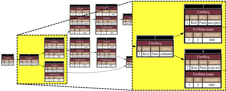
Figure 8: Example of state space constructed by daphne

4 Discussion and Related Work

Our approach directly relates to the family of data- and artifact-centric approaches [3] that inspired the creation of various modeling languages [9, 13] and execution frameworks such as: (i) the declarative rule-based Guard-Stage-Milestone (GSM) language [5] and its BizArtifact (https://sourceforge.net/projects/bizartifact/) execution platform; (ii) the OMG CMMN standard for case handling (https://www.omg.org/spec/CMMN/); (iii) the object-aware business process management approach implemented by PHILharmonic Flows [11]; (iv) the extension of GSM called EZ-Flow [26], with SeGA as [24] an execution platform; (v) the declarative data-centric process language Reseda based on term rewriting systems [21]. As opposed to the more traditional activity-centric paradigms, these approaches emphasize the evolution of data objects through different states, but often miss a clear representation of the control-flow dimension. For example, GSM provides means for specifying business artifact lifecycles in a declarative rule-based manner, and heavily relies on queries (ECA rules) over the data to implicitly define the allowed execution flows. Similarly, our 𝕕𝕒𝕡𝕊𝕃 language treats data as a “first-class citizen” and allows one to represent data-aware business processes from the perspective of database engineers. Other examples in (ii)–(iv) are rooted in similar abstractions to those of GSM, extending it towards more sophisticated interaction mechanisms between artifacts and their lifecycle components.

Our 𝕕𝕒𝕡𝕊𝕃 language departs from these abstractions and provides a very pristine, programming-oriented solution that only retains the notions of data, actions, and CA rules. In this respect, the closes approach to ours among the aforementioned ones is Reseda. Similarly to 𝕕𝕒𝕡𝕊𝕃, Reseda in general allows one to specify reactive rules and behavioral constraints defining the progression of a process in terms of data rewrites and data inputs from outside the process context. Reseda manipulates only semi-structured data (such as XML or JSON) that have to be specified directly in the tool. 𝕕𝕒𝕡𝕊𝕃 focuses instead on purely relational data, and lends itself to be used on top of already specified relational DBs.

Differently from all such approaches, state-of-the-art business process management systems, along with an explicit representation of the process control flow, often provide sophisticated, ad-hoc conceptual abstractions to manipulate business data. Notable examples of such systems are the Bizagi BPM suite (bizagi.com), Bonita BPM (bonitasoft.com), Camunda (camunda.com), Activiti (activiti.org), and YAWL (yawlfoundation.org). While they all provide an explicit representation of the process control flow using similar, well-accepted abstractions, they typically consider the task logic and its interaction with persistent data as a sort of “procedural attachment”, i.e., a piece of code whose functioning is not conceptually revealed [3]. This is also apparent in standard languages such as BPMN, which consider the task and the decision logics as black boxes. The shortcomings of this assumption have been extensively discussed in the literature [19, 7, 18, 3]. 𝕕𝕒𝕡𝕊𝕃, due to its pristine, data-centric flavor, can be used to complement such approaches with a declarative, explicitly exposed specification of the task and decision logic, using the well-accepted SQL language as main modeling metaphor.

5 Conclusions

We have introduced a declarative, purely relational framework for data- aware processes, in which SQL is used as the core data inspection and update language. We have reported on the implementation of this framework in DAPHNE, a system prototype grounded in standard relational technology and Java that at once accounts for modeling, enactment, and state space construction for verification. As for modeling, we intend to interface DAPHNE with different concrete end user- oriented languages for the integrated modeling of processes and data, incorporating at once artifact- and activity-centric approaches. Since our approach is having a minimalistic, SQL-centric flavor, it would be also interesting to empirically validate it and, in particular, to study its usability among database experts who need to model processes. Daphne could in fact allow them to enter into process modeling by using a metaphor that is closer to their expertise. As for formal analysis, we plan to augment the state space construction with native verification capabilities to handle basic properties such as reachability and liveness, and even more sophisticated temporal logic model checking. At the moment, the development of verification tools for data- aware processes is at its infancy, with a few existing tools [6, 12]. Finally, given that DAPHNE can generate a log including all performed actions and data changes, we aim at investigating its possible applications to process mining, where emerging trends are moving towards multi-perspective analyses that consider not just the sequence of events but also the corresponding data.

Appendix 0.A Interacting with daphne

daphne comes with dedicated APIs to acquire a DAPS, injects it in the underlying DBMS, and interact with the execution engine, on the one hand inspect the state of the process and the current data, and on the other to enact its progression. In order to avoid redundant technicalities and still give a flavor of the way daphne works, we show how to specify and enact DAPSs on top of it for the case when the history recall modality is chosen.

As a concrete specification language for DAPS, we are developing an extension of the standard SQL, mixed with few syntactic additions allowing to compactly define DAPS rules and actions. Concretely, such a language is directly embedded into Java using the jOOQ framework, which allows to create and manipulate relational tables, constraints, and SQL queries as Java objects. Building on top of the JOOQ APIs, we have realized an additional API layer that, given a jOOQ object describing a DAPS component (such as a relation, rule, or action), automatically transforms it into a corresponding SQL or PL/pgSQL code snippet following the strategy defined in Section 3.2. E.g., one could specify the $\mathit{CurrReq}$ schema and its primary key using the following code:

⬇

1DSLContext create = DSL.using(SQLDialect.POSTGRES_9_4);

2Field<Integer> id = DSL.field(DSL.name("CurrReq", "id"),

3 SQLDataType.INTEGER.nullable(false).identity(true));

4Field<String> empl = DSL.field(DSL.name("CurrReq", "empl"),

5 SQLDataType.VARCHAR.length(40).nullable(false));

6Field<String> dest = DSL.field(DSL.name("CurrReq", "dest"),

7 SQLDataType.VARCHAR.length(40).nullable(false));

8Field<String> status = DSL.field(DSL.name("CurrReq", "status"),

9 SQLDataType.VARCHAR.length(40).nullable(false));

10Schema currReq = new Schema("CurrReq", id, empl, dest, status);

11PrimaryKey pkCurrReq = new PrimaryKey("pk_CurrReq", currReq,

12 Arrays.asList(id));

13currReq.addConstraint(pkCurrReq);

To generate the SQL code for that relation, which should account for creating the state log and raw data storage relations for $\mathit{CurrReq}$ (and related constraints), one can then either rely on conventional JDBC methods, or directly invoke the daphne API:

⬇

1String createCurrReq_script = currReq.getSQLTranslation(create);

The following snippet shows how to create a CA rule for action $\mathtt{RvwRequest}$:

⬇

1Select query = create.select(id,empl, dest)

2 .from(currReq.generateTable(), trvlCost.generateTable())

3 .where(status.eq("submitted"));

4Action rvwRequest = new Action("RvwRequest");

5CARule rvwRequestCARule = new CARule(query, rvwRequest);

To generate a script that will instrument the necessary tables and stored procedures in the underlying DAPS, as stipulated in Section 3.2, the user just needs to call another dedicated daphne API:

⬇

1String script = rvwRequestCARule.getSQLTranslation(create);

Let us now provide a flavour of the runtime API of daphne, employed during the enactment of a system run. First, we need to obtain an instance of process engine, providing its corresponding database connection details:

⬇

1Connection con = DBTools.getConnection(...);

2StatefulEngine dcds = StatefulEngine.getEngingeInstance(con);

The engine provides a plethora of state inspection and update functionalities. We show how to create an action provider object that provides metadata (such as action names and their params) about all actions that are enabled in the current state.

⬇

1State currState = dcds.getCurrentState();

2ActionProvider provider = dcds.getActionProvider(currState);

3List<Attributes> md = provider.getAvailableActionsMetaData();

Using one of the so-obtained metadata, we create an action and a binding provider, in turn used to obtain all the current legal parameter instantiations for such an action.

⬇

1Attributes att = md.get(0);

2ImmutablePair<Action, BindingProvider> actionElements

3 = provider.getAction(att);

Among the available bindings, we pick one, getting back a ground, “ready-to-fire” action that can then be transactionally applied by daphne.

⬇

1List<Binding> bindings

2 = actionElements.getRight().getAvailableBindings();

3GroundAction groundAction

4 = actionElements.getLeft().bind(bindings.get(0));

With this ground action at hand, we can check whether it involves service calls in its specification. Service calls are responsible for the communication with the outer world and might introduce some fresh data into the system. In the database, every service call invocation is represented as a textual signature. E.g., the service call $\mathtt{@maxAmnt}$ on employee $\mathtt{Kriss}$ with trip destination $\mathtt{Rome}$ is internally represented as a string $\mathtt{maxAmnt(Kriss,Rome)}$ in the database. daphne knows about this internal representation and offers a special storage for all the service call invocations, i.e., a service call map list. This list keeps a map from services to all their invocations in the state. Each invocation also comes with the value type that the original service call returns.

⬇

1ServiceCallMapList aSCMList = groundAction.getServiceCallMapList();

If the evaluation of ground action effects yielded at least one service invocation , one has to instantiate it before updating the database. To do so we create a service manager instance that, given a service call map list, manages corresponding service objects by applying them to processed arguments (extracted from the signatures) and then collecting the results of the invocations. As soon as the service call map list is fully instantiated, one can finally proceed with executing the ground action

⬇

1ServiceManager sm = new ServiceManager(connection);

2if (!aSCMList.equals(null)) {

3 aSCMList = sm.getResults(aSCMList,currState.getStateID());}

4groundAction.launch(aSCMList);

Appendix 0.B State-space construction

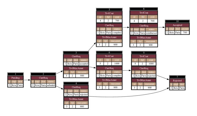
Figure 9: State space of the travel reimbursement process with one pending request

A complete example of the state space (cf. Figure 8) of the travel reimbursement with only one pending request $\mathit{Pending}(\mathtt{2},\mathtt{Kriss},\mathtt{Paris})$ is present in Figure 9. For ease of presentation, we assume that the maximum reimbursable amount $\mathtt{500}$ and, without loss of generality, we also restrict the range of cost to 400, 600. Like that one can easily model two scenarios: when a reimbursement request is accepted (i.e., the travel cost is less or equal than the maximum reimbursable amount) and when it is rejected (i.e., the travel cost is greater than the maximum reimbursable amount).

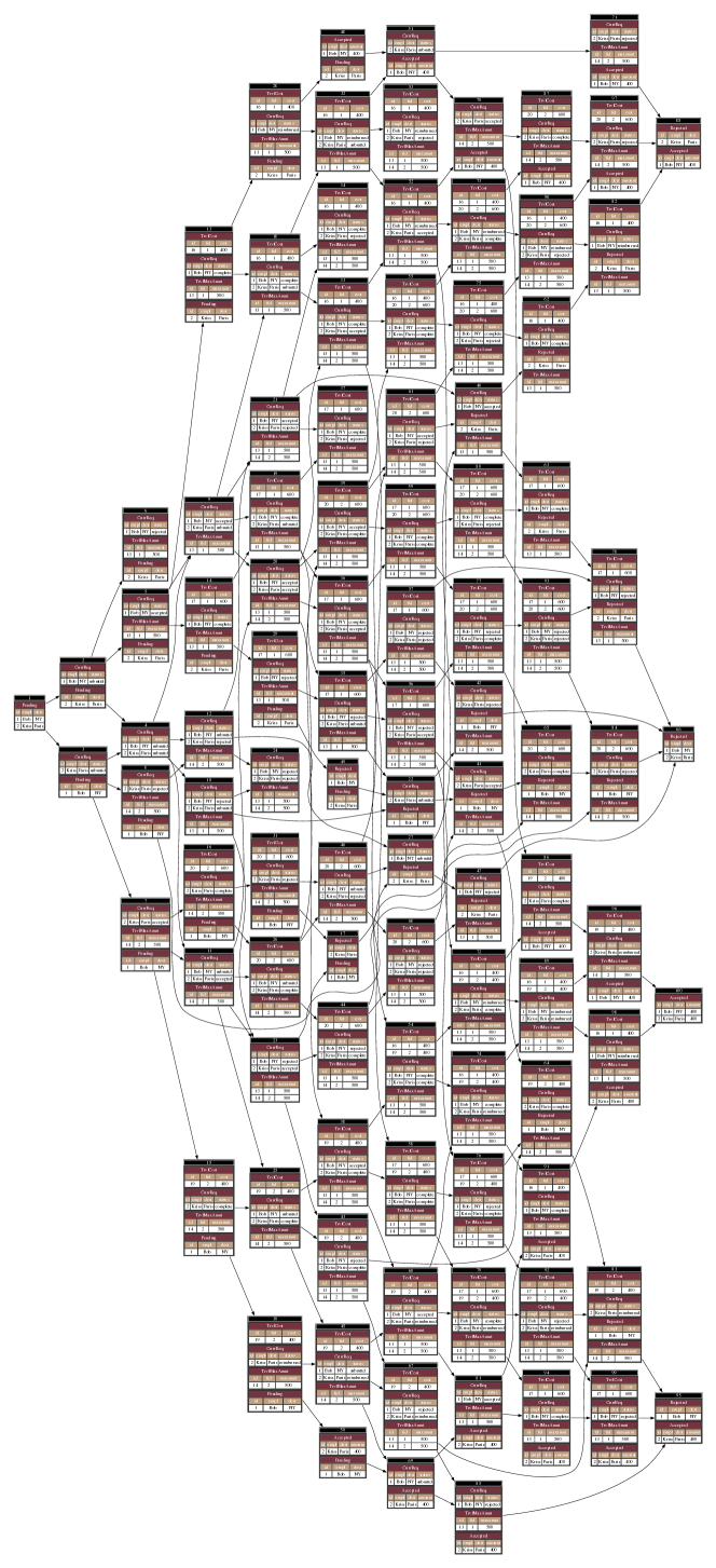
Figure 10: State space of the travel reimbursement process with two pending requests

The next example, analogously to Section 3.2 considers two pending requests $\mathit{Pending}(\mathtt{1},\mathtt{Bob},\mathtt{NY})$ and $\mathit{Pending}(\mathtt{2},\mathtt{Kriss},\mathtt{Paris})$. The corresponding state space can bee seen in Figure 10. Given that the travel reimbursement workflow (cf. Figure ) does not consider any interaction between different process instances, it is enough to see each of such instances evolving “in isolation”, that is, assuming the same execution scenario (with the same maximum amount an travel cost values) as above. Like that, the state space becomes nothing but a set of all possible combinations of states of two process instances.

References

- [1] Bagheri Hariri, B., Calvanese, D., De Giacomo, G., Deutsch, A., Montali, M.: Verification of relational data-centric dynamic systems with external services. In: Proc. of PODS (2013)
- [2] Bagheri Hariri, B., Calvanese, D., Deutsch, A., Montali, M.: State-boundedness for decidability of verification in data-aware dynamic systems. In: Proc. of KR. AAAI Press (2014)
- [3] Calvanese, D., De Giacomo, G., Montali, M.: Foundations of data aware process analysis: A database theory perspective. In: Proc. of PODS (2013)
- [4] Calvanese, D., De Giacomo, G., Montali, M., Patrizi, F.: First-order -calculus over generic transition systems and applications to the situation calculus. Inf. and Comp. 259(3), 328–347 (2018). https://doi.org/10.1016/j.ic.2017.08.007
- [5] Damaggio, E., Hull, R., Vaculín, R.: On the equivalence of incremental and fixpoint semantics for business artifacts with Guard-Stage-Milestone lifecycles. In: Proc. of BPM (2011)
- [6] De Masellis, R., Di Francescomarino, C., Ghidini, C., Montali, M., Tessaris, S.: Add data into business process verification: Bridging the gap between theory and practice. In: Proc. of AAAI. AAAI Press (2017)
- [7] Dumas, M.: On the convergence of data and process engineering. In: Proc. of ADBIS. LNCS, vol. 6909. Springer (2011)
- [8] Furtado, A.L., Casanova, M.A.: Updating relational views. In: Query Processing in Database Systems, pp. 127–142. Springer (1985)
- [9] Hull, R.: Artifact-centric business process models: Brief survey of research results and challenges. In: Proc. of OTM. LNCS, vol. 5332. Springer (2008)
- [10] Köpke, J., Su, J.: Towards quality-aware translations of activity-centric processes to guard stage milestone. In: Proc. of BPM. LNCS, vol. 9850. Springer (2016)
- [11] Künzle, V., Weber, B., Reichert, M.: Object-aware business processes: Fundamental requirements and their support in existing approaches. Int. J. of Information System Modeling and Design 2(2) (2011)
- [12] Li, Y., Deutsch, A., Vianu, V.: VERIFAS: A practical verifier for artifact systems. PVLDB 11(3) (2017)
- [13] Meyer, A., Smirnov, S., Weske, M.: Data in business processes. Tech. Rep. 50, Hasso-Plattner-Institut for IT Systems Engineering, Universität Potsdam (2011)
- [14] Montali, M., Calvanese, D.: Soundness of data-aware, case-centric processes. Int. J. on Software Tools for Technology Transfer 18(5), 535–558 (2016)
- [15] Montali, M., Rivkin, A.: Model checking Petri nets with names using data-centric dynamic systems. Formal Aspects of Computing (2016)
- [16] Montali, M., Rivkin, A.: DB-Nets: on the marriage of colored Petri Nets and relational databases. Trans. on Petri Nets and Other Models of Concurrency 28(4) (2017)
- [17] Olivé, A.: Conceptual modeling of information systems. Springer (2007)
- [18] Reichert, M.: Process and data: Two sides of the same coin? In: Proc. of OTM. LNCS, vol. 7565. Springer (2012)
- [19] Richardson, C.: Warning: Don’t assume your business processes use master data. In: Proc. of BPM. LNCS, vol. 6336. Springer (2010)
- [20] Ritter, D., Rinderle-Ma, S., Montali, M., Rivkin, A., Sinha, A.: Formalizing application integration patterns. In: 22nd IEEE International Enterprise Distributed Object Computing Conference, EDOC 2018, Stockholm, Sweden, October 16-19, 2018. pp. 11–20 (2018). https://doi.org/10.1109/EDOC.2018.00012
- [21] Seco, J.C., Debois, S., Hildebrandt, T.T., Slaats, T.: RESEDA: declaring live event-driven computations as reactive semi-structured data. In: 22nd IEEE International Enterprise Distributed Object Computing Conference, EDOC 2018, Stockholm, Sweden, October 16-19, 2018. pp. 75–84 (2018). https://doi.org/10.1109/EDOC.2018.00020
- [22] Solomakhin, D., Montali, M., Tessaris, S., De Masellis, R.: Verification of artifact-centric systems: Decidability and modeling issues. In: Proc. of ICSOC. LNCS, vol. 8274. Springer (2013)
- [23] Sun, Y., Su, J., Wu, B., Yang, J.: Modeling data for business processes. In: Proc. of ICDE. pp. 1048–1059. IEEE Computer Society (2014)
- [24] Sun, Y., Su, J., Yang, J.: Universal artifacts: A new approach to business process management (BPM) systems. ACM TMIS 7(1) (2016)
- [25] Vardi, M.Y.: Model checking for database theoreticians. LNCS, vol. 3363, pp. 1–16. Springer (2005)
- [26] Xu, W., Su, J., Yan, Z., Yang, J., Zhang, L.: An artifact-centric approach to dynamic modification of workflow execution. In: Proc. of CoopIS. vol. 7044. Springer (2011)