Abstract

Unnormalised latent variable models are a broad and flexible class of statistical models. However, learning their parameters from data is intractable, and few estimation techniques are currently available for such models. To increase the number of techniques in our arsenal, we propose variational noise-contrastive estimation (VNCE), building on NCE which is a method that only applies to unnormalised models. The core idea is to use a variational lower bound to the NCE objective function, which can be optimised in the same fashion as the evidence lower bound (ELBO) in standard variational inference (VI). We prove that VNCE can be used for both parameter estimation of unnormalised models and posterior inference of latent variables. The developed theory shows that VNCE has the same level of generality as standard VI, meaning that advances made there can be directly imported to the unnormalised setting. We validate VNCE on toy models and apply it to a realistic problem of estimating an undirected graphical model from incomplete data.

1 Introduction

Building flexible statistical models and estimating them is a core task in unsupervised machine learning. For observed data $\{{\mathbf{x}}_{1},\ldots,{\mathbf{x}}_{n}\}$, parametric modelling involves specifying a family of probability density functions (pdfs) $\{p({\mathbf{x}};{\boldsymbol{\theta}})\}$ parametrised by ${\boldsymbol{\theta}}$ that has the capacity to capture the structure in the data. Two fundamental modelling techniques are (i) introducing latent variables which serve as explanatory factors or model missing data; and (ii) energy-based modelling which removes the constraint that each member of the family has to integrate to one, rendering the model unnormalised.

Both techniques are widely used. Latent variable models have generated excellent results in an array of tasks, such as semi-supervised modelling of image data (Kingma et al.,, 2014) and topic modelling of text corpora (Hoffman et al.,, 2013). In addition, many real-world data sets are incomplete, and it is advantageous to model the missing values probabilistically as latent variables (e.g. Jordan et al.,, 1999; Nazabal et al.,, 2018). Energy-based models — also known as unnormalised models — have led to several advances in e.g. neural language modelling (Mnih and Kavukcuoglu,, 2013), multi-label classification (Belanger and McCallum,, 2016) and unsupervised representation learning (Oord et al.,, 2018).

Despite their individual successes, there are few attempts in the literature to combine the two types of models, a notable exception being deep Boltzmann machines (Ruslan and Hinton,, 2009). This is primarily because learning the parameters of unnormalised latent variable models is very difficult. For both types of models, evaluating $p({\mathbf{x}};{\boldsymbol{\theta}})$ becomes intractable, and thus the combined case is doubly-intractable. For latent variable models, $p({\mathbf{x}};{\boldsymbol{\theta}})$ is only obtained after integrating out the latents ${\mathbf{z}}$

$$p({\mathbf{x}};{\boldsymbol{\theta}})=\int p({\mathbf{x}},{\mathbf{z}};{\boldsymbol{\theta}})\operatorname{d\!}{\mathbf{z}},$$ (1)

whilst for unnormalised models $\phi({\mathbf{x}};{\boldsymbol{\theta}})$, we have

$$p({\mathbf{x}};{\boldsymbol{\theta}})=\phi({\mathbf{x}};{\boldsymbol{\theta}})/Z({\boldsymbol{\theta}}),$$ (2)

where $Z({\boldsymbol{\theta}})=\int\phi({\mathbf{x}};{\boldsymbol{\theta}})\operatorname{d\!}{\mathbf{x}}$ is the normalising partition function. In both cases, the model $p({\mathbf{x}};{\boldsymbol{\theta}})$ is defined in terms of integrals that cannot be solved or easily approximated. And without access to $p({\mathbf{x}};{\boldsymbol{\theta}})$, we cannot learn ${\boldsymbol{\theta}}$ by standard maximum likelihood estimation.

One potential solution is to make use of the following expression of the gradient of the log-likelihood (for a data point ${\mathbf{x}}_{i}$)

$$\mathbb{E}_{{\mathbf{z}}\sim p({\mathbf{z}}\>|\>{\mathbf{x}}_{i};{\boldsymbol{\theta}})}\left[\nabla_{{\boldsymbol{\theta}}}\log\phi({\mathbf{x}}_{i},{\mathbf{z}};{\boldsymbol{\theta}})\right]-$$

$$\mathbb{E}_{{\mathbf{x}},{\mathbf{z}}\sim p({\mathbf{x}},{\mathbf{z}};{\boldsymbol{\theta}})}\left[\nabla_{{\boldsymbol{\theta}}}\log\phi({\mathbf{x}},{\mathbf{z}};{\boldsymbol{\theta}})\right]$$ (3)

and to perform stochastic ascent on the log-likelihood. This requires samples from $p({\mathbf{x}},{\mathbf{z}};{\boldsymbol{\theta}})$ and the posterior $p({\mathbf{z}}\>|\>{\mathbf{x}}_{i};{\boldsymbol{\theta}})$ which, for some models, can be obtained by Markov chain Monte Carlo.

However, this approach is not always practical, or even feasible, and so more specialised methods are being used for efficient parameter estimation. To handle latent variables, variational inference (Jordan et al.,, 1999) is a commonly used, powerful technique involving the maximisation of a tractable lower bound to the log-likelihood. For unnormalised models, specialised methods include score matching (Hyvärinen,, 2005), ratio matching (Hyvärinen,, 2007), contrastive divergence (CD, Hinton,, 2002), persistent contrastive divergence (Younes,, 1998; Tieleman and Hinton,, 2009) and noise-contrastive estimation (NCE, Gutmann and Hyvärinen,, 2012).

There are thus multiple estimating methods for either latent variable models or unnormalised models, but not for both and there has been little work on combining methods from the two camps. To our knowledge, the only combination available is (persistent) CD with variational inference (Ruslan and Hinton,, 2009). Whilst this combination has worked well in the context of Boltzmann machines, it is unclear how well these results generalise to other models. Given the limited number of existing methods, it is important to have more estimation techniques at our disposal.

We here develop a novel variational theory for NCE that enables parameter estimation of unnormalised, latent variable models. This method, VNCE, maximises a variational lower bound to the NCE objective. Just as with standard variational inference on the log-likelihood, VNCE both estimates the model parameters and yields a posterior distribution over latent variables. For parameter estimation, we prove that VNCE is, in a sense, equivalent to NCE and is theoretically well grounded. For approximate inference, we prove that VNCE minimises a f-divergence between the true and approximate posterior. We further prove that with increased use of computational resources, we can recover standard variational inference by pushing this f-divergence towards the usual Kullback-Leibler (KL) divergence.

Given the applicability of NCE in a wide range of domains such as natural language processing (NLP, e.g. Mikolov et al.,, 2013), recommendation systems (Huang et al.,, 2015), policy transfer learning (Zhang et al.,, 2016) etc. the ability to now incorporate latent variables into such models is an important advance. For instance, in NLP, latent variable models, such as topic models, are in widespread use (Kim et al.,, 2018). Moreover, missing data is a ubiquitous problem across many domains and, as we show experimentally in Section 5, modelling the missing values probabilistically with VNCE offers signficant gains compared to using NCE with standard fixed-imputation strategies.

2 Background

Noise-contrastive estimation (NCE, Gutmann and Hyvärinen,, 2012) is a method for estimating the parameters of unnormalised models $\phi({\mathbf{x}};{\boldsymbol{\theta}})$. The idea is to convert the unsupervised estimation problem into a supervised classification problem, by training a (non-linear) logistic classifier to distinguish between the observed data $\{{\mathbf{x}}_{1},\ldots,{\mathbf{x}}_{n}\}$, and $m$ auxiliary samples $\{\textbf{y}_{1},\ldots,\textbf{y}_{m}\}$ that are drawn from a user-specified ‘noise’ distribution $p_{\mathbf{y}}$.

Using the logistic loss, parameter estimation in NCE is done by maximising the sample version of $J_{\scaleto{\mathrm{NCE}}{4pt}}({\boldsymbol{\theta}})$,

$$J_{\scaleto{\mathrm{NCE}}{4pt}}({\boldsymbol{\theta}}) =\mathbb{E}_{{\mathbf{x}}}\log h({\mathbf{x}};{\boldsymbol{\theta}})+\nu\mathbb{E}_{{\mathbf{y}}}\log(1-h({\mathbf{y}};{\boldsymbol{\theta}})),$$ (4)

where $\nu=m/n$ and $h({\mathbf{u}};{\boldsymbol{\theta}})$ depends on the unnormalised model $\phi({\mathbf{u}};{\boldsymbol{\theta}})$ and the noise pdf $p_{\mathbf{y}}({\mathbf{u}})$,

$$h({\mathbf{u}};{\boldsymbol{\theta}}) =\frac{\phi({\mathbf{u}};{\boldsymbol{\theta}})}{\phi({\mathbf{u}};{\boldsymbol{\theta}})+\nu p_{\mathbf{y}}({\mathbf{u}})}.$$ (5)

Typically, the model is allowed to vary freely in scale which can always be achieved by multiplying it by $\exp(-c)$, where $c$ is a scaling parameter that we absorb into ${\boldsymbol{\theta}}$ and estimate along with the other parameters.

Gutmann and Hyvärinen, (2012) prove that the resulting estimator is consistent for unnormalised models. They further show that NCE approaches the performance of MLE as the ratio of noise to data samples $\nu$ increases (for stronger results, see Barthelmé and Chopin,, 2015; Riou-Durand and Chopin,, 2018). For generalisations of NCE to other than the logistic loss function, see (Pihlaja et al.,, 2010; Gutmann and Hirayama,, 2011; Barthelmé and Chopin,, 2015).

The noise distribution affects the efficiency of the NCE estimator. While simple distributions such as Gaussians or uniform distributions often work well (Mnih and Whye,, 2012), both intuition and empirical results suggest that the noise samples should be hard to distinguish from the data (Gutmann and Hyvärinen,, 2012). The choice of the noise distribution becomes particularly important for high-dimensional data or when the data is concentrated on a lower dimensional manifold. For recent work on choosing the noise semi-automatically, see Ceylan and Gutmann, (2018).

While NCE avoids the computation of the intractable partition function, it assumes that we have data available for all variables ${\mathbf{x}}$ in the model. This means that NCE is, in general, not applicable to latent variable models. It will only apply in the special case where we can marginalise out the latent variables, as e.g. in mixture models (Matsuda and Hyvarinen,, 2018). The fact that NCE cannot handle more general latent variable models is a major limitation that we address in this paper.

3 Variational noise-contrastive estimation

We here derive a variational lower bound on the NCE objective function, allowing us to estimate the parameters of unnormalised, latent variable models. We then provide theoretical guarantees for this novel type of variational inference.

3.1 NCE lower bound

We assume that we are given an unnormalised parametric model $\phi({\mathbf{x}},{\mathbf{z}};{\boldsymbol{\theta}})$ for the joint distribution of the observables ${\mathbf{x}}$ and the latent variables ${\mathbf{z}}$ (some of which may correspond to missing data). The unnnormalised pdf $\phi({\mathbf{x}};{\boldsymbol{\theta}})$ of the observables ${\mathbf{x}}$ is then defined via the (typically intractable) integral

$$\phi({\mathbf{x}};{\boldsymbol{\theta}})=\int\phi({\mathbf{x}},{\mathbf{z}};{\boldsymbol{\theta}})\operatorname{d\!}{\mathbf{z}}.$$ (6)

The NCE objective function $J_{\scaleto{\mathrm{NCE}}{4pt}}$ depends on $\phi({\mathbf{u}};{\boldsymbol{\theta}})$ through $\log h({\mathbf{u}};{\boldsymbol{\theta}})$, which occurs in the first term of $J_{\scaleto{\mathrm{NCE}}{4pt}}$, and $\log(1-h({\mathbf{u}};{\boldsymbol{\theta}}))$, which occurs in the second term of $J_{\scaleto{\mathrm{NCE}}{4pt}}$. For the first term, we can write

$$\log h({\mathbf{x}};{\boldsymbol{\theta}}) =\log\bigg{(}\frac{\int\phi({\mathbf{x}},{\mathbf{z}};{\boldsymbol{\theta}})\operatorname{d\!}{\mathbf{z}}}{\int\phi({\mathbf{x}},{\mathbf{z}};{\boldsymbol{\theta}})\operatorname{d\!}{\mathbf{z}}+\nu p_{\mathbf{y}}({\mathbf{x}})}\bigg{)}$$ (7)

$$=g(r({\mathbf{x}};{\boldsymbol{\theta}})),$$ (8)

where we introduced the notation

$$g(r) =-\log\bigg{(}1+\frac{\nu}{r}\bigg{)}, r({\mathbf{x}};{\boldsymbol{\theta}}) =\frac{\int\phi({\mathbf{x}},{\mathbf{z}};{\boldsymbol{\theta}})\operatorname{d\!}{\mathbf{z}}}{p_{\mathbf{y}}({\mathbf{x}})}.$$ (9)

Importantly, $g$ is a concave function of $r$ (see the supplementary material). Using importance sampling, we then rewrite $r$ as an expectation

$$r({\mathbf{x}};{\boldsymbol{\theta}})=\mathbb{E}_{{\mathbf{z}}\sim q({\mathbf{z}}\>|\>{{\mathbf{x}}})}\bigg{(}\frac{\phi({\mathbf{x}},{\mathbf{z}};{\boldsymbol{\theta}})}{q({\mathbf{z}}\>|\>{{\mathbf{x}}})p_{\mathbf{y}}({\mathbf{x}})}\bigg{)}$$ (10)

and apply Jensen’s inequality to obtain the bound

$$g(r({\mathbf{x}};{\boldsymbol{\theta}}))\geq\mathbb{E}_{{\mathbf{z}}\sim q({\mathbf{z}}\>|\>{{\mathbf{x}}})}g\bigg{(}\frac{\phi({\mathbf{x}},{\mathbf{z}};{\boldsymbol{\theta}})}{q({\mathbf{z}}\>|\>{{\mathbf{x}}})p_{\mathbf{y}}({\mathbf{x}})}\bigg{)}$$ (11)

$$\geq\mathbb{E}_{{\mathbf{z}}\sim q({\mathbf{z}}\>|\>{{\mathbf{x}}})}\log\bigg{(}\frac{\phi({\mathbf{x}},{\mathbf{z}};{\boldsymbol{\theta}})}{\phi({\mathbf{x}},{\mathbf{z}};{\boldsymbol{\theta}})+\nu q({\mathbf{z}}\>|\>{{\mathbf{x}}})p_{\mathbf{y}}({\mathbf{x}})}\bigg{)},$$ (12)

where the second line is obtained by substituting in the definition of $g$ and then rearranging. We note that this result does not follow from standard variational inference on the log-likelihood, however it leverages the same mathematical trick of importance sampling combined with Jensen’s inequality.

We now have a lower bound on the first, but not the second, term of the NCE objective $J_{\scaleto{\mathrm{NCE}}{4pt}}$. But this is actually sufficient: we can handle the intractable integral in the second term with importance sampling, re-using the same variational distribution $q$ that we use in the first term. The final objective, which we call the VNCE objective, is then given by:

$$J_{\scaleto{\mathrm{VNCE}}{4pt}}({\boldsymbol{\theta}},q) =\mathbb{E}_{{\mathbf{x}}}\mathbb{E}_{{\mathbf{z}}\sim q({\mathbf{z}}\>|\>{{\mathbf{x}}})}\log\bigg{(}\frac{\phi({\mathbf{x}},{\mathbf{z}};{\boldsymbol{\theta}})}{\phi({\mathbf{x}},{\mathbf{z}};{\boldsymbol{\theta}})+\nu q({\mathbf{z}}\>|\>{{\mathbf{x}}})p_{\mathbf{y}}({\mathbf{x}})}\bigg{)}$$

$$+\nu\mathbb{E}_{{\mathbf{y}}}\log\bigg{(}\frac{\nu p_{\mathbf{y}}({\mathbf{y}})}{\nu p_{\mathbf{y}}({\mathbf{y}})+\mathbb{E}_{{\mathbf{z}}\sim q({\mathbf{z}}\>|\>{\mathbf{y}})}\left[\frac{\phi({\mathbf{y}},{\mathbf{z}};{\boldsymbol{\theta}})}{q({\mathbf{z}}\>|\>{\mathbf{y}})}\right]}\bigg{)}.$$ (13)

In practice, we optimise the sample version of this, replacing expectations with Monte Carlo averages.

By construction, we have that $J_{\scaleto{\mathrm{NCE}}{4pt}}({\boldsymbol{\theta}})\geq J_{\scaleto{\mathrm{VNCE}}{4pt}}({\boldsymbol{\theta}},q)$ for all $q$ and this bound is tight when the variational distribution $q({\mathbf{z}}\>|\>{\mathbf{x}})$ equals the true posterior $p({\mathbf{z}}\>|\>{\mathbf{x}};{\boldsymbol{\theta}})$. Importantly, the true posterior is also the optimal proposal distribution in the second term (see supplementary material). Thus, we do not need to blindly guess a good proposal distribution; we obtain one automatically through maximising $J_{\scaleto{\mathrm{VNCE}}{4pt}}({\boldsymbol{\theta}},q)$ with respect to $q$. Finally, we note that, just as with NCE, the user must specify the noise distribution $p_{\mathbf{y}}$.

3.2 Theoretical guarantees

We here prove basic properties of VNCE and establish its connection to NCE and standard variational inference. Below we simply state the results; all proofs can be found in the supplementary material.

Standard variational inference (VI) minimises the KL-divergence between the approximate and true posterior. In contrast, we show that VNCE minimises a different f-divergence between the two posteriors.

Definition 1.

An f-divergence $D_{f}(p\;\|\;q)$ between two probability density functions $p$ and $q$, is defined as

$$D_{f}(p\;\|\;q)=\mathbb{E}_{u\sim q}\left[f\left(\frac{p(u)}{q(u)}\right)\right],$$ (14)

where $f$ is a convex function satisfying $f(1)=0$.

It follows from Jensen’s inequality that f-divergences are non-negative and obtain their minimum precisely when $p=q$. The KL divergence is an important example of an f-divergence, where $f(u)=u\log(u)$.

Lemma 1.

The difference between the NCE and VNCE objective functions is equal to the expectation of an f-divergence between the true and approximate posterior. Specifically,

$$J_{\scaleto{\mathrm{NCE}}{4pt}}({\boldsymbol{\theta}})-J_{\scaleto{\mathrm{VNCE}}{4pt}}({\boldsymbol{\theta}},q)=\mathbb{E}_{{\mathbf{x}}}\left[D_{f_{{\mathbf{x}}}}(p_{{\boldsymbol{\theta}}}({\mathbf{z}}\>|\>{\mathbf{x}})\;\|\;q({\mathbf{z}}\>|\>{\mathbf{x}}))\right],$$ (15)

where

$$f_{{\mathbf{x}}}(u) =\log(\kappa_{{\mathbf{x}}}+(1-\kappa_{{\mathbf{x}}})u^{-1}), \kappa_{{\mathbf{x}}}=\frac{\phi_{{\boldsymbol{\theta}}}({\mathbf{x}})}{\phi_{{\boldsymbol{\theta}}}({\mathbf{x}})+\nu p_{\mathbf{y}}({\mathbf{x}})}.$$ (16)

Moreover, this f-divergence equals the difference of two KL-divergences

$$D_{KL}(q({\mathbf{z}}\>|\>{\mathbf{x}})\;\|\;p_{{\boldsymbol{\theta}}}({\mathbf{z}}\>|\>{\mathbf{x}}))-D_{KL}(q({\mathbf{z}}\>|\>{\mathbf{x}})\;\|\;m_{{\boldsymbol{\theta}}}({\mathbf{z}},{\mathbf{x}})),$$ (17)

where $m_{{\boldsymbol{\theta}}}({\mathbf{z}},{\mathbf{x}})=\kappa_{{\mathbf{x}}}p_{{\boldsymbol{\theta}}}({\mathbf{z}}\>|\>{\mathbf{x}})+(1-\kappa_{{\mathbf{x}}})q({\mathbf{z}}\>|\>{\mathbf{x}})$ is a convex combination of the true and approximate posteriors.

The connection between standard VI and VNCE is made explicit in (17), which shows that VNCE not only minimises the standard KL, but also an additional term: $-D_{KL}(q({\mathbf{z}}\>|\>{\mathbf{x}})\;\|\;m_{{\boldsymbol{\theta}}}({\mathbf{z}},{\mathbf{x}}))$.

The following theorem shows that this additional term does not affect the optimal non-parametric $q$, which is simply the true posterior $p({\mathbf{z}}\>|\>{\mathbf{x}};{\boldsymbol{\theta}})$. However, this additional KL term has an impact when $q$ lies in a restricted parametric family not containing the true posterior. Interestingly, by increasing the ratio of noise to data, the extra KL term goes to zero and we recover standard VI.

Theorem 1.

The VNCE lower bound is tight when $q$ equals the true posterior,

$$J_{\scaleto{\mathrm{NCE}}{4pt}}({\boldsymbol{\theta}})=J_{\scaleto{\mathrm{VNCE}}{4pt}}({\boldsymbol{\theta}},q)\hskip 5.69054pt\Leftrightarrow\hskip 5.69054ptq({\mathbf{z}}\>|\>{\mathbf{x}})=p_{{\boldsymbol{\theta}}}({\mathbf{z}}\>|\>{\mathbf{x}})$$ (18)

and, as $\kappa_{{\mathbf{x}}}=\phi_{{\boldsymbol{\theta}}}({\mathbf{x}})/(\phi_{{\boldsymbol{\theta}}}({\mathbf{x}})+\nu p_{\mathbf{y}}({\mathbf{x}}))\rightarrow 0$, our f-divergence tends to the standard KL-divergence,

$$D_{f_{{\mathbf{x}}}}(p_{{\boldsymbol{\theta}}}({\mathbf{z}}\>|\>{\mathbf{x}})\;\|\;q({\mathbf{z}}\>|\>{\mathbf{x}}))\ \rightarrow\ D_{KL}(q({\mathbf{z}}\>|\>{\mathbf{x}})\;\|\;p_{{\boldsymbol{\theta}}}({\mathbf{z}}\>|\>{\mathbf{x}})).$$ (19)

In particular, as the ratio of noise to data, $\nu$, goes to infinity, we recover the standard KL-divergence.

The fundamental point of this theorem is that VNCE enables a valid form of approximate inference. The fact that we recover the standard KL-divergence as a limiting case is also of interest, and is in agreement with a theoretical result for NCE, which states that as the ratio $\nu$ tends to infinity, NCE is equivalent to maximum likelihood (see Section 2).

A straightforward, but important, consequence of the foregoing theorem is that joint maximisation of the VNCE objective $J_{\scaleto{\mathrm{VNCE}}{4pt}}$ with respect to the variational distribution $q$ and model parameters ${\boldsymbol{\theta}}$ recovers the same solution as maximising the NCE objective with respect to ${\boldsymbol{\theta}}$.

Theorem 2.

(Equivalence of VNCE and NCE)

$$\max_{{\boldsymbol{\theta}}}J_{\scaleto{\mathrm{NCE}}{4pt}}({\boldsymbol{\theta}})=\max_{{\boldsymbol{\theta}}}\max_{q}J_{\scaleto{\mathrm{VNCE}}{4pt}}({\boldsymbol{\theta}},q)$$ (20)

This theorem, which has its counterpart in standard VI, tells us that VNCE is a valid form of parameter estimation. In particular, we could maximise $J_{\scaleto{\mathrm{VNCE}}{4pt}}({\boldsymbol{\theta}},q)$ by parametrising $q$ with parameters ${\boldsymbol{\alpha}}$, and jointly optimising with respect to both ${\boldsymbol{\theta}}$ and ${\boldsymbol{\alpha}}$. Alternatively, we may alternate between optimising ${\boldsymbol{\theta}}$ and ${\boldsymbol{\alpha}}$ as in variational EM. In either case, we can use a score-function estimator (Paisley et al.,, 2012; Ranganath et al.,, 2014; Mnih and Gregor,, 2014) or the reparametrisation trick (Kingma and Welling,, 2013; Rezende et al.,, 2014) to take derivatives with respect to variational parameters ${\boldsymbol{\alpha}}$.

In the special case that we know the true posterior over latents, we no longer need to optimise $q$, and we obtain the (non-variational) EM algorithm for VNCE. In the context of standard VI, the EM algorithm can be very appealing because it never decreases the log-likelihood (Dempster et al.,, 1977). We obtain an analogous result for VNCE, shown in the following corollary.

Corollary 1.

(EM algorithm for VNCE) For any starting point ${\boldsymbol{\theta}}_{0}$, the optimisation procedure

1. (E-step) $q_{k}({\mathbf{z}}\>|\>{\mathbf{x}})=p({\mathbf{z}}\>|\>{\mathbf{x}};{\boldsymbol{\theta}}_{k})$

2. (M-step) ${\boldsymbol{\theta}}_{k+1}=\underset{{\boldsymbol{\theta}}}{\operatorname{arg}\,\operatorname{max}}\;J_{\scaleto{\mathrm{VNCE}}{4pt}}({\boldsymbol{\theta}},q_{k})$

3. Unless converged, repeat steps 1 and 2

never decreases the NCE objective function $J_{\scaleto{\mathrm{NCE}}{4pt}}$, i.e. $J_{\scaleto{\mathrm{NCE}}{4pt}}({\boldsymbol{\theta}}_{k+1})\geq J_{\scaleto{\mathrm{NCE}}{4pt}}({\boldsymbol{\theta}}_{k})$ $\forall k\in\mathbb{N}$.

As is the case for standard EM, the above result does not hold if we only take a ‘partial’ E-step, by making $q$ close, but not exactly equal, to $p({\mathbf{z}}\>|\>{\mathbf{x}};{\boldsymbol{\theta}})$ (Barber,, 2012). Thus, any approach using a non-exact, variational $q$ will not have such strong theoretical guarantees. However, the corollary still holds if we take a partial M-step, increasing the value of $J_{\scaleto{\mathrm{VNCE}}{4pt}}({\boldsymbol{\theta}},q_{k})$ by updating ${\boldsymbol{\theta}}$ through a few gradient steps.

4 Validation and illustration of VNCE

4.1 Approximate inference with VNCE

We here illustrate Theorem 1, which justifies the use of VNCE for approximate inference. For that purpose we consider a simple normalised toy model $p({\mathbf{x}},{\mathbf{z}})$ that has 2-dimensional latents and visibles,

$$p({\mathbf{x}},{\mathbf{z}}) =p({\mathbf{x}}\>|\>{\mathbf{z}})p({\mathbf{z}}), p({\mathbf{z}}) =\mathcal{N}({\mathbf{z}};0,{\mathbb{I}}),$$ (21)

$$p({\mathbf{x}}\>|\>{\mathbf{z}}) =\mathcal{N}({\mathbf{x}};\boldsymbol{\zeta}_{{\mathbf{z}}},c^{2}{\mathbb{I}}), \boldsymbol{\zeta}_{{\mathbf{z}}} =\begin{bmatrix}z_{1}z_{2}\\ z_{1}z_{2}\\ \end{bmatrix},$$ (22)

where $c$ is fixed at $0.3$. Because $c$ is known, the model has no parameters to estimate; we are solely interested in approximating the posterior distribution $p({\mathbf{z}}\>|\>{\mathbf{x}})$.

It does not appear possible to obtain a closed-form expression for the exact posterior; instead we approximate it with $q({\mathbf{z}}\>|\>{\mathbf{x}};{\boldsymbol{\alpha}})=\mathcal{N}({\mathbf{z}};\ \boldsymbol{\mu}({\mathbf{x}};{\boldsymbol{\alpha}}),\boldsymbol{\Sigma}({\mathbf{x}};{\boldsymbol{\alpha}}))$, where $\boldsymbol{\Sigma}$ is a diagonal covariance matrix and the elements of $\boldsymbol{\mu}$ and $\boldsymbol{\Sigma}$ are parametrised by a single 2-layer feed-forward neural network–see the supplementary material  for details. This model can be viewed as a simplified variational autoencoder (Kingma and Welling,, 2013), where the decoder is not implemented with a neural network.

When applying VNCE, we consider two choices for the noise distribution

$$p_{\mathbf{y}}^{1}({\mathbf{y}}) =\mathcal{N}({\mathbf{y}};\ \bar{{\mathbf{x}}},\bar{\Sigma}), p_{\mathbf{y}}^{2}({\mathbf{y}})=\mathcal{N}({\mathbf{y}};\ 0,30{\mathbb{I}}),$$ (23)

where $\bar{{\mathbf{x}}}$ and $\bar{\Sigma}$ are the empirical mean and covariance, respectively. The first choice is a ‘good’ noise, that matches the data well, whilst the second is a ‘bad’ noise, poorly matching the data. Figure 1 visualises the latent variable model and the two noise distributions.

Figure 1: The two left-most plots are marginals of a latent variable model defined in (21) and (22). The two right-most plots are noise distributions for VNCE.

Figure 2: Density plots of true and approximate posteriors for the 2D toy model defined in (21) and (22). The colour-coded columns correspond to the landmark ${\mathbf{x}}$ points in the second plot of Figure 1, which we condition on when computing posteriors.

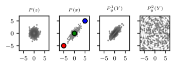
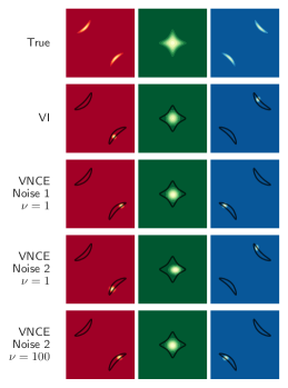
Figure 2 shows various posteriors over the latent space, conditioning on three colour-coded landmark ${\mathbf{x}}$ points marked in Figure 1. The first two rows show the true posterior, calculated with numerical integration, and the approximate posterior learned using standard VI. Approximate posteriors learned with VNCE are shown in the last three rows. The approximate posteriors learned with VNCE are similar to those learned with standard VI when either the noise is a good match to the data (row 3), or when $\nu$ is large (final row). In particular, the VNCE posteriors show the same low-variance, mode-seeking behaviour.

These connections between VNCE and standard VI are in line with Theorem 1 which states that as the ratio $\phi_{{\boldsymbol{\theta}}}({\mathbf{x}})/(\phi_{{\boldsymbol{\theta}}}({\mathbf{x}})+\nu p_{\mathbf{y}}({\mathbf{x}}))$ tends to $0$, VNCE minimises an f-divergence that approaches the standard KL. This ratio becomes closer to zero precisely when the noise assigns a higher probability to the data or when $\nu$ is large. Conversely, when the noise is ‘bad’ and $\nu$ in insufficiently large (penultimate row) VNCE produces approximate posteriors that are slightly distorted in comparison to standard VI.

Theorem 1 also states that the optimal $q$ obtained with VNCE is the true posterior. In this setting, it is not possible for $q$ to exactly recover the true posterior, since we have restricted $q$ to be Gaussian with no correlation structure. Still, we see that the approximate posteriors of both VI and VNCE are reasonable fits to the true posteriors, modulo parametric restrictions.

Figure 3: EM-type algorithm for VNCE. The figure reads row-by-row, from left to right. In the E-step, we set $q(z|x)$ equal to the true posterior $p(z|x;\theta_{t})$, making the VNCE objective tight at $\theta_{t}$. In the M-step we optimise $\theta$ using the VNCE objective, and hence the red dashed line shifts to the centre of the red square.

4.2 Parameter estimation with VNCE

The following simulations illustrate Theorem 2, which states that VNCE and NCE have the same maximum. We consider both a normalised and unnormalised mixture of two Gaussians (MoG).

Normalised mixture of Gaussians

The model is given by

$$p(x,z;\theta)=\frac{z}{2}\mathcal{N}(x;0,\sigma_{1}^{2})+\frac{(1-z)}{2}\mathcal{N}(x;0,\theta^{2}),$$ (24)

with $z\in\{0,1\}$ and $x\in\mathbb{R}$. We assume that the variance of the first component, $\sigma_{1}^{2}$, is known, and we estimate the value of $\theta$. For a simple experiment, we set $\sigma_{1}=1$ and let $\theta^{*}=4$ be the true value of $\theta$. We set the noise distribution to be $p_{\mathbf{y}}(y)=\mathcal{N}(y;0,{\theta^{*}}^{2})$. For the variational distribution, we can use the true posterior of the model,

$$p(z=0\ |\ x;\theta)=\frac{1}{1+\frac{\theta}{\sigma_{1}}\exp(\frac{-x^{2}}{2}(\frac{1}{\sigma_{1}^{2}}-\frac{1}{\theta^{2}}))},$$ (25)

enabling us to apply the EM type algorithm presented in Corollary 1.

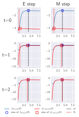
Figure 3 illustrates the results with plots of the NCE and VNCE objectives obtained after each E-step and M-step during learning. It is clear from the figure that the value of the NCE objective at the current parameter (red-dashed line) never decreases, in accordance with Corollary 1. Moreover, the figure validates Theorem 2, which states that the maximum of the VNCE objective with respect to $\theta$ and $q$ equals the maximum of the NCE objective with respect to $\theta$. We see this from the overlap of the blue circle (maximum of NCE) and the red square (maximum of VNCE) in the final plot (bottom-right).

Figure 4: Log sample size vs. log mean-squared error for the standard deviation and scaling parameter of 500 different unnormalised MoG models. Central lines show median MSEs over 500 runs, whilst dashed lines mark the 1st and 9th deciles. The negative slope of the red line in both plots is evidence of the consistency of VNCE.

Unnormalised mixture of Gaussians

An unnormalised version of the MoG model is given by

$$\phi(x,z;\theta,c)=e^{-c}\left(ze^{-\frac{x^{2}}{2\sigma_{1}^{2}}}+(1-z)e^{-\frac{x^{2}}{2\theta^{2}}}\right)$$ (26)

where $c$ is a scaling parameter.

Whilst we could proceed as before, using an EM algorithm with the true posterior, we will not have access to such a posterior for more complex models. Thus, we test the performance of VNCE when using an approximate variational distribution $q$, given by

$$q(z=0\ |\ x;\boldsymbol{w})=\frac{1}{1+\exp(w_{0}+w_{1}x+w_{2}x^{2})},$$ (27)

where $\boldsymbol{w}=(w_{0},w_{1},w_{2})^{\top}$ are the variational parameters. This $q$ family contains the true posterior.

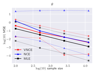
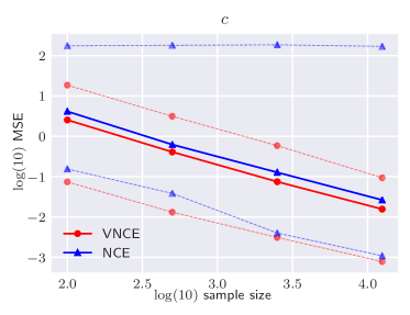
We test the accuracy of VNCE for parameter estimation using a 500-run population analysis over multiple sample sizes. NCE and maximum likelihood estimation (MLE) serve as baseline methods (after normalisation and/or summing over latent variables). For both NCE and VNCE, we used $\nu=1$ and the same Gaussian noise distribution as for the normalised MoG (for more details, see the supplementary material).

Figure 4 shows the mean square error (MSE) $\mathbb{E}||\theta-\theta^{*}||^{2}$ for VNCE, NCE and MLE. The left plot demonstrates that the estimation accuracy of VNCE increases with sample size, and is comparable to that of NCE. This gives evidence of the consistency of VNCE. Interestingly, NCE was much more prone to falling into local optima, despite multiple random initialisations, as shown by the blue upper dashed line.

5 Graphical model structure learning from incomplete data

We consider an important use-case of VNCE: the training of unnormalised models from incomplete data, treating missing values as latent variables. Specifically, we use VNCE to estimate the parameters of an undirected graphical model from incomplete data. This application is motivated by Lin et al., (2016), who used (non-negative) score matching (Hyvärinen,, 2007) for estimation. Unfortunately, latent variables cannot be handled within the score matching framework and so the missing values were either discarded or set to zero.

5.1 Model specification

The undirected graphical model is a truncated Gaussian given by

$$\phi({\mathbf{x}};{\mathbf{K}},c)=\exp\left(-\frac{1}{2}{\mathbf{x}}^{\top}{\mathbf{K}}{\mathbf{x}}-c\right){\mathbb{I}}({\mathbf{x}}\in A),$$ (28)

where $A$ is the support of $\phi$, which equals $[0,+\infty]^{d}$ in our experiments, and $c$ is a scaling parameter. The partition function of $\phi$ is intractable to compute, except in very low dimensions (Horrace,, 2005), rendering the model unnormalised.

The model in (28) defines an undirected graph where the variables correspond to nodes and where there is an edge between the nodes of $x_{i}$ and $x_{j}$ whenever the $(i,j)$-th element of ${\mathbf{K}}$ is non-zero. In such graphs, a missing edge between $x_{i}$ and $x_{j}$ means that they are conditionally independent given the remaining variables (see e.g. Koller and Friedman,, 2009).

We split each data point ${\mathbf{x}}_{i}=({\mathbf{x}}_{i}^{o},{\mathbf{x}}_{i}^{m})$ into its observed and missing components. We treat the (potentially empty) set of missing values ${\mathbf{x}}_{i}^{m}$ as latent variables, i.e. they correspond to the ${\mathbf{z}}$ variables used before. The true posterior over these missing variables, whilst also a truncated normal, is generally intractable to compute (Horrace,, 2005). We therefore use a log-normal variational family to approximate it.

A subtle but important technical point is that there are $2^{d}-1$ non-trivial patterns of missingness that can occur in the data, and so we need a variational posterior for each possible pattern. We achieve this by parametrising a joint lognormal distribution over all dimensions, since all of its conditionals are computable in closed-form.

Similarly, we require noise samples, ${\mathbf{y}}_{i}=({\mathbf{y}}_{i}^{o},{\mathbf{y}}_{i}^{m})$, that have the same pattern of missingness as the ${\mathbf{x}}_{i}$. In order to compute the probability of ${\mathbf{y}}_{i}^{o}$, we need a joint noise distribution for which we can compute all marginals. We achieve this by using a fully-factorised product of truncated normals. The parameters of each univariate truncated normal is estimated from the observed data for that dimension (see supplementary material).

5.2 Simulations

Figure 5: Left: ring-graph. Right: hub. Area under the ROC curve for increasing amounts of missing data. Larger AUC means better performance. Bars denote interquartile ranges for 10 runs, central markers medians.

We consider two types of ground-truth graphs, and thus matrices ${\mathbf{K}}$. The first is a ring-structured graph, where we obtain ${\mathbf{K}}$ from an initial matrix of all-zeros by first sampling each element of the superdiagonal from $\mathcal{U}(0.3,0.5)$, as well as the top-right hand corner, and then symmetrising. The second type of graph is an augmented version of the ring-graph, where we have added ‘hubs’, i.e. nodes with a high degree. We randomly select $1/10$ nodes to be connected to $1/4$ of all other nodes. In both cases, we set the diagonal elements to a common positive number that ensures ${\mathbf{K}}$ is diagonally dominant.

We simulate 10 datasets of $n=1000$ samples with $d=20$ dimensions using the Gibbs sampler from the tmvtnorm package in R with a burnin period of 100 samples and thinning factor of 10. For each dataset, we generate six more, by discarding a percentage $p$ of the $n\times d$ values at random, where $p$ ranges from $0\%$ to $50\%$ in increments of $10\%$.

We compare three methods: (i) VNCE, (ii) NCE with missing values filled-in with the observed mean for that dimension, and (iii) stochastic gradient ascent on the log-likelihood using the gradient in (3), with the expectations approximated via Monte Carlo sampling (MC-MLE). While VNCE and NCE were optimised with a standard optimiser (BFGS), for MC-MLE, one has to manually select suitable step-sizes for gradient ascent (for more details, see the supplementary material).

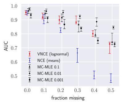
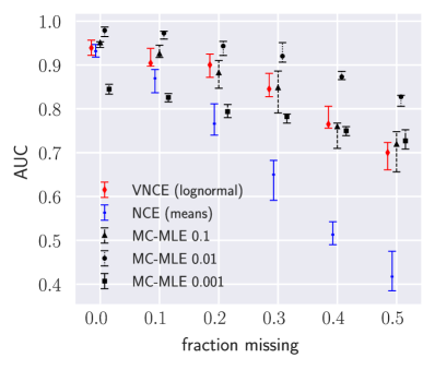
For each data set and method, we can extract a learned graph from the estimated ${\mathbf{K}}$ by applying a threshold. If an element of ${\mathbf{K}}$ is less than the threshold, the corresponding edge is not included in the graph. For various thresholds, we then compute a true-positive rate as the percentage of ground-truth edges we correctly identify. Similarly, we compute a false-positive rate. Jointly plotting the two rates yields an ROC curve, and we use the area under the ROC curve (AUC) as the performance metric.

Figure 5 shows the results for the ring-graph (left) and the graph with hubs (right). In both cases, we observe significant, and increasing, performance gains for VNCE over NCE (with mean imputation) as larger fractions of data are missing. This shows that inference of the missing values from the observed ones improves parameter estimation. The difference is particular stark when 40% or more data is missing, as NCE is hardly better than random guessing of edges (which corresponds to an AUC of 0.5).

With careful tuning of the learning rate, MC-MLE achieves the best performance of all three methods. This makes sense, since MLE is the gold-standard for parameter estimation. However, for other reasonable (but non-optimal) learning rates, VNCE performs comparably. This is an important finding for two reasons. Firstly, MC-MLE is not feasible for many models due to the lack of an efficient sampler, and so it is valuable to know that VNCE can serve as a reasonable replacement. Secondly, when modelling actual data, it is not obvious how to select the stepsize, and other hyperparameters, for MC-MLE, due to the lack of a tractable objective function. VNCE, in contrast, has a well-defined objective function that can be optimised with powerful optimisers. Moreover, it can be used for cross-validation in combination with regularisation.

6 Conclusions

We developed a new method for training unnormalised latent variable models that makes variational inference possible within the noise-contrastive framework. This contribution addresses an important gap in the literature, since few estimation methods exist for this highly-flexible, yet doubly-intractable, class of models.

We proved that variational noise-contrastive estimation (VNCE) can be used for both parameter estimation and posterior inference of latent variables. The proposed VNCE framework has the same level of generality as standard variational inference, meaning that advances made there can be directly imported to the unnormalised setting.

The theoretical results were validated on toy models and we demonstrated the effectiveness of VNCE on the realistic problem of graphical model structure learning with incomplete data. By working with a model for which sampling is tractable, we were able to assess VNCE in its ability to reach the likelihood-based solution. We found that VNCE performed well and that it is a promising option for estimating more complex unnormalised latent variables models where the sampling-based approaches become infeasible.

Acknowledgements

We would like to thank Iain Murray for feedback on preliminary versions of this text. Benjamin Rhodes was supported in part by the EPSRC Centre for Doctoral Training in Data Science, funded by the UK Engineering and Physical Sciences Research Council (grant EP/L016427/1) and the University of Edinburgh. This work has made use of the resources provided by the Edinburgh Compute and Data Facility (ECDF).

Appendix A Convexity result for NCE lower bound

For non-negative real numbers $a,b$ and $u$, the function

$$f(u)=\log(a+bu^{-1})$$ (29)

is convex. We see this by differentiating $f$ twice:

$$f^{\prime}(u)=-\frac{b}{au^{2}+bu}\hskip 19.91692ptf^{\prime\prime}(u)=\frac{b(2au+b)}{(au^{2}+bu)^{2}},$$ (30)

and observing that $f^{\prime\prime}(u)\geq 0$ since $a,b$ and $u$ are non-negative.

Appendix B Proof of Lemma 1

Key to this proof is the following factorisation

$$\phi_{{\boldsymbol{\theta}}}({\mathbf{x}},{\mathbf{z}})=\phi_{{\boldsymbol{\theta}}}({\mathbf{x}})p_{{\boldsymbol{\theta}}}({\mathbf{z}}\>|\>{\mathbf{x}}),$$ (31)

where the conditional distribution is normalised and the factorisation holds because the unnormalised distributions on either side of the equation have the same partition function

$$\int\int\phi_{{\boldsymbol{\theta}}}({\mathbf{x}},{\mathbf{z}})\operatorname{d\!}{\mathbf{z}}\operatorname{d\!}{\mathbf{x}}=\int\phi_{{\boldsymbol{\theta}}}({\mathbf{x}})\operatorname{d\!}{\mathbf{x}}.$$ (32)

With this factorisation at hand, we now consider the difference between the NCE objective: $J_{\scaleto{\mathrm{NCE}}{4pt}}({\boldsymbol{\theta}})$ in (4) and the VNCE objective: $J_{\scaleto{\mathrm{VNCE}}{4pt}}({\boldsymbol{\theta}},q)$ in (3.1). Each objective consists of two terms: the first is an expectation with respect to the data, the second an expectation with respect to the noise distribution $p_{\mathbf{y}}$. The second terms of $J_{\scaleto{\mathrm{NCE}}{4pt}}$ and $J_{\scaleto{\mathrm{VNCE}}{4pt}}$ are identical, so their difference equals the difference between their first terms

$$J_{\scaleto{\mathrm{NCE}}{4pt}}({\boldsymbol{\theta}})-J_{\scaleto{\mathrm{VNCE}}{4pt}}({\boldsymbol{\theta}},q)$$

$$=\mathbb{E}_{{\mathbf{x}}}\log\left(\frac{\phi_{{\boldsymbol{\theta}}}({\mathbf{x}})}{\phi_{{\boldsymbol{\theta}}}({\mathbf{x}})+\nu p_{\mathbf{y}}({\mathbf{x}})}\right)-\mathbb{E}_{{\mathbf{x}}}\mathbb{E}_{{\mathbf{z}}\sim q({\mathbf{z}}\>|\>{{\mathbf{x}}})}\log\left(\frac{\phi_{{\boldsymbol{\theta}}}({\mathbf{x}},{\mathbf{z}})}{\phi_{{\boldsymbol{\theta}}}({\mathbf{x}},{\mathbf{z}})+\nu p_{\mathbf{y}}({\mathbf{x}})q({\mathbf{z}}\>|\>{\mathbf{x}})}\right)$$ (33)

$$=\mathbb{E}_{{\mathbf{x}}}\mathbb{E}_{{\mathbf{z}}\sim q({\mathbf{z}}\>|\>{{\mathbf{x}}})}\biggl{[}\log\left(\frac{\phi_{{\boldsymbol{\theta}}}({\mathbf{x}})}{\phi_{{\boldsymbol{\theta}}}({\mathbf{x}})+\nu p_{\mathbf{y}}({\mathbf{x}})}\right)+\log\left(1+\frac{\nu p_{\mathbf{y}}({\mathbf{x}})q({\mathbf{z}}\>|\>{\mathbf{x}})}{\phi_{{\boldsymbol{\theta}}}({\mathbf{x}})p_{{\boldsymbol{\theta}}}({\mathbf{z}}\>|\>{\mathbf{x}})}\right)\biggr{]}$$ (34)

$$=\mathbb{E}_{{\mathbf{x}}}\mathbb{E}_{{\mathbf{z}}\sim q({\mathbf{z}}\>|\>{{\mathbf{x}}})}\left[\log\left(\frac{\phi_{{\boldsymbol{\theta}}}({\mathbf{x}})}{\phi_{{\boldsymbol{\theta}}}({\mathbf{x}})+\nu p_{\mathbf{y}}({\mathbf{x}})}+\frac{\phi_{{\boldsymbol{\theta}}}({\mathbf{x}})}{\phi_{{\boldsymbol{\theta}}}({\mathbf{x}})+\nu p_{\mathbf{y}}({\mathbf{x}})}\frac{\nu p_{\mathbf{y}}({\mathbf{x}})}{\phi_{{\boldsymbol{\theta}}}({\mathbf{x}})}\frac{q({\mathbf{z}}\>|\>{\mathbf{x}})}{p_{{\boldsymbol{\theta}}}({\mathbf{z}}\>|\>{\mathbf{x}})}\right)\right]$$ (35)

$$=\mathbb{E}_{{\mathbf{x}}}\mathbb{E}_{{\mathbf{z}}\sim q({\mathbf{z}}\>|\>{{\mathbf{x}}})}\left[\log\left(\frac{\phi_{{\boldsymbol{\theta}}}({\mathbf{x}})}{\phi_{{\boldsymbol{\theta}}}({\mathbf{x}})+\nu p_{\mathbf{y}}({\mathbf{x}})}+\frac{\nu p_{\mathbf{y}}({\mathbf{x}})}{\phi_{{\boldsymbol{\theta}}}({\mathbf{x}})+\nu p_{\mathbf{y}}({\mathbf{x}})}\frac{q({\mathbf{z}}\>|\>{\mathbf{x}})}{p_{{\boldsymbol{\theta}}}({\mathbf{z}}\>|\>{\mathbf{x}})}\right)\right]$$ (36)

$$=\mathbb{E}_{{\mathbf{x}}}\mathbb{E}_{{\mathbf{z}}\sim q({\mathbf{z}}\>|\>{{\mathbf{x}}})}\left[\log\left(\frac{\phi_{{\boldsymbol{\theta}}}({\mathbf{x}})}{\phi_{{\boldsymbol{\theta}}}({\mathbf{x}})+\nu p_{\mathbf{y}}({\mathbf{x}})}+\left(1-\frac{\phi_{{\boldsymbol{\theta}}}({\mathbf{x}})}{\phi_{{\boldsymbol{\theta}}}({\mathbf{x}})+\nu p_{\mathbf{y}}({\mathbf{x}})}\right)\frac{q({\mathbf{z}}\>|\>{\mathbf{x}})}{p_{{\boldsymbol{\theta}}}({\mathbf{z}}\>|\>{\mathbf{x}})}\right)\right]$$ (37)

$$=\mathbb{E}_{{\mathbf{x}}}\mathbb{E}_{{\mathbf{z}}\sim q({\mathbf{z}}\>|\>{{\mathbf{x}}})}\left[\log\left(\kappa_{{\mathbf{x}}}+(1-\kappa_{{\mathbf{x}}})\frac{q({\mathbf{z}}\>|\>{\mathbf{x}})}{p_{{\boldsymbol{\theta}}}({\mathbf{z}}\>|\>{\mathbf{x}})}\right)\right]$$ (38)

$$=\mathbb{E}_{{\mathbf{x}}}\left[D_{f_{{\mathbf{x}}}}(p_{{\boldsymbol{\theta}}}({\mathbf{z}}\>|\>{\mathbf{x}})\;\|\;q({\mathbf{z}}\>|\>{\mathbf{x}}))\right],$$ (39)

where $f_{{\mathbf{x}}}(u)=\log(\kappa_{{\mathbf{x}}}+(1-\kappa_{{\mathbf{x}}})u^{-1})$. To ensure that that $D_{f_{{\mathbf{x}}}}$ is a valid f-divergence, we need to prove that $f$ is convex and $f_{{\mathbf{x}}}(1)=0$. The latter is trivial, since $f_{{\mathbf{x}}}(1)=\log(\kappa_{{\mathbf{x}}}+(1-\kappa_{{\mathbf{x}}}))=\log(1)=0$, and convexity follows directly from Supplementary Materials A.

We now prove that this f-divergence can be expressed as the difference of two KL-divergences as in (17) in the main text. To do this, we pull $q/p$ outside of the log in (38),

$$D_{f_{{\mathbf{x}}}}(p_{{\boldsymbol{\theta}}}({\mathbf{z}}\>|\>{\mathbf{x}})\;\|\;q({\mathbf{z}}\>|\>{\mathbf{x}}))$$

$$=\mathbb{E}_{{\mathbf{z}}\sim q({\mathbf{z}}\>|\>{{\mathbf{x}}})}\left[\log\frac{q({\mathbf{z}}\>|\>{\mathbf{x}})}{p_{{\boldsymbol{\theta}}}({\mathbf{z}}\>|\>{\mathbf{x}})}\right]+\mathbb{E}_{{\mathbf{z}}\sim q({\mathbf{z}}\>|\>{{\mathbf{x}}})}\left[\log\left(\kappa_{{\mathbf{x}}}\frac{p_{{\boldsymbol{\theta}}}({\mathbf{z}}\>|\>{\mathbf{x}})}{q({\mathbf{z}}\>|\>{\mathbf{x}})}+(1-\kappa_{{\mathbf{x}}})\right)\right]$$ (40)

$$=\mathbb{E}_{{\mathbf{z}}\sim q({\mathbf{z}}\>|\>{{\mathbf{x}}})}\left[\log\frac{q({\mathbf{z}}\>|\>{\mathbf{x}})}{p_{{\boldsymbol{\theta}}}({\mathbf{z}}\>|\>{\mathbf{x}})}\right]-\mathbb{E}_{{\mathbf{z}}\sim q({\mathbf{z}}\>|\>{{\mathbf{x}}})}\left[\log\left(\frac{q({\mathbf{z}}\>|\>{\mathbf{x}})}{\kappa_{{\mathbf{x}}}p_{{\boldsymbol{\theta}}}({\mathbf{z}}\>|\>{\mathbf{x}})+(1-\kappa_{{\mathbf{x}}})q({\mathbf{z}}\>|\>{\mathbf{x}})}\right)\right]$$ (41)

$$=D_{KL}(q({\mathbf{z}}\>|\>{\mathbf{x}})\;\|\;p_{{\boldsymbol{\theta}}}({\mathbf{z}}\>|\>{\mathbf{x}}))-D_{KL}(q({\mathbf{z}}\>|\>{\mathbf{x}})\;\|\;m_{{\boldsymbol{\theta}}}({\mathbf{z}},{\mathbf{x}})).$$ (42)

where $m_{{\boldsymbol{\theta}}}({\mathbf{z}},{\mathbf{x}})=\kappa_{{\mathbf{x}}}p_{{\boldsymbol{\theta}}}({\mathbf{z}}\>|\>{\mathbf{x}})+(1-\kappa_{{\mathbf{x}}})q({\mathbf{z}}\>|\>{\mathbf{x}})$.

Appendix C Proof of Theorem 1

We first show that

$$J_{\scaleto{\mathrm{NCE}}{4pt}}({\boldsymbol{\theta}})=J_{\scaleto{\mathrm{VNCE}}{4pt}}({\boldsymbol{\theta}},q)\hskip 5.69054pt\Leftrightarrow\hskip 5.69054ptq({\mathbf{z}}\>|\>{\mathbf{x}})=p_{{\boldsymbol{\theta}}}({\mathbf{z}}\>|\>{\mathbf{x}}).$$ (43)

We could obtain this result directly from the lower bound in Section 3.1 in the main text. However, for brevity, we make use of the Lemma 1, where we obtained the equality

$$J_{\scaleto{\mathrm{NCE}}{4pt}}({\boldsymbol{\theta}})-J_{\scaleto{\mathrm{VNCE}}{4pt}}({\boldsymbol{\theta}},q)=\mathbb{E}_{{\mathbf{x}}}\left[D_{f_{{\mathbf{x}}}}(p_{{\boldsymbol{\theta}}}({\mathbf{z}}\>|\>{\mathbf{x}})\;\|\;q({\mathbf{z}}\>|\>{\mathbf{x}}))\right].$$ (44)

The f-divergence on the right-hand side is non-negative and equal to zero if and only if the two posteriors coincide. Hence, $J_{\scaleto{\mathrm{NCE}}{4pt}}({\boldsymbol{\theta}})=J_{\scaleto{\mathrm{VNCE}}{4pt}}({\boldsymbol{\theta}},q)$ if and only if $q({\mathbf{z}}\>|\>{\mathbf{x}})=p_{{\boldsymbol{\theta}}}({\mathbf{z}}\>|\>{\mathbf{x}})$.

We now show that

$$D_{f_{{\mathbf{x}}}}(p_{{\boldsymbol{\theta}}}({\mathbf{z}}\>|\>{\mathbf{x}})\;\|\;q({\mathbf{z}}\>|\>{\mathbf{x}}))\ \rightarrow\ D_{KL}(q({\mathbf{z}}\>|\>{\mathbf{x}})\;\|\;p_{{\boldsymbol{\theta}}}({\mathbf{z}}\>|\>{\mathbf{x}}))$$ (45)

as $\kappa_{{\mathbf{x}}}=\phi_{{\boldsymbol{\theta}}}({\mathbf{x}})/(\phi_{{\boldsymbol{\theta}}}({\mathbf{x}})+\nu p_{\mathbf{y}}({\mathbf{x}}))\rightarrow 0$. Again, this follows quickly from Lemma 1. Specifically, in (38), we obtained

$$J_{\scaleto{\mathrm{NCE}}{4pt}}({\boldsymbol{\theta}})-J_{\scaleto{\mathrm{VNCE}}{4pt}}({\boldsymbol{\theta}},q)=\mathbb{E}_{{\mathbf{z}}\sim q({\mathbf{z}}\>|\>{{\mathbf{x}}})}\left[\log\left(\kappa_{{\mathbf{x}}}+(1-\kappa_{{\mathbf{x}}})\frac{q({\mathbf{z}}\>|\>{\mathbf{x}})}{p_{{\boldsymbol{\theta}}}({\mathbf{z}}\>|\>{\mathbf{x}})}\right)\right].$$ (46)

As $\kappa_{{\mathbf{x}}}\rightarrow 0$, we obtain the standard KL-divergence.

Appendix D Proof of Theorem 2

Our goal is to show that

$$\max_{{\boldsymbol{\theta}}}J_{\scaleto{\mathrm{NCE}}{4pt}}({\boldsymbol{\theta}})=\max_{{\boldsymbol{\theta}}}\max_{q}J_{\scaleto{\mathrm{VNCE}}{4pt}}({\boldsymbol{\theta}},q).$$ (47)

We know from Theorem 1 that:

$$p_{{\boldsymbol{\theta}}}({\mathbf{z}}\>|\>{\mathbf{x}})=\underset{q}{\operatorname{arg}\,\operatorname{max}}\;J_{\scaleto{\mathrm{VNCE}}{4pt}}({\boldsymbol{\theta}},q),$$ (48)

and that, plugging this optimal $q$ into $J_{\scaleto{\mathrm{VNCE}}{4pt}}$ makes the variational lower bound tight,

$$J_{\scaleto{\mathrm{VNCE}}{4pt}}({\boldsymbol{\theta}},p_{{\boldsymbol{\theta}}}({\mathbf{z}}\>|\>{\mathbf{x}}))=J_{\scaleto{\mathrm{NCE}}{4pt}}({\boldsymbol{\theta}}).$$ (49)

Hence,

$$\max_{{\boldsymbol{\theta}}}\max_{q}J_{\scaleto{\mathrm{VNCE}}{4pt}}({\boldsymbol{\theta}},q)=\max_{{\boldsymbol{\theta}}}J_{\scaleto{\mathrm{VNCE}}{4pt}}({\boldsymbol{\theta}},p_{{\boldsymbol{\theta}}}({\mathbf{z}}\>|\>{\mathbf{x}}))=\max_{{\boldsymbol{\theta}}}J_{\scaleto{\mathrm{NCE}}{4pt}}({\boldsymbol{\theta}}).$$ (50)

Appendix E Proof of Corollary 1

Let $k\in\mathbb{N}$. After the E-step of optimisation, we have $q_{k}({\mathbf{z}}\>|\>{\mathbf{x}})=p({\mathbf{z}}\>|\>{\mathbf{x}};{\boldsymbol{\theta}}_{k})$ and so, by Lemma 1,

$$J_{\scaleto{\mathrm{NCE}}{4pt}}({\boldsymbol{\theta}}_{k})-J_{\scaleto{\mathrm{VNCE}}{4pt}}({\boldsymbol{\theta}}_{k},q_{k})=\mathbb{E}_{{\mathbf{x}}}\left[D_{f_{{\mathbf{x}}}}(p({\mathbf{z}}\>|\>{\mathbf{x}};{\boldsymbol{\theta}}_{k})\;\|\;p({\mathbf{z}}\>|\>{\mathbf{x}};{\boldsymbol{\theta}}_{k}))\right]=0,$$ (51)

implying that $J_{\scaleto{\mathrm{VNCE}}{4pt}}({\boldsymbol{\theta}}_{k},q_{k})=J_{\scaleto{\mathrm{NCE}}{4pt}}({\boldsymbol{\theta}}_{k})$. Now, in the M-step of optimisation, we have

$${\boldsymbol{\theta}}_{k+1}=\underset{{\boldsymbol{\theta}}}{\operatorname{arg}\,\operatorname{max}}\;J_{\scaleto{\mathrm{VNCE}}{4pt}}({\boldsymbol{\theta}},q_{k})\ \ \Longrightarrow\ \ J_{\scaleto{\mathrm{VNCE}}{4pt}}({\boldsymbol{\theta}}_{k+1},q_{k})\geq J_{\scaleto{\mathrm{VNCE}}{4pt}}({\boldsymbol{\theta}}_{k},q_{k})\ ,$$ (52)

finally, by using Lemma 1 again, we see that $J_{\scaleto{\mathrm{NCE}}{4pt}}({\boldsymbol{\theta}}_{k+1})\geq J_{\scaleto{\mathrm{VNCE}}{4pt}}({\boldsymbol{\theta}}_{k+1},q_{k})$. Putting everything together,

$$J_{\scaleto{\mathrm{NCE}}{4pt}}({\boldsymbol{\theta}}_{k+1})\geq J_{\scaleto{\mathrm{VNCE}}{4pt}}({\boldsymbol{\theta}}_{k+1},q_{k})\geq J_{\scaleto{\mathrm{VNCE}}{4pt}}({\boldsymbol{\theta}}_{k},q_{k})=J_{\scaleto{\mathrm{NCE}}{4pt}}({\boldsymbol{\theta}}_{k})\ .$$ (53)

Appendix F Optimal proposal distribution in the second term of the VNCE objective

We know from Theorem 1 that the optimal variational distribution is the true posterior, $q({\mathbf{z}}\>|\>{\mathbf{y}})=p({\mathbf{z}}\>|\>{\mathbf{y}};{\boldsymbol{\theta}})$. Thus, we simply need to show that the true posterior is the optimal proposal distribution for the importance sampling (IS) estimate in the second term of the VNCE objective.

As shown in Supplementary Materials B, the following factorisation holds

$$\phi_{{\boldsymbol{\theta}}}({\mathbf{y}},{\mathbf{z}})=\phi_{{\boldsymbol{\theta}}}({\mathbf{y}})p_{{\boldsymbol{\theta}}}({\mathbf{z}}\>|\>{\mathbf{y}}).$$ (54)

Using this factorisation of $\phi$, we get

$$\phi({\mathbf{y}};{\boldsymbol{\theta}}) =\mathbb{E}_{{\mathbf{z}}\sim q({\mathbf{z}}\>|\>{\mathbf{y}})}\left[\frac{\phi({\mathbf{y}},{\mathbf{z}};{\boldsymbol{\theta}})}{q({\mathbf{z}}\>|\>{\mathbf{y}})}\right]$$ (55)

$$=\phi({\mathbf{y}};{\boldsymbol{\theta}})\mathbb{E}_{{\mathbf{z}}\sim q({\mathbf{z}}\>|\>{\mathbf{y}})}\left[\frac{p({\mathbf{z}}\>|\>{\mathbf{y}};{\boldsymbol{\theta}})}{q({\mathbf{z}}\>|\>{\mathbf{y}})}\right].$$ (56)

Hence, the variance of a Monte Carlo estimate of the expectation in (55) will equal the variance of a Monte Carlo estimate of the expectation in (56). When $q({\mathbf{z}}\>|\>{\mathbf{y}})=p({\mathbf{z}}\>|\>{\mathbf{y}};{\boldsymbol{\theta}})$, the latter expectation equals one, yielding a zero-variance—and thus optimal—Monte Carlo estimate.

We have therefore shown that the use of IS is optimal when we have access to $p({\mathbf{z}}\>|\>{\mathbf{y}};{\boldsymbol{\theta}})$. More generally, it will still be sensible when we have access to a parameterised approximate posterior $q({\mathbf{z}}\>|\>{\mathbf{y}};{\boldsymbol{\alpha}})$, which is close to the true posterior. However, one potential issue that could arise in practice is that $q$ is only close to the true posterior when conditioning on data ${\mathbf{x}}$, but not when conditioning on noise samples ${\mathbf{y}}$. This is because we only optimise the parameters of $q$ with respect to the first term of the VNCE objective, in which we only condition on data ${\mathbf{x}}$. In our experiments, we did not observe such an issue. However, we expect that if ${\mathbf{z}}$ is high-dimensional and the noise distribution is sufficiently different from the data distribution, then this could become an issue.

Appendix G Experimental settings for toy approximate inference problem

In Section 4.1 we approximated a posterior $p({\mathbf{z}}\>|\>{\mathbf{x}})$ with a variational distribution $q({\mathbf{z}}\>|\>{\mathbf{x}};{\boldsymbol{\alpha}})=\mathcal{N}({\mathbf{z}};\ \boldsymbol{\mu}({\mathbf{x}};{\boldsymbol{\alpha}}),\boldsymbol{\Sigma}({\mathbf{x}};{\boldsymbol{\alpha}}))$, where $\boldsymbol{\Sigma}$ is a diagonal covariance matrix, and $\boldsymbol{\mu}$ and $\boldsymbol{\Sigma}$ are parametrised by a single 2-layer feed-forward neural network with weights ${\boldsymbol{\alpha}}$.

The output layer of the neural network has 4 dimensions, containing the concatenated vectors $\boldsymbol{\mu}$ and $\log(\mathrm{diag}(\boldsymbol{\Sigma}))$. The input to the network is a 2 dimensional vector ${\mathbf{x}}$ of observed data. In each hidden layer there are 100 hidden units, generated by an affine mapping composed with a $\tanh$ non-linearity applied to the previous layer. The weights of the network are initialised from $\mathcal{U}(-0.05,0.05)$ and optimised with stochastic gradient ascent in minibatches of $100$ and learning rate of $0.0001$ for a total of $50$ epochs.

Appendix H Experimental settings for toy parameter estimation (Figure 4)

Figure 4 shows the accuracy of VNCE for parameter estimation using a population analysis over multiple sample sizes, comparing to NCE and MLE. To produce it, we generated 500 distinct ground-truth values for the standard deviation parameter in the unnormalised MoG, sampling uniformly from the interval $[2,6]$. For each of the 500 sampled values of $\theta^{*}$, we estimate $\theta$ using all three estimation methods and with a range of sample sizes. Every run was initialised from five random values and the best result out of the five was kept in order to avoid local optima which exist since both the likelihood and NCE objective functions are bi-modal.

Appendix I Estimation of noise distribution for undirected graphical model experiments

Assume the observed data are organised in a matrix $X$ with each column containing all observations of a single variable. We want to fit a univariate truncated Gaussian to each column. To do so, we could estimate the means $\mu_{i}$ and variances $\sigma_{i}^{2}$ of the pre-truncated Gaussians using the following equations (Burkardt,, 2014), where $x_{i}$ denotes a column of $X$ with empirical mean $\bar{\mu}_{i}$ and variance $\bar{\sigma}_{i}^{2}$:

$$\bar{\mu_{i}} =\mu_{i}+\frac{\psi(\alpha)}{1-\Phi(\alpha)}\sigma_{i}, \bar{\sigma_{i}^{2}} =\left[1+\frac{\alpha\psi(\alpha)}{1-\Phi(\alpha)}-\left(\frac{\psi(\alpha)}{1-\Phi(\alpha)}\right)^{2}\right]\sigma_{i}^{2},$$ (57)

where $\psi$ is the pdf of a standard normal and $\Phi$ is its cdf. These pairs on non-linear simultaneous equations can then be solved with a variety of methods, such as Newton-Krylov (Knoll and Keyes,, 2004). However, whenever $\alpha=\frac{-\mu_{i}}{\sigma_{i}}\gg 0$, computing the fractions $\frac{\alpha\psi(\alpha)}{1-\Phi(\alpha)}$ , $\frac{\psi(\alpha)}{1-\Phi(\alpha)}$ becomes numerically unstable. In a short note available on GitHub, Fernandez-de-cossio Diaz, (2018) explains how to fix this using the more numerically stable scaled complementary error function $\operatorname{erfcx}(x)=\exp(x^{2})\operatorname{erf}(x)$, where $\operatorname{erf}(x)$ is the error function. Introducing the notation

$$F_{1}(x)=\frac{1}{\operatorname{erfcx}(x)},\hskip 28.45274ptF_{2}(x)=\frac{x}{\operatorname{erfcx}(x)},$$ (58)

we can then re-express the required fractions in a numerically stable form,

$$\frac{\alpha\psi(\alpha)}{1-\Phi(\alpha)} =\frac{2}{\sqrt{\pi}}F_{2}(\frac{\alpha}{\sqrt{2}}), \frac{\psi(\alpha)}{1-\Phi(\alpha)} =\frac{2}{\sqrt{\pi}}F_{2}(\frac{\alpha}{\sqrt{2}})-\frac{2}{\pi}\left[F_{1}(\frac{\alpha}{\sqrt{2}})\right]^{2}.$$ (59)

Appendix J Experimental settings for the undirected graphical model experiments

For VNCE and NCE we set $\nu=10$, and optimise with the BFGS optimisation method of Python’s scipy.optimize.minimize, capping the number of iterations at 80. In the case of VNCE, we use variational-EM, alternating every 5 iterations, and approximating expectations with respect to the variational distribution with $5$ samples per datapoint. Derivatives with respect to the variational parameters are computed using the reparametrisation trick (Kingma and Welling,, 2013; Rezende et al.,, 2014), using a standard normal as the base distribution.

For MC-MLE, we apply stochastic gradient ascent for 80 epochs with minibatches of 100 datapoints. The Monte-Carlo expectations with respect to the posterior distribution and joint distribution use 5 samples per datapoint. These samples are obtained with the tmvtnorm Gibbs sampler, using the Gibbs sampler from the tmvtnorm package in R with a burnin period of 100 samples and thinning factor of 10.

For VNCE and NCE, we do not enforce positive semi-definiteness of the matrix ${\mathbf{K}}$ in (28), in line with Lin et al., (2016). For MCMLE, we do enforce it, since tmvtnorm requires it.

Bibliography

- Barber, (2012) Barber, D. (2012). Bayesian reasoning and machine learning. Cambridge University Press.
- Barthelmé and Chopin, (2015) Barthelmé, S. and Chopin, N. (2015). The Poisson transform for unnormalised statistical models. Statistics and Computing, 25(4):767–780.
- Belanger and McCallum, (2016) Belanger, D. and McCallum, A. (2016). Structured prediction energy networks. In International Conference on Machine Learning, pages 983–992.
- Burkardt, (2014) Burkardt, J. (2014). The truncated normal distribution. Department of Scientific Computing Website, Florida State University.
- Ceylan and Gutmann, (2018) Ceylan, C. and Gutmann, M. U. (2018). Conditional Noise-Contrastive Estimation of Unnormalised Models. Proceedings of the 35th International Conference on Machine Learning.
- Dempster et al., (1977) Dempster, A. P., Laird, N. M., and Rubin, D. B. (1977). Maximum likelihood from incomplete data via the EM algorithm. Journal of the Royal Statistical Society. Series B (methodological), pages 1–38.
- Fernandez-de-cossio Diaz, (2018) Fernandez-de-cossio Diaz, J. (2018). Moments of the univariate truncated normal distribution.
- Gutmann and Hirayama, (2011) Gutmann, M. and Hirayama, J. (2011). Bregman divergence as general framework to estimate unnormalized statistical models. In Proceedings of the Conference on Uncertainty in Artificial Intelligence (UAI).
- Gutmann and Hyvärinen, (2012) Gutmann, M. and Hyvärinen, A. (2012). Noise-contrastive estimation of unnormalized statistical models, with applications to natural image statistics. Journal of Machine Learning Research, 13:307–361.
- Hinton, (2002) Hinton, G. E. (2002). Training products of experts by minimizing contrastive divergence. Neural Computation, 14(8).
- Hoffman et al., (2013) Hoffman, M. D., Blei, D. M., Wang, C., and Paisley, J. (2013). Stochastic variational inference. The Journal of Machine Learning Research, 14(1):1303–1347.
- Horrace, (2005) Horrace, W. C. (2005). Some results on the multivariate truncated normal distribution. Journal of Multivariate Analysis, 94(1):209–221.
- Huang et al., (2015) Huang, W., Wu, Z., Liang, C., Mitra, P., and Giles, C. L. (2015). A neural probabilistic model for context based citation recommendation. In Twenty-Ninth AAAI Conference on Artificial Intelligence.
- Hyvärinen, (2005) Hyvärinen, A. (2005). Estimation of non-normalized statistical models by score matching. Journal of Machine Learning Research, 6(Apr):695–709.
- Hyvärinen, (2007) Hyvärinen, A. (2007). Some extensions of score matching. Computational statistics & data analysis, 51(5):2499–2512.
- Jordan et al., (1999) Jordan, M. I., Ghahramani, Z., Jaakkola, T. S., and Saul, L. K. (1999). An introduction to variational methods for graphical models. Machine learning, 37(2):183–233.
- Kim et al., (2018) Kim, Y., Wiseman, S., and Rush, A. M. (2018). A tutorial on deep latent variable models of natural language. arXiv preprint arXiv:1812.06834.
- Kingma et al., (2014) Kingma, D. P., Mohamed, S., Rezende, D. J., and Welling, M. (2014). Semi-supervised learning with deep generative models. In Advances in Neural Information Processing Systems, pages 3581–3589.
- Kingma and Welling, (2013) Kingma, D. P. and Welling, M. (2013). Stochastic gradient VB and the variational auto-encoder. The 2nd International Conference on Learning Representations.
- Knoll and Keyes, (2004) Knoll, D. A. and Keyes, D. E. (2004). Jacobian-free Newton–Krylov methods: a survey of approaches and applications. Journal of Computational Physics, 193(2):357–397.
- Koller and Friedman, (2009) Koller, D. and Friedman, N. (2009). Probabilistic Graphical Models. MIT Press.
- Lin et al., (2016) Lin, L., Drton, M., and Shojaie, A. (2016). Estimation of high-dimensional graphical models using regularized score matching. Electronic journal of statistics, 10(1):806.
- Matsuda and Hyvarinen, (2018) Matsuda, T. and Hyvarinen, A. (2018). Estimation of Non-Normalized Mixture Models and Clustering Using Deep Representation. arXiv preprint arXiv:1805.07516.
- Mikolov et al., (2013) Mikolov, T., Sutskever, I., Chen, K., Corrado, G. S., and Dean, J. (2013). Distributed representations of words and phrases and their compositionality. In Advances in neural information processing systems, pages 3111–3119.
- Mnih and Gregor, (2014) Mnih, A. and Gregor, K. (2014). Neural variational inference and learning in belief networks. Proceedings of the 31st International Conference on Machine Learning.
- Mnih and Kavukcuoglu, (2013) Mnih, A. and Kavukcuoglu, K. (2013). Learning word embeddings efficiently with noise-contrastive estimation. In Advances in neural information processing systems, pages 2265–2273.
- Mnih and Whye, (2012) Mnih, A. and Whye, T. Y. (2012). A fast and simple algorithm for training neural probabilistic language models. In ICML.
- Nazabal et al., (2018) Nazabal, A., Olmos, P. M., Ghahramani, Z., and Valera, I. (2018). Handling incomplete heterogeneous data using VAEs. arXiv preprint arXiv:1807.03653.
- Oord et al., (2018) Oord, A. v. d., Li, Y., and Vinyals, O. (2018). Representation learning with contrastive predictive coding. arXiv preprint arXiv:1807.03748.
- Paisley et al., (2012) Paisley, J., Blei, D., and Jordan, M. (2012). Variational Bayesian inference with stochastic search. Proceedings of the 28th international conference on Machine learning.
- Pihlaja et al., (2010) Pihlaja, M., Gutmann, M., and Hyvärinen, A. (2010). A family of computationally efficient and simple estimators for unnormalized statistical models. In Proceedings of the Conference on Uncertainty in Artificial Intelligence (UAI).
- Ranganath et al., (2014) Ranganath, R., Gerrish, S., and Blei, D. (2014). Black box variational inference. In Artificial Intelligence and Statistics, pages 814–822.
- Rezende et al., (2014) Rezende, D. J., Mohamed, S., and Wierstra, D. (2014). Stochastic backpropagation and approximate inference in deep generative models. Proceedings of the 31st International Conference on Machine Learning.
- Riou-Durand and Chopin, (2018) Riou-Durand, L. and Chopin, N. (2018). Noise contrastive estimation: asymptotics, comparison with MC-MLE. arXiv:1801.10381 [math.ST].
- Ruslan and Hinton, (2009) Ruslan, S. and Hinton, G. (2009). Deep Boltzmann machines. J Mach Learn Res, 24(5):448–455.
- Tieleman and Hinton, (2009) Tieleman, T. and Hinton, G. (2009). Using fast weights to improve persistent contrastive divergence. In Proceedings of the 26th Annual International Conference on Machine Learning, pages 1033–1040. ACM.
- Younes, (1998) Younes, L. (1998). Stochastic gradient estimation strategies for Markov random fields. In Bayesian inference for inverse problems, volume 3459, pages 315–326. International Society for Optics and Photonics.
- Zhang et al., (2016) Zhang, W., Paquet, U., and Hofmann, K. (2016). Collective noise contrastive estimation for policy transfer learning. In Thirtieth AAAI Conference on Artificial Intelligence.