Tracking Influential Nodes in Time-Decaying Dynamic Interaction Networks

Abstract

Identifying influential nodes that can jointly trigger the maximum influence spread in networks is a fundamental problem in many applications such as viral marketing, online advertising, and disease control. Most existing studies assume that social influence is static and they fail to capture the dynamics of influence in reality. In this work, we address the dynamic influence challenge by designing efficient streaming methods that can identify influential nodes from highly dynamic node interaction streams. We first propose a general time-decaying dynamic interaction network (TDN) model to model node interaction streams with the ability to smoothly discard outdated data. Based on the TDN model, we design three algorithms, i.e., SieveADN, BasicReduction, and HistApprox. SieveADN identifies influential nodes from a special kind of TDNs with efficiency. BasicReduction uses SieveADN as a basic building block to identify influential nodes from general TDNs. HistApprox significantly improves the efficiency of BasicReduction. More importantly, we theoretically show that all three algorithms enjoy constant factor approximation guarantees. Experiments conducted on various real interaction datasets demonstrate that our approach finds near-optimal solutions with speed at least $5$ to $15$ times faster than baseline methods.

I Introduction

Online social networks allow their users to connect and interact with each other such as one user re-tweets/re-shares another user’s tweets/posts on Twitter/Facebook. Interactions between connected users can cause members in the network to be influenced. For example, a video goes viral on Twitter after being re-tweeted many times, a rumor spreads like a wildfire on Facebook via re-sharing, etc. In these scenarios, users in the network are influenced (i.e., they watched the video or got the rumor) via a cascade of user interactions. Understanding and leveraging social influence have been hot in both academia and business. For example, in academia, identifying $k$ users who can jointly trigger the maximum influence spread in a network is known as the influence maximization (IM) problem [1]; in business, leveraging social influence to boost product sales is known as viral marketing.

Figure 1: Observed node interactions (“$u$ RT @$v$ …” denotes that user $u$ re-tweeted user $v$’s tweet) and hidden evolving influence network (a directed edge $(u,v)$ denotes that $u$ influenced $v$). Influential nodes also evolve.

User interactions are first-hand evidences reflecting one user’s influence on another, e.g., user $a$ re-tweeting user $b$’s tweet implies that $b$ influenced $a$. Most studies on social influence [1, 2, 3, 4, 5, 6, 7, 8, 9] need to estimate influence probabilities based on observed user interactions [10, 11, 12]. Then, user influence is evaluated on an influence network, which is a directed graph with influence probabilities among nodes.

Dynamic influence challenge. One major issue in these studies is that both influence probabilities and influence network are assumed to be static, i.e., social influence is assumed to be static. However, social influence in real-world could be dynamic driven by the highly dynamic user interactions. For instance, user $a$ frequently re-tweeted user $b$’s tweets in the past few weeks, but stopped re-tweeting recently because $b$ posted offensive content and $a$ unfollowed $b$, thereby $b$ no longer exerting influence on $a$. Indeed, [13] reported that Twitter network is highly dynamic with about $9\%$ of all connections changing in every month. Moreover, user interactions can be drastically affected by external out-of-network sources such as mass media, newspapers, and TV stations [14]. Consequently, it is no longer suitable to assume that social influence is static; otherwise the identified influential users in IM may just quickly become outdated. This raises the following problem: in a world with highly dynamic user interactions, how can we efficiently identify $k$ most influential users at any time, as illustrated in Fig. 1?

A straightforward way to handle the dynamics of influence is that we re-compute everything from scratch every time we need to query influential users, i.e., re-estimate influence probabilities and re-identify influential users on the updated influence network. Obviously, this approach incurs too much computational overhead which may be unaffordable if we need to query influential users frequently. There have been some recent research efforts trying to address the dynamic influence challenge, such as the heuristic approaches [15, 16], building updatable sketches [17, 18], and the interchange greedy approach [19]. However, these methods either do not have theoretical guarantees on the quality of selected users (e.g., heuristic approaches [15, 16]), or they cannot handle highly dynamic data (e.g., the interchange greedy approach [19] actually degrades to the re-computation approach when influential users change significantly over time). In addition, these methods assume that influence probabilities are given in advance; however, estimating influence probabilities itself could be a high complexity inference task [10, 11, 20, 12], especially when influence probabilities are time-varying.

Present work: a streaming optimization approach. In this work, we explore the potential of designing efficient streaming methods to address the dynamic influence challenge.

When user interactions are continuously generated and aggregated in chronological order, they form a stream. An appealing approach for identifying influential users is to process this user interaction stream directly, in a streaming fashion [21]. Specifically, we attempt to maintain some compact intermediate results while processing the stream. We keep updating these intermediate results when new user interactions are examined. At any query time, we can quickly obtain a solution using the maintained intermediate results. This streaming approach has the potential to allow us to track influential users over time continuously. However, to materialize this ideal streaming approach, we need to carefully address following concerns.

• Data recency. Older user interactions are less significant than more recent ones in evaluating users’ current influence. For example, the observation that user $b$’s tweet was re-tweeted a year ago, is less valuable than the observation that $b$’s tweet was re-tweeted yesterday, when evaluating $b$’s current influence. The streaming approach is required to have a mechanism that can properly discard outdated data.

• Space and update efficiency. Space used by storing intermediate results should be compact and upper bounded with the progression of the stream. Meanwhile, the update operation should be as efficient as possible so that we can handle high-speed user interaction streams which are common in practice.

• Solution quality. The output solution should be close to the optimal solution at any query time.

This paper is essentially devoted to address above concerns by proposing a general streaming model and designing a set of streaming algorithms.

To address the data recency concern, a commonly used streaming model in the literature is the sliding-window model [22, 23, 24] where only the most recent $W$ elements in the stream remain active and the rest are discarded. For example, [25] recently developed a streaming method based on the sliding-window model to solve IM in a streaming fashion. However, the sliding-window model has its limitation which can be exposed by the following example.

Example 1.

Suppose we want to identify influential users on Twitter based on re-tweeting interactions, i.e., if a user’s tweets were re-tweeted by many other users, the user is considered to be influential. Alice is an influential user on Twitter for many years. Recently, Alice is ill and has been in hospital for weeks. During this period, Alice cannot use Twitter. Because Alice disappeared from her followers’ timelines, no user re-tweeted her tweets during this period.

In Example 1, if the sliding-window size is too small that no re-tweeting interaction related to Alice is observed, then Alice will be considered not influential, even though she has been influential for many years and her absence is merely temporal. This example demonstrates that sliding-window model does not discard outdated data in a smooth manner and results in unstable solutions. It thus motivates us to find better models.

• TDN model. In this work, we propose a general time-decaying dynamic interaction network (TDN) model to enable smoothly discarding outdated user interactions, rather than the non-smooth manner in sliding-window model. In TDN, each user interaction is assigned a lifetime. The lifetime is the maximum time span that a user interaction can remain active. Lifetime automatically decreases as time elapses. If the lifetime becomes zero, the corresponding user interaction is discarded. By choosing different lifetime assignments, TDN model can be configured to discard outdated user interactions in various ways, which include the sliding-window model as a special case. In short, TDN is a general streaming model to address the data recency issue.

• Efficient streaming algorithms. We address the other concerns by designing three streaming algorithms, i.e., SieveADN, BasicReduction, and HistApprox, all based on the TDN model. SieveADN can identify influential nodes over a special kind of TDNs. BasicReduction leverages SieveADN as a basic building block to identify influential nodes over general TDNs. HistApprox significantly improves the efficiency of BasicReduction. Our streaming algorithms are inspired by the streaming submodular optimization (SSO) techniques [26, 24]. Current SSO techniques can only handle insertion-only [26] and sliding-window [24] streams. To the best of our knowledge, the work in this paper is the first to handle more general time-decaying streams. More importantly, we theoretically show that our approach can find near-optimal solutions with both time and space efficiency.

Contributions. In summary, our contributions are as follows:

• We propose a general TDN model to model user interaction streaming data with the ability to discard outdated user interactions smoothly (§ II).

• We design three streaming algorithms based on the TDN model, namely SieveADN, BasicReduction, and HistApprox. Our algorithms are applicable to time-decaying streams and achieve a constant $(1/2-\epsilon)$ approximation guarantee (§ III and § IV).

• We conduct extensive experiments on various real interaction datasets. The results demonstrate that our approach outputs near-optimal solutions with speed at least $5$ to $15$ times faster than baseline methods. (§ V).

II Preliminaries and Problem Formulation

Notice that interactions are not necessarily occurred between two users but could be between any two entities, or nodes in networks. In this section, we first formally define the general node interaction data. Then we propose a time-decaying dynamic interaction network model. Finally, we formulate the problem of tracking influential nodes.

II-A Node Interactions

Definition 1 (Interaction).

An interaction between two nodes in a network is a triplet $\langle u,v,\tau\rangle$ representing that node $u$ exerts an influence on node $v$ at time $\tau$.

For example, user $v$ re-tweets/re-shares user $u$’s tweet/post at time $\tau$ on Twitter/Facebook, user $v$ adopted a product recommended by user $u$ at time $\tau$, etc. In these scenarios, $u$ influenced $v$. An interaction $\langle u,v,\tau\rangle$ is a direct evidence indicating that $u$ influences $v$. If we observe many such evidences, then we say that $u$ has strong influence on $v$.

In some scenarios, we may not directly observe the interaction between two nodes, but if they do have an influence relationship, we are still able to convert these scenarios to the scenario in Definition 1, e.g., by one-mode projection.

Example 2 (One-mode Projection).

User $u$ bought a T-shirt recently. His friend $v$ also bought a same T-shirt two days later at time $\tau$. Then, it is very likely that $u$ influenced $v$. We still denote this interaction by $\langle u,v,\tau\rangle$.

When interactions are continuously generated and aggregated, they form an interaction stream.

Definition 2 (Interaction Stream).

An interaction stream is an infinite set of interactions generated in discrete time, denoted by $\mathcal{S}\triangleq\{\langle u,v,\tau\rangle\colon u,v$ are two distinct nodes, $\tau=1,2,\ldots\}$.

For ease of presentation, we use discrete time in this work, and we allow a batch of node interactions arriving at the same time. Interaction stream will be the input of our algorithms.

As we discussed previously, older interactions are less significant than more recent ones in evaluating current influence. Next, we propose a time-decaying mechanism to satisfy this recency requirement desired by the streaming approach.

II-B Time-Decaying Dynamic Interaction Network Model

We propose a simple and general dynamic network model to model an interaction stream. The model leverages a time-decaying mechanism to smoothly discard outdated interactions. We refer to our model as the time-decaying dynamic interaction network (TDN) model.

Formally, a TDN at time $t$ is simply a directed network denoted by $G_{t}\triangleq(V_{t},E_{t})$, where $V_{t}$ is a set of nodes and $E_{t}$ is a set of edges survived by time $t$. Each edge $(u,v,\tau)\in E_{t}$ is directed and timestamped representing an interaction. We assume there is no self-loop edge (i.e., a user cannot influence himself) but allow multiple edges between two nodes (e.g., a user influences another user multiple times at different time).

TDN model leverages a time-decaying mechanism to handle continuous node/edge additions and deletions while evolving. The time-decaying mechanism works as follows: an edge is added to the TDN at its creation time; the edge survives in the network for a while then expires; when the edge expires, the edge is removed from the network; if edges attached to a node all expire, the node is removed from the network.

Formally, for an edge $e=(u,v,\tau)$ arrived at time $\tau$, it is assigned a lifetime $l_{\tau}(e)\in\{1,\ldots,L\}$ upper bounded by $L$. The edge’s lifetime decreases as time elapses, and at time $t\geq\tau$, its lifetime decreases to $l_{t}(e)=l_{\tau}(e)-t+\tau$. If $l_{t^{\prime}}(e)=0$ at some time $t^{\prime}>\tau$, edge $e$ is removed from the network. This also implies that $e\in E_{t}$ iff $\tau\leq t<\tau+l_{\tau}(e)$.

Note that lifetime plays the same role as a time-decaying weight. If an edge has a long lifetime at its creation time, the edge is considered to be important and will survive in the network for a long time. An example of such a TDN evolving from time $t$ to $t+1$ is given in Fig. 2.

Figure 2: A TDN example. Label on each edge denotes the edge’s current lifetime. Influential nodes ($k=2$) also evolve from time $t$ to $t+1$.

We find that such a simple time-decaying mechanism makes TDN model highly configurable by choosing different lifetime assignment methods. Here, we consider a few special TDNs.

Example 3.

A network only grows with no node/edge deletions. It is equivalent to saying that every edge in a TDN has an infinite lifetime, i.e., $l_{\tau}(e)=\infty$. We refer to such networks as addition-only dynamic interaction networks (ADNs).

Example 4.

A network consists of edges in the most recent $W$ time steps. It is equivalent to saying that every edge in a TDN has same lifetime $W$, i.e., $l_{\tau}(e)=W$. We refer to such networks as sliding-window dynamic interaction networks.

Example 5.

At each time step, we first delete each existing edge with probability $p$, then add the new arrival edges. To understand why this kind of dynamics can also be modeled using TDN, we can think of deleting an edge as a Bernoulli trial with success probability $p$. Therefore, an edge surviving for $l$ time steps in the graph has probability $(1-p)^{l-1}p$, aka the geometric distribution. Hence, above dynamic process is equivalent to saying that each edge in a TDN has a lifetime independently sampled from a geometric distribution, i.e., $\mathit{Pr}(l_{\tau}(e)=l)=(1-p)^{l-1}p$. We refer to such networks as probabilistic time-decaying dynamic interaction networks.

The time-decaying mechanism not only helps discard outdated edges in $G_{t}$ but also reduce the storage of maintaining $G_{t}$ in computer main memory. For example, if edge lifetimes follow a geometric distribution $\mathit{Pr}(l_{\tau}(e)=l)=(1-p)^{l-1}p$ (with $L=\infty$), and we assume at most $m$ new edges arrive at each time, then the memory needed to store $G_{t}$ at any time $t$ is upper bounded by $O(\sum_{i=0}^{\infty}m(1-p)^{i})=O(m/p)$.

In the following discussion, in order to keep our methodology general, we will not assume a particular form of $l_{\tau}(e)$ but assume that $l_{\tau}(e)$ is given as a user-chosen input to our framework so that $G_{t}$ can be stored in computer main memory. We also introduce some shortcut notations for later use. Given an edge $e\in E_{t}$, we will use $u_{e},v_{e},\tau_{e}$ and $l_{e}$ to denote the edge’s attributes, and lifetime at time $t$, respectively.

II-C Problem Formulation

Up till now, we have modeled an interaction stream as a TDN. We now define the influence spread on TDNs.

Definition 3 (Influence Spread on TDNs).

At time $t$, the influence spread of a set of nodes $S\subseteq V_{t}$ is the number of distinct nodes that are reachable from $S$ in $G_{t}$, i.e.,

$$f_{t}(S)\triangleq|\{v\in V_{t}\colon v\text{ is reachable from nodes $S$ in }G_{t}\}|.$$

Remember that each edge $e\in E_{t}$ represents that node $u_{e}$ can influence node $v_{e}$. Thus, Definition 3 actually states that, if nodes in $S$ can influence many nodes in $G_{t}$ in a cascading manner, $S$ has large influence in $G_{t}$. It is not hard to see that $f_{t}$ satisfies following property [1].

Theorem 1.

$f_{t}\colon 2^{V_{t}}\mapsto\mathbb{R}_{\geq 0}$ defined in Definition 3 is a normalized monotone submodular set function.

Of course, readers can define more complicated influence spread in TDNs. As long as Theorem 1 holds, our developed framework, which will be elaborated on in the remainder of this paper, is still applicable. We are now ready to formulate the influential nodes tracking problem.

Problem 1 (Tracking Influential Nodes in TDNs).

Let $G_{t}=(V_{t},E_{t})$ denote an evolving TDN at time $t$. Let $k>0$ denote a given budget. At any time $t$, we want to find a subset of nodes $S_{t}^{*}\subseteq V_{t}$ with cardinality at most $k$ such that these nodes have the maximum influence spread on $G_{t}$, i.e., $f_{t}(S_{t}^{*})=\max_{S\subseteq V_{t}\wedge|S|\leq k}f_{t}(S)$.

Remarks.

• Figure 2 gives an example to show the time-varying nature of influential nodes in TDNs.

• Problem 1 is NP-hard in general. When $G_{t}$ is large in scale, it is only practical to find approximate solutions. We say a solution $S_{t}$ is an $\alpha$-approximate solution if $f_{t}(S_{t})\geq\alpha f_{t}(S_{t}^{*})$ where $0<\alpha<1$.

• A straightforward way to solve Problem 1 is to re-run existing algorithms designed for static networks, e.g., the greedy algorithm [1], at every time the network is updated. This approach gives a $(1-1/e)$-approximate solution with time complexity $O(k|V_{t}|\gamma)$ where $\gamma$ is the time complexity of evaluating $f_{t}$ on $G_{t}$. We hope to find faster methods than this baseline method with comparable approximation guarantees.

III A Basic Approach

In this section, we elaborate a basic approach on solving Problem 1. To motivate this basic approach, we first consider solving a special problem: tracking influential nodes over addition-only dynamic interaction networks (ADNs, refer to Example 3). We find that this special problem is closely related to a well-studied insertion-only streaming submodular optimization problem [26]. It thus inspires us to design SieveADN to solve this special problem efficiently. Using SieveADN as a basic building block, we show how to design BasicReduction to solve Problem 1 on general TDNs.

III-A SieveADN: Tracking Influential Nodes over ADNs

In an ADN, each edge has an infinite lifetime. Arriving new edges simply accumulate in $G_{t}$. Therefore, the influence spread of a fixed set of nodes cannot decrease, i.e., $f_{t}(S)\geq f_{t^{\prime}}(S)$ holds for all $S\subseteq V_{t^{\prime}}$ whenever $t\geq t^{\prime}$.

We find that identifying influential nodes on ADNs is related to a well-studied insertion-only streaming submodular optimization (SSO) problem [26]. In the follows, we first briefly recap the insertion-only SSO problem, and describe a streaming algorithm, called SieveStreaming, that solves the insertion-only SSO problem efficiently.

The insertion-only SSO problem considers maximizing a monotone submodular set function $f$ over a set of elements $U$ with a cardinality constraint, i.e., choosing at most $k$ elements from $U$ to maximize $f$. Each element in the set is allowed to be accessed only once in a streaming fashion. The goal is to find algorithms that use sublinear memory and time. One such algorithm is SieveStreaming [26].

SieveStreaming lazily maintains a set of thresholds $\Theta\triangleq\{\frac{(1+\epsilon)^{i}}{2k}\colon(1+\epsilon)^{i}\in[\Delta,2k\Delta],i\in\mathbb{Z}\}$, where $\Delta\triangleq\max_{u}f(\{u\})$ is the maximum value of a singleton element seeing in the stream so far. Each threshold $\theta\in\Theta$ is associated with a set $S_{\theta}$ which is initialized to be empty. For each arriving element $v$, its marginal gain w.r.t. each set $S_{\theta}$ is calculated, i.e., $\delta_{S_{\theta}}(v)\triangleq f(S_{\theta}\cup\{v\})-f(S_{\theta})$. If $\delta_{S_{\theta}}(v)\geq\theta$ and $|S_{\theta}|<k$, $v$ is saved into $S_{\theta}$; otherwise $v$ is not saved. At query time, SieveStreaming returns a set $S_{\theta^{\star}}$ that has the maximum value, i.e., $f(S_{\theta^{\star}})=\max\{f(S_{\theta})\colon\theta\in\Theta\}$. SieveStreaming is proven to achieve an $(1/2-\epsilon)$ approximation guarantee.

We leverage SieveStreaming to solve our special problem of tracking influential nodes over ADNs as follows. Let $\bar{E}_{t}$ denote a set of edges arrived at time $t$. Let $\bar{V}_{t}$ denote a set of nodes whose influence spread changes due to adding new edges $\bar{E}_{t}$ in $G_{t}$. We feed each node in $\bar{V}_{t}$ to SieveStreaming whose output is our solution. We refer to this algorithm as SieveADN, as illustrated in Fig. 3 and described in Alg. 1.

Figure 3: Illustration of SieveADN

Input: A sequence of edges arriving over time; $k$ and $\epsilon$

Output: A set of influential nodes at time $t$

1

2$\Delta\leftarrow 0,\Theta\leftarrow\emptyset$, and $\{S_{\theta}\}_{\theta\in\Theta}$ denotes a family of sets;

3 for arriving edges $\bar{E}_{t}$ at time $t=1,2,\ldots$ do

4       $\bar{V}_{t}\leftarrow$ a set of nodes whose influence spread changes;

       // Lines 1-1 lazily maintain a set of thresholds.

5       $\Delta\leftarrow\max\{\Delta,\max_{v\in\bar{V}_{t}}f_{t}(\{v\})\}$;

6       $\Theta^{\prime}\leftarrow\{\frac{(1+\epsilon)^{i}}{2k}\colon(1+\epsilon)^{i}\in[\Delta,2k\Delta],i\in\mathbb{Z}\}$;

7       Delete $S_{\theta}$ for $\theta\in\Theta\backslash\Theta^{\prime}$ and let $S_{\theta}\leftarrow\emptyset$ for $\theta\in\Theta^{\prime}\backslash\Theta$;

8       $\Theta\leftarrow\Theta^{\prime}$;

       // Lines 1-1 filter nodes by thresholds.

9       foreach node $v\in\bar{V}_{t}$ do

10             foreach threshold $\theta\in\Theta$ do

11                   if $|S_{\theta}|<k$ and $\delta_{S_{\theta}}(v)\geq\theta$ then

12                         $S_{\theta}\leftarrow S_{\theta}\cup\{v\}$;

13                        

14                  

15            

      // Return a solution having the maximum value.

16       $S_{t}\leftarrow S_{\theta^{\star}}$ where $\theta^{\star}=\mathop{\arg\max}_{\theta\in\Theta}f_{t}(S_{\theta})$;

17      

Alg. 1 SieveADN

We emphasize that our special problem has two major differences with the insertion-only SSO problem. In the insertion-only SSO problem, each element appears only once in the stream, and the objective $f$ is invariant to time. While in our problem, we allow same nodes to appear multiple times in the node stream, and our objective $f_{t}$ is time-varying. Therefore, we still need to strictly prove that SieveADN outputs solutions with constant approximation guarantees. Thanks to the property of ADNs: when new edges are added, the influence spread of a fixed set of nodes cannot decrease. We can leverage this property and demonstrate that SieveADN indeed preserves the approximation guarantee of SieveStreaming, and achieves an approximation factor of $(1/2-\epsilon)$.

Theorem 2.

SieveADN achieves an $(1/2-\epsilon)$ approximation guarantee.

Proof.

Please refer to our Technique Report [28]. ∎

The intermediate results maintained by SieveADN are sets $\{S_{\theta}\}_{\theta\in\Theta}$. The following theorem states the time and space complexity of updating and storing these sets.

Theorem 3.

Let $b$ denote the average size of set $\bar{V}_{t}$. Then SieveADN uses $O(b\gamma\epsilon^{-1}\log k)$ time to process each batch of edges (where $\gamma$ is the time complexity of evaluating $f_{t}$) and $O(k\epsilon^{-1}\log k)$ space to maintain intermediate results.

Proof.

Please refer to our Technique Report [28]. ∎

Remarks.

• $b$ is typically small and $b\ll|V_{t}|$ in practice. Note that even if $b=|V_{t}|$, SieveADN still has lower time complexity than greedy algorithm which has time complexity $O(k|V_{t}|\gamma)$.

• Lines 1-1 in Alg. 1 can be easily implemented using parallel computation to further reduce the running time.

III-B BasicReduction: Using SieveADN as A Basic Building Block

SieveADN can be used as a basic building block to design a basic method, called BasicReduction, to solve Problem 1. In the follows, we first describe BasicReduction, and then use an example to help readers understand its correctness.

Recall that $\bar{E}_{t}$ is a set of edges arrived at time $t$. We partition edges $\bar{E}_{t}$ into (at most) $L$ groups by their lifetimes. Let $\bar{E}_{l}^{(t)}\subseteq\bar{E}_{t}$ denote the group having lifetime $l$, i.e., $\bar{E}_{l}^{(t)}\triangleq\{e\colon e\in\bar{E}_{t}\wedge l_{e}=l\}$, and $\bar{E}_{t}=\cup_{l=1}^{L}\bar{E}_{l}^{(t)}$.

BasicReduction maintains $L$ SieveADN instances at each time $t$, denoted by $\{\mathcal{A}_{i}^{(t)}\}_{i=1}^{L}$. At each time $t$, $\mathcal{A}_{i}^{(t)}$ only processes edges $\cup_{l=i}^{L}\bar{E}_{l}^{(t)}$, i.e., edges with lifetime no less than $i$. The relationship between input edges and SieveADN instances is illustrated in Fig. 4(a).

((a)) Processing new edges $\bar{E}_{t}$ at time $t$

((b)) Shifting SieveADN instances from time $t$ to time $t+1$

Figure 4: Illustration of BasicReduction.

These SieveADN instances are maintained in a way that existing instances gradually expire and are terminated as edges processed in them expire; meanwhile, new instances are created as new edges arrive. Specifically, after processing edges $\bar{E}_{t}$, we do following operations at the beginning of time step $t+1$ to prepare for processing edges $\bar{E}_{t+1}$: (1) $\mathcal{A}_{1}^{(t)}$ expires and is terminated; (2) $\mathcal{A}_{i}^{(t)}$ is renamed to $\mathcal{A}_{i-1}^{(t+1)}$, for $i=2,\ldots,L$; (3) a new SieveADN instance $\mathcal{A}_{L}^{(t+1)}$ is created and appended at the tail. In short, SieveADN instances from index $2$ to $L$ at time $t$ are “shifted” one unit to the left, and a new SieveADN instance is appended at the tail, as illustrated in Fig. 4(b). Then, BasicReduction processes $\bar{E}_{t+1}$ similarly to processing $\bar{E}_{t}$ previously. It is easier to understand its execution using the following example.

Example 6.

BasicReduction processes the TDN in Fig. 2 as follows. $L=3$ SieveADN instances are maintained. $\mathcal{A}_{1}^{(t)},\mathcal{A}_{2}^{(t)}$ and $\mathcal{A}_{3}^{(t)}$ process edges arrived at time $t$ according to their lifetimes (see the table below). At time $t+1$, $\mathcal{A}_{1}^{(t)}$ expires; $\mathcal{A}_{2}^{(t)}$ is renamed to $\mathcal{A}_{1}^{(t+1)}$ and continues processing edges $\{e_{7},e_{8},e_{9}\}$; $\mathcal{A}_{3}^{(t)}$ is renamed to $\mathcal{A}_{2}^{(t+1)}$ and continues processing edges $\{e_{8},e_{9}\}$. $\mathcal{A}_{3}^{(t+1)}$ is newly created, and processes edge $e_{9}$.

▲ $\mathcal{A}_{1}^{(t)}\colon\{e_{1},e_{2},e_{3},e_{4},e_{5},e_{6}\}$	⚫ $\mathcal{A}_{1}^{(t+1)}\colon\{e_{3},e_{4},{\color[rgb]{0,0,1}e_{7},e_{8},e_{9}}\}$
⚫ $\mathcal{A}_{2}^{(t)}\colon\{e_{3},e_{4}\}$	◼ $\mathcal{A}_{2}^{(t+1)}\colon\{e_{4},{\color[rgb]{0,0,1}e_{8},e_{9}}\}$
◼ $\mathcal{A}_{3}^{(t)}\colon\{e_{4}\}$	◆ $\mathcal{A}_{3}^{(t+1)}\colon\{{\color[rgb]{0,0,1}e_{9}}\}$

The procedure repeats. It is clear to see that $\mathcal{A}_{1}^{(t)}$ always processed all of the edges in $G_{t}$ at any time $t$.

Because at any time $t$, $\mathcal{A}_{1}^{(t)}$ processed all of the edges in $G_{t}$, the output of $\mathcal{A}_{1}^{(t)}$ is the solution at time $t$. The complete pseudo-code of BasicReduction is given in Alg. 2.

Input: A sequence of edges arriving over time

Output: A set of influential nodes at time $t$

1 Initialize SieveADN instances $\{\mathcal{A}_{i}^{(1)}\colon i=1,\ldots,L\}$;

2 for $t=1,2,\ldots$ do

3       for $i=1,\ldots,L$ do Feed $\mathcal{A}_{i}^{(t)}$ with edges $\cup_{l=i}^{L}\bar{E}_{l}^{(t)}$;

4       $S_{t}\leftarrow$ output of $\mathcal{A}_{1}^{(t)}$;

5       Terminate $\mathcal{A}_{1}^{(t)}$;

6       for $i=2,\ldots,L$ do $\mathcal{A}_{i-1}^{(t+1)}\leftarrow\mathcal{A}_{i}^{(t)}$;

7       Create and initialize $\mathcal{A}_{L}^{(t+1)}$;

8      

Alg. 2 BasicReduction

Since $\mathcal{A}_{1}^{(t)}$ is a SieveADN instance, its output has an approximation factor of $(1/2-\epsilon)$ according to Theorem 2. We hence have the following conclusion.

Theorem 4.

BasicReduction achieves an $(1/2-\epsilon)$ approximation guarantee on TDNs.

Furthermore, because BasicReduction contains $L$ SieveADN instances, so its time complexity and space complexity are both $L$ times larger (assuming SieveADN instances are executed in series).

Theorem 5.

BasicReduction uses $O(Lb\gamma\epsilon^{-1}\log k)$ time to process each batch of arriving edges, and $O(Lk\epsilon^{-1}\log k)$ memory to store the intermediate results.

Remarks.

• SieveADN instances in BasicReduction can be executed in parallel. In this regard, the computational efficiency can be greatly improved.

• Notice that edges with lifetime $l$ will be input to $\mathcal{A}_{i}^{(t)}$ with $i\leq l$. Hence, edges with large lifetime will fan out to a large fraction of SieveADN instances, and incur high CPU and memory usage, especially when $L$ is large. This is the main bottleneck of BasicReduction.

• On the other hand, edges with small lifetime only need to be processed by a few SieveADN instances. If edge lifetime is mainly distributed over small lifetimes, e.g., geometrically distributed, exponentially distributed or power-law distributed, then BasicReduction could be as efficient as SieveADN.

IV HistApprox: Improving Efficiency Using Histogram Approximation

BasicReduction needs to maintain $L$ SieveADN instances. Processing large lifetime edges is a bottleneck. In this section, we design HistApprox to address its weakness. HistApprox allows infinitely large $L$ and improves the efficiency of BasicReduction significantly.

IV-A Basic Idea

BasicReduction does not leverage the outputs of SieveADN instances until they are shifted to the head (refer to Fig. 4(b)). We show that these intermediate outputs are actually useful and can be used to determine whether a SieveADN instance is redundant. Roughly speaking, if outputs of two SieveADN instances are close to each other, it is not necessary to maintain both of them because one of them is redundant; hence, we can terminate one of them earlier. In this way, because we maintain less than $L$ SieveADN instances, the update time and memory usage both decrease. On the other hand, early terminations of SieveADN instances will incur a loss in solution quality. We will show how to bound this loss by using the smooth submodular histogram property [29, 24].

Specifically, let $g_{t}(l)$ denote the value of output of instance $\mathcal{A}_{l}^{(t)}$ at time $t$. We know that $g_{t}(1)\geq(1/2-\epsilon)\mathrm{OPT}_{t}$ at any time $t$. Instead of maintaining $L$ SieveADN instances, we propose HistApprox that removes redundant SieveADN instances whose output values are close to an active SieveADN instance. HistApprox can be viewed as using a histogram $\{g_{t}(l)\colon l\in\mathbf{x}_{t}\}$ to approximate $g_{t}(l)$, as illustrated in Fig. 5. Here, $\mathbf{x}_{t}=\{x_{1}^{(t)},x_{2}^{(t)},\ldots\}$ is a set of indices in descending order, and each index $x_{i}^{(t)}\in\{1,\ldots,L\}$ indexes an active SieveADN instance. Finally, HistApprox approximates $g_{t}(1)$ by $g_{t}(x_{1})$ at any time $t$. Because HistApprox only maintains a few SieveADN instances at any time $t$, i.e., those $\mathcal{A}_{l}^{(t)}$’s with $l\in\mathbf{x}_{t}$ and $|\mathbf{x}_{t}|\leq L$, HistApprox reduces both update time and memory usage with a little loss in solution quality which can still be bounded.

Figure 5: Approximating $\{g_{t}(l)\colon l=1,\ldots,L\}$ by $\{g_{t}(l)\colon l\in\mathbf{x}_{t}\}$. (Note that $g_{t}(l)$ may not be a monotone function of $l$.)

IV-B Algorithm Description

HistApprox mainly consists of two steps: 1) creating and updating SieveADN instances; and 2) removing redundant SieveADN instances.

Creating and Updating SieveADN Instances. Consider a set of edges $\bar{E}_{l}^{(t)}$ with lifetime $l$ arrived at time $t$. If $l\in\mathbf{x}_{t}$, we simply feed $\bar{E}_{l}^{(t)}$ to $\{\mathcal{A}_{i}^{(t)}\colon i\in\mathbf{x}_{t}\wedge i\leq l\}$ (as illustrated in Fig. 6(a)). Otherwise, we need to create a new SieveADN instance $\mathcal{A}_{l}^{(t)}$ first, and then feed $\bar{E}_{l}^{(t)}$ to $\{\mathcal{A}_{i}^{(t)}\colon i\in\mathbf{x}_{t}\wedge i\leq l\}$. There are two cases when creating $\mathcal{A}_{l}^{(t)}$.

(1) If $l$ has no successor in $\mathbf{x}_{t}$, as illustrated in Fig. 6(b), we simply create a new SieveADN instance as $\mathcal{A}_{l}^{(t)}$.

(2) Otherwise, let $l^{*}$ denote $l$’s successor in $\mathbf{x}_{t}$, as illustrated in Fig. 6(c). Let $\mathcal{A}_{l}^{(t)}$ denote a copy of $\mathcal{A}_{l^{*}}^{(t)}$. Recall that $\mathcal{A}_{l}^{(t)}$ needs to process edges with lifetime no less than $l$ at time $t$. Because $\mathcal{A}_{l^{*}}^{(t)}$ has processed edges with lifetime no less than $l^{*}$, then, we only need to feed $\mathcal{A}_{l}^{(t)}$ with edges in $G_{t}$ such that their lifetimes are in interval $[l,l^{*})$.

After this step, we guarantee that each active SieveADN instances processed the edges that they should process.

((a)) $l\in\mathbf{x}_{t}$

((b)) $l\notin\mathbf{x}_{t}$ and $l$ has no successor

((c)) $l\notin\mathbf{x}_{t}$ and $l$ has a successor $l^{*}$

Figure 6: Processing arrived edges with lifetime $l$

Removing Redundant SieveADN Instances. Intuitively, if the outputs of two SieveADN instances are close to each other, there is no need to maintain both of them because one of them is redundant. To quantify the redundancy of SieveADN instances, we need the following formal definition.

Definition 4 ($\epsilon$-redundancy).

At time $t$, consider two SieveADN instances $\mathcal{A}_{i}^{(t)}$ and $\mathcal{A}_{l}^{(t)}$ with $i<l$. We say $\mathcal{A}_{l}^{(t)}$ is $\epsilon$-redundant with $\mathcal{A}_{i}^{(t)}$ if their exists $j>l$ such that $g_{t}(j)\geq(1-\epsilon)g_{t}(i)$.

The above definition simply states that, since $\mathcal{A}_{i}^{(t)}$ and $\mathcal{A}_{j}^{(t)}$ are already close with each other, then the SieveADN instances between them are considered to be redundant and it is not necessary to maintain them. In HistApprox, after processing each batch of edges, we check the outputs of each SieveADN instances and terminate those redundant ones.

The complete HistApprox is given in Alg. 3. Pseudo-codes of the two steps are described in ProcessEdges and ReduceRedundancy, respectively.

Input: A sequence of edges arriving over time

Output: A set of influential nodes at each time $t$

1

2$\mathbf{x}_{1}\leftarrow\emptyset$;

3 for $t=1,2,\ldots$ do

4       foreach $l=1,\ldots,L$ do ProcessEdges($\bar{E}_{l}^{(t)}$);

5       $S_{t}\leftarrow$ output of $\mathcal{A}_{x_{1}}^{(t)}$;

6       if $x_{1}=1$ then Terminate $\mathcal{A}_{1}^{(t)}$, let $\mathbf{x}_{t}\leftarrow\mathbf{x}_{t}\backslash\{1\}$;

7       for $i=1,\ldots,|\mathbf{x}_{t}|$ do

8             $\mathcal{A}^{(t+1)}_{x_{i}-1}\leftarrow\mathcal{A}^{(t)}_{x_{i}}$, $x_{i}^{(t+1)}\leftarrow x_{i}^{(t)}-1$;

9            

10      

11

12Procedure ProcessEdges($\bar{E}_{l}^{(t)}$)

13       if $l\notin\mathbf{x}_{t}$ then

14             if $l$ has no successor in $\mathbf{x}_{t}$ then // refer to Fig. 6(b)

15                   Create and initialize $\mathcal{A}_{l}^{(t)}$;

16                  

17             else  // refer to Fig. 6(c)

18                   Let $l^{*}$ denote the successor of $l$ in $\mathbf{x}_{t}$;

19                   $\mathcal{A}_{l}^{(t)}\leftarrow$ a copy of $\mathcal{A}_{l^{*}}^{(t)}$;

20                   Feed $\mathcal{A}_{l}^{(t)}$ with edges $\{e\colon e\in E_{t}\wedge l\leq l_{e}<l^{*}\}$.

21            $\mathbf{x}_{t}\leftarrow\mathbf{x}_{t}\cup\{l\}$;

22            

23      foreach $l^{\prime}\in\mathbf{x}_{t}$ and $l^{\prime}\leq l$ do Feed $\mathcal{A}_{l^{\prime}}^{(t)}$ with $\bar{E}_{l}^{(t)}$;

24       ReduceRedundancy();

25      

26

27Procedure ReduceRedundancy()

28       foreach $i\in\mathbf{x}_{t}$ do

29             Find the largest $j>i$ in $\mathbf{x}_{t}$ s.t. $g_{t}(j)\geq(1-\epsilon)g_{t}(i)$;

30             Delete each index $l\in\mathbf{x}_{t}$ s.t. $i<l<j$ and kill $\mathcal{A}_{l}^{(t)}$;

31            

32      

Alg. 3 HistApprox

IV-C Algorithm Analysis

We now theoretically show that HistApprox achieves a constant approximation factor.

Notice that indices $x\in\mathbf{x}_{t}$ and $x+1\in\mathbf{x}_{t-1}$ are actually the same index but appear at different time. In general, we say $x^{\prime}\in\mathbf{x}_{t^{\prime}}$ is an ancestor of $x\in\mathbf{x}_{t}$ if $t^{\prime}\leq t$ and $x^{\prime}=x+t-t^{\prime}$. An index and its ancestors will be considered as the same index. We will use $x^{\prime}$ to denote $x$’s ancestor in the follows.

First, histogram $\{g_{t}(l)\colon l\in\mathbf{x}_{t}\}$ maintained by HistApprox has the following property.

Theorem 6.

For two consecutive indices $x_{i},x_{i+1}\in\mathbf{x}_{t}$ at any time $t$, one of the following two cases holds:

• $G_{t}$ contains no edge with lifetime in interval $(x_{i},x_{i+1})$.

• $g_{t^{\prime}}(x_{i+1}^{\prime})\geq(1-\epsilon)g_{t^{\prime}}(x_{i}^{\prime})$ at some time $t^{\prime}\leq t$, and from time $t^{\prime}$ to $t$, there is no edge with lifetime between $x_{i}^{\prime}$ and $x_{i+1}^{\prime}$ arrived, exclusive.

Proof.

Please refer to our Technique Report [28]. ∎

Histogram with property C2 is known as a smooth histogram [23]. Smooth histogram together with the submodularity of objective function can ensure a constant factor approximation factor of $g_{t}(x_{1})$.

Theorem 7.

HistApprox achieves a $(1/3-\epsilon)$ approximation guarantee, i.e., $g_{t}(x_{1})\geq(1/3-\epsilon)\mathrm{OPT}_{t}$ at any time $t$.

Proof.

The high-level idea is to leverage the property found in Theorem 6 and smooth submodular histogram property reported in [29, 24]. Please refer to our Technique Report [28] for details. ∎

HistApprox also significantly reduces the complexity.

Theorem 8.

HistApprox uses $O(b(\gamma+1)\epsilon^{-2}\log^{2}k)$ time to process each batch of edges and $O(k\epsilon^{-2}\log^{2}k)$ memory to store intermediate results.

Proof.

Please refer to our Technique Report [28]. ∎

Remark. Can HistApprox achieve the $(1/2-\epsilon)$ approximation guarantee? Notice that HistApprox outputs slightly worse solution than BasicReduction due to the fact that $\mathcal{A}_{x_{1}}^{(t)}$ did not process all of the edges in $G_{t}$, i.e., those edges with lifetime less than $x_{1}$ in $G_{t}$ are not processed. Therefore, we can slightly modify Alg. 3 and feed $\mathcal{A}_{x_{1}}^{(t)}$ with these unprocessed edges. Then, HistApprox will output a solution with $(1/2-\epsilon)$ approximation guarantee. In practice, we observe that $g_{t}(x_{1})$ is already close to $\mathrm{OPT}_{t}$, hence it is not necessary to conduct this additional processing. More discussion on further improving the efficiency of HistApprox can be found in our technical report [28].

V Experiments

In this section, we validate the performance of our methods on various real-world interaction datasets. A summary of these datasets is given in Table I.

TABLE I: Summary of interaction datasets

interaction dataset	# of nodes	# of interactions
Brightkite (users/places)	$51,406/772,966$	$4,747,281$
Gowalla (users/places)	$107,092/1,280,969$	$6,442,892$
Twitter-Higgs	$304,198$	$555,481$
Twitter-HK	$49,808$	$2,930,439$
StackOverflow-c2q	$1,627,635$	$13,664,641$
StackOverflow-c2a	$1,639,761$	$17,535,031$

V-A Interaction Datasets

• LBSN Check-in Interactions [30]. Brightkite and Gowalla are two location based online social networks (LBSNs) where users can check in places. A check-in record is viewed as an interaction between a user and a place. If user $u$ checked in a place $y$ at time $t$, we denote this interaction by $\langle{y,u,t}\rangle$. Because $\langle{y,u,t}\rangle$ implies that place $y$ attracts user $u$ to check in, it thus reflects $y$’s influence on $u$. In this particular example, a place’s influence (or popularity), is equivalent to the number of distinct users who checked in the place. Our goal is to maintain $k$ most popular places at any time.

• Twitter Re-tweet/Mention Interactions [30, 31]. In Twitter, a user $v$ can re-tweet another user $u$’s tweet, or mention another user $u$ (i.e., @$u$). We denote this interaction by $\langle{u,v,t}\rangle$, which reflects $u$’s influence on $v$ at time $t$. We use two Twitter re-tweet/mention interaction datasets Twitter-Higgs and Twitter-HK. Twitter-Higgs dataset is built after monitoring the tweets related to the announcement of the discovery of a new particle with the features of the elusive Higgs boson on 4th July 2012. The detailed description of this dataset is given in [30]. Twitter-HK dataset is built after monitoring the tweets related to Umbrella Movement happened in Hong Kong from September to December in 2014. The detailed collection method and description of this dataset is given in [31]. Our goal is to maintain $k$ most influential users at any time.

• Stack Overflow Interactions [30]. Stack Overflow is an online question and answer website where users can ask questions, give answers, and comment on questions/answers. We use the comment on question interactions (StackOverflow-c2q) and comment on answer interactions (StackOverflow-c2a). In StackOverflow-c2q, if user $v$ comments on user $u$’s question at time $t$, we create an interaction $\langle u,v,t\rangle$ (which reflects $u$’s influence on $v$ because $u$ attracts $v$ to answer his question). Similarly, in StackOverflow-c2a, if user $v$ comments on user $u$’s answer at time $t$, we create an interaction $\langle u,v,t\rangle$. Our goal is to maintain $k$ most influential users at any time.

V-B Settings

We assign each interaction a lifetime sampled from a geometric distribution $\mathit{Pr}(l_{\tau}(e)=l)\propto(1-p)^{l-1}p$ truncated at the maximum lifetime $L$. As discussed in Example 5, this particular lifetime assignment actually means that we forget each existing interaction with probability $p$. Here $p$ controls the skewness of the distribution, i.e., for larger $p$, more interactions tend to have short lifetimes. We emphasize that other lifetime assignment methods are also allowed in our framework.

Each interaction will be input to our algorithms sequentially according to their timestamps and we assume one interaction arrives at a time.

Note that in the following experiments, all of our algorithms are implemented in series, on a laptop with a $2.66$GHz Intel Core I3 CPU running Linux Mint 19. We refer to our technical report [28] for more discussion on implementation details.

V-C Baselines

• Greedy [27]. We run a greedy algorithm on $G_{t}$ which chooses a node with the maximum marginal gain in each round, and repeats $k$ rounds. We apply the lazy evaluation trick [32] to further reduce the number of oracle calls.

• Random. We randomly pick a set of $k$ nodes from $G_{t}$ at each time $t$.

• DIM [17]. DIM updates the index (or called sketch) dynamically and supports handling fully dynamical networks, i.e., edges arrive, disappear, or change the diffusion probabilities. We set the parameter $\beta=32$ as suggested in [17].

• IMM [6]. IMM is an index-based method that uses martingales, and it is designed for handling static graphs. We set the parameter $\epsilon=0.3$.

• TIM+ [4]. TIM+ is an index-based method with the two-phase strategy, and it is designed for handling static graphs. We set the parameter $\epsilon=0.3$.

Note that the first five methods can be used to address our problem (even though some of them are obviously not efficient); while SIM cannot be used to address our general problem as it is only designed for the sliding-window model. Some of the above methods assume that the diffusion probabilities on each edge in $G_{t}$ are given in advance. Strictly, these probabilities should be learned use complex inference methods [10, 11, 12], which will further harm the efficiency of existing methods. Here, for simplicity, if node $u$ imposed $x$ interactions on node $v$ at time $t$, we assign edge $(u,v)$ a diffusion probability $p_{uv}=2/(1+\exp(-0.2x))-1$.

When evaluating computational efficiency, we prefer to use the number of oracle calls. Because an oracle call is the most expensive operation in each algorithm, and, more importantly, the number of oracle calls is independent of algorithm implementation (e.g., parallel or series) and experimental hardwares. The less the number of oracle calls an algorithm uses, the faster the algorithm is.

V-D Results

Comparing BasicReduction with HistApprox. We first compare the performance of HistApprox and BasicReduction. Our aim is to understand how lifetime distribution affects the efficiency of BasicReduction, and how significantly HistApprox improves the efficiency upon BasicReduction.

We run the two methods on the two LBSN datasets for $5000$ time steps, and maintain $k=10$ places at each time step. We vary $p$ from $0.001$ to $0.008$. For each $p$, we average the solution value and number of oracle calls along time, and show the results in Fig. 7.

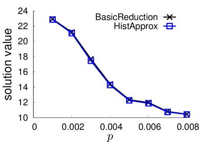
((a)) Solution value (Brightkite)

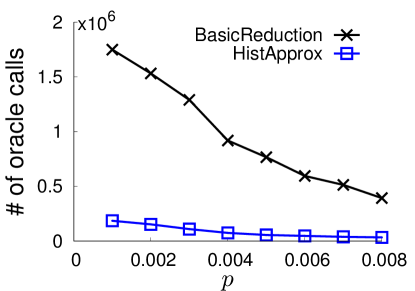
((b)) Efficiency (Brightkite)

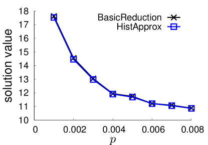
((c)) Solution value (Gowalla)

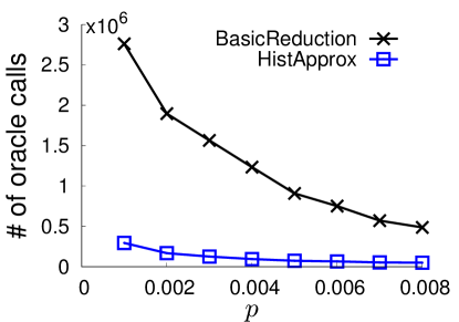
((d)) Efficiency (Gowalla)

Figure 7: Comparing BasicReduction with HistApprox. ($\epsilon=0.1,k=10,L=1000$, each point is averaged over $5000$ time steps)

First, we observe that the solution value of HistApprox is very close to BasicReduction. The solution value ratio of HistApprox to BasicReduction is larger than $0.98$. Second, we observe that the number of oracle calls of BasicReduction decreases as $p$ increases, i.e., more interactions tend to short lifetimes. This observation consists with our analysis that processing edges with long lifetimes is the main bottleneck of BasicReduction. Third, HistApprox needs much less oracle calls than BasicReduction, and the ratio of the number of oracle calls of HistApprox to BasicReduction is less than $0.1$.

This experiment demonstrates that HistApprox outputs solutions with value very close to BasicReduction but is much efficient than BasicReduction.

Evaluating Solution Quality of HistApprox Over Time. We conduct more in-depth analysis of HistApprox in the following experiments. First, we evaluate the solution quality of HistApprox in comparison with other baseline methods.

We run HistApprox with $\epsilon=0.1,0.15$ and $0.2$ for $5000$ time steps on the six datasets, respectively, and maintain $k=10$ nodes at each time step. We compare the solution value of HistApprox with Greedy and Random. The results are depicted in Fig. 8.

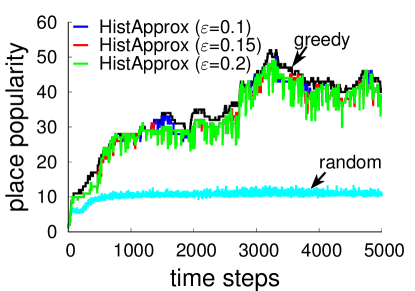
((a)) Brightkite

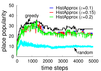
((b)) Gowalla

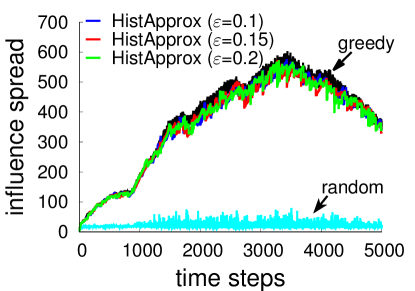
((c)) Twitter-Higgs

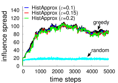
((d)) Twitter-HK

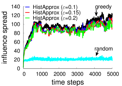
((e)) StackOverflow-c2q

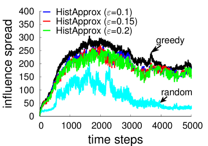
((f)) StackOverflow-c2a

Figure 8: Solution value over time (higher is better). $k=10,L=10K$

We observe that on all of the six datasets, Greedy achieves the highest solution value, and Random achieves the lowest. The solution value of HistApprox is very close to Greedy, and is much better than Random. To clearly judge $\epsilon$’s effect on solution quality, we calculate the ratio of solution value of HistApprox to Greedy, and average the ratios along time, and show the results in Fig. 9. It is clear to see that when $\epsilon$ increases, the solution value decreases in general.

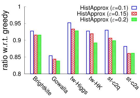
Figure 9: Ratio of solution value averaged along time (higher is better)

These experiments demonstrate that HistApprox achieves comparable solution quality with Greedy, and smaller $\epsilon$ helps improving HistApprox’s solution quality.

Evaluating Computational Efficiency of HistApprox Over Time. Next we compare HistApprox’s computational efficiency with Greedy. When calculating the number of oracle calls of Greedy, we use the lazy evaluation [32] trick, which is a useful heuristic to reduce Greedy’s number of oracle calls.

We run HistApprox with $\epsilon=0.1,0.15$ and $0.2$ on the six datasets, respectively, and calculate the ratio of cumulative number of oracle calls at each time step of HistApprox to Greedy. The results are depicted in Fig. 10.

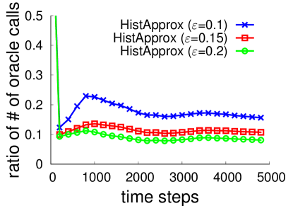
((a)) Brightkite

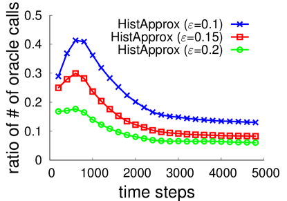
((b)) Gowalla

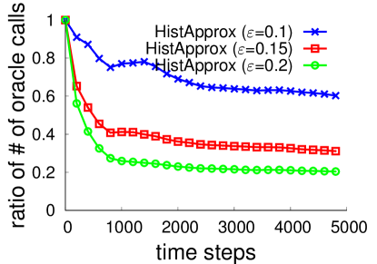
((c)) Twitter-Higgs

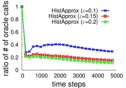
((d)) Twitter-HK

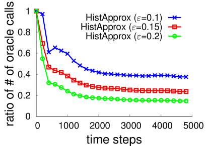
((e)) StackOverflow-c2q

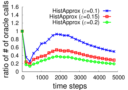
((f)) StackOverflow-c2a

Figure 10: Number of oracle calls ratio (lower is better). $k=10,L=10K$

On all of the six datasets, HistApprox uses much less oracle calls than Greedy. When $\epsilon$ increases, the number of oracle calls of HistApprox decreases further. For example, with $\epsilon=0.2$, HistApprox uses $5$ to $15$ times less oracle calls than Greedy.

This experiment demonstrates that HistApprox is more efficient than Greedy. Combining with the previous results, we conclude that $\epsilon$ can trade off between solution quality and computational efficiency: larger $\epsilon$ makes HistApprox run faster but also decreases solution quality.

Effects of Parameter $k$ and $L$. We evaluate HistApprox’s performance using different budgets $k=10,\ldots,100$ and lifetime upper bounds $L=10K,\ldots,100K$. For each budget $k$ (and $L$), we run HistApprox for $5000$ time steps, and calculate two ratios: (1) the ratio of HistApprox’s solution value to Greedy’s solution value; and (2) the ratio of HistApprox’s number of oracle calls to Greedy’s number of oracle calls. We average these ratios along time, and show the results in Figs. 11 and 12.

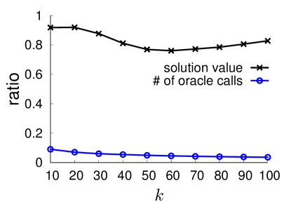
((a)) Brightkite

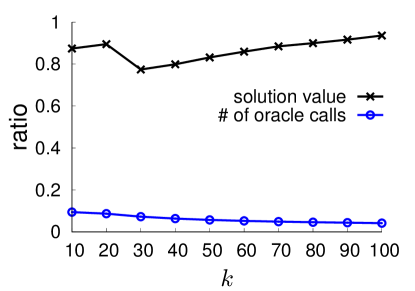
((b)) Gowalla

Figure 11: Performance of HistApprox w.r.t. different $k$. ($\epsilon=0.2,L=10K$. Each point is averaged over $5000$ time steps.)

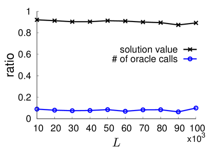
((a)) Brightkite

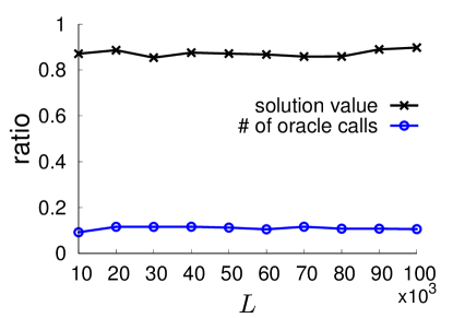
((b)) Gowalla

Figure 12: Performance of HistApprox w.r.t. different $L$. ($\epsilon=0.2,k=10$. Each point is averaged over $5000$ time steps.)

We find that under different parameter settings, HistApprox’s performance consists with our previous observations. In addition, we find that, for larger $k$, the efficiency of HistApprox improves more significantly than Greedy. This is due to the fact that HistApprox’s time complexity increases logarithmically with $k$; while Greedy’s time complexity increases linearly with $k$. We also find that $L$ does not affect HistApprox’s performance very much.

Performance and Throughput Comparisons. Next, we compare the solution quality and throughput with the other baseline methods. Since Greedy achieves the highest solution quality among all the methods, we use Greedy as a reference and show solution value ratio w.r.t. Greedy when evaluating solution quality. For throughput analysis, we will show the maximum stream processing speed (i.e., number of processed edges per second) using different methods.

We set budgets $k=10,\ldots,100$. Lifetimes are sampled from $\textrm{Geo}(0.001)$ with upper bounds $L=10K,\ldots,100K$ respectively. We set $\epsilon=0.3$ in HistApprox. All of the algorithms are ran for $10,000$ time steps. For throughput analysis, we fix the budget to be $k=10$. The results are depicted in Figs. 13 and 14.

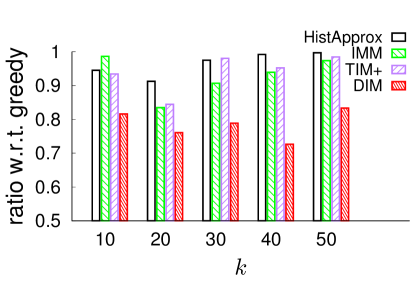
((a)) Twitter-Higgs

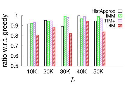
((b)) Twitter-Higgs

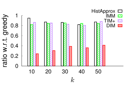
((c)) StackOverflow-c2q

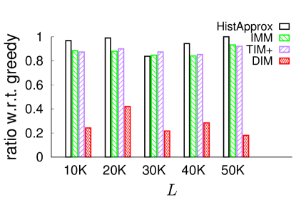
((d)) StackOverflow-c2q

Figure 13: Solution quality comparison (higher is better)

((a)) Twitter-Higgs

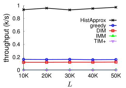
((b)) Twitter-Higgs

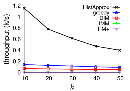
((c)) StackOverflow-c2q

((d)) StackOverflow-c2q

Figure 14: Throughput comparison (higher is better)

From Fig. 13, we observe that HistApprox, IMM and TIM+ always find high quality solutions. In contrast, DIM seems not so stable, and it performs even worse on the StackOverflow-c2q dataset than on the Twitter-Higgs dataset. From Fig. 14, we observe that HistApprox achieves the highest throughput than the other methods, then comes Greedy and DIM, the two methods IMM and TIM+ designed for static graphs have the lowest throughput (and they almost overlap with each other). Greedy using the lazy evaluation trick is faster than DIM, IMM, and TIM+ because the oracle call implementation in Greedy is much faster than oracle call implementations in the other three methods, which relay on Monte-Carlo simulations.

This experiment demonstrates that our proposed HistApprox algorithm can find high quality solutions with high throughput.

VI Related Work

Influence Maximization (IM) over Dynamic Networks. IM and its variants on static networks have been extensively studied (e.g., [1, 2, 3, 4, 5, 6, 7, 8, 9], to name a few). Here we devote to review some literature related to IM on dynamic networks.

Aggarwal et al. [15] and Zhuang et al. [16] propose heuristic approaches to solve IM on dynamic networks. These heuristic approaches, however, have no theoretical guarantee on the quality of selected nodes.

Song et al. [19] use the interchange greedy approach [27] to solve IM over a sequence of networks with the assumption that these networks change smoothly. The interchange greedy approach updates current influential nodes based on influential nodes found in previous network and avoids constructing the solution from an empty set. This approach has an approximation factor $(1/2-\epsilon)$. However, the interchange greedy approach degrades to running from scratch if these networks do not change smoothly. This limits its application on highly dynamic networks.

Both [17] and [18] extend the reverse-reachable (RR) sets [2] to updatable index structures for faster computing the influence of a node or a set of nodes in dynamic networks. In particular, [18] considers finding influential individuals in dynamic networks, which is actually a different problem. It is worth noting that RR-sets are approximation methods designed to speed up the computation of the influence of a set of nodes under the IC or LT model, which is #P-hard; while our approach is a data-driven approach without any assumption of influence spreading model.

There are also some variants of IM on dynamic networks such as topic-specific influencers query [33, 34] and online learning approach for IM [35].

Streaming Submodular Optimization (SSO) Methods. SSO over insertion-only streams is first studied in [36] and the state-of-the-art approach is the threshold based SieveStreaming algorithm [26] which has an approximation factor $(1/2-\epsilon)$.

The sliding-window stream model is first introduced in [22] for maintaining summation aggregates on a data stream (e.g., counting the number of $1$’s in a $0$-$1$ stream). Chen et al. [29] leverage the smooth histogram technique [23] to solve SSO under the sliding-window stream, and achieves a $(1/4-\epsilon)$ approximation factor. Epasto et al. [24] further improve the approximation factor to $(1/3-\epsilon)$.

Note that our problem requires solving SSO over time-decaying streams, which is more general than sliding-window streams. To the best of our knowledge, there is no previous art that can solve SSO on time-decaying streams.

Recently, [25] leveraged the results of [29] to develop a streaming method to solve IM over sliding-window streams. The best approximation factor of their framework is $(1/4-\epsilon)$. In our work, we consider the more general time-decaying stream, and our approach can achieve the $(1/2-\epsilon)$ approximation factor.

Maintaining Time-Decaying Stream Aggregates. Cohen et al. [37] first extend the sliding-window model in [22] to the general time-decaying model for the purpose of approximating summation aggregates in data streams. Cormode et al. [38] consider the similar problem by designing time-decaying sketches. These studies have inspired us to consider the more general time-decaying streams.

VII Conclusion

This work studied the problem of identifying influential nodes from highly dynamic node interaction streams. Our methods are based on a general TDN model which allows discarding outdated data in a smooth manner. We designed three algorithms, i.e., SieveADN, BasicReduction, and HistApprox. SieveADN identifies influential nodes over ADNs. BasicReduction uses SieveADN as a basic building block to identify influential nodes over TDNs. HistApprox significantly improves the efficiency of BasicReduction. We conducted extensive experiments on real interaction datasets and the results demonstrated the efficiency and effectiveness of our methods.

Proof of Theorem 2

The proof goes along the lines of proof in [26] with the major difference that we allow duplicate nodes in the node stream and the time-varying nature of objective $f_{t}$ in our problem.

Let $\mathrm{OPT}_{t}$ denote the value of an optimal solution at time $t$. Let $\Delta_{t}$ denote the maximum value of singletons at time $t$. The threshold set $\Theta$ in SieveADN guarantees that there always exists a threshold $\theta\in\Theta$ falling into interval $[(1-\epsilon)\frac{\mathrm{OPT}_{t}}{2k},(1+\epsilon)\frac{\mathrm{OPT}_{t}}{2k}]$. To see this, because $\Delta_{t}\leq\mathrm{OPT}_{t}\leq k\Delta_{t}$, therefore the smallest threshold in $\Theta$ is at most $(1+\epsilon)\frac{\mathrm{OPT}_{t}}{2k}$. Setting $\theta$ to be the largest threshold in $\Theta$ that does not exceed $(1+\epsilon)\frac{\mathrm{OPT}_{t}}{2k}$ will satisfy the claim.

Let $S_{\theta}^{(t)}$ denote the set of nodes corresponding to threshold $\theta$ maintained in SieveADN at time $t$. We partition set $S_{\theta}^{(t)}$ into two disjoint subsets $S_{\theta}^{(t-1)}$ and $\bar{S}_{\theta}^{(t)}$ where $S_{\theta}^{(t-1)}$ is the maintained nodes at time $t-1$ and $\bar{S}_{\theta}^{(t)}\subseteq\bar{V}_{t}$ is the set of nodes newly selected from $\bar{V}_{t}$ at time $t$. Our goal is to prove that $f_{t}(S_{\theta}^{(t)})\geq(1/2-\epsilon)\mathrm{OPT}_{t}$.

We first inductively show that $f_{t}(S_{\theta}^{(t)})\geq|S_{\theta}^{(t)}|\theta$. Thus if $|S_{\theta}^{(t)}|=k$, then $f_{t}(S_{\theta}^{(t)})\geq k\theta\geq\frac{1-\epsilon}{2}\mathrm{OPT}_{t}$.

At time $t=1$, by definition, $S_{\theta}^{(1)}=\bar{S}_{\theta}^{(1)}$ consists of nodes such that their marginal gains are at least $\theta$. Therefore $f_{1}(S_{\theta}^{(1)})\geq|S_{\theta}^{(1)}|\theta$. Assume it holds that $f_{t-1}(S_{\theta}^{(t-1)})\geq|S_{\theta}^{(t-1)}|\theta$ at time $t-1$, then let us consider $f_{t}(S_{\theta}^{(t)})$ at time $t$:

$$f_{t}(S_{\theta}^{(t)}) =f_{t}(S_{\theta}^{(t-1)}\cup\bar{S}_{\theta}^{(t)})$$

$$=\underset{\text{first part}}{\underbrace{f_{t}(S_{\theta}^{(t-1)}\cup\bar{S}_{\theta}^{(t)})-f_{t}(S_{\theta}^{(t-1)})}}+\underset{\text{second part}}{\underbrace{f_{t}(S_{\theta}^{(t-1)})}}$$

The first part corresponds to the gain of newly selected nodes $\bar{S}_{\theta}^{(t)}$ at time $t$ with respect to the nodes selected previously. Because the newly selected nodes all have marginal gain at least $\theta$, therefore, the first part $\geq|\bar{S}_{\theta}^{(t)}|\theta$.

For the second part, according to the property of ADNs, we have $f_{t}(S_{\theta}^{(t-1)})\geq f_{t-1}(S_{\theta}^{(t-1)})$. Using the induction assumption, it follows that the second part $\geq|S_{\theta}^{(t-1)}|\theta$.

We conclude that $f_{t}(S_{\theta}^{(t)})\geq(|\bar{S}_{\theta}^{(t)}|+|S_{\theta}^{(t-1)}|)\theta=|S_{\theta}^{(t)}|\theta$, and $f_{t}(S_{\theta}^{(t)})\geq\frac{1-\epsilon}{2}\mathrm{OPT}_{t}$ when $|S_{\theta}^{(t)}|=k$.

In the case $|S_{\theta}^{(t)}|<k$, let $S_{t}^{*}$ denote an optimal set of nodes at time $t$. We aim to upper bound the gap between $\mathrm{OPT}_{t}$ and $f_{t}(S_{\theta}^{(t)})$. Using the submodularity of $f_{t}$, we have

$$\mathrm{OPT}_{t}-f_{t}(S_{\theta}^{(t)})$$

$$\leq \sum_{x\in S_{t}^{*}\backslash S_{\theta}^{(t)}}\delta_{S_{\theta}^{(t)}}(x)$$

$$= \sum_{x\in S_{t,1}^{*}\backslash\bar{S}_{\theta}^{(t)}}\delta_{S_{\theta}^{(t)}}(x)+\sum_{y\in S_{t,2}^{*}\backslash S_{\theta}^{(t-1)}}\delta_{S_{\theta}^{(t)}}(y)$$

where $S_{t,1}^{*}\triangleq S_{t}^{*}\cap\bar{V}_{t}$ is the set of optimal nodes in $\bar{V}_{t}$, and $S_{t,2}^{*}\triangleq S_{t}^{*}\backslash S_{t,1}^{*}$ is the set of rest optimal nodes. For the first part, it is obvious that $\delta_{S_{\theta}^{(t)}}(x)<\theta$. For the second part, because $S_{\theta}^{(t-1)}\subseteq S_{\theta}^{(t)}$, then $\delta_{S_{\theta}^{(t)}}(y)\leq\delta_{S_{\theta}^{(t-1)}}(y)$ due to submodularity. By definition,

$$\delta_{S_{\theta}^{(t-1)}}(y) =f_{t}(\{y\}\cup S_{\theta}^{(t-1)})-f_{t}(S_{\theta}^{(t-1)})$$

$$\leq f_{t-1}(\{y\}\cup S_{\theta}^{(t-1)})-f_{t-1}(S_{\theta}^{(t-1)})$$

$$\leq\theta.$$

The first inequality holds due to the fact that the influence spread of $y\notin\bar{V}_{t}$ does not increase at $t$; thus adding edges to the graph at time $t$ cannot increase $y$’s marginal gain. For the second inequality, we continue the reasoning until time $t^{\prime}<t$ when $y\in\bar{V}_{t^{\prime}}$; since $y$ is not selected, then its marginal gain is less than $\theta$. Therefore, it follows that

$$\mathrm{OPT}_{t}-f_{t}(S_{\theta}^{(t)})\leq k\theta\leq k(1+\epsilon)\frac{\mathrm{OPT}_{t}}{2k}=\frac{1+\epsilon}{2}\mathrm{OPT}_{t},$$

which implies $f_{t}(S_{\theta}^{(t)})\geq\frac{1-\epsilon}{2}\mathrm{OPT}_{t}$.

Because SieveADN outputs a set of nodes whose value is at least $f_{t}(S_{\theta}^{(t)})$, we thus conclude that SieveADN achieves an $(1/2-\epsilon)$ approximation factor. ∎

Proof of Theorem 3

Notice that set $\Theta$ contains $\log_{1+\epsilon}2k=O(\epsilon^{-1}\log k)$ thresholds. For each node, we need to calculate the marginal gains $|\Theta|$ times and each uses time $O(\gamma)$. Thus, for $|\bar{V}_{t}|=b$ nodes, the time complexity is $O(b\gamma\epsilon^{-1}\log k)$. SieveADN needs to maintain sets $\{S_{\theta}\colon\theta\in\Theta\}$ in memory. Each set has cardinality at most $k$, and there are $|\Theta|=O(\epsilon^{-1}\log k)$ sets at any time. Thus the space complexity is $O(k\epsilon^{-1}\log k)$. ∎

Proof of Theorem 6

If $x_{i+1}^{\prime}$ became the successor of $x_{i}^{\prime}$ due to the removal of indices between them at some most recent time $t^{\prime}\leq t$, then procedure ReduceRedundancy in Alg. 3 guarantees that $g_{t^{\prime}}(x_{i+1}^{\prime})\geq(1-\epsilon)g_{t^{\prime}}(x_{i}^{\prime})$ after the removal at time $t^{\prime}$. From time $t^{\prime}$ to $t$, it is also impossible to have edge with lifetime between the two indices arriving. Otherwise we will meet a contradiction: either these edges form redundant SieveADN instances again thus $t^{\prime}$ is not the most recent time as claimed, or these edges form non-redundant SieveADN instances thus $x_{i}$ and $x_{i+1}$ cannot be consecutive at time $t$. We thus get C2.

Otherwise $x_{i+1}^{\prime}$ became the successor of $x_{i}^{\prime}$ when one of them is inserted in the histogram at some time $t^{\prime}\leq t$. Without lose of generality, let us assume $x_{i+1}^{\prime}$ is inserted after $x_{i}^{\prime}$ at time $t^{\prime}$. If edges with lifetimes between the two indices arrive from time $t^{\prime}$ to $t$, these edges must form redundant SieveADN instances. We still get C2. Or, there is no edge with lifetime between the two indices at all, i.e., $G_{t}$ contains no edge with lifetime between $x_{i}$ and $x_{i+1}$. We get C1. ∎

Proof of Theorem 7

If $x_{1}=1$ at time $t$, then $\mathcal{A}_{1}^{(t)}$ exists. By Theorem 4, we have $g_{t}(x_{1})=g_{t}(1)\geq(1/2-\epsilon)\mathrm{OPT}_{t}$.

Otherwise we have $x_{1}>1$ at time $t$. If $G_{t}$ contains edges with lifetime less than $x_{1}$, then $\mathcal{A}_{x_{1}}^{(t)}$ does not process all of the edges in $G_{t}$, thus incurs a loss of solution quality. Our goal is to bound this loss.

Let $x_{0}$ denote the most recent expired predecessor of $x_{1}$ at time $t$, and let $t^{\prime}<t$ denote the last time $x_{0}$’s ancestor $x_{0}^{\prime}$ was still alive, i.e., $x_{0}^{\prime}=1$ at time $t^{\prime}$ (refer to Fig. 15). For ease of presentation, we commonly refer to $x_{0}$ and $x_{0}$’s ancestors as the left index, and refer to $x_{1}$ and $x_{1}$’s ancestors as the right index. Obviously, in time interval $(t^{\prime},t]$, no edge with lifetime less than the right index arrives; otherwise, these edges would create new indices before the right index; then $x_{1}$ will not be the first index at time $t$, or $x_{0}$ is not the most recent expired predecessor of $x_{1}$ at time $t$.

Figure 15: Indices relations at time $t^{\prime\prime}\leq t^{\prime}<t$. $x_{0}$ (resp. $x_{1}$) and its ancestors are commonly referred to as the left (right) index.

Notice that $x_{0}^{\prime}$ and $x_{1}^{\prime}$ are two consecutive indices at time $t^{\prime}$. By Theorem 6, we have two cases.

• If C1 holds. In this case, $G_{t^{\prime}}$ contains no edge with lifetime between $x_{0}^{\prime}$ and $x_{1}^{\prime}$. Because there is also no edge with lifetime less than the right index from time $t^{\prime}$ to $t$, then $G_{t}$ has no edge with lifetime less than $x_{1}$ at time $t$. Therefore, $\mathcal{A}_{x_{1}}^{(t)}$ processed all of the edges in $G_{t}$. By Theorem 4, we still have $g_{t}(x_{1})=g_{t}(1)\geq(1/2-\epsilon)\mathrm{OPT}_{t}$.

• If C2 holds. In this case, there exists time $t^{\prime\prime}\leq t^{\prime}$ s.t. $g_{t^{\prime\prime}}(x_{1}^{\prime\prime})\geq(1-\epsilon)g_{t^{\prime\prime}}(x_{0}^{\prime\prime})$ holds (refer to Fig. 15), and from time $t^{\prime\prime}$ to $t^{\prime}$, no edge with lifetime between the two indices arrived (however $G_{t}$ may have edges with lifetime less than $x_{1}$ at time $t$ and these edges arrived before time $t^{\prime\prime}$). Notice that edges with lifetime no larger than the left index all expired after time $t^{\prime}$ and they do not affect the solution at time $t$; therefore, we can safely ignore these edges in our analysis and only care edges with lifetime no less than the right index arrived in interval $[t^{\prime\prime},t]$. Notice that these edges are only inserted on the right side of the right index.

In other words, at time $t^{\prime\prime}$, the output values of the two instances satisfy $g_{t^{\prime\prime}}(x_{1}^{\prime\prime})\geq(1-\epsilon)g_{t^{\prime\prime}}(x_{0}^{\prime\prime})$; from time $t^{\prime\prime}$ to $t$, the two instances are fed with same edges. Such a scenario has been studied in the sliding-window case [24]. By the submodularity of $f_{t}$ and monotonicity of the SieveADN algorithm, the following lemma guarantees that $g_{t}(x_{1})$ is close to $\mathrm{OPT}_{t}$.

Lemma 1 ([24]).

Consider a cardinality constrained monotone submodular function maximization problem. Let $\mathcal{A}(S)$ denote the output value of applying the SieveStreaming algorithm on stream $S$. Let $S\|S^{\prime}$ denote the concatenation of two streams $S$ and $S^{\prime}$. If $\mathcal{A}(S_{2})\geq(1-\epsilon)\mathcal{A}(S_{1})$ for $S_{2}\subseteq S_{1}$ (i.e., each element in stream $S_{2}$ is also an element in stream $S_{1}$), then $\mathcal{A}(S_{2}\|S)\geq(1/3-\epsilon)\mathrm{OPT}$ for all $S$, where $\mathrm{OPT}$ is the value of an optimal solution in stream $S_{1}\|S$.

In our scenario, at time $t^{\prime\prime}$ the two instances satisfy $g_{t^{\prime\prime}}(x_{1}^{\prime\prime})\geq(1-\epsilon)g_{t^{\prime\prime}}(x_{0}^{\prime\prime})$ and $\mathcal{A}_{x_{1}^{\prime\prime}}$’s input is a subset of $\mathcal{A}_{x_{0}^{\prime\prime}}$’s input. After time $t^{\prime\prime}$, the two instances are fed with same edges. Because SieveADN preserves the property of SieveStreaming, hence our case can be mapped to the scenario in Lemma 1. We thus obtain $g_{t}(x_{1})\geq(1/3-\epsilon)\mathrm{OPT}_{t}$.

Combining the above results, we conclude that HistApprox guarantees a $(1/3-\epsilon)$ approximation factor. ∎

Proof of Theorem 8

At any time $t$, because $g_{t}(x_{i+2})<(1-\epsilon)g_{t}(x_{i})$, and $g_{t}(l)\in[\Delta,k\Delta]$, then the size of index set $\mathbf{x}_{t}$ is upper bounded by $O(\log_{(1-\epsilon)^{-1}}k)=O(\epsilon^{-1}\log k)$. For each batch of edges, in the worst case, we need to update $|\mathbf{x}_{t}|$ SieveADN instances, and each SieveADN instance has update time $O(b\gamma\epsilon^{-1}\log k)$ according to Theorem 3. In addition, procedure ReduceRedundancy has time complexity $O(\epsilon^{-2}\log^{2}k)$ and it is called at most $b$ times. Thus the total time complexity is $O(b(\gamma+1)\epsilon^{-2}\log^{2}k)$.

For memory usage, because HistApprox maintains $|\mathbf{x}_{t}|$ SieveADN instances, and each instance uses memory $O(k\epsilon^{-1}\log k))$ according to Theorem 3. Thus the total memory used by HistApprox is $O(k\epsilon^{-2}\log^{2}k))$. ∎

References

- [1] D. Kempe, J. Kleinberg, and E. Tardos, “Maximizing the spread of influence through a social network,” in KDD, 2003.
- [2] C. Borgs, M. Brautbar, J. Chayes, and B. Lucier, “Maximizing social influence in nearly optimal time,” in SODA, 2014.
- [3] W. Chen, C. Wang, and Y. Wang, “Scalable influence maximization for prevalent viral marketing in large-scale social networks,” in KDD, 2010.
- [4] Y. Tang, X. Xiao, and Y. Shi, “Influence maximization: Near-optimal time complexity meets practical efficiency,” in SIGMOD, 2014.
- [5] B. Lucier, J. Oren, and Y. Singer, “Influence at scale: Distributed computation of complex contagion in networks,” in KDD, 2015.
- [6] Y. Tang, Y. Shi, and X. Xiao, “Influence maximization in near-linear time: A martingale approach,” in KDD, 2015.
- [7] W. Chen, T. Lin, Z. Tan, M. Zhao, and X. Zhou, “Robust influence maximization,” in KDD, 2016.
- [8] I. Litou, V. Kalogeraki, and D. Gunopulos, “Influence maximization in a many cascades world,” in ICDCS, 2017.
- [9] Y. Lin, W. Chen, and J. C. Lui, “Boosting information spread: An algorithmic approach,” in ICDE, 2017.
- [10] K. Saito, R. Nakano, and M. Kimura, “Prediction of information diffusion probabilities for independent cascade model,” in KES, 2008.
- [11] A. Goyal, F. Bonchi, and L. V. S. Lakshmanan, “Learning influence probabilities in social networks,” in WSDM, 2010.
- [12] K. Kutzkov, A. Bifet, F. Bonchi, and A. Gionis, “STRIP: Stream learning of influence probabilities,” in KDD, 2013.
- [13] S. Myers and J. Leskovec, “The bursty dynamics of the Twitter information network,” in WWW, 2014.
- [14] S. Myers, C. Zhu, and J. Leskovec, “Information diffusion and external influence in networks,” in KDD, 2012.
- [15] C. Aggarwal, S. Lin, and P. S. Yu, “On influential node discovery in dynamic social networks,” in SDM, 2012.
- [16] H. Zhuang, Y. Sun, J. Tang, J. Zhang, and X. Sun, “Influence maximization in dynamic social networks,” in ICDM, 2013.
- [17] N. Ohsaka, T. Akiba, Y. Yoshida, and K. Kawarabayashi, “Dynamic influence analysis in evolving networks,” in VLDB, 2016.
- [18] Y. Yang, Z. Wang, J. Pei, and E. Chen, “Tracking influential individuals in dynamic networks,” TKDE, vol. 29, no. 11, pp. 2615–2628, 2017.
- [19] G. Song, Y. Li, X. Chen, X. He, and J. Tang, “Influential node tracking on dynamic social network: An interchange greedy approach,” TKDE, vol. 29, no. 2, pp. 359–372, 2017.
- [20] R. Xiang, J. Neville, and M. Rogati, “Modeling relationship strength in online social networks,” in WWW, 2010.
- [21] N. Alon, Y. Matias, and M. Szegedy, “The space complexity of approximating the frequency moments,” Journal of Computer and System Sciences, vol. 58, no. 1, pp. 137–147, 1999.
- [22] M. Datar, A. Gionis, P. Indyk, and R. Motwani, “Maintaining stream statistics over sliding windows,” SIAM Journal on Computing, vol. 31, no. 6, pp. 1794–1813, 2002.
- [23] V. Braverman and R. Ostrovsky, “Smooth histograms for sliding windows,” in FOCS, 2007.
- [24] A. Epasto, S. Lattanzi, S. Vassilvitskii, and M. Zadimoghaddam, “Submodular optimization over sliding windows,” in WWW, 2017.
- [25] Y. Wang, Q. Fan, Y. Li, and K.-L. Tan, “Real-time influence maximization on dynamic social streams,” in VLDB, 2017.
- [26] A. Badanidiyuru, B. Mirzasoleiman, A. Karbasi, and A. Krause, “Streaming submodular maximization: Massive data summarization on the fly,” in KDD, 2014.
- [27] G. Nemhauser, L. Wolsey, and M. Fisher, “An analysis of approximations for maximizing submodular set functions - i,” Mathematical Programming, vol. 14, pp. 265–294, 1978.
- [28] “TechReport,” https://arxiv.org/pdf/1810.07917.pdf.
- [29] J. Chen, H. L. Nguyen, and Q. Zhang, “Submodular maximization over sliding windows,” in arXiv:1611.00129, 2016.
- [30] “Stanford network dataset,” http://snap.stanford.edu/data.
- [31] J. Zhao, J. C. Lui, D. Towsley, P. Wang, and X. Guan, “Tracking triadic cardinality distributions for burst detection in social activity streams,” in COSN, 2015.
- [32] M. Minoux, “Accelerated greedy algorithms for maximizing submodular set functions,” Optimization Techniques, vol. 7, pp. 234–243, 1978.
- [33] K. Subbian, C. Aggarwal, and J. Srivastava, “Content-centric flow mining for influence analysis in social streams,” in CIKM, 2013.
- [34] K. Subbian, C. C. Aggarwal, and J. Srivastava, “Querying and tracking influencers in social streams,” in WSDM, 2016.
- [35] S. Lei, S. Maniu, L. Mo, R. Cheng, and P. Senellart, “Online influence maximization,” in KDD, 2015.
- [36] R. Kumar, B. Moseley, S. Vassilvitskii, and A. Vattani, “Fast greedy algorithms in MapReduce and streaming,” in SPAA, 2013.
- [37] E. Cohen and M. J. Strauss, “Maintaining time-decaying stream aggregates,” Journal of Algorithms, vol. 59, pp. 19–36, 2006.
- [38] G. Cormode, S. Tirthapura, and B. Xu, “Time-decaying sketches for robust aggregation of sensor data,” SIAM Journal on Computing, vol. 39, no. 4, pp. 1309–1339, 2009.