Time-optimal Control of Independent Spin-$\frac{1}{2}$ Systems under Simultaneous Control

Abstract

We derive the explicit solution of the problem of time-optimal control by a common magnetic fields for two independent spin-$\frac{1}{2}$ particles. Our approach is based on the Pontryagin Maximum Principle and a novel symmetry reduction technique. We experimentally implement the optimal control using zero-field nuclear magnetic resonance. This reveals an average gate error of $1\%$ and a $70\%$ to $80$ $\%$ decrease in the experiment duration as compared to existing methods. This is the first analytical solution and experimental demonstration of time-optimal control in such a system and it provides a route to achieve time optimal control in more general quantum systems.

I Introduction

Time-optimal control (TOC) problems in quantum systems are ubiquitous and important in multiple applications Shapiro2003 ; Schulte2005 ; Ernst1990 ; glasereuro . Because the inevitable noise from the environment degrades quantum states and operations over time, inducing quantum dynamics in minimal time utilizing TOC becomes a preferable choice. Different mathematical approaches exist to obtain accurate TOC protocols Carlini2006 ; Rezakhani2009 ; Wang2015 ; Geng2016 , with the Pontryagin Maximum Principle (PMP) Sachkov unifying some of them. However, independently of the method used, analytic solutions are rare in optimal control and often a numerical prescription is given for the optimal control law with known problems of convergence to the actual solution Rao ; Chen2015 . Previous works mainly consider time optimization with controls which address spin individually Khaneja2002 ; Yuan2005 . However this is difficult in many experiments, and control of all spins simultaneously affected is a common scenario.

In this paper, we use the Pontryagin Maximum Principle (PMP) (see, e.g., Sachkov ) and a novel symmetry reduction technique Albertini2018 , to obtain the optimal control laws for a system of two uncoupled spin-$\frac{1}{2}$ particles, under simultaneous control. Our symmetry reduction technique allows us to reduce the number of unknown parameters and to obtain analytic solutions. We implemented the TOC law using zero-field NMR Blanchard2016 , obtaining experimental fidelity as high as $99\%$ and a gain of about $70\%\sim 80\%$ in the experiment time over previously known schemes Bian2017 ; Jiang2017 .

In particular, our model is as follows: Two spin-$\frac{1}{2}$ particles with different gyromagnetic ratios $\gamma_{1}$ and $\gamma_{2}$ are simultaneously subject to a global (spatially uniform) control field $\vec{u}(t):=u_{x,y,z}$. The Hamiltonian is $H(\vec{u})=\sum_{j=x,y,z}(\gamma_{1}\sigma_{j}\otimes{\bf 1}_{2}+\gamma_{2}{\bf 1}_{2}\otimes\sigma_{j})u_{j}$, where $\vec{\sigma}=\sigma_{x,y,z}$ are the Pauli matrices,

$$\sigma_{x}=\begin{pmatrix}0&1\cr 1&0\end{pmatrix},\qquad\sigma_{y}=\begin{pmatrix}0&-i\cr i&0\end{pmatrix},\qquad\sigma_{z}=\begin{pmatrix}1&0\cr 0&-1\end{pmatrix},\qquad$$

and ${\bf 1}_{n}$ denotes the $n\times n$ identity. The problem is to steer the identity ${\bf 1}_{4}\in\textrm{SU}(4)$ to any desired matrix $U_{f,1}\otimes U_{f,2}\in\textrm{SU}(2)\otimes\textrm{SU}(2)$ under a constraint of the form $|\vec{u}|\leq D$, $D\not=0$. We assume $\gamma_{1}\not=\gamma_{2}$ (heteronuclear spins) f1 which implies controllability Mikobook in $\textrm{SU}(2)\otimes\textrm{SU}(2)$, that is, every operator in $\textrm{SU}(2)\otimes\textrm{SU}(2)$ can be reached with an appropriate (arbitrarily bounded) control. Let ${\cal B}$ be the subspace in $\textrm{su}(2)\oplus\textrm{su}(2)$ defined as ${\cal B}:=\texttt{span}\{i\sigma_{x}\otimes{\bf 1}_{2}+\gamma{\bf 1}_{2}\otimes i\sigma_{x},-i\sigma_{y}\otimes{\bf 1}_{2}-\gamma{\bf 1}_{2}\otimes i\sigma_{y},i\sigma_{z}\otimes{\bf 1}_{2}+\gamma{\bf 1}_{2}\otimes i\sigma_{z}\}$ with $\gamma:=\gamma_{2}/\gamma_{1}$. The problem of optimal control can be stated as finding a function $X:=X(t)=-iH(\vec{u})$ with values in ${\cal B}$, where $H$ is the above Hamiltonian, so that the solution of the Schrödinger operator equation,

$$\dot{U}=X(t)U\qquad U(0)={\bf 1}_{4},$$ (1)

reaches $U_{f,1}\otimes U_{f,2}$ in minimum time. Using the Hamiltonian of the system, we have $X=-i\sum_{j=x,y,z}(\gamma_{1}\sigma_{j}\otimes{\bf 1}_{2}+\gamma_{2}{\bf 1}_{2}\otimes\sigma_{j})u_{j}$ and the knowledge of $X=X(t)$ is equivalent to the knowledge of the control $\vec{u}$. Moreover the bound on the control in the optimal control problem implies a bound on the norm of $X$. In particular $|\vec{u}|\leq D$ if and only if

$$\|X(t)\|\leq\tilde{L}:=|\gamma_{1}|\sqrt{1+\gamma^{2}}D$$ (2)

for all $t$. [The inner product in $\textrm{su}(n)$ (in particular for $n=4$) is $\langle A,B\rangle:=\frac{1}{n}\textrm{Tr}(AB^{\dagger})$ so that $\|A\|:=\frac{1}{\sqrt{n}}\sqrt{\text{Tr}(AA^{\dagger})}$.]

This paper is organized as follows: In section II we describe the method to obtain TOC, i.e., PMP and symmetry reduction technique. A step-by-step protocol, and a flow chart (Figure 2) illustrating the algorithm to obtain TOC are also summarized in this section. In section III, in preparation to the experiments we carried out, we consider the special case where we want to perform a rotation on the first spin while leaving the second spin unchanged. We prove that, in this case, the core step of the proposed algorithm amounts to an integer optimization problem with constraints (Theorem 2). We apply this method to our experiment in section IV, together with an evaluation of the quality of the control. The conclusion and discussion of this work is given in Section V. Some useful computations and extra considerations are collected in the appendix.

II Time-optimal control law

We combine the PMP on Lie groups Sachkov with the use of symmetry reduction Albertini2018 . This results in an algorithm to obtain the optimal control laws.

II.1 The PMP and the form of optimal control

The following theorem which uses the Pontryagin Maximum Principle for systems on Lie groups Sachkov gives a description of the functional form of the optimal control and trajectory.

Theorem 1.

Write $X=-i\sum_{j=x,y,z}(\sigma_{j}\otimes{\bf 1}_{2}+\gamma{\bf 1}_{2}\otimes\sigma_{j})u_{j}:=X_{1}\otimes{\bf 1}_{2}+\gamma{\bf 1}_{2}\otimes X_{1}$ (so that $X_{1}:=\sum_{j=x,y,z}-i\sigma_{j}u_{j}$) the optimal control, and $U:=U_{1}\otimes U_{2}$ the optimal trajectory. Then there exist matrices $P$ and $A$ in $\textrm{su}(2)$ such that

$$X_{1}=e^{At}P{e^{-At}},\>U_{1}=e^{At}e^{(P-A)t},\>U_{2}=e^{At}e^{(\gamma P-A)t}.$$ (3)

Proof. Consider the controlled dynamics (1). Conditions given by PMP for right invariant systems on Lie groups Sachkov say that if $X=X(t)$ and $U=U(t)$ is an optimal pair of control and trajectory, respectively, in time $t_{\textrm{min}}$, then the following facts hold true: There exists a nonzero pair $(F,\lambda_{0})$ with $F$ in the associated Lie algebra, in this case $\textrm{su}(2)\oplus\textrm{su}(2)$, and $\lambda_{0}$ a scalar such that, defined the (PMP) Hamiltonian $\tilde{H}(F,\hat{U},V):=\langle F,\hat{U}^{\dagger}V\hat{U}\rangle$, with $\hat{U}$ in the given Lie group, in this case $\textrm{SU}(2)\otimes\textrm{SU}(2)$, and $V$ in the control set, in this case $V\in{\cal B}$, so that, for almost every $t\in[0,t_{\textrm{min}}]$,

$$\tilde{H}(F,U(t),X(t))=\max_{\|V\|\leq\tilde{L}}\tilde{H}(F,U(t),V)=\lambda_{0}.$$ (4)

By applying the Goh condition (see, e.g., Appendix C in OptRes and references therein) it also follows that $\lambda_{0}\not=0$ and therefore $F\not=0$ as well footnote1 .

Define $F:=F_{1}\otimes{\mathbf{1}_{2}}+{\mathbf{1}_{2}}\otimes F_{2}\in\textrm{su}(2)\oplus\textrm{su}(2)$, and recall $U:=U_{1}\otimes U_{2}$ and $X:=X_{1}\otimes{\bf 1}_{2}+\gamma{\bf 1}_{2}\otimes X_{1}$. We have

$$\tilde{H}(F,U,X):=\langle F,U^{\dagger}XU\rangle$$ (5)

$$=\langle U_{1}F_{1}U_{1}^{\dagger}\otimes{\bf 1}_{2}+{\bf 1}_{2}\otimes U_{2}F_{2}U_{2}^{\dagger},X_{1}\otimes{\bf 1}_{2}+\gamma{\bf 1}_{2}\otimes X_{1}\rangle$$

$$=\langle\tilde{B}+\gamma\tilde{C},X_{1}\rangle,$$

where we used

$$\tilde{B}:=U_{1}F_{1}U_{1}^{\dagger},\qquad\tilde{C}:=U_{2}F_{2}U_{2}^{\dagger}.$$ (6)

Furthermore, $\tilde{B}+\gamma\tilde{C}$ is never zero since this would imply $\lambda_{0}=0$ in the PMP. From the Cauchy-Schwartz inequality for the inner product $\langle A,B\rangle=\frac{1}{2}\textrm{Tr}(AB^{\dagger})$ in $\textrm{su}(2)$ and the bound on $X$ which gives a constant bound on $X_{1}$, from (4) there exists a constant $k$ such that $X_{1}:=\frac{k(\tilde{B}+\gamma\tilde{C})}{\|\tilde{B}+\gamma\tilde{C}\|}$ (recall that the norm of $X$ and therefore the norm of $X_{1}$ is constant footnote2 ). Replacing this into the last one of (5), we have

$$\tilde{H}(F,U,X)=2k\|\tilde{B}+\gamma\tilde{C}\|=\lambda_{0}\not=0,$$ (7)

which implies that $\|\tilde{B}+\gamma\tilde{C}\|$ is constant. Therefore denoting by $B$ and $C$ the matrix functions obtained from $\tilde{B}$ and $\tilde{C}$ in (6) by possibly re-scaling $F_{1}$ and $F_{2}$, we have, for the form of the optimal control,

$$X=X_{1}\otimes{\mathbf{1}}+\gamma{\mathbf{1}}\otimes X_{1},\quad\texttt{with}\quad X_{1}=B+\gamma C,$$ (8)

and

$$B:=B(t)=U_{1}(t)\hat{F}_{1}U_{1}^{\dagger}(t),$$ (9)

$$C:=C(t)=U_{2}(t)\hat{F}_{2}U_{2}^{\dagger}(t),$$ (10)

for matrices $\hat{F}_{1}$ and $\hat{F}_{2}$ (rescaled $F_{1}$ and $F_{2}$) in $\textrm{su}(2)$. The above derived optimal control candidates in (8) are in ‘feedback form’, that is, they depend on the current value of the state of the system, $U_{1}\otimes U_{2}$. We now transform them into the explicit form given in the statement of the theorem. From (1), using (8), we have that the optimal trajectory is $U_{1}\otimes U_{2}$ with

$$\dot{U}_{1}=X_{1}U_{1},\qquad U_{1}(0)={\mathbf{1}}_{2},$$ (11)

$$\dot{U}_{2}=\gamma X_{1}U_{2},\qquad U_{2}(0)={\mathbf{1}}_{2}.$$ (12)

Using (11) and differentiating $B$ in (9), we obtain with (11)

$$\dot{B}=[X_{1},B],\qquad B(0)=\hat{F}_{1},$$ (13)

and from $X_{1}$ in (8), we have

$$\dot{B}=\gamma[C,B],\qquad B(0)=\hat{F}_{1},$$ (14)

Analogously for $C$ we obtain

$$\dot{C}=\gamma[B,C],\qquad C(0)=\hat{F}_{2}.$$ (15)

By combining (14) and (15), we have that

$$\dot{B}+\dot{C}\equiv 0.$$ (16)

Therefore $B+C=\tilde{A}$, for a constant $\tilde{A}\in\textrm{su}(2)$. Therefore, from (8) we have

$$X_{1}(t)=(1-\gamma)B(t)+\gamma\tilde{A}.$$ (17)

Replacing this in (13) and solving we obtain that $B(t)=e^{\gamma\tilde{A}t}\hat{F}_{1}e^{-\gamma\tilde{A}t}$, which replaced in (17) gives

$$X_{1}(t)=e^{\gamma\tilde{A}t}\left((1-\gamma)\hat{F}_{1}+\gamma\tilde{A}\right)e^{-\gamma\tilde{A}t}.$$ (18)

By choosing $A:=\gamma\tilde{A}$ and $P=(1-\gamma)\hat{M}_{1}+\gamma\tilde{A}$, and solving (11), (12), one obtains:

$$X_{1}=e^{At}P{e^{-At}},\,U_{1}=e^{At}e^{(P-A)t},\,$$

$$U_{2}=e^{At}e^{(\gamma P-A)t},$$

which are formula (3). This completes the proof of the theorem.

Theorem 1 reduces the search of the optimal control on a space of functions to the search for the matrices $A$ and $P$ in $\textrm{su}(2)$. Using Theorem 1, the TOC problem is then to find two matrices $A$ and $P$ in $\textrm{su}(2)$ and the minimum of $t$, such that $U(t)=e^{At}e^{(P-A)t}\otimes e^{At}e^{(\gamma P-A)t}=U_{f,1}\otimes U_{f,2}$, for desired final conditions $U_{f,1}$ and $U_{f,2}$ for systems $1$ and $2$, respectively. From the theorem we need $U_{1}(t)=e^{At}e^{(P-A)t}=\pm U_{f,1}$ and $U_{2}(t)=e^{At}e^{(\gamma P-A)t}=\pm U_{f,2}$, with minimum $t$. The only constraint on $A$ and $P$ in $\textrm{su}(2)$ is (cf. (2))

$$\|P\| =\|X_{1}\|=\frac{1}{\sqrt{1+\gamma^{2}}}\|X\|$$ (19)

$$:=\tilde{L}/\sqrt{1+\gamma^{2}}=|\gamma_{1}|D:=L,$$

which is a consequence of the bound on the control. This results in six parameters to be chosen. However, a reduction of the number of parameters can be achieved using the symmetry of the problem Albertini2018 as explained next.

Remark II.1.

The matrices $A$ and $P$ in the theorem, which are used in the expression of the optimal control, depend on the parameter $\gamma$. This is true also for the minimum time $t$. At the limit $\gamma\rightarrow 1$ the system (1) loses controllability on $\textrm{SU}(2)\otimes\textrm{SU}(2)$ in that the operations at the limit are the same on the two spins. This implies that, except for very special final conditions, the minimum time goes to $\infty$ as $\gamma$ tends to $1$. This can be seen from the expressions of the trajectories $U_{1}$ and $U_{2}$ in (3). We can write $U_{1}U_{2}^{\dagger}$ as

$$U_{1}U_{2}^{\dagger}=e^{At}e^{(P-A)t}e^{(-\gamma P+A)t}e^{-At}=$$

$$e^{At}e^{(P-A)t}e^{(-P+A)t+(1-\gamma)Pt}e^{-At}.$$

This has to be a fixed matrix for a desired final condition. If, by contradiction, we assume that $t=t(\gamma)$ is bounded as $\gamma$ goes to $1$ the term $(1-\gamma)Pt$ will tend to zero (since $P$ is also bounded because of the bound on the control). Therefore the matrix on the right hand side will tend to the identity which is true only for final operations equal to each other on the two systems.

II.2 Symmetry reduction

Let $G$ be the Lie subgroup of $\textrm{SU}(2)\otimes\textrm{SU}(2)$ of matrices of the form $Y\otimes Y$ with $Y\in\textrm{SU}(2)$. The Lie group $G$ acts on $\textrm{SU}(2)\otimes\textrm{SU}(2)$ by conjugation, i.e., for $U\in\textrm{SU}(2)\otimes\textrm{SU}(2)$, $Y\otimes Y\in G$, as $U\rightarrow(Y\otimes Y)U(Y^{\dagger}\otimes Y^{\dagger})$. With this action, $G$ is a group of symmetries for the time optimal control problem in the sense of Albertini2018 . This implies that if $X:=X(t)$ is an optimal control and $U:=U(t)$ is the corresponding optimal trajectory for a final condition $U_{f}$, then, for any fixed $Y\otimes Y\in G$, $(Y\otimes Y)X(Y^{\dagger}\otimes Y^{\dagger})$ is an optimal control and $(Y\otimes Y)U(Y^{\dagger}\otimes Y^{\dagger})$ the corresponding optimal trajectory for the final condition $(Y\otimes Y)U_{f}(Y^{\dagger}\otimes Y^{\dagger})$ with the same minimum time. A direct way to see this is to consider equation (1) with $X$ the optimal control to reach $U_{f}$, defining $\hat{Y}:=Y\otimes Y$. By multiplying (1) on the left by $\hat{Y}$ and on the right by $\hat{Y}^{\dagger}$ we obtain a differential equation for $\hat{Y}U\hat{Y}^{\dagger}$. $\hat{Y}X\hat{Y}^{\dagger}$ is again an admissible control since it still belongs to ${\cal B}$ and its norm is the same as the one of $X$. Therefore we have an admissible control which drives to $\hat{Y}U_{f}\hat{Y}^{\dagger}$ in the same time as the minimum time to drive to $U_{f}$. Moreover this is the minimum time also for $\hat{Y}U_{f}\hat{Y}^{\dagger}$. If there was a shorter time, this would imply (repeating the argument) a shorter time for $U_{f}$ which contradicts optimality. Summarizing, if we find the optimal control and trajectory for a final condition $U_{f}$, we have found the optimal control and trajectory for any final condition of the type $(Y\otimes Y)U_{f}(Y^{\dagger}\otimes Y^{\dagger})$. $U_{f}$ and $(Y\otimes Y)U_{f}(Y^{\dagger}\otimes Y^{\dagger})$ are said to be in the same orbit. It is sufficient to find the optimal control and trajectory for one representative in the desired orbit in order to find optimal controls for all elements in the orbit. We can use this fact to reduce the number of parameters we look for in the optimal control.

Given $A$ and $P$ in $\textrm{su}(2)$, choose $Y_{1}\in\textrm{SU}(2)$ diagonalizing $A$ ($Y_{1}A{Y_{1}}^{\dagger}=i\omega\sigma_{z}$). Also let $Y_{2}\in\textrm{SU}(2)$ diagonal and such that $Y_{2}Y_{1}PY_{1}^{\dagger}Y_{2}^{\dagger}=i(a\sigma_{z}-b\sigma_{y})$ with $\sqrt{a^{2}+b^{2}}=L$ (cf. (19)). Then $U_{1}\otimes U_{2}$ from Theorem 1 is in the same orbit as $\tilde{U}:=\tilde{U}_{1}\otimes\tilde{U}_{2}:=YU_{1}Y^{\dagger}\otimes YU_{2}Y^{\dagger}$ with $Y:=Y_{1}Y_{2}$. Here:

$$YU_{1}Y^{\dagger}=Ye^{At}e^{(P-A)t}Y^{\dagger}=e^{i\omega\sigma_{z}t}e^{(ia\sigma_{z}-ib\sigma_{y}-i\omega\sigma_{z})t},$$ (20)

$$YU_{2}Y^{\dagger}=Ye^{At}e^{(\gamma P-A)t}Y^{\dagger}=e^{i\omega\sigma_{z}t}e^{(i\gamma a\sigma_{z}-i\gamma b\sigma_{y}-i\omega\sigma_{z})t}.$$

Consequently the (TOC) problem of searching for six parameters is reduced to the problem of searching for three independent parameters, i.e., $\omega$, $t_{min}$ and $(a,b)$ with $(\sqrt{a^{2}+b^{2}}=L)$. The parameter $t_{\textrm{min}}$ is the minimum time $t$ such that $YU_{1}Y^{\dagger}\otimes YU_{2}Y^{\dagger}$, in (20) is in the same orbit as the desired $U_{f,1}\otimes U_{f,2}$.

The control $(Y\otimes Y)X(Y^{\dagger}\otimes Y^{\dagger})=YX_{1}Y^{\dagger}\otimes{\bf 1}_{2}+\gamma{\bf 1}_{2}\otimes YX_{1}Y^{\dagger}$, with $YX_{1}Y^{\dagger}=e^{i\omega\sigma_{z}t}(ia\sigma_{z}-ib\sigma_{y})e^{-i\omega\sigma_{z}t}$ drives the state optimally from the identity ${\bf 1}_{4}$ to an element in the same orbit as $U_{f,1}\otimes U_{f,2}$. The problem is therefore split in two. First one chooses the parameters $\omega$, $a$ ($b$) and $t=t_{\textrm{min}}$ to reach the orbit of $U_{f,1}\otimes U_{f,2}$ and then one ‘adjusts’ via a similarity transformation of the form $Y\otimes Y$ to obtain exactly the desired final condition $U_{f,1}\otimes U_{f,2}$.

In order to follow this procedure we need an explicit description of the space of orbits, $SU(2)\otimes SU(2)/G$, the orbit space footnote3 . To simplify the problem, we slightly relax the equivalence relation on $\textrm{SU}(2)\otimes\textrm{SU}(2)$ to a relation, $\sim_{\times}$, on $\textrm{SU}(2)\times\textrm{SU}(2)$, so that $(W_{1},Z_{1})\sim_{\times}(W_{2},Z_{2})$ if and only if there exists a $Y$ in $\textrm{SU}(2)$ such that $(W_{2},Z_{2})=(YW_{1}Y^{\dagger},YZ_{1}Y^{\dagger})$. We have that $W_{1}\otimes Z_{1}$ and $W_{2}\otimes Z_{2}$ are in the same orbit if and only if $(W_{1},Z_{1})\sim_{\times}(W_{2},Z_{2})$ or $(W_{1},Z_{1})\sim_{\times}(-W_{2},-Z_{2})$, i.e., two points in the orbit space $\textrm{SU}(2)\times\textrm{SU}(2)/\sim_{\times}$ correspond to the same point in the orbit space $SU(2)\otimes SU(2)/G$. The characterization of $\textrm{SU}(2)\otimes\textrm{SU}(2)/\sim_{\times}$ is given in the following proposition. The proof is reported in the Appendix section VI.1 voronov . Here ${\bf D}$ denotes the closed unit disc in the complex plane, that is, the set of complex numbers $x\in\mbox{${\rm\>C\!\!\!I\;\;}$}$ such that $|x|\leq 1$.

Proposition II.2.

There exists a one to one and onto map $\Psi$

$$\Psi: (\textrm{SU}(2)\times\textrm{SU}(2))/\sim_{\times}\longrightarrow$$ (21)

$$\left((0,\pi)\times{\bf D}\right)\bigcup\left(\{0\}\times[0,\pi]\right)\bigcup\left(\{\pi\}\times[0,\pi]\right),$$

defined as follows:

1. If $U$ has an eigenvalue $e^{i\phi}$, with $\phi\in(0,\pi)$ and therefore $U:=S\Lambda S^{\dagger}$ with $S\in\textrm{SU}(2)$ and $\Lambda:=\begin{pmatrix}e^{i\phi}&0\cr 0&e^{-i\phi}\end{pmatrix}$ then

   $$\Psi\left([(U,Z)]\right)=(\phi,(S^{\dagger}ZS)_{1,1})\in(0,\pi)\times{\bf D},$$ (22)

   where $(S^{\dagger}ZS)_{1,1}$ denotes the $(1,1)$ entry of the matrix $S^{\dagger}ZS$ which is an element of ${\bf D}$, and $[(U,Z)]$ denotes the orbit with representative $(U,Z)$ ($[(U,Z)]\in(\textrm{SU}(2)\times\textrm{SU}(2))/\sim_{\times}$).

2. If $U$ is the identity matrix ${\bf 1}_{2}$ and $e^{i\psi}$ with $\psi\in[0,\pi]$ is an eigenvalue of $Z$ then

   $$\Psi\left([(U,Z)]\right)=(0,\psi)\in\{0\}\times[0,\pi].$$ (23)

3. If $U$ is the negative of the identity matrix, i.e., $-{\bf 1}_{2}$, and $e^{i\psi}$ with $\psi\in[0,\pi]$ is an eigenvalue of $Z$ then

   $$\Psi\left([(U,Z)]\right)=(\pi,\psi)\in\{\pi\}\times[0,\pi].$$ (24)

Topologically therefore the orbit space $\textrm{SU}(2)\times\textrm{SU}(2)/\sim_{\times}$ looks like a deformed solid cylinder as in Figure 1, where the discs at the left and right ends are degenerate to a segment ($[0,\pi]$), and every other cross section is (homeomorphic to) a disc.

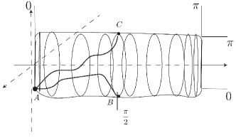
Figure 1: Representation of the Orbit Space $\textrm{SU}(2)\times\textrm{SU}(2)/\sim_{\times}$. The point $A$ corresponds to the equivalence class $[({\bf 1}_{2},{\bf 1}_{2})]$; The point $B$ corresponds to the equivalence class $[(\textrm{Phase},{\bf 1_{2}})]$ with Phase gate defined in (83) and $C$ corresponds to the equivalence class $[(\textrm{Phase},-{\bf 1_{2}})]$. Trajectories are depicted in the orbit space joining $A$ and $B$, $A$ and $C$.

Since $\Psi$ in the proposition is a bijection $(U_{1},Z_{1})\sim_{\times}(U_{2},Z_{2})$ if and only if $\Psi([(U_{1},Z_{1})])=\Psi([(U_{2},Z_{2})])$. Therefore a test for $\sim_{\times}$ equivalence is given in the following corollary.

Corollary II.3.

$(U_{1},Z_{1})\sim_{\times}(U_{2},Z_{2})$ if and only if one of the following occurs: 1) $U_{1}=U_{2}=\pm{\bf 1}_{2}$ and the spectrum of $Z_{1}$ is equal to the spectrum of $Z_{2}$; 2) $U_{1}:=S_{1}\Lambda S_{1}^{\dagger}$ and $U_{2}:=S_{2}\Lambda S_{2}^{\dagger}$ for the same diagonal $\Lambda$ theorm2note , (with $S_{1}$ and $S_{2}$ in $\textrm{SU}(2)$) and $(S_{1}^{\dagger}Z_{1}S_{1})_{1,1}=(S_{2}^{\dagger}Z_{2}S_{2})_{1,1}$ where $R_{1,1}$ denotes the $(1,1)$ entry of the matrix $R$.

Proof. The case 1 of the corollary corresponds to the cases 2 and 3 of the proposition. The case 2 of the corollary corresponds to the case 1 of the proposition.

Analysis on quotient spaces in the context of quantum optimal control was also done in Khan1 . The quotient space in Khan1 is a symmetric space Helgason while the one described in the above proposition and corollary is a stratified space Snyaticki .

II.3 Procedure to obtain the time optimal control

Combining the explicit form of the optimal control obtained in subsection II.1 with the symmetry reduction described in subsection II.2, the main points of the protocol to find the optimal control field can be summarized as follows.

1. The PMP gives the form of optimal control $X=\sum_{j=x,y,z}-i(\sigma_{j}\otimes{\bf 1}+\gamma{\bf 1}\otimes\sigma_{j})u_{j}=X_{1}\otimes{\bf 1}+\gamma{\bf 1}\otimes X_{1}$, and trajectory, $U(t)=U_{1}(t)\otimes U_{2}(t)$. These are given by $X_{1}=e^{At}Pe^{-At}$, $U_{1}=e^{At}e^{(P-A)t}$, $U_{2}=e^{At}e^{(\gamma P-A)t}$, where $A$ and $P$ are constants in $\textrm{su}(2)$, parametrized therefore by $6$ real parameters.

2. Symmetry reduction further reduces the number of unknown parameters to 3: If the control $X$ and trajectory $U$ are an optimal pair with optimal time $t_{\textrm{min}}$, then $\hat{Y}X\hat{Y}^{\dagger}$ and $\hat{Y}U\hat{Y}^{\dagger}$ is also an optimal pair with $t_{\textrm{min}}$ (20). There are, $\omega,t_{\textrm{min}},a$ $(b)$, with $\sqrt{a^{2}+b^{2}}=L$, 3 unknown parameters to be determined now ($\hat{Y}$ is also unknown, but it can be determined if the above three parameters are known).

3. Find real values $\omega$, $t=t_{\textrm{min}}$, $a$ ($b$) (see point 1 above and (20)), such that

   $$\qquad(e^{i\omega\sigma_{z}t}e^{(ia\sigma_{z}-ib\sigma_{y}-i\omega\sigma_{z})t},e^{i\omega\sigma_{z}t}e^{(i\gamma a\sigma_{z}-i\gamma b\sigma_{y}-i\omega\sigma_{z})t})$$

   is in the same class as $(U_{f,1},U_{f,2})$ (Use Corollary II.3), and $t$ is minimum.

4. Repeat step 3 with the substitution: $(U_{f,1},U_{f,2})\rightarrow(-U_{f,1},-U_{f,2})$. Choose the minimum time between these two cases, and the corresponding $\omega,t:=t_{\textrm{min}},a$ $(b)$.

5. Find $Y\in\textrm{SU}(2)$ such that

   $$\pm U_{f,1}=Y^{\dagger}e^{i\omega\sigma_{z}t}e^{(ia\sigma_{z}-ib\sigma_{y}-i\omega\sigma_{z})t}Y,$$

   $$\pm U_{f,2}=Y^{\dagger}e^{i\omega\sigma_{z}t}e^{(i\gamma a\sigma_{z}-i\gamma b\sigma_{y}-i\omega\sigma_{z})t}Y,$$

   with $t=t_{\textrm{min}}$. The $\pm$ sign is chosen according to step 4.

6. The optimal control is $X:=X_{1}\otimes{\bf 1}_{2}+\gamma{\bf 1}_{2}\otimes X_{1}$ with $X_{1}:=Y^{\dagger}e^{i\omega\sigma_{z}t}(ia\sigma_{z}-ib\sigma_{y})e^{-i\omega\sigma_{z}t}Y$.

A simplification in the above procedure is obtained assuming for $L$ in (19) $L:=\sqrt{a^{2}+b^{2}}=1$, that is, normalizing the bound $D$ on the control. We can always recover the optimal control for the original problem. In fact, if $\vec{u}_{N}(t)$ is the optimal control with a bound $\frac{1}{|\gamma_{1}|}$ ($L=1$) in time $t_{N}$, $\vec{u}(t)=L\vec{u}_{N}(Lt)=|\gamma_{1}|Du_{N}(|\gamma_{1}|Dt)$ will be an optimal control for a general bound $D$, in minimum time $\frac{t_{N}}{L}$. We shall therefore set $L=1$ in the following discussion. FIG. 2 gives a flow chart of the algorithm to find the optimal control. This algorithm takes the desired final condition $U_{f,1}\otimes U_{f,2}$ as the input and obtains the time optimal control.

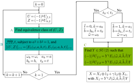
Figure 2: Flow chart of the procedure to find the optimal control $X=X_{1}\otimes{\bf 1}_{2}+\gamma{\bf 1}\otimes X_{1}$. For brevity, we use the notation $E_{\gamma}(\omega,a,b,t):=e^{i\omega\sigma_{z}t}e^{i(\gamma a\sigma_{z}-\gamma b\sigma_{y}-\omega\sigma_{z})t}$ and $J(\omega,a,b,t):=e^{i\omega\sigma_{z}t}(ia\sigma_{z}-ib\sigma_{y})e^{-i\omega\sigma_{z}t}$.

The routine $A$ of the flow chart is carried out using corollary II.3 and proposition II.2. It amounts to a standard eigenvalue-eigenvector problem for which in general there are many available numerical algorithms and in our case can be solved by hand since we are dealing with $2\times 2$ matrices. Task $C$ is the solution of a system of linear equations in which we can use any available parametrization of matrices in $SU(2)$. It corresponds to step $5$ of the previously described protocol. The solution of the minimization problem in $B$ which corresponds to task $3$ of the protocol is arguably the most difficult step of the algorithm and the core of our solution method. We shall often refer in the following to this step as ‘Task 3’. One method to tackle this step is to use the concept of reachable set as discussed in Albertini2018 . Consider the geometric description of the orbit space $\textrm{SU}(2)\times\textrm{SU}(2)/\sim_{\times}$ given in Figure 1. This can be depicted (from Corollary II.3) as a solid cylinder where the two extreme discs are collapsed to a segment. The orbit of a pair $(\pm U_{f,1},\pm U_{f,2})$ is a point in this space. If we fix $t$ and vary $\omega$ and $a$ ($b$), we obtain a surface in this $3-$D space which is the boundary of the set of orbits reachable at time $t$. The first $t$ such that this surface includes the desired point is the minimum time. The values of $\omega$ and $a$ ($b$) where the intersection occurs are the optimal values for the parameters. Alternatively one can directly tackle the optimization problem to minimize $t$ under the constraint that the pair

$$(e^{i\omega\sigma_{z}t}e^{i(a\sigma_{z}-b\sigma_{y}-\omega\sigma_{z})t},e^{i\omega\sigma_{z}t}e^{i(\gamma a\sigma_{z}-\gamma b\sigma_{y}-\omega\sigma_{z})t})$$ (25)

is in the same equivalence class (with respect to the equivalence relation $\sim_{\times}$) as $(U_{f,1},U_{f,2})$, using the explicit computations of matrix exponentials which are reported in the Appendix (section VI.2). This problem is in some cases simplified and can be solved analytically, as in the application to our experiments which we discuss next.

III Application to selective single-spin rotations

We applied the above procedure to obtain the TOC law for selective rotations on the first spin, i.e., $U_{f}=U_{f,1}\otimes U_{f,2}=e^{-i\mathbf{n}\cdot\vec{\sigma}\frac{\theta}{2}}\otimes\mathbf{1}_{2}$, where $\mathbf{n}$ is a unit vector and the rotation angle $\theta$ is chosen in $(0,2\pi)$. The possible final conditions in $\textrm{SU}(2)\times\textrm{SU}(2)$ are $(e^{-i\mathbf{n}\cdot\vec{\sigma}\frac{\theta}{2}},{\bf 1}_{2})$ and $(-e^{-i\mathbf{n}\cdot\vec{\sigma}\frac{\theta}{2}},-{\bf 1}_{2})$. Since $U_{f,2}=\pm\mathbf{1}_{2}$ is invariant under similarity transformations, the parameters in step 3 of the above procedure ( routine $B$ in FIG. 2) have to be chosen so that in (20) $e^{i\omega\sigma_{z}t}e^{(i\gamma a\sigma_{z}-i\gamma b\sigma_{y}-i\omega\sigma_{z})t}=\pm\mathbf{1}_{2}$. This implies that $i\gamma a\sigma_{z}-i\gamma b\sigma_{y}-i\omega\sigma_{z}t$, and therefore $b\sigma_{y}$, commutes with $e^{-i\omega\sigma_{z}t}$ which is diagonal. Therefore $e^{-i\omega\sigma_{z}t}=\pm{\bf 1}_{2}$ or $b=0$. If $b=0$ ($a=\pm 1$), the final conditions give $\gamma t=k\pi$ and $\cos(t)=(-1)^{k}\cos(\frac{\theta}{2})$. So, in this case, we choose as candidate minimum time $t=|\frac{k}{\gamma}|\pi$ where $|k|$ is the smallest integer (if any) such that $\cos(|\frac{k}{\gamma}|\pi)=(-1)^{k}\cos(\frac{\theta}{2})$. If $b\not=0$ ($|a|<1$), the problem to minimize $t$ subject to the final condition (i.e., Task 3) can be transformed into an integer optimization problem as summarized in the following theorem:

Theorem 2.

Assume that the optimal parameters are such that $b\not=0$ in Task 3. Define the function

$$M_{\gamma}(s,m,l,k):=m^{2}(1-\gamma)+(s\frac{\theta}{2\pi}+l)^{2}\gamma-k^{2},$$ (26)

where $s=\pm 1$ and $m,l,k$ are integers with $m,k>0$, and $l,k$ share the same parity if $\theta\not=\pi$. When $s=1$, $l\geq 0$; when $s=-1$, $l>0$. Then the minimum time $t$, $t_{min}$, is the minimum value of $\pi\sqrt{\frac{M_{\gamma}(s,m,l,k)}{\gamma(1-\gamma)}}$, with the constraint

$$[m-s\frac{\theta}{2\pi}-l]^{2}<\frac{M_{\gamma}(s,m,l,k)}{\gamma(1-\gamma)}<[m+s\frac{\theta}{2\pi}+l]^{2}.$$ (27)

With, $t=t_{min}$ and the optimal $(s,m,l,k)$ the corresponding parameters $(\omega,a,b)$ are given by $\omega=\frac{m\pi}{t}$, $a=\frac{\omega}{2\gamma}+\frac{\gamma}{2\omega}-\frac{k^{2}\pi}{2tm\gamma}$, and $b=\pm\sqrt{1-a^{2}}$

Proof. Using the calculation of exponential of matrices in section VI.2, and the conditions on the final state for the first spin, we obtain

$$(e^{i\omega t}+e^{-i\omega t})\cos(\eta_{1}t)=\pm 2\cos{(\frac{\theta}{2})}.$$ (28)

This is in particular obtained taking the trace of the matrix in (81) and imposing that it is equal to ($\pm$) the trace of the desired final condition. By imposing that the matrix in (82) is equal to $\pm$ the identity, we get

$$e^{i\omega t}(\cos(\eta_{\gamma}t)+i\frac{\gamma a-\omega}{\eta_{\gamma}}\sin(\eta_{\gamma}t))=\pm 1.$$ (29)

In these formulas, we used the definitions $\eta_{1}:=\sqrt{\omega^{2}+1-2a\omega}$, $\eta_{\gamma}:=\sqrt{\omega^{2}+\gamma^{2}-2a\omega\gamma}$. From (29), since $|a|<1$ and recall the definition of $\eta_{\gamma}$, we obtain the two conditions

$$\omega t=m\pi,$$ (30)

$$\eta_{\gamma}t:=\sqrt{\omega^{2}+\gamma^{2}-2\gamma a\omega}\,t=k\pi,$$ (31)

for integers $m$ and $k>0$. Using (30) in (28), and the fact that whether we use $+$ or $-$ depends on $(-1)^{m}(-1)^{k}$ from (31), (30) and (29) we obtain $(-1)^{m}2\cos(\eta_{1}t)=2(-1)^{m}(-1)^{k}\cos(\frac{\theta}{2})$, that is,

$$\cos(\eta_{1}t)=(-1)^{k}\cos(\frac{\theta}{2}).$$ (32)

Therefore, in particular we have

$$\eta_{1}t:=\sqrt{\omega^{2}+1-2a\omega}\,t=s\frac{\theta}{2}+l\pi,\\$$ (33)

with $l$ and $k$ having the same parity if $\theta\not=\pi$. Therefore the condition on the final state is verified if and only if conditions (30), (31) and (33) are verified with $l$ and $k$ having the same parity if $\theta\not=\pi$.

If $\omega=0$ then $m=0$ from (30), and (31), (33) give $t=\frac{|k|}{|\gamma|}\pi$ and $\cos(t)=(-1)^{k}\cos(\frac{\theta}{2})$. So the situation is the same as the one discussed for $b=0$ and therefore we can avoid considering this case as for now we assume that the optimal occurs (only) for $b\not=0$. Therefore we assume $\omega\not=0$. We can in fact assume $\omega>0$, and therefore $m>0$ also, since for every pair $(\omega,a)$ satisfying (30), (31), (33) for a certain $t$, the pair $(-\omega,-a)$ also satisfies (30), (31), (33) with the same $t$.

Now using (30) in (31) and (33), we obtain

$$m\sqrt{\omega^{2}+\gamma^{2}-2a\gamma\omega}=\omega k,$$ (34)

and

$$m\sqrt{\omega^{2}+1-2a\omega}=s\frac{q}{2}\omega+l\omega.$$ (35)

with $\theta=q\pi,q=(0,2)$. We have that if $s=1$, $l\geq 0$, while if $s=-1$, $l$ must be $>0$. Eliminating $a\omega$ by combining equations (35) and (34), we obtain that

$$\omega^{2}=\frac{m^{2}\gamma(1-\gamma)}{M_{\gamma}(s,m,l,k)},$$ (36)

with $M_{\gamma}(s,m,l,k)\gamma(1-\gamma)>0.$ ($M_{\gamma}(s,m,l,k)$ is defined in 26)

For a certain quadruple $(s,m,l,k)$, the time is then (from (30))

$$t=\frac{m\pi}{\omega}=\pi\sqrt{\frac{M_{\gamma}}{\gamma(1-\gamma)}}.$$ (37)

Using $\omega=\frac{m\pi}{t}$ in (33), we obtain

$$\pi^{2}\left[m^{2}-(s\frac{q}{2}+l)^{2}\right]+t^{2}=2am\pi t,$$ (38)

The condition $|a|<1$ is equivalent to the fact that the absolute value of the right hand side of (38) is strictly less than $2m\pi t$. By setting

$$\left\{\pi^{2}\left[m^{2}-(s\frac{q}{2}+l)^{2}\right]+t^{2}\right\}^{2}<4m^{2}\pi^{2}t^{2},$$ (39)

we obtain the condition for $t^{2}$,

$$[m\pi-(s\frac{q}{2}+l)\pi]^{2}<t^{2}<[m\pi+(s\frac{q}{2}+l)\pi]^{2}.$$ (40)

Replacing (37) in this, we have

$$[m-s\frac{q}{2}-l]^{2}<\frac{M_{\gamma}(s,m,l,k)}{\gamma(1-\gamma)}<[m+s\frac{q}{2}+l]^{2},$$ (41)

which is the same as (27) if we recall that $\theta=q\pi$. We remark that this is in fact the only condition since the left inequality in (41) implies $M_{\gamma}(s,m,l,k)\gamma(1-\gamma)>0$. Using the values of $\omega$ and $t$ in (31) one obtains the expression for $a$ (and therefore $b$) in the statement of the theorem. Theorem 2 transforms Task 3 of the procedure into an integer optimization problem.

Remark III.1.

Given the particular final condition, the sign of $b$ in the statement of the theorem is arbitrary. It does not affect the eigenvalues of the transformation on the first spin given that the transformation on the second spin is the identity.

Remark III.2.

From the proof of the theorem it follows that we have simultaneously considered the case $U\otimes{\bf 1}$ and $(-U)\otimes(-{\bf 1})$ therefore we do not need, in this case, to perform the test ‘$t_{0}<t_{1}$’ in the algorithm of FIG.2, and we can directly move on to the task in $C$ of the flow chart, in this case.

There is no general algorithm to solve the optimization problem of Theorem 2 which treats $\gamma$ as a free parameter. However when $\gamma$ is given a numerical value, such a problem can usually be solved. One possible technique is to use a $min-min$ strategy as follows: First for given $l$ and $m$ one finds the minimum or maximum (according to the sign of $\gamma(1-\gamma)$) value of $k$ (with the same parity of $l$) so that condition (41) is verified. This is because the minimization of $t$ corresponds to the minimization of $\frac{M_{\gamma}}{\gamma(1-\gamma)}$ (from (37)) and $M_{\gamma}$ is given in (26). Such an optimal $k$ will be a function of $l$ and $m$. Then one finds $l$ and $m$ to minimize $t$ in (37). Such a procedure might have to be repeated for $s=1$ and $s=-1$ and the optimal times compared. As an illustration of this technique we consider the case $\gamma=\frac{1}{2}$ in the appendix (section VI.3). Alternatively, one can apply enumeration or numerical search in the space of $(m,l,k)$ to get an optimal candidate, then independently prove its time optimality. This is the technique we have used in our experimental implementation as it is described in the next section.

IV Experiments in zero-field NMR

At zero field, all spins have identical (zero) Larmor frequencies and they cannot be addressed by separate control fields. They can be manipulated by applying pulsed magnetic fields $\vec{B}$ along three directions acting on all the spins. The main advantage of zero-field NMR is that it does not need superconducting magnets. This makes the experiment set-up more flexible compared to high-field NMR. When the control fields satisfy the condition $\gamma_{1,2}|\vec{B}|\gg|2\pi J|$ (the general case in liquid-state NMR experiments), where $J$ is the spin-spin coupling constant, the spin systems at zero field behave as independent spins in simultaneous control.

We experimentally demonstrated the above TOC pulses for an ¹H-¹³C system, i.e., ¹³C-formic acid (¹H-¹³COOH), at zero field. This system is schematically depicted in FIG. 3.

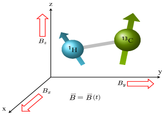
Figure 3: Schematic representation of the control via a spatially uniform magnetic field $\vec{B}$ of the ${}^{1}\textrm{H}$-${}^{13}\textrm{C}$ system.

The ¹H-¹³C spin-spin constant is $J\approx 221.9~{}\textrm{Hz}$ and the lifetime of singlet-triplet coherence Emondts2014 is $T_{2}\approx 2.0~{}\textrm{s}$. For the ¹H-¹³C system, $\frac{\gamma_{\textrm{C}}}{\gamma_{\textrm{H}}}\approx 0.2514=\gamma$. We describe next how to solve the optimization problem of Theorem 2 and obtain the TOC for this value of $\gamma$.

IV.1 Determination of TOC

We now determine the time optimal control for the case of $\gamma:=0.2514$ which corresponds to our experiment, and therefore this value of $\gamma$ will be assumed in this subsection. We start with an ansatz for $M_{\gamma}$ (and therefore $t_{min}$) solving the optimization problem of Theorem 2. This is given by $s=l=k=m=1$, i.e., $M_{\gamma}(1,1,1,1)$. It is achieved by enumeration in a small range [in the space of $(s,m,l,k)$]. However its time optimality cannot be proved by simple enumeration since the triple in $(m,l,k)$ is not in a bounded range.

IV.1.1 Proof of optimality of $M_{\gamma}(1,1,1,1)$

We only consider the case with $q\in(0,1]$ (recall the definition $\theta=q\pi$) since the case $q\in(1,2)$ can be treated similarly. We show that there is no admissible quadruple $(s,m,l,k)$ which gives a value of $M_{\gamma}(s,m,l,k)$ strictly less than $M_{\gamma}(1,1,1,1)$. There are two subcases to consider $s=1$ and $s=-1$.

Case $s=1$

Define $\delta:=m-l$ in $M_{\gamma}(s,m,l,k)=M_{\gamma}(1,m,l,k)$. We first observe the following fact:

Lemma IV.1.

If $M_{\gamma}(1,m,l,k)<M_{\gamma}(1,1,1,1)$ then $\delta=0$ or $\delta=1$

Proof. Using $M_{\gamma}(1,m,l,k)<M_{\gamma}(1,1,1,1)$ the lower bound $(m-l-\frac{q}{2})^{2}$ in (41) gives

$$(m-l-\frac{q}{2})^{2}<\frac{M_{\gamma}(1,1,1,1)}{\gamma(1-\gamma)}.$$ (42)

Direct computation of $M_{\gamma}(1,1,1,1)$ gives $M_{\gamma}(1,1,1,1)=\left(\frac{q^{2}}{4}+q\right)\gamma$, using this in (42) and setting $\delta:=m-l$, we get

$$-\frac{\sqrt{\frac{q^{2}}{4}+q}}{\sqrt{1-\gamma}}+\frac{q}{2}<\delta<\frac{\sqrt{\frac{q^{2}}{4}+q}}{\sqrt{1-\gamma}}+\frac{q}{2}.$$ (43)

This leads to a restriction on the possible values of $\delta$ (recall $\gamma=0.2514$) as claimed:

$$\delta=\left\{\begin{array}[]{ll}0&0<q\leq\frac{2(-8743+50\sqrt{32458})}{1257}(\approx 0.42)\\ 0\ \text{or}\ 1&\frac{2(-8743+50\sqrt{32458})}{1257}<q\leq 1\end{array}\right.$$ (46)

The following two propositions consider the two cases $\delta=0$ and $\delta=1$ and show that, in these cases, there is no quadruple $(1,m,l,k)$ such that $M_{\gamma}(1,m,l,k)<M_{\gamma}(1,1,1,1)$, so completing the proof for the case $s=1$.

Proposition IV.2.

Assume $\delta:=m-l=0$. Then $M_{\gamma}(1,m,l,k)=M_{\gamma}(1,m,m,k)\geq M_{\gamma}(1,1,1,1)$, for any admissible values of $m$, $l$ and $k$.

Proof. If $\delta=0$, $m=l$ gives $M_{\gamma}=m^{2}-k^{2}+\frac{q^{2}}{4}\gamma+mq\gamma$. Since $M_{\gamma}>0$ we must have $m\geq k$. In fact, if $m<k$, we would have

$$M_{\gamma}=m^{2}+qm\gamma-k^{2}+\frac{q^{2}}{4}\gamma\leq(k-1)^{2}+q(k-1)\gamma-k^{2}+\frac{q^{2}}{4}\gamma\leq$$

$$-3+q\gamma+\frac{q^{2}}{4}\gamma<0,$$

which is a contradiction. Set $\epsilon:=m-k$ $(0\leq\epsilon<m)$, $\epsilon$ integer. Assuming by contradiction that $M_{\gamma}(1,m,l,k)<M_{\gamma}(1,1,1,1)$ with the additional requirement that $m=l$ leads to the inequality

$$m^{2}-k^{2}+mq\gamma<q\gamma.$$

Replacing $k$ with $m-\epsilon$, after some algebraic manipulations, we obtain

$$\epsilon<m<\frac{q\gamma+\epsilon^{2}}{q\gamma+2\epsilon},$$ (47)

which leads to:

$$\epsilon^{2}+q\gamma\epsilon-q\gamma<0.$$ (48)

From (48), we have that the only possibility is $\epsilon=0$. Therefore $m=k$. Together with $\delta=0$, this indicates $m=l=k$. However

$$M_{\gamma}(1,m,m,m)=\frac{q^{2}}{4}\gamma+qm\gamma\geq\frac{q^{2}}{4}\gamma+q\gamma=M_{\gamma}(1,1,1,1),$$

with equality valid if and only if $m=1$. Therefore no smaller $M_{\gamma}$ can be found in this case.

Proposition IV.3.

Assume $\delta:=m-l=1$. Then $M_{\gamma}(1,m,l,k)=M_{\gamma}(1,m,m-1,k)\geq M_{\gamma}(1,1,1,1)$, for any admissible values of $m$, $l$ and $k$.

Proof. If $\delta=1$ (corresponding to the second case in (46)), by using $M_{\gamma}$ in (26) with $l=m-1$, $M_{\gamma}>0$ becomes:

$$m^{2}-k^{2}+m(q\gamma-2\gamma)+\gamma+\frac{q^{2}}{4}\gamma-q\gamma>0$$ (49)

Since

$$m(q\gamma-2\gamma)+\gamma+\frac{q^{2}}{4}\gamma-q\gamma <q\gamma-2\gamma+\gamma+\frac{q^{2}}{4}\gamma-q\gamma$$ (50)

$$=-\gamma+\frac{q^{2}}{4}\gamma<0,$$

we must have $m>k$ to make (49) hold. Set $k=m-\epsilon$ ($0<\epsilon<m$, $\epsilon$ integer). Then assuming by contradiction $M_{\gamma}(1,m,l,k)<M_{\gamma}(1,1,1,1)$ (cf. (26)), with $l=m-\delta=m-1$, we obtain

$$m(2\epsilon+q\gamma-2\gamma)<2q\gamma-\gamma+\epsilon^{2}.$$ (51)

Thus:

$$\epsilon<m<\frac{2q\gamma-\gamma+\epsilon^{2}}{2\epsilon+q\gamma-2\gamma}.$$ (52)

From the condition $\frac{2(-8743+50\sqrt{32458})}{1257}<q\leq 1$, we have:

$$-1 <\frac{2\gamma-q\gamma-\sqrt{(q\gamma-2\gamma)^{2}-4(\gamma-2q\gamma)}}{2}<\epsilon<$$ (53)

$$\frac{2\gamma-q\gamma+\sqrt{(q\gamma-2\gamma)^{2}-4(\gamma-2q\gamma)}}{2}<1$$

So no $\epsilon$ satisfies this requirement.

We have thus shown for the case $s=1$ that $M_{\gamma}(1,1,1,1)$ is the minimum.

Case $s=-1$

The following lemma analogous to Lemma IV.1 says that there are two cases again to consider. We set again $\delta:=m-l$.

Lemma IV.4.

If $M_{\gamma}(-1,m,l,k)<M_{\gamma}(1,1,1,1)$ then $\delta=0$ or $\delta=-1$

Proof. From the constraint (41) on $M_{\gamma}$ written for $s=-1$, we know that if $M_{\gamma}(s,m,l,k)$ is strictly less than $M_{\gamma}(1,1,1,1)$, with the lower bound (41) now equal to $(m-l+\frac{q}{2})^{2}$, we must have:

$$(m-l+\frac{q}{2})^{2}<\frac{M_{\gamma}(s,m,l,k)}{\gamma(1-\gamma)}<\frac{M_{\gamma}(1,1,1,1)}{\gamma(1-\gamma)}.$$ (54)

Inequality (54) gives:

$$-\frac{\sqrt{\frac{q^{2}}{4}+q}}{\sqrt{1-\gamma}}-\frac{q}{2}<\delta<\frac{\sqrt{\frac{q^{2}}{4}+q}}{\sqrt{1-\gamma}}-\frac{q}{2},$$ (55)

which leads to the restrictions on $\delta$ (recall $\gamma=0.2514$):

$$\delta=\left\{\begin{array}[]{ll}0&0<q\leq\frac{2(-8743+50\sqrt{32458})}{1257}\\ -1\ \text{or}\ 0&\frac{2(-8743+50\sqrt{32458})}{1257}<q\leq 1\end{array}\right.$$ (58)

The following two propositions consider the cases $\delta=0$ and $\delta=-1$ separately and show that it is not possible in these cases that $M_{\gamma}(-1,m,l,k)<M_{\gamma}(1,1,1,1)$. This is analogous to what has been done in Propositions IV.2 and IV.3 and completes all the subcases, thus showing the optimality of $M_{\gamma}(1,1,1,1)$.

Proposition IV.5.

Assume $\delta:=m-l=0$. Then $M_{\gamma}(-1,m,l,k)=M_{\gamma}(-1,m,m,k)\geq M_{\gamma}(1,1,1,1)$, for any admissible values of $m$, $l$ and $k$.

Proof. If $\delta=0$, we have $M_{\gamma}=M_{\gamma}(-1,m,m,k)=m^{2}-k^{2}+\frac{q^{2}}{4}\gamma-qm\gamma$. From $M_{\gamma}>0$ we must have $m>k$. Set $\epsilon:=m-k$ ($0<\epsilon<m)$, $\epsilon$ integer. The assumption, by contradiction, $M_{\gamma}(-1,m,m,k)<M_{\gamma}(1,1,1,1)$ gives

$$\epsilon<m<\frac{q\gamma+\epsilon^{2}}{2\epsilon-q\gamma},$$ (59)

which leads to

$$\epsilon^{2}-q\gamma\epsilon-q\gamma<0.$$ (60)

From (60), the bound on $\epsilon$ becomes:

$$-1<\frac{q\gamma-\sqrt{q^{2}\gamma^{2}+4q\gamma}}{2}<\epsilon<\frac{q\gamma+\sqrt{q^{2}\gamma^{2}+4q\gamma}}{2}<1,$$ (61)

which cannot be satisfied by any $\epsilon$ (integer $>0$). Therefore there is no smaller $M_{\gamma}$ in this case.

Proposition IV.6.

Assume $\delta:=m-l=-1$. Then $M_{\gamma}(-1,m,l,k)=M_{\gamma}(-1,m,m+1,k)\geq M_{\gamma}(1,1,1,1)$, for any admissible values of $m$, $l$ and $k$.

Proof. Set $m-\epsilon=k$ ($\epsilon<m,$ $\epsilon$ integer). The assumption, by contradiction, $M_{\gamma}(-1,m,l,k)=M_{\gamma}(-1,m,m+1,k)<M_{\gamma}(1,1,1,1)$ gives

$$m(2\epsilon+2\gamma-q\gamma)<\epsilon^{2}-\gamma+2q\gamma$$ (62)

When $0\leq\epsilon<m$, the requirement on $\epsilon$ becomes:

$$\epsilon<m<\frac{\epsilon^{2}-\gamma+2q\gamma}{2\epsilon+2\gamma-q\gamma},$$ (63)

which can be converted to:

$$\epsilon^{2}+\epsilon(2\gamma-q\gamma)+\gamma-2q\gamma<0.$$ (64)

But $\epsilon^{2}+\epsilon(2\gamma-q\gamma)+\gamma-2q\gamma>1+2\gamma-q\gamma+\gamma-2q\gamma=1+3\gamma-3q\gamma\geq 1$. So no $\epsilon$ can be found in this case.

When $\epsilon<0$, the requirement $M(-1,m,l,k)>0$ becomes:

$$-\epsilon^{2}+2m\epsilon+2m\gamma-mq\gamma+\gamma+\frac{q^{2}}{4}\gamma-q\gamma>0.$$ (65)

But:

$$-\epsilon^{2}+2m\epsilon+2m\gamma-mq\gamma+\gamma+\frac{q^{2}}{4}\gamma-q\gamma$$ (66)

$$\leq-1-2m+2m\gamma-mq\gamma+\gamma+\frac{q^{2}}{4}\gamma-q\gamma$$

$$\leq-1+2\gamma-2-q\gamma+\gamma+\frac{q^{2}}{4}\gamma-q\gamma<0,$$

which contradicts (65). So no value of $\epsilon$ can be found in this case either.

Conclusion of the proof

The value of the minimum time is (with $\theta=q\pi$)

$$t_{min}=\pi\sqrt{\frac{M_{\gamma}(1,1,1,1)}{\gamma(1-\gamma)}}=\pi\sqrt{\frac{\frac{q^{2}}{4}+q}{1-\gamma}}.$$ (67)

For the value of $\gamma=0.2514$ we are considering this is indeed the optimal. The parameter $b$ has to be different from zero. In fact the time discussed before the statement of the Theorem 2, when $b=0$ is (when possible) $t_{b=0}:=\frac{|k|\pi}{\gamma}$, and we have from (67) (since $q\in(0,2)$)

$$t_{min}:=\pi\sqrt{\frac{\frac{q^{2}}{4}+q}{1-\gamma}}<\pi\sqrt{\frac{3}{1-\gamma}}<\pi\frac{1}{\gamma}\leq t_{b=0},$$

which is true since for $\gamma=0.2514$, $\sqrt{\frac{3}{1-\gamma}}<\frac{1}{\gamma}$.

We remark that the proof of optimality of $M_{\gamma}(1,1,1,1)$ holds for a range of values of $\gamma$ which includes $0.2514$.

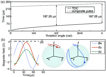
Figure 4: (color online). (a) Comparison of time costs for single-spin rotation $R^{H}_{\mathbf{n}}(\theta):=e^{-i\mathbf{n}\cdot\vec{\sigma}\frac{\theta}{2}}\otimes\mathbf{1}_{2}$ on ¹H in the ¹H-¹³C system between TOC and the composite-pulse sequence Bian2017 ; Jiang2017 implemented via $R^{H}_{\mathbf{n}}(\theta)=R^{C}_{\mathbf{n_{\bot}}}(\pi)e^{-iH(\vec{u}_{0})\tau}R^{C}_{\mathbf{n_{\bot}}}(-\pi)e^{-iH(\vec{u}_{0})\tau}$. Here $\vec{u}_{0}$ is a constant field along $\mathbf{n}$ and $\tau=\frac{\theta}{2\gamma_{1}|\vec{u}_{0}|}$. (b) Time-optimal fields and corresponding trajectories on the Bloch Sphere for realizing $R_{y}^{\textrm{H}}(\pi):=e^{-i\sigma_{y}\frac{\pi}{2}}$.

Figure 5: (color online). TOC pulses in different $\gamma$ cases. (a) TOC $\pi$ pulse on ¹³C along the $y$ axis in ¹H-¹³C. (b) TOC $\pi/2$ pulse on ¹H along the $y$ axis in ¹H-³¹P.

IV.1.2 Explicit expression of the optimal controls

We take as an example $\theta=\pi$. Using Theorem 2 we calculate the parameters ($t_{min},\omega,a,b)$ of the optimal control. We have from (26)

$$M_{\gamma}=M_{\gamma}(1,1,1,1)=\frac{5}{4}\gamma.$$ (68)

Moreover $t_{min}={\pi}\sqrt{\frac{M_{\gamma}}{\gamma(1-\gamma)}}=\frac{\pi}{2}\sqrt{\frac{5}{1-\gamma}}$. We have $\omega=\frac{\pi}{t_{min}}=2\frac{\sqrt{1-\gamma}}{\sqrt{5}}$. We have (from the Theorem)

$$a=\frac{\omega}{2\gamma}+\frac{\gamma}{2\omega}-\frac{k^{2}\pi}{2tm\gamma}=\frac{\gamma}{4}\sqrt{\frac{5}{1-\gamma}},$$

with $b=\pm\sqrt{1-a^{2}}$. With these values of $\omega,a$ and $b$, we can calculate $e^{i\omega\sigma_{z}t}(ia\sigma_{z}-ib\sigma_{y})e^{-i\omega\sigma_{z}t}$, which gives final condition (on spin 1) $\tilde{U}_{f,1}=e^{i\omega\sigma_{z}t}e^{(ia\sigma_{z}-ib\sigma_{y}-i\omega\sigma_{z})t}$ with $t=t_{min}$ (cf. (20)). In order to complete Task 6 of the procedure in subsection II.3 we need to find $Y\in\textrm{SU}(2)$ such that $U_{f,1}=Y^{\dagger}\tilde{U}_{f,1}Y$, so that $X_{1}=Y^{\dagger}e^{i\omega\sigma_{z}t}(ia\sigma_{z}-ib\sigma_{y})e^{-i\omega\sigma_{z}t}Y$, the optimal control. The optimal control fields ($u_{x},u_{y},u_{z}$) are obtained from $X_{1}=-i\sigma_{x}u_{x}-i\sigma_{y}u_{y}-i\sigma_{z}u_{z}$. If we want to consider a general bound $D$ on the control norm, we need to re-scale the optimal control which was obtained with a normalized bound ($L:=|\gamma_{1}|D=1$). The re-scaling is $\vec{u}(t)\rightarrow L\vec{u}(Lt)=|\gamma_{1}|Du(|\gamma_{1}|Dt)$. The explicit expression of the matrix $Y$ and the optimal control fields are given below. These are the control fields used in the experiment in FIG. 4.

$${Y}=\begin{pmatrix}\frac{5}{4}\sqrt{\frac{2743}{11229}}i-\frac{1}{4}\sqrt{\frac{21257}{11229}}i&\frac{5}{4}\sqrt{\frac{2743}{11229}}+\frac{1}{4}\sqrt{\frac{21257}{11229}}\cr-\frac{5}{4}\sqrt{\frac{2743}{11229}}-\frac{1}{4}\sqrt{\frac{21257}{11229}}&-\frac{5}{4}\sqrt{\frac{2743}{11229}}i+\frac{1}{4}\sqrt{\frac{21257}{11229}}i.\end{pmatrix}.$$ (69)

(we used in this calculations ratios of integer number to express $\gamma=0.2514=\frac{2514}{10000}$.) The control magnetic field $\vec{B}=(B_{x},B_{y},B_{z}):=-2(u_{x},u_{y},u_{z})\,(|\vec{B}|=2D)$ are given by

$$B_{x} \approx 1.98D\sin{(1.54D\gamma_{1}t)};$$ (70)

$$B_{y} \approx 0.18D-1.68D\cos{(1.54D\gamma_{1}t)};$$

$$B_{z} \approx-0.28D-1.04D\cos{(1.54D\gamma_{1}t)}.$$

To show the generality of the method, we have also obtained controls for different values of $\gamma$. In particular, we have considered $\frac{\gamma_{\textrm{H}}}{\gamma_{\textrm{C}}}\approx 3.9777=\gamma$, that is, the rotations are implemented on ¹³C spin in ¹H-¹³C system (now spin 1 is ¹³C and spin 2 is ¹H). In this case, $M_{\gamma}<0$ in Theorem 2 and it is $-M_{\gamma}$ that has to be minimized. We proved (like in subsection IV.1.1) that the combination $(s=-1,m=1,l=1,k=1)$ minimizes $-M_{\gamma}=M_{\gamma}(s,m,l,k)$, and the corresponding TOC $\pi$ pulse on ¹³C is illustrated in Figure 5 (a). We also considered $\gamma=0.4048$. This corresponds to a single-spin rotation on ¹H in a ¹H-³¹P system. For example, a TOC $\pi/2$ pulse on ¹H in the ¹H-³¹P system is illustrated in Figure 5 (b). In this case it is proved that the minimal $M_{\gamma}=M_{\gamma}(s,m,l,k)$ equals $M(1,1,1,1)$.

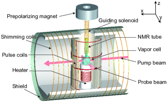
Figure 6: (color online). Schematic diagram of zero-field NMR spectrometer. The NMR sample, contained in a $5$-mm NMR tube, is detected with an atomic magnetometer with a ⁸⁷Rb vapor cell operating at $155$ ^∘C.

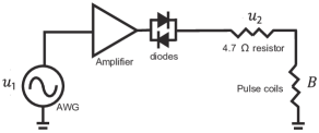
Figure 7: Pulse generation circuit. The anti-parallel diodes are placed in series with the pulse coils to isolate the noise of amplifier. The anti-parallel diodes introduce a voltage drop, which is measured in calibration experiments.

IV.2 Experimental details

TOC experiments were performed using a home-built zero-field NMR spectrometer, as illustrated in FIG. 6. Nuclear spins in the ¹³C-formic acid sample ($\approx 230~{}\mu L$) were polarized in a 1.3-T prepolarizing magnet, after which the sample was shuttled into a magnetically shielded region, such that the bottom of the sample tube is $\sim 1~{}\textrm{mm}$ above a ⁸⁷Rb vapor cell of an atomic magnetometer Allred2002 ; Budker2007 . The ⁸⁷Rb atoms in the vapor cell were pumped with a circularly polarized laser beam propagating in the $x$ direction. The magnetic fields were measured via optical rotation of linearly polarized probe laser light at the $\textrm{D}2$ transition propagating in the $y$ direction. The magnetometer was primarily sensitive to $z$ component of the nuclear magnetization, i.e., $M_{z}\propto\textrm{Tr}[\rho(t)(\gamma_{\textrm{H}}\sigma_{z}\otimes\mathbf{1}_{2}+\gamma_{\textrm{C}}\mathbf{1}_{2}\otimes\sigma_{z})]$, with a noise floor of about 15 $\textrm{fT}/\sqrt{\textrm{Hz}}$ above 100 Hz, here $\rho(t)$ is the density matrix of the ¹H-¹³C system.A guiding magnetic field ($\approx 1~{}\textrm{G}$) was applied during the transfer, and was adiabatically switched to zero after the sample reached the zero-field region. In our experiment, to ensure adiabaticity, the decay time to turn off the guiding field is 1 s. Thus the spin system is initially prepared in the adiabatic state Emondts2014 : $\rho(0)=\mathbf{1}_{4}/4+\frac{\epsilon_{\textrm{H}}+\epsilon_{\textrm{C}}}{2}(\sigma_{z}\otimes\mathbf{1}_{2}+\mathbf{1}_{2}\otimes\sigma_{z})-\frac{\epsilon_{\textrm{H}}-\epsilon_{\textrm{C}}}{4}(\sigma_{x}\otimes\sigma_{x}+\sigma_{y}\otimes\sigma_{y})$ with the polarizations $\epsilon_{\textrm{H}},\epsilon_{\textrm{C}}\sim 10^{-6}$. The TOC pulses were generated by three sets of mutually orthogonal low-inductance pulse coils, which were individually controlled by arbitrary waveform generators (Keysight 33512B with two channels, Keysight 33511B with single channel), and amplified individually with linear power amplifiers (AE TECHRON 7224) with 300 KHz bandwidth.

In FIG. 7 we present a scheme of the pulse generation circuit. FIG. 8 describes how the signal amplitude in various directions depends on the DC pulse amplitude. FIG. 9 reports an example of the experimental optimal controls’ shapes, in various directions.

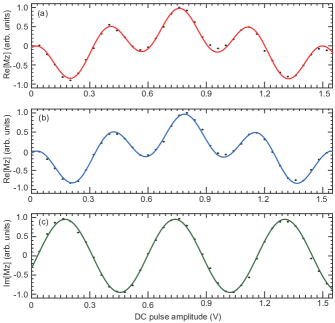
Figure 8: (color online). Dependence of signal amplitude on the DC pulse amplitude for pulses of magnetic field in the $x$ (a), $y$ (b), and $z$ (c) directions. The solid curves overlaying the data are fits to curves described in the text.

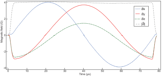
Figure 9: (color online). Experimental result of measuring TOC $\pi$ pulse. TOC $\pi$ pulse is measured by acquiring the load voltage of the resistor in series with the pulse coils.

IV.3 Performance of the TOC

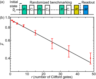
Figure 10: (color online). Randomized benchmarking (RB) experimental results. (a) RB pulse sequences. (b) RB results for ¹H single-spin TOC control. Each point $\bar{F}$ is an average over 32 random sequences of $r$ Clifford gates, and the error bars indicate the standard error of the mean. The $y$ axis is in log-scale. A single exponential decay (solid line) fits the fidelity decay and reveals an average gate fidelity of $0.99$.

To evaluate the quality of single-spin TOC control, we adopted the randomized benchmarking (RB) method Nielsen2002 ; Magesan2011 . The RB pulse sequences are shown in Fig. 10(a). The initial state is prepared as $\rho_{0}=\mathbf{1}_{4}/4+\frac{\epsilon_{\textrm{H}}}{2}\sigma_{z}\otimes\mathbf{1}_{2}+\frac{\epsilon_{\textrm{C}}}{2}\mathbf{1}_{2}\otimes\sigma_{z}$ with the polarizations $\epsilon_{\textrm{H}},\epsilon_{\textrm{C}}\sim 10^{-6}$. Random sequences with $P=e^{\pm i\frac{\pi}{2}V}\otimes\mathbf{1}_{2}$ and $C=e^{\pm i\frac{\pi}{4}Q}\otimes\mathbf{1}_{2}$ are realized by TOC control, and are applied for each sequence of length $m$, where $V\in\{\mathbf{1}_{2},\sigma_{x},\sigma_{y},\sigma_{z}\}$ and $Q\in\{\sigma_{x},\sigma_{y},\sigma_{z}\}$. The Clifford gates are realized by combined operations $PC$. The recovery gate $R$ is chosen to return the system to the initial state. To measure the coefficient of $\sigma_{z}\otimes\mathbf{1}_{2}$ independently, we adopted a recently developed state-tomography technique in zero-field NMR (see Ref. Jiang2017 ). By averaging the coefficients of $\sigma_{z}\otimes\mathbf{1}_{2}$ over 32 different RB pulse sequences with the same length $r$, and normalizing this averaged value to that of $r=0$, the normalized signal $\bar{F}$ can be fitted by $\bar{F}=(1-d_{if})(1-2\epsilon_{g})^{r}$, where $d_{if}$ is due to the imperfection of the initial state preparation and readout, and $\epsilon_{g}$ is the average gate error per Clifford gate. As shown in Fig. 10(b), the RB results yield an average gate error per Clifford gate $\epsilon_{g}=0.01$, and an imperfection of the initial state preparation and readout $d_{if}=0.05$. The average fidelity for ¹H single-spin TOC control is $f_{avg}=1-\epsilon_{g}=0.99$.

Errors in quantum control may be unitary, decoherent, and incoherent Pravia2003 . For our experiment, the most relevant is the unitary error from pulse distortion and miscalibration amplitude, caused by the bandwidth-limited pulse generation circuit, with the pulse rise/fall time $\approx 5~{}\mu s$. As the duration of TOC is shorter than that of composite pulse scheme, the rising edge will take a larger proportion in TOC pluses, hence cause more degradation in the control performance. This drawback due to the very short duration of TOC can be overcome through decreasing the total control amplitude (i.e., increasing the duration). In the future, it may be possible to correct such pulse distortion using a technique similar to the pre-distortion technique of Feng2016 . The effect of ¹H-¹³C spin-spin interaction gives an error of $\approx 5\times 10^{-4}$ per gate. The decoherent error, estimated to be $\sim 1\times 10^{-5}$ per gate, is even smaller since the coherence time of our system is substantially longer than the TOC pulse duration. The incoherent error, which mainly comes from pulse-field inhomogeneity Jiang2017 , measured to be $\sim 0.2\%$ over the sample volume, is estimated to be about $1\times 10^{-5}$ per gate.

For our ¹H-¹³C system with $\frac{\gamma_{\textrm{C}}}{\gamma_{\textrm{H}}}\approx 0.2514=\gamma$, figure 4(a) shows a $70-80\%$ time gain of TOC with respect to the composite-pulse scheme of Bian2017 ; Jiang2017 . The reason for this gain is that the schemes of Bian2017 ; Jiang2017 do not consider time optimality. Moreover they use control fields in two directions only rather than three.

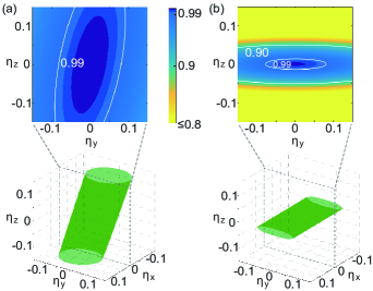
Figure 11: (color online). Robustness tests of TOC and composite pulse scheme with respect to pulse imperfections. The amplitude distortion ratio in $k=x,y,z$ is defined as $\eta_{k}=\frac{\textrm{amplitude distortion in k}}{\textrm{ideal value in k}}$. Lower figures in (a), (b) show the isosurface of $\textrm{fidelity}=0.99$ for TOC and composite pulse, respectively. Upper figures in (a), (b) are the fidelity contour maps for these two methods. The better fidelity of TOC is indicated by the larger area with a fidelity higher than $0.99$.

IV.4 Robustness of the optimal control law

Once the optimal control problem is solved with a bound $L$ on the control and $t_{\textrm{min}}$, the number $Lt_{\textrm{min}}$ is independent of $L$ and it gives the sub-Riemannian distance $d$ of the final condition $U_{f,1}\otimes U_{f,1}$ from the identity, $d:=d(U_{f,1}\otimes U_{f,2})$. According to Chow-Rashevskii theorem (see, e.g., ABB ) such a distance is equivalent to the given metric on the manifold (in this case $\textrm{SU}(2)\otimes\textrm{SU}(2)$). From a practical point of view it is interesting to investigate how robust the control law is with respect to the variations in the parameters of the model, in particular the parameter $\gamma$. Assume for instance that the gyromagnetic ratio $\gamma_{1}$ is known with some confidence while $\gamma_{2}$, and therefore $\gamma$ is known with less confidence. From Theorem 1 it follows that the final value on the first spin is independent of $\gamma$ while the error is all on the final state of the second spin. Differentiating the operation $U_{2}$ of Theorem 1, i.e., the operation on the second spin, with respect to $\gamma$ we obtain (for $U_{2}=U_{f,2}$, the desired final condition)

$$\frac{dU_{f,2}}{d\gamma}=e^{At_{\textrm{min}}}Pt_{\textrm{min}}e^{-At_{\textrm{min}}}U_{f,2},$$ (71)

so that (assuming because of unitarity $\|U_{f,2}\|=1$), $\|\frac{dU_{f,2}}{d\gamma}\|\leq\|e^{At_{\textrm{min}}}Pt_{\textrm{min}}e^{-At_{\textrm{min}}}\|=|P|t_{\textrm{min}}:=Lt_{\textrm{min}}=d(U_{f,1}\otimes U_{f,2})$. Therefore, the sensitivity with respect to $\gamma$ of the final condition is bounded by the sub-Riemannian distance of the desired final condition. From simulation, a $1\%$ deviation in $\gamma$ will only result in a $0.001\%$ drop in fidelity (for the TOC used in this experiment).

The robustness of TOC against distortions in control fields is also demonstrated in Figure 11. Even in this regard, the TOC is preferable as compared to composite pulse scheme.

V Conclusion and discussion

We have theoretically derived and experimentally demonstrated, the time optimal control of two independent spin-$\frac{1}{2}$ particles by simultaneous control. Novel techniques of symmetry reduction allowed us to obtain analytic expressions of the TOC, with minimal use of numerical experiments. Such control fields, implemented using a zero-field heteronuclear NMR system, gave an average fidelity of $99\%$, and considerable time saving. Our paper adds to the recently growing literature that combines analytical methods with experimental implementations in quantum mechanical control Geng2016 , KhanP1 , KhanP2 , KhanP3 , Avinadav2014 , glaserpraref .

Typical optimal control techniques and applications to quantum systems use numerical methods which involve the repeated numerical integration of a system of differential equations with variable initial conditions (parameters). In our case, there is no need of numerical integration since the solution is given in explicit form. Moreover the number of parameters is reduced to a minimum with the technique of symmetry reduction. Still computer experiments can be a useful tool to solve the Task 3 of the procedure in section II.3 by visualizing the reachable set in the quotient space and-or by helping in the solution of integer optimization problems, such as the one described in Theorem 2.

Ideas presented here can be applied more in general for quantum systems displaying symmetries such as the $KP$ systems considered in Albertini2018 . The analytic knowledge of the TOC is useful even in cases where such a control is not the one physically implemented. It gives information about the inherent time limitations of the system, therefore indicating a benchmark for the time of any control law. The knowledge of the TOC law for any final condition is also equivalent to a description of the reachable sets which, in the presence of symmetries, can be carried out in the (reduced) orbit space Albertini2018 .

It is interesting to investigate whether the optimal control techniques discussed here can be scaled to higher dimensional systems and in particular in the simultaneous control of $N>2$ spin $\frac{1}{2}$ systems. In general, optimal control problems become harder as the dimension of the system increases with respect to the number of controls. More specifically, the main reason why we were able to find an explicit form for the optimal control and trajectory for our system is the fact that the system has degree of non-holonomy one, that is, it is enough to do one Lie bracket of the vector fields which appear in the Schrödinger equation to obtain the whole Lie algebra of available directions of motion. This property is lost if we increase the number of spins and keep the number of control fixed. It maybe recovered if we introduce additional controls by, for example, assuming that $N/2$ systems each consisting of two spin $\frac{1}{2}$’s can be controlled independently. Under these assumptions, one may use techniques similar to the ones considered in Domenico1 , Domenico2 for the case of $N/2$ systems each consisting of one spin only. Such controls and optimal times still give lower bounds on the time of transfer in more realistic scenarios with fewer controls.

Acknowledgment.–We thank X. Rong and A. Voronov for valuable discussions. Support came from National Key Research and Development Program of China (Grant No. 2018YFA0306600), National Key Basic Research Program of China (Grant No. 2014CB848700), National Natural Science Foundation of China (Grants Nos. 11425523, 11375167, 11661161018, 11227901), Anhui Initiative in Quantum Information Technologies (Grant No. AHY050000), National Science Foundation (Grant ECCS 1710558).

Y. J., J. B., and M. J. contributed equally to this work.

VI appendix

VI.1 Proof of Proposition II.2

Proof. We first have to show that the map (21) is well defined, i.e., it does not depend on the choice of the representative $(U,Z)$ in $[(U,Z)]$ nor on the choice of $S$ when writing $U$ as $U=S\Lambda S^{\dagger}$ in (22). Let us show the latter property first. If $U=S_{1}\Lambda S_{1}^{\dagger}=S_{2}\Lambda S_{2}^{\dagger}$ then $S_{1}^{\dagger}S_{2}$ commutes with $\Lambda$ and since $\Lambda$ is not $\pm{\bf 1}$ then $S_{1}^{\dagger}S_{2}$ must be a diagonal matrix. This implies that we must have $(S_{1}^{\dagger}ZS_{1})_{1,1}=(S_{2}^{\dagger}ZS_{2})_{1,1}$. Consider now (22). Assume that instead of $(U,Z)$ we take the representative $(FUF^{\dagger},FZF^{\dagger})$, in $[(U,Z)]$ for some $F\in SU(2)$. Write $FUF^{\dagger}:=FS\Lambda S^{\dagger}F^{\dagger}$. This gives the same value of $\phi$ and it does not change the $(1,1)$ entry of $(S^{\dagger}F^{\dagger})FZF^{\dagger}(FS)=S^{\dagger}ZS$. Analogously in the case (23) and (24) a similarity transformation does not modify the eigenvalues of $X$ and $Z$.

It is clear that the map $\Psi$ is onto. To show that it is one to one assume that $\Psi([(U_{1},Z_{1})])=\Psi([(U_{2},Z_{2})])$. Then the eigenvalues of $U_{1}$ and $U_{2}$ are the same. If $U_{1}$ and $U_{2}$ are both $\pm{\mathbbm{1}}$ then the eigenvalues of $Z_{1}$ and $Z_{2}$ must be the same, and so there exists an $F\in\textrm{SU}(2)$ such that $Z_{2}=FZ_{1}F^{\dagger}$. If $U_{1}$, and therefore $U_{2}$, is different from $\pm{\mathbbm{1}}$, they have however the same eigenvalues. So there exist $S_{1},S_{2}\in\textrm{SU}(2)$ such that $U_{1}=S_{1}\Lambda S_{1}^{\dagger}$ $U_{2}=S_{2}\Lambda S_{2}^{\dagger}$. Moreover $S_{1}^{\dagger}Z_{1}S_{1}$ and $S_{2}^{\dagger}Z_{2}S_{2}$ have the same $(1,1)$ entry. So they only differ by similarity transformation by a diagonal matrix $H_{d}$ and we have $S_{2}^{\dagger}Z_{2}S_{2}=H_{d}S_{1}^{\dagger}Z_{1}S_{1}{H_{d}}^{\dagger}$, from which

$$Z_{2}=S_{2}H_{d}S_{1}^{\dagger}Z_{1}S_{1}{H_{d}}^{\dagger}S_{2}^{\dagger}.$$ (72)

By writing $U_{1}=S_{1}\Lambda S_{1}^{\dagger}$ as $U_{1}=S_{1}{H_{d}}^{\dagger}\Lambda{H_{d}}S_{1}^{\dagger}$ and from $U_{2}=S_{2}\Lambda S_{2}^{\dagger}$, we obtain

$$U_{2}=S_{2}{H_{d}}S_{1}^{\dagger}U_{1}S_{1}{H_{d}}^{\dagger}S_{2}^{\dagger}.$$ (73)

Comparing (72) and (73), we have that $[(U_{1},Z_{1})]=[(U_{2},Z_{2})]$.

VI.2 Some useful computations

We report here the results of some computations, in particular the exponential of matrices, which are useful in the process of determining the optimal control. We first calculate the exponential $e^{Ft}$ with

$$F:=ic\sigma_{z}-id\sigma_{y}=\begin{pmatrix}ic&-d\cr d&-ic\end{pmatrix}.$$ (74)

We have

$$e^{Ft}=\begin{pmatrix}\cos(\sqrt{c^{2}+d^{2}}t)+i\frac{c}{\sqrt{c^{2}+d^{2}}}\sin(\sqrt{c^{2}+d^{2}}t)&-\frac{d}{\sqrt{c^{2}+d^{2}}}\sin(\sqrt{c^{2}+d^{2}}t)\cr\frac{d}{\sqrt{c^{2}+d^{2}}}\sin(\sqrt{c^{2}+d^{2}}t)&\cos(\sqrt{c^{2}+d^{2}}t)-i\frac{c}{\sqrt{c^{2}+d^{2}}}\sin(\sqrt{c^{2}+d^{2}}t)\end{pmatrix}.$$ (75)

This formula can be used to compute $\tilde{U}_{1}(t)$ and $\tilde{U}_{2}(t)$ in (20) by using, for the second factor of

$$\tilde{U}_{1}=e^{i\omega\sigma_{z}t}e^{(ia\sigma_{z}-ib\sigma_{y}-i\omega\sigma_{z})t}=e^{i\omega\sigma_{z}t}e^{[i(a-\omega)\sigma_{z}-ib\sigma_{y}]t},$$ (76)

$$c:=a-\omega,\qquad d:=b,$$ (77)

and, for the second factor of

$$\tilde{U}_{2} =e^{i\omega\sigma_{z}t}e^{(i\gamma a\sigma_{z}-i\gamma b\sigma_{y}-i\omega\sigma_{z})t}$$ (78)

$$=e^{i\omega\sigma_{z}t}e^{[i(\gamma a-\omega)\sigma_{z}-i\gamma b\sigma_{y}]t},$$

$$c:=\gamma a-\omega,\qquad d:=\gamma b.$$ (79)

Let us consider the case of $\tilde{U}_{2}$ since the case of $\tilde{U}_{1}$ can be recovered by setting $\gamma=1$. In this case, a simple calculation using the fact that $a^{2}+b^{2}=1$ and formulas (79) gives

$$\sqrt{c^{2}+d^{2}} =\sqrt{(\gamma a-\omega)^{2}+\gamma^{2}\left(1-a^{2}\right)}$$ (80)

$$=\sqrt{\omega^{2}+\gamma^{2}-2a\omega\gamma}:=\eta_{\gamma}:=\eta_{\gamma}(a,\omega).$$

Let us assume $|a|<1$ so that $\eta_{1}\not=0$ and, in general, $\eta_{\gamma}\not=0$ for any $\gamma$. Then using (75), we have for $\tilde{U}_{1}$ in (76)

$$\tilde{U}_{1}(t):=\begin{pmatrix}e^{i\omega t}(\cos(\eta_{1}t)+i\frac{a-\omega}{\eta_{1}}\sin(\eta_{1}t))&-e^{i\omega t}\frac{b}{\eta_{1}}\sin(\eta_{1}t)\cr e^{-i\omega t}\frac{b}{\eta_{1}}\sin(\eta_{1}t)&e^{-i\omega t}(\cos(\eta_{1}t)-i\frac{a-\omega}{\eta_{1}}\sin(\eta_{1}t))\end{pmatrix}.$$ (81)

Also, still when $|a|<1$, using (75), we have for $\tilde{U}_{2}$ in (78)

$$\tilde{U}_{2}(t):=\begin{pmatrix}e^{i\omega t}(\cos(\eta_{\gamma}t)+i\frac{\gamma a-\omega}{\eta_{\gamma}}\sin(\eta_{\gamma}t))&-e^{i\omega t}\frac{\gamma b}{\eta_{\gamma}}\sin(\eta_{\gamma}t)\cr e^{-i\omega t}\frac{\gamma b}{\eta_{\gamma}}\sin(\eta_{\gamma}t)&e^{-i\omega t}(\cos(\eta_{\gamma}t)-i\frac{\gamma a-\omega}{\eta_{\gamma}}\sin(\eta_{\gamma}t)),\end{pmatrix}$$ (82)

VI.3 Solution of the Optimization Problem of Theorem 2 for the case $\gamma=1/2$

Consider $\gamma=\frac{1}{2}$ and $\theta=\pi$ ($q=1$). The desired evolution is

$$U_{f,1}=\pm\textrm{Phase}=\pm\begin{pmatrix}-i&0\cr 0&i\end{pmatrix},\quad U_{f,1}=\pm\begin{pmatrix}1&0\cr 0&1\end{pmatrix}$$ (83)

With $\theta=\pi$, (33) can be simplified to

$$m\sqrt{\omega^{2}+1-2a\omega}\,t=\frac{{l}\pi}{2},\quad$$ (84)

where $l$ can only be an odd positive integer. Thus the cases with $s=\pm 1$ can be combined, and (26) becomes

$$M(m,l,k):=m^{2}(1-\gamma)+\frac{l^{2}}{4}\gamma-k^{2},$$ (85)

with the constraint (41) simplified to

$$\left(m-\frac{l}{2}\right)^{2}<\frac{M(m,l,k)}{\gamma(1-\gamma)}<\left(m+\frac{l}{2}\right)^{2}.$$ (86)

Using (85) and (86), we obtain the condition

$$\left(m-\frac{l}{2}\right)^{2}<4k^{2}<\left(m+\frac{l}{2}\right)^{2}.$$ (87)

Given $M_{\gamma}$ in (85), (37), and the fact that $\gamma(1-\gamma)$ is positive in this case, we need to find the largest possible $k$ which satisfies (87) in terms of $l$ and $m$. If we define $\tilde{s}:=2m+l$, the largest possible $k$ which satisfies the right inequality in (87) is (recall $l$ is odd so $\tilde{s}=2m+l$ is also odd)

$$k=\frac{\tilde{s}-1}{4},\qquad\texttt{for}\qquad\tilde{s}=5,9,13,...,$$ (88)

and

$$k=\frac{\tilde{s}-3}{4},\qquad\texttt{for}\qquad\tilde{s}=7,11,15,...$$ (89)

The case $\tilde{s}=3$ is not possible since $k\not=0$. Also with this choice of $k$ the left inequality in (87) is always satisfied unless $l=1$ and $m$ is odd. In the latter case, since $k$ in (89) and (88) is the largest possible value, no other value of $k$ would satisfy the left inequality in (87). Thus, the values $l=1$ and $m$ odd are excluded from the search. Replacing $k$ in (85), with $\gamma=\frac{1}{2}$, we obtain

$$\frac{M}{\gamma(1-\gamma)} =2m^{2}+\frac{l^{2}}{2}-4k^{2}=\frac{1}{2}(2m+l)^{2}-4k^{2}-2ml$$ (90)

$$=\frac{\tilde{s}^{2}}{2}-\frac{(\tilde{s}-h)^{2}}{4}-2m(\tilde{s}-2m)$$

$$=\frac{\tilde{s}^{2}}{4}-\frac{(\tilde{s}-h)^{2}}{4}+\left(2m-\frac{\tilde{s}}{2}\right)^{2},$$

where $h=1$ or $h=3$ if we are in case (88) and (89) respectively. For a given $s$ the minimum in (90) is given for $m=\frac{\tilde{s}-h}{4}$, and it is given by

$$\frac{M}{\gamma(1-\gamma)}=\frac{h\tilde{s}}{2},$$ (91)

which is minimized with $\tilde{s}=5$ ($h=1$). We have therefore the following optimal values for $m$, $l$ and $k$ (with $\tilde{s}=5$ and $h=1$):

$$m=\frac{\tilde{s}-h}{4}=1,\ l=\tilde{s}-2m=3,\ k=\frac{\tilde{s}-h}{4}=1.$$ (92)

References

• (1) M. Shapiro and P. Brumer, Principles of the Quantum Control of Molecular Processes, (Wiley, New Jersey, 2003).
• (2) T. Schulte-Herbr$\ddot{\textrm{u}}$ggen, A. Sp$\ddot{\textrm{o}}$rl, N. Khaneja, and S. J. Glaser, Phys. Rev. A 72, 042331 (2005).
• (3) R. R. Ernst, Principles of Nuclear Magnetic Resonance in One and Two Dimensions, (Oxford University Press, Oxford, 1990).
• (4) S. J. Glaser, U. Boscain, T.Calarco, C. P. Koch, W. Kockenberger, R. Kosloff, I. Kuprov, B. Luy, S. Schirmer, T. S. Herbruggen, D.Sugney, F. K. Wilhelm, Eur. Phys. J. D 69, 279 (2015)
• (5) A. Carlini, A. Hosoya, T. Koike, and Y. Okudaira, Phys. Rev. Lett. 96, 060503 (2006).
• (6) A. T. Rezakhani, W.-J. Kuo, A. Hamma, D. A. Lidar, and P. Zanardi, Phys. Rev. Lett. 103, 080502 (2009).
• (7) X. Wang, M. Allegra, K. Jacobs, S. Lloyd, C. Lupo, and M. Mohseni, Phys. Rev. Lett. 114, 170501 (2015).
• (8) J. Geng, Y. Wu, X. Wang, K. Xu, F. Shi, Y. Xie, X. Rong, and J. Du, Phys. Rev. Lett. 117, 170501 (2016).
• (9) Y. L. Sachkov, Lecture notes SISSA, 15 (2006).
• (10) A. Rao, Adv. Astronaut. Sci. 135, (2010).
• (11) Q. Chen, R. Wu, T. Zhang, and H. Rabitz, Phys. Rev. A 92, 063415 (2015).
• (12) N. Khaneja, S. J. Glaser, and R. Brockett, Phys. Rev. A 65, 032301 (2002).
• (13) H. Yuan and N. Khaneja, Phys. Rev. A 72, 040301 (2005).
• (14) F. Albertini, D. D’Alessandro, J. Dyn. Control. Syst. 24, 13 (2018).
• (15) J. W. Blanchard and D. Budker, eMagRes 5, 1395 (2016).
• (16) J. Bian et al., Phys. Rev. A 95, 052342 (2017).
• (17) M. Jiang et al., Sci. Adv. 4, 6 (2018).
• (18) R. Romano, Phys. Rev. A 90, 062302 (2014).
• (19) D. D’Alessandro, Introduction to Quantum Control and Dynamics, (CRC, Boca Raton FL, 2007).
• (20) U. Boscain, T. Chambrion, and J.P. Gauthier, J. Dyn. Control. Syst. 8, 4 (2002).
• (21) A pair $(X,U)$ satisfying the conditions of the PMP is called an extremal, i.e., an optimal candidate. It is called a normal extremal if $\lambda_{0}\not=0$, abnormal if $\lambda_{0}=0$. It follows from the analysis of (1) that abnormal extremals cannot be optimal since the Goh condition (see, e.g., Appendix C in OptRes and references therein) is not verified for them. Normalcy of the optimal control implies, from known results in sub-Riemannian geometry, that the optimal trajectory $U=U(t)$ and therefore the optimal control $X=X(t)$ is $C^{\infty}$ as a function of $t$ ABB . In our case, it is, in fact, analytic since the system is analytic Suss2 .
• (22) H. J. Sussmann, Proceedings of the 53rd IEEE Conference on Decision and Control (2014).
• (23) It is a general fact that in driftless TOC problem such as the one considered here the bound $|\vec{u}|\leq D$, a.e., is equivalent to $|\vec{u}|=D$. A formal proof of this fact is given in Albertini2018 .
• (24) This is the space of equivalence classes in $SU(2)\otimes SU(2)$ where $Z_{1}$ is equivalent to $Z_{2}$ if and only if there exists a $\tilde{Y}\in G$ such that $\tilde{Y}Z_{1}\tilde{Y}^{\dagger}=Z_{2}$.
• (25) This result was proved in collaboration with A. Voronov at the School of Mathematics, University of Minnesota
• (26) $W_{1},W_{2}\neq\pm\mathbf{1}_{2}$.
• (27) N. Khaneja, R. Brockett and S. J. Glaser, Phys. Rev. A 63, 032308 (2001).
• (28) S. Helgason, Differential geometry, Lie groups and symmetric spaces, (Academic Press, New York, 1978).
• (29) J. Sniatycki, Differential Geometry of Singular Spaces and Reduction of Symmetry, (Cambridge University Press, 2013).
• (30) F. Albertini and D. D’Alessandro, Automatica, 74, December 2016, pp. 55-62.
• (31) M. Emondts, M. P. Ledbetter, S. Pustelny, T. Theis, B. Patton, J. W. Blanchard, M. C. Butler, D. Budker, and A. Pines, Phys. Rev. Lett. 112, 077601 (2014).
• (32) J. C. Allred, R. N. Lyman, T. W. Kornack, and M. V. Romalis, Phys. Rev. Lett. 89, 130801 (2002).
• (33) D. Budker, and M. Romalis, Nat. Phys. 3, 227 (2007).
• (34) M. A. Nielsen, Phys. Lett. A 303, 249 (2002).
• (35) E. Magesan, J. M. Gambetta, and J. Emerson, Phys. Rev. Lett. 106, 180504 (2011).
• (36) M. A. Pravia et al., J. Chem. Phys. 119, 9993 (2003).
• (37) G. Feng et al., Phys. Rev. Lett. 117, 260501 (2016).
• (38) A. Agrachev, D. Barilari and U. Boscain, Lecture notes SISSA (2011).
• (39) T. O. Reiss, N. Khaneja, and S. J. Glaser, J. Magn. Reson. 154, 2, (2002).
• (40) N. Khaneja, F. Kramer and S. J. Glaser, J. Magn. Reson. 173, 1, (2005).
• (41) N. Khaneja, B. Heitmann, A. Spörl, H. Yuan, T. Schulte-Herbruggen and S. J. Glaser, Phys. Rev. A 75, 012322 (2007).
• (42) C. Avinadav, R. Fischer, P. London, D. Gershoni, Phys. Rev. B 89, 245311 (2014).
• (43) E. Assemat, M. Lapert, Y.Zhang, M.Braun, S.J.Glaser, D.Sugny, Phys. Rev. A 82, 013415 (2010).
• (44) F. Albertini and D. D’Alessandro, IEEE Trans. Autom. Control 99, (2017).