Policy Gradient in Partially Observable Environments:
Approximation and Convergence

Abstract

Policy gradient is a generic and flexible reinforcement learning approach that generally enjoys simplicity in analysis, implementation, and deployment. In the last few decades, this approach has been extensively advanced for fully observable environments. In this paper, we generalize a variety of these advances to partially observable settings, and similar to the fully observable case, we keep our focus on the class of Markovian policies. We propose a series of technical tools, including a novel notion of advantage function, to develop policy gradient algorithms and study their convergence properties in such environments. Deploying these tools, we generalize a variety of existing theoretical guarantees, such as policy gradient and convergence theorems, to partially observable domains, those which also could be carried to more settings of interest. This study also sheds light on the understanding of policy gradient approaches in real-world applications which tend to be partially observable.

1 Introduction

Reinforcement learning (RL) is the study of sequential decision making under uncertainty with a vast application in real-world problems such as robotics, ad-allocation, recommendation, and autonomous vehicles systems. In RL, a decision-making agent interacts with its surrounding environment, collects experiences throughout the interaction, and develops its understanding of the environment. The agent exploits this information to improve its behavior and strategies for further exploration. One of the main problems in RL is the design of efficient algorithms that improve the agent’s performance in high dimensional environments and maximize a notion of reward.

Recent advances in RL, particularly in deep RL (DRL), have shown major enhances in high-dimensional RL problems. Among the most popularized ones, Abbasi-Yadkori and Szepesvári (2011) addresses control in linear systems, Mnih et al. (2015) proposes Deep-Q networks and tackles arcade games (Bellemare et al., 2013), Silver et al. (2016) uses upper confidence bound tree search (Kocsis and Szepesvári, 2006) and tackles board games, and Schulman et al. (2015) employs policy gradient (PG) (Aleksandrov et al., 1968) and addresses continuous control problems, especially MuJoCo (Todorov et al., 2012) environments.

This paper is concerned with PG methods, which are among the prominent methods in high-dimensional RL. PG methods are gradient optimization-based, and mainly approach RL as stochastic optimization problems. These methods usually deploy Monte Carlo sampling to estimate the gradient updates, resulting in high variance gradient estimations (Rubinstein, 1969). Recent works study Markov decision processes (MDP) and exploit the MDP structure to mitigate this high variance issue (Sutton et al., 2000; Kakade and Langford, 2002; Kakade, 2002; Schulman et al., 2015; Lillicrap et al., 2015). These works employ value-based methods, and provide low variance PG methods, mainly in infinite horizon discounted reward MDPs, and pave the road to guarantee monotonic improvements in the performance (Kakade and Langford, 2002). However, they do not offer optimality guarantees.

Understanding the convergence characteristics of PG methods, along with their global optimality properties, and relationship with problem-specific dependencies, are essential for effective algorithm design in real-world applications. Recently, a study by Fazel et al. (2018) advances the understanding of the optimization landscape of the infinite horizon linear quadratic problems and proposes a set of algorithms which are guaranteed to converge to the optimal control under a coverage assumption. Further encouraging studies provide convergence analyses of PG related methods in MDPs mainly using fixed-point convergence arguments (Liu et al., 2015; Bhandari and Russo, 2019; Agarwal et al., 2019; Wang et al., 2019; Abbasi-Yadkori et al., 2019). These analyses advance the understating of PG methods related in infinite-horizon MDPs.

These recent developments of PG methods, both theoretical and empirical, are confined to fully observable setting MDPs. However, in many real-world RL applications, e.g., robotic, drone delivery, and navigation, the underlying states of the environments are hidden, i.e., they are more appropriately modeled as partially observable MDPs. In POMDPs, the observation process need not be Markovian, and only incomplete information of the underlying state of the environment is accessible to the decision-makers.

In this work, we theoretically study PG methods in episodic POMDPs, and analyze their convergence properties and optimality guarantees. We establish these results for both discounted and undiscounted reward scenarios. We also develop a series of PG algorithms, agnostic to the underlying environment model, fully (MDPs), or partially observable (POMDPs). To design algorithms that are agnostic to the choice of the underlying model, we adopt the class of Markovian policies (Puterman, 2014), which, under certain regularity conditions, are optimal for MDPs. We propose a series of technical tools, including a novel notion of advantage function along with value and Q functions for POMDPs, that we employ to analyze PG methods.

We analyze and generalize a range of MDP methods to the POMDP setting, such as trust region policy optimization (TRPO) (Schulman et al., 2015), and proximal policy optimization (PPO) (Schulman et al., 2017). The resulting generalized TRPO (GTRPO) and generalized PPO (GPPO) methods are among the few for POMDPs that are computationally feasible. We conclude our study by showing how the tools developed in this work make it feasible to generalize a variety of existing MDP based advanced algorithms to POMDPs. This study sheds light on the understanding of PG approaches in real-world applications that are inherently partially observable.

Extended motivation, problem setting, and contribution.

In the following, we provide a detailed introduction of the setting of study in this paper, explain hardness results, and conclude with a detailed explanation of our contributions. Table 1 categorizes the majority of the RL paradigm concerning their observability, policy class, horizon, and discounting factor.

Table 1: While the majority of the prior works study MDPs and Markovian policies under discounted reward and infinite horizon considerations, we focus our study on episodic problems, no matter MDP or POMDP, Markovian or non-Markovian, and discounted or undiscounted.

Observability	Policy Class	Discounting	Horizon
MDP	Markovian	Discounted	Infinite
POMDP	non-Markovian	Undiscounted	Episodic

Episodic and infinite horizon: Many contemporary applications of RL are cast as episodic and/or finite horizon problems. Episodic RL refers to settings where learning happens iteratively over episodes, with each episode comprising running the current policy from a (often fixed) distribution of initial states, collecting data, and updating the policy. Episodic RL is thus appropriate for any sequential decision making tasks that are run in a repeated fashion. Infinite horizon refers to casting the problem as running each episode over for infinite time steps. Episodic, finite-horizon test-bed environments, such as MuJoCo, have played a major role in the recent empirical successes of algorithm design in RL, despite many of those algorithms being designed for the infinite horizon setting. While the study of infinite horizon environments is an essential topic of research, we dedicate this paper to episodic environments.

Discounted and undiscounted reward: Another distinction, is whether to use discounted or undiscounted cumulative rewards. In the discounted cumulative reward settings, rewards that are received earlier in time are more favorable to those received later in time. In this setting, discounted cumulative rewards are accumulations of rewards that are (typically exponentially) discounted through time. In contrast, in the undiscounted cumulative reward settings, RL agents are indifferent to when a unit of reward is received, as long as it is received. In repetitive related tasks with a clear completion goal (e.g., cooking), we might be interested in the episodic undiscounted reward with fixed horizons. In such tasks, we might be concerned with task accomplishment in a fixed period of time. In contrast, long-horizon tasks with accumulated goals, such as vacuuming, we might rather have a given physical area to be cleaned earlier than later without specifically specifying a task horizon. Discounted rewards also favor completing tasks early rather than later, owing to putting lower weight on rewards in future time steps. While the previous theoretical development of PG methods  (Schulman et al., 2015; Lillicrap et al., 2015) are mainly dedicated to the discounted reward setting (also infinite horizon), we extend our study to both the discounted and undiscounted reward settings.

Fully and partially observable: While PG can in principle be applied very generically, as mentioned above, previous research on advanced PG methods has larged focused on (fully observable) MDPs. Many real-world learning and decision-making tasks, however, are inherently partially observable where an incomplete representation of the state of the environment is accessible. Owing to the inability to directly observe the (latent) underlying states, learning in POMDP environments poses significant challenges and also adds computational complexity to the resulting policy optimization problem. Moreover, it is known that applying MDP based methods on POMDPs can result in policies with arbitrarily bad expected returns (Williams and Singh, 1999; Azizzadenesheli et al., 2017). In this work, we study environment agnostic PG methods and provide convergence as well as monotonic improvement guarantees for both MDPs and POMDPs.

Markovian and non-Markovian policies: Under a few conditions (Puterman, 2014), for any given MDP, there exists an optimal policy which is deterministic and Markovian (that maps the agent’s immediate or current observation of the environment to actions). In contrast, when dealing with POMDPs, we might be interested in the class of non-Markovian and history-dependent policies (that map the state-action trajectory history to distributions over actions). However, tackling non-Markovian and history-dependent policies can be computationally undecidable (Madani et al., 1999) for the infinite horizon, or PSPACE-Complete (Papadimitriou and Tsitsiklis, 1987) in the finite-horizon POMDPs. To avoid undesirable computational burdens, we focus on Markovian policies.

Indeed, many prior works study Markovian policies for POMDPs (Baxter and Bartlett, 2001; Littman, 1994; Baxter and Bartlett, 2000; Azizzadenesheli et al., 2016) where, in general, the optimal policies are stochastic (Littman, 1994; Singh et al., 1994; Montufar et al., 2015). Acknowledging the computation complexity of Markovian policies (Vlassis et al., 2012), this line of work highlights the broad interest, importance, and applicability of Markovian policies.

We are further interested in algorithms that are agnostic to the underlying model, as restricting to such algorithm designs can also avoid certain undesirable computational burdens. We do so by choosing Markovian policies, which are generally optimal for MDPs. This choice of the policy class allows us to use that same class of functions to represent policies in POMDPs. We can thus carry over PG results from MDPs directly to their POMDP counterparts. An additional practical advantage is that it is straightforward to re-purpose well-developed software implementations of MDP-based PG algorithms for the POMDP setting.

One could alternatively consider history-dependent policies, which is a richer function class than Markovian policies. However, utilizing history-dependent policies requires turning a given POMDP problem to a potentially non-stationary MDP with states as concatenations of the historical data. As such, a thorough theoretical treatment of history-dependent policies for POMDPs would likely require leveraging theoretical analyses for non-stationary MDPs.

Equivalence policy classes and the role of observation boundary: The expressiveness of general policy classes is mainly entangled with the definition of the observation. Under some regularity conditions, for any given class of history-dependent policies on a POMDP, there exists a class of Markovian policies on a new POMDP such that: $(1)$ the observations of the new POMDP are the (typically) discrete concatenations of the historical data in the former POMDP; and $(2)$ the two policy classes are equivalent, i.e., the respective policies result in the same behavior (e.g., action sequence). In other words, instead of making the policies non-Markovian and history-dependent, we can keep them Markovian and instead enrich the observation space. Similarly, for any limited-memory policy class (depending on a fixed window of history instead of the whole history, e.g., the policies in MDPs of order more than one), there is an enrichment of the observation that results in an equivalent class of Markovian policies. This observation-enrichment viewpoint is known as the emergentism approach. In essence, these distinctions boil down to: “What a Markovian policy is Markovian with respect to”.

The above reasoning implies that, by considering the class of Markovian policies in episodic POMDPs, we often will not restrict the generality of the results in this paper. Therefore, despite focusing on Markovian policies, our results also hold for both classes of limited-memory as well as history-dependent policies through representing histories as observations.

Detailed Summary of Contributions. In this paper, we study Markovian policies in episodic POMDPs and MDPs, with both discounted and discounted rewards.

$(i)$ We state the general PG theorems in the POMDP framework. These theorems are based on are well-known theorems that make no specific modeling assumption on the underlying environments. We extend the value-based PG theorems on MDP, such as deterministic PG (Silver et al., 2014), to POMDPs. While the extensions are straightforward, we provide them for clarity and completeness.

$(ii)$ We define a novel notion of advantage function for POMDPs and advance a series of MDP-based theoretical results to POMDPs. In MDPs, the advantage functions are well defined, and they are functions of one event (i.e., one state-action pair). However, the states in POMDPs are partially observed, and the classical definition of advantage functions does not directly carry to partially observable cases. For POMDPs, our advantage function depends on three consecutive events instead of just one. Utilizing this definition, we generalize the policy improvement guarantees in MDPs (Kakade and Langford, 2002; Schulman et al., 2015) to POMDPs. Note that conditioning on three consecutive events for learning in POMDPs matches the results in Azizzadenesheli et al. (2016), which indicate that the statistics of three consecutive events are sufficient to learn POMDP dynamics and guarantee order-optimal sample complexity properties of Markovian policies.

$(iii)$ We study how to extend natural policy gradient methods for MDPs to POMDPs. This derivation leverages our novel notion of advantage function.

$(iv)$ We propose generalized trust region policy optimization (GTRPO) PG methods, as a generalization of  Kakade and Langford (2002); Schulman et al. (2017) to the general classes of episodic MDPs and POMDPs under both discounted and undiscounted reward settings. GTRPO utilize the property of newly developed advantage function, and computes a low variance estimation of the PG updates. We then construct a trust region for the policy search step in GTRPO and show that the policy updates of GTRPO are guaranteed to monotonically improve the expected return. GTRPO is among the few methods for POMDPs that are computationally feasible.

$(v)$ We propose generalized proximal policy optimization (GPPO), a generalization of the PPO algorithm (Schulman et al., 2017) to the general classes of episodic MDPs and POMDP under both discounted and undiscounted reward settings. GPPO is an extension to GTRPO, as PPO is an extension of TRPO, which is known to be computation more efficient than its predecessor.

We conclude the paper by stating that the developed machinery in this paper, can be used to extend a variety of existing MDP-based methods directly to their general POMDP cases.

2 Preliminaries

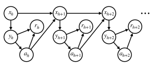
Figure 1: POMDP under a Markovian policy

An episodic stochastic POMDP, $M$, is a tuple $\langle\mathcal{X},\mathcal{A},\mathcal{Y},P_{1},T,R,O,\gamma,x_{Terminal}\rangle$ with a set of latent states $\mathcal{X}$, observations $\mathcal{Y}$, actions $\mathcal{A}$, and their elements denoted as $x\in\mathcal{X}$, $y\in\mathcal{Y}$, and $a\in\mathcal{A}$, accompanied with a discount factor $0\leq\gamma\leq 1$. Under reasonable assumptions, let $P_{1}(\cdot):\mathcal{X}\rightarrow[0,\infty]$ represent the probability distribution of the initial latent states, $T(\cdot|\cdot,\cdot):\mathcal{X}\times\mathcal{X}\times\mathcal{A}\rightarrow[0,\infty]$ denotes the transition kernel on the latent states, $O(\cdot|\cdot):\mathcal{Y}\times\mathcal{X}\rightarrow[0,\infty]$ the emission kernel, $R(\cdot|\cdot,\cdot):\mathbb{R}\times\mathcal{Y}\times\mathcal{A}\rightarrow[0,\infty]$ the reward kernel. Let the kernel map $\pi(\cdot|\cdot):\mathcal{A}\times\mathcal{Y}\rightarrow[0,\infty]$ denote a Markovian policy. For simplicity in the notation, we encode the time step $h$ into the state, observation, and action representations, $x$, $y$, $a$. Consider the following event in the stochastic process ruled by $M$ and a policy $\pi$, in short, a trajectory:

$$\tau:=\{(x_{1},y_{1},a_{1},r_{1}),(x_{2},y_{2},a_{2},r_{2}),\ldots,(x_{|\tau|},y_{|\tau|},a_{|\tau|},r_{|\tau|}),x_{|\tau|+1},y_{|\tau|+1}\},$$

where $|\tau|$ is the random length of the trajectory. In episodic setting, a policy $\pi$ interacts with the environment as follows (extended definitions follow the description of the interaction protocol): The policy interacts with the environment in episodes:

1. The policy starts at an initial state sampled from the initial state distribution, $x_{1}\sim P_{1}$.

2. For each time step $h\geq 1$, the policy receives observations $y_{h}\sim O(\cdot|x_{h})$.

3. If $x_{h}=x_{Terminal}$, then $|\tau|$ is $h-1$, and end the episode.

4. The policy then takes action $a_{h}\sim\pi(\cdot|y_{h})$, and receives reward $r_{h}\sim R(\cdot|y_{h},a_{h})$.

5. The environment transitions to a new state $x_{h+1}\sim T(\cdot|x_{h},a_{h})$.

6. $h\leftarrow h+1$, repeat from Step (a).

Since $M$ is an episodic environment, $\mathbb{P}(|\tau|<\infty)=1$. As the definition of episodic environments indicates, $x_{Terminal}$ is reachable in finite random time $|\tau|+1$, i.e., $|\tau|+1<\infty$ almost surely. Correspondingly, define $y_{Terminal}:=y_{|\tau|+1}$ as the terminal observation. For any given pairs of $(y,a)\in\mathcal{Y}\times\mathcal{A}$, $\overline{R}(y,a):=\mathbb{E}[R(y,a)]$ denotes a version of conditional expected of reward where the expectation is with respect to the randomness of reward given $y$ and $a$. We assume $\overline{R}(\cdot,\cdot)$ is a finite function. Fig. 1 depicts a Markovian policy acting on a POMDP.

We consider a set $\mathcal{P}$ of parameterized Markovian policies $\pi_{\theta}$ where $\theta\in\Theta$, with $\Theta$ an appropriate compact euclidean space, i.e., a compact subset of finite Cartesian product of space of reals. Each policy $\pi_{\theta}$ in $\mathcal{P}$ is also assumed to be continuously differentiable with respect to parameter $\theta\in\Theta$, with finite gradients (space of $W^{1,\infty}$). For any given parameter $\theta$, the construction of $M$ results in a set of trajectories, such that $\tau\in\Upsilon$ and $(\Upsilon,\mathcal{F},\mathbb{P}_{\theta})$ is a complete measure space with $\mathcal{F}$, the corresponding $\sigma$-algebra. For simplicity, let $\forall\tau\in\Upsilon,~{}f(\tau;\theta)$ denote the probability distribution of trajectories under policy $\pi_{\theta}$, i.e.,

$$f(\tau;\theta)d\tau:=d\mathbb{P}_{\theta}=P_{1}(x_{1})\prod_{h=1}^{|\tau|}O(y_{h}|x_{h})\pi_{\theta}(a_{h}|y_{h})R(r_{h}|x_{h},a_{h})T(x_{h+1}|x_{h},a_{h})d\tau.$$

For a trajectory $\tau$, a random variable $R(\tau)$ represent the cumulative $\gamma$-discounted rewards in $\tau$, i.e., $R(\tau)=\sum_{h=1}^{|\tau|}\gamma^{h-1}r_{h}$. Therefore, the unnormalized expected cumulative return of $\pi_{\theta}$ is:

$$\eta(\theta):=\mathbb{E}_{\tau|\theta}[R(\tau)]=\int_{\tau}f(\tau;\theta)R(\tau)d\tau\longrightarrow\theta^{*}\in\arg\min_{\theta\in\Theta}\eta(\theta).$$ (1)

We use $\mathbb{E}_{\tau|\theta}$, $\mathbb{E}_{\tau\sim f(\cdot;\theta)}$, $\mathbb{E}_{\pi_{\theta}}$, interchangeably for expectation with respect to the $d\mathbb{P}_{\theta}$. Let $\theta^{*}$ denote a parameter that maximizes $\eta(\theta)$, i.e., $\theta^{*}\in\arg\max_{\theta\in\Theta}\eta(\theta)$, and $\pi^{*}=\pi(\theta^{*})$ an optimal policy. The optimization problem to find an optimal policy in the policy class, in general, is non-convex and hill climbing methods such as gradient ascent may not necessary converge to the optimal behavior.

3 Policy Gradient

PG is a generic RL approach which directly optimizes for policies without requiring explicit construction of the environment model or the value functions. Owing to its simplicity, PG is used in a variety of practical and theoretical setting. Theoretical analyses of this approach, known as PG theorems, indicate that there is no need to have an explicit knowledge of the environment model, $M$, to compute the gradient of $\eta(\theta)$, Eq. 1, with respect to $\theta$ as long as we can sample returns from the environment. These theorems elaborate that a Monte Carlo sampling of returns suffices for the gradient computation (Rubinstein, 1969; Williams, 1992; Baxter and Bartlett, 2001). In this section, we re-derive these theorems, but this time explicitly for POMDPs under Markovian policies using two approaches: i: through construction of the score functions, ii: through importance sampling which is based on the change of measures and score functions. We emphasize on the importance sampling approach since it is more relevant to the later parts of this paper.

In the Subsections 3.1, 3.2, and 3.3, we extend the theoretical analyses of standard PG theorems to the partially observed settings. These extensions are straightforward, and present them for completeness to set up our main theoretical contributions in later Sections.

3.1 Score Function

As mentioned before, the gradient of the expected return can be estimated without explicit knowledge of the model dynamics and is agnostic to the realization of the underlying model. We re-establish this statement for POMDP using score functions. Employing dominated convergence theorem, and the definition of $\eta(\theta)$ in Eq. 1 we have,

$$\nabla_{\theta}\eta(\theta) =\nabla_{\theta}\int_{\tau}f(\tau;\theta)R(\tau)d\tau$$

$$=\int_{\tau}\nabla_{\theta}f(\tau;\theta)R(\tau)d\tau$$

$$=\int_{\tau}f(\tau;\theta)\nabla_{\theta}\log(f(\tau;\theta))R(\tau)d\tau,$$

where for a trajectory $\tau$, the score function is the gradient of the $\log(f(\tau;\theta))$ with respect to $\theta$, i.e.,

$$\nabla_{\theta}\log(f(\tau;\theta)) =\nabla_{\theta}\log\left(P_{1}(x_{1})\Pi_{h=1}^{|\tau|}O(y_{h}|x_{h})R(r_{h}|x_{h},a_{h})T(x_{h+1}|x_{h},a_{h})\right)+\nabla_{\theta}\log\left(\Pi_{h=1}^{|\tau|}\pi_{\theta}(a_{h}|y_{h})\right)$$

Since the first part of the right hand side of the above equation is independent of $\theta$, its derivative with respect to $\theta$ is zero. Therefore we have,

$$\nabla_{\theta}\eta(\theta)=\int_{\tau\in\Upsilon}f(\tau;\theta)\nabla_{\theta}\log\left(\Pi_{h=1}^{|\tau|}\pi_{\theta}(a_{h}|y_{h})\right)R(\tau)d\tau.$$

Following $\pi_{\theta}$, generate $m$ trajectories $\{\tau^{1},\ldots,\tau^{m}\}$ with elements $(x^{t}_{h},y^{t}_{h},a^{t}_{h},r^{t}_{h})$, and terminals $\forall h\in\{1,\ldots,|\tau^{t}|\}$ and $\forall t\in\{1,\ldots,m\}$. Deploying the Monte Carlo sampling approximation of the integration, the empirical mean of the return is $\widehat{\eta}(\theta)=\frac{1}{m}\sum_{t=1}^{m}R(\tau^{t})$, and the estimation of the gradient is as follows,

$$\nabla_{\theta}\widehat{\eta}(\theta)=\frac{1}{m}\sum_{t=1}^{m}\nabla_{\theta}\log\left(\Pi_{h=1}^{|\tau^{t}|}\pi_{\theta}(a^{t}_{h}|y^{t}_{h})\right)R(\tau^{t}).$$ (2)

This estimation is an unbiased and consistent estimation of the gradient and does not require the knowledge of the underlying dynamic except through samples of cumulative reward $R(\tau)$.

3.2 Importance Weighting

We derive the policy gradient theorem using techniques following the change of measures. We estimate $\eta(\theta^{\prime})$, the expected return of policy $\pi_{\theta}^{\prime}$ using trajectories induced by $\pi_{\theta}$ assuming the absolute continuity of imposed probably measure by $\theta^{\prime}$ with respect to $\theta$’s. Again, using the definition of $\eta(\theta)$ in Eq. 1 we have:

$$\eta(\theta^{\prime})=\mathbb{E}_{\tau|\theta^{\prime}}\left[R(\tau)\right] =\int_{\tau\in\Upsilon}f(\tau;\theta^{\prime})R(\tau)d\tau$$

$$=\int_{\tau\in\Upsilon}f(\tau;\theta)\left(\frac{f(\tau;\theta^{\prime})}{f(\tau;\theta)}R(\tau)\right)d\tau=\mathbb{E}_{\tau|\theta}\left[\frac{f(\tau;\theta^{\prime})}{f(\tau;\theta)}R(\tau)\right].$$ (3)

Again, using dominated convergence theorem, we compute the gradient of $\eta(\theta^{\prime})$ with respect to $\theta^{\prime}$:

$$\nabla_{\theta^{\prime}}\eta(\theta^{\prime})=\mathbb{E}_{\tau|\theta}\left[\frac{\nabla_{\theta^{\prime}}f(\tau;\theta^{\prime})}{f(\tau;\theta)}R(\tau)\right]=\mathbb{E}_{\tau|\theta}\left[\frac{f(\tau;\theta^{\prime})}{f(\tau;\theta)}\nabla_{\theta^{\prime}}\log(f(\tau;\theta^{\prime}))R(\tau)\right].$$

If we take a limit $\theta^{\prime}\rightarrow\theta$, and evaluate this gradient at $\theta^{\prime}=\theta$, we have;

$$\nabla_{\theta^{\prime}}\eta(\theta^{\prime})\mid_{\theta^{\prime}=~{}\theta}=\mathbb{E}_{\tau|\theta}\left[\nabla_{\theta}\log(f(\tau;\theta))R(\tau)\right].$$ (4)

Following a similar argument as in the Subsection 3.1, for a trajectory $\tau$ we have $\nabla_{\theta}\log(f(\tau;\theta))=\nabla_{\theta}\log\left(\Pi_{h=1}^{|\tau|}\pi_{\theta}(a_{h}|y_{h})\right)$. Given $m$ trajectories $\{\tau^{1},\ldots,\tau^{m}\}$, with elements $(x^{t}_{h},y^{t}_{h},a^{t}_{h},r^{t}_{h})$, and and terminals, $\forall h\in\{1,\ldots,|\tau^{t}|\}$ and $\forall t\in\{1,\ldots,m\}$ generated following $\pi_{\theta}$, we estimate the gradient $\nabla_{\theta}\eta(\theta)$ as follows, which is same expression as we derived using score function,

$$\nabla_{\theta}\widehat{\eta}(\theta)=\frac{1}{m}\sum_{t=1}^{m}\nabla_{\theta}\log\left(\Pi_{h=1}^{|\tau^{t}|}\pi_{\theta}(a^{t}_{h}|y^{t}_{h})\right)R(\tau^{t}).$$ (5)

The gradient estimation using plain Monte Carlo samples incorporates samples of $R(\tau^{t})$ which a long sum of random reward. Consequently, this estimation may result in a high variance estimation and, in practice, might not be an approach of interest. As it is evident, the PG theorem is too powerful and, in expectation, is almost independent of the underlying stochastic process. In the next section, we describe how one can exploit the structure in the underlying POMDP environment to develop a PG method that mitigates the high variance shortcoming of direct Monte Carlo sampling.

3.3 Value-base Policy Gradient Theorem

To mitigate the effect of high variance gradient estimation, one might be interested in exploiting the environment structure and deploy the value-based methods. Let $\tau_{h^{\prime}..h}$ denote the events in $\tau$ from the time step $h^{\prime}$ up to the time step $h$, including the event at $h$. At each time step $h$, for any pair of $(x_{h},a_{h})\in\mathcal{X}\times\mathcal{A}$, which is also feasible under $M$, define $\overline{Q}_{\theta}(a_{h},x_{h})$ and $\overline{V}_{\theta}(x_{h})$ as the standard $Q$ and value function following the policy induced by $\theta$, i.e.,

$$\overline{V}_{\theta}(x_{h}):=\mathbb{E}_{\pi_{\theta}}\Big{[}\sum_{h^{\prime}=h}^{|\tau|}\gamma^{h^{\prime}-h}r_{h^{\prime}}|x_{h}\Big{]},~{}~{}~{}\overline{Q}_{\theta}(a_{h},x_{h}):=\mathbb{E}_{\pi_{\theta}}\Big{[}\sum_{h^{\prime}=h}^{|\tau|}\gamma^{h^{\prime}-h}r_{h^{\prime}}|x_{h},a_{h}\Big{]}.$$

To ease the reading, we drop the necessary conditioning on the event $h\leq|\tau|$ in our notation, while keeping its importance in mind. For a given policy $\pi\in\mathcal{P}$ induced by $\theta$, define $\mu_{\theta}$ as its representative policy or action, also known as randomized decision rule (Puterman, 2014), on the hidden states, i.e., for any $(x_{h},a_{h})$ pair and all $h$,

$$\mu_{\theta}(a_{h}|x_{h}):=\int_{y_{h}}O(y_{h}|x_{h})\pi_{\theta}(a_{h}|y_{h})dy_{h}.$$

Note that applying the above bounded linear operator on $\pi_{\theta}$ results in $\mu_{\theta}(x_{h})$ which is the action probability distribution at state $x_{h}$. For any time step $h$, and $x_{h}\in X$, consider the space of all action probability distribution generated by $\mu_{\theta}(x_{h})$ when sweeping $\theta$ over $\Theta$, i.e., range of the mentioned linear operator when applied on $\mathcal{P}$. Let $\overline{a}_{h}$ denote a point in this space. For any time step $h$, we define $\widetilde{Q}_{\theta}$, the $Q$ value of committing $\overline{a}_{h}$ at state $x_{h}$, and following $\pi_{\theta}$ afterward. More formally, at a time step $h$, state $x_{h}$, and $\theta^{\prime}\in\Theta$, consider $\overline{a}_{h}=\mu_{\theta^{\prime}}(x_{h})$,

$$\widetilde{Q}_{\theta}(\overline{a}_{h},x_{h}):= \int_{a_{h}}\overline{Q}_{\theta}(a_{h},x_{h})\mu_{\theta^{\prime}}(a_{h}|x_{h})da_{h}=\int_{y_{h},a_{h}}Q_{\theta}(a_{h},x_{h})O(y_{h}|x_{h})\pi_{\theta^{\prime}}(a_{h}|y_{h})dy_{h}da_{h}.$$

If we choose $\overline{a}_{h}=\mu_{\theta}(x_{h})$, then $\overline{V}_{\theta}(x_{h}):=\widetilde{Q}_{\theta}(\overline{a}_{h},x_{h})|_{\overline{a}_{h}=\mu_{\theta}(x_{h})}$. Similarly, we also define the corresponding expected reward and the transition kernel under $\overline{a}_{h}=\mu_{\theta^{\prime}}(x_{h})$ as follows,

$$\overline{r}(\overline{a}_{h},x_{h}) :=\int_{y_{h},a_{h}}\overline{R}(a_{h},y_{h})\pi_{\theta^{\prime}}(a_{h}|y_{h})O(y_{h}|x_{h})dy_{h}da_{h},$$

$$\overline{T}(x_{h+1}|\overline{a}_{h},x_{h}) :=\int_{y_{h},a_{h}}T(x_{h+1}|a_{h},x_{h})\mu_{\theta^{\prime}}(a_{h}|x_{h})da_{h},$$

Therefore, for any $\overline{a}_{h}$, the dynamic program on the underlying latent states is,

$$\widetilde{Q}_{\theta}(\overline{a}_{h},x_{h})=\overline{r}(\overline{a}_{h},x_{h})+\gamma\int_{x_{h+1}}\overline{T}(x_{h+1}|\overline{a}_{h},x_{h})\overline{V}_{\theta}(x_{h+1})dx_{h+1}.$$

Now we extend the main PG theorems in Sutton et al. (2000) and Silver et al. (2014) to episodic POMDPs, derived by simple modifications in their proof predecessors.

Theorem 3.1 (Policy Gradient).

For a given policy $\pi_{\theta}$ on a POMDP $M$;

$$\nabla_{\theta}\eta(\theta) =\int_{\tau\in\Upsilon}\sum_{h=1}^{|\tau|}\gamma^{h-1}f(\tau_{1..h-1},x_{h},y_{h};\theta)\nabla_{\theta}\pi_{\theta}(a_{h}|y_{h})\overline{Q}_{\theta}(a_{h},x_{h})d\tau,$$

and:

$$\nabla_{\theta}\eta(\theta) =\int_{\tau\in\Upsilon}\sum_{h=1}^{|\tau|}\gamma^{h-1}f(\tau_{1..h};\theta)\nabla_{\theta}\log\left(\pi_{\theta}(a_{h}|y_{h})\right)\overline{Q}_{\theta}(a_{h},x_{h})d\tau.$$

Proof of the Thm 3.1 in Subsection A.1.

Theorem 3.2 (Deterministic Policy Gradient).

For a given policy $\mu_{\theta}$ on a POMDP $M$;

$$\nabla_{\theta}\eta(\theta)=\int_{\tau\in\Upsilon}\sum_{h=1}^{|\tau|}\gamma^{h-1}f(\tau_{1..h-1},x_{h};\theta)\nabla_{\theta}\overline{\mu}_{\theta}(x_{h})^{\top}\nabla_{\overline{a}_{h}}\widetilde{Q}_{\theta}(\overline{a}_{h},x_{h})|_{\overline{a}_{h}=\overline{\mu}_{\theta}(x_{h})}d\tau$$

Proof of the Thm 3.2 in Subsection A.2.

Remark 3.1.

By setting the emission kernel $O$ to the identity map, the Thms. 3.1 and 3.2 reduce to their MDP cases.

These results show how the knowledge of the underlying state can help to compute the gradient of $\nabla_{\theta}\eta(\theta)$. Of course in practice, under partial observability circumstances, we do not have access to the latent state, unless we consider the whole history as our current observation. We provided the above mentioned results, for the sake of completeness, and latter we utilize their statements, proofs, and derivations.

3.4 Advantage-based Policy Gradient Theorem

In the following, we denote $\pi_{\theta}$ as the current policy which is the policy that we run to collect trajectories and $\pi_{\theta^{\prime}}$ as a new policy that we are interested in evaluating its performance. Generally, when a class of Markovian policies is considered for POMDPs, neither $Q$ nor $V$ functions on observation-action pairs are well-defined as they are for MDPs through the Bellman equation. In the following, we define two new quantities, similar to the $Q$ and $V$ of MDPs, for POMDPs. We adopt the same notation as $Q$ and $V$ for these two new quantities.

Definition 3.1 ($V$ and $Q$ values in POMDPs ).

For a given POMDP $M$, the $V$ and $Q$ functions of a Markovian policy $\pi$ are as follows:

$$V_{\pi}(y_{h},a_{h-1},y_{h-1}):= \mathbb{E}_{\pi}\Big{[}\sum_{h^{\prime}=h}^{|\tau|}\gamma^{h^{\prime}-h}r_{h^{\prime}}|y_{h},y_{h-1},a_{h-1}\Big{]},$$

$$Q_{\pi}(y_{h+1},a_{h},y_{h}):= \mathbb{E}_{\pi}\Big{[}\sum_{h^{\prime}=h}^{|\tau|}\gamma^{h^{\prime}-h}r_{h^{\prime}}|y_{h+1},y_{h},a_{h}\Big{]}.$$ (6)

For $h=0$ we relax the notation on $y_{h-1}$ in $V_{\pi}$ and simply denote it as $V_{\pi}(y_{1},-,-)$ where the symbol $-$ is a member of neither the set $\mathcal{Y}$ nor the set $\mathcal{A}$.

Now consider the special case where the observation is equal to the latent state, and reduce the problem to an MDP. In this case we denote the value and $Q$ functions as $V_{\pi}(x_{h})=\overline{V}_{\pi}(x_{h})$, and $Q_{\pi}(a_{h},x_{h})=\overline{Q}_{\pi}(a_{h},x_{h})$. For a given MDP, the advantage function (Baird III, 1993) of a policy $\pi$ is defined as the following, for all $h$, $x_{h}$, and $a_{h}$,

$$A_{\pi}(x_{h},a_{h}):=Q_{\pi}(a_{h},x_{h})-V_{\pi}(x_{h}).$$

Similarly, such advantage function is not well-defined on observations in POMDPs. In the following, we define a new quantity for POMDPs and call it again advantage function. We also adopt the $A$ notation for the advantage function of POMDPs.

Definition 3.2 (Advantage function in POMDPs ).

For a given POMDP, the advantage function of a Markovian policy $\pi$ on any tuple $\{y_{h+1},a_{h},y_{h},a_{h-1},y_{h-1}\}$ is defined as follows,

$$A_{\pi}(y_{h+1},a_{h},y_{h},a_{h-1},y_{h-1})=Q_{\pi}(y_{h+1},a_{h},y_{h})-V_{\pi}(y_{h},a_{h-1},y_{h-1}).$$

Similar to the definition of the value function $V$, for $h=0$ we relax the notation on $y_{h-1}$ in $A_{\pi}$ and simply denote it as $A_{\pi}(y_{2},a_{1},y_{1},-,-)$

These choice of such value, Q, and A function becomes clear in the following.

Lemma 3.1.

The difference between the expected return of a policy $\pi_{\theta^{\prime}}$ and of a policy $\pi_{\theta}$, denoted as improvement in the expected return is as follows,

$$\eta(\pi_{\theta^{\prime}})-\eta(\pi_{\theta})=\mathbb{E}_{\tau\sim\pi_{\theta^{\prime}}} \sum_{h=1}^{|\tau|}\gamma^{h-1}A_{\pi_{\theta}}(y_{h+1},a_{h},y_{h},a_{h-1},y_{h-1}).$$

Proof of the Lem.  3.1 in Subsection A.3.

Remark 3.2.

The Lem. 3.1 is the POMDP generalization of Lem. 6.1. in Kakade and Langford (2002) which is for MDPs. This Lem. also recovers the Lem. 6.1. in Kakade and Langford (2002) if the environment is in fact an MDP.

For any time step $h$, state $x_{h}$, and $\theta^{\prime},\theta\in\Theta$, consider $\overline{a}_{h}=\mu_{\theta^{\prime}}(x_{h})$, we further define,

$$\widetilde{A}_{\pi(\theta)}(x_{h},\overline{a}_{h})|_{\overline{a}_{h}=\mu_{\theta^{\prime}}(x_{h})}:=\overline{V}_{\pi}(x_{h})-\widetilde{Q}_{\pi}(\overline{a}_{h},x_{h})|_{\overline{a}_{h}=\mu_{\theta^{\prime}}(x_{h})}$$

Having $\widetilde{A}$ defined, we have,

Corollary 3.1.

Given an POMDP $M$, two policy parameters $\theta^{\prime},\theta\in\Theta$, and action representation policy of $\theta^{\prime}$, i.e., $\overline{a}_{h}=\mu_{\theta^{\prime}}(x_{h})$, we have

$$\eta(\pi_{\theta^{\prime}})-\eta(\pi_{\theta})=\mathbb{E}_{\tau\sim\pi_{\theta^{\prime}}} \sum_{h=1}^{|\tau|}\gamma^{h-1}\widetilde{A}_{\pi(\theta)}(x_{h},\overline{a}_{h})|_{\overline{a}_{h}=\mu_{\theta^{\prime}}(x_{h})}$$

The equality derived in Lem. 3.1 suggests that if we have the advantage function of the current policy $\pi_{\theta}$ and sampled trajectories from $\pi_{\theta^{\prime}}$, we could compute the improvement in the expected return $\eta(\pi_{\theta^{\prime}})-\eta(\pi_{\theta})$. Then we could maximize this quantity over $\theta^{\prime}$, or potentially, directly maximize the expected return $\eta(\pi_{\theta^{\prime}})$ without incorporating $\pi_{\theta}$, to find an optimal policy. But in practice, we mainly do not have sampled trajectories for all new policies $\pi_{\theta^{\prime}}$ to accomplish the maximization task. Instead, we have sampled trajectories from the current policy, $\pi_{\theta}$, and bound to the best use of them. To address this gap, we defined the following surrogate objective function,

$$L_{\pi_{\theta}}(\pi_{\theta^{\prime}}):=\eta(\pi_{\theta})+\mathbb{E}_{\tau\sim\pi_{\theta}}\sum_{h=1}^{|\tau|}\gamma^{h-1}\mathbb{E}_{a^{\prime}_{h}\sim\pi_{\theta^{\prime}}(\cdot|y_{h})}A_{\pi_{\theta}}(y_{h+1},a^{\prime}_{h},y_{h},y_{h-1},a_{h-1}).$$ (7)

One can compute this surrogate objective using sampled trajectory generated by following the current policy $\pi_{\theta}$, advantage function induced by the same policy $\pi_{\theta}$, and evaluating the advantage function by choosing actions $a^{\prime}_{h}$ according to $\pi_{\theta^{\prime}}$. Therefore, we can maximize the surrogate objective function Eq. 7 over $\theta^{\prime}$ just using sampled trajectories and advantage function of the current policy $\pi_{\theta}$. The question is how maximizing or increasing $L_{\pi_{\theta}}(\pi_{\theta^{\prime}})$ is related to our quantity of interest $\eta(\pi_{\theta^{\prime}})$. In the following, we study this relationship. The gradient of $L_{\pi_{\theta}}(\pi_{\theta^{\prime}})$ with respect to $\theta^{\prime}$, then evaluated at $\theta$ is expressed as following,

$$\nabla_{\theta^{\prime}}L_{\pi_{\theta}}(\pi_{\theta^{\prime}})|_{\theta^{\prime}=\theta} =\nabla_{\theta^{\prime}}\Big{(}\eta(\pi_{\theta})+\mathbb{E}_{\tau\sim\pi_{\theta}}\sum_{h=1}^{|\tau|}\gamma^{h-1}\mathbb{E}_{a_{h}^{\prime}\sim\pi_{\theta^{\prime}}(a_{h}|y_{h})}A_{\pi_{\theta}}(y_{h+1},a_{h}^{\prime},y_{h},a_{h-1},y_{h-1})\Big{)}|_{\theta^{\prime}=\theta}$$

$$\!\!\!\!\!\!\!\!\!\!\!\!\!\!\!\!\!\!\!\!\!\!\!\!=\int_{\tau\in\Upsilon}\sum_{h=1}^{|\tau|}\gamma^{h-1}f(\tau_{1..h},x_{h+1},y_{h+1};\theta)\Big{(}\int_{a^{\prime}_{h}}\nabla_{\theta^{\prime}}\pi_{\theta^{\prime}}(a^{\prime}_{h}|y_{h})|_{\theta^{\prime}=\theta}A_{\pi_{\theta}}(y_{h+1},a_{h}^{\prime},y_{h},a_{h-1},y_{h-1})da^{\prime}_{h}\Big{)}d\tau.$$ (8)

We later use Eq. 3.4 for the convergence analysis of PG methods. For any pairs of two policies, $\pi_{\theta}$ and $\pi_{\theta^{\prime}}$, and any time step $h$ and observations $y_{h}$, consider $\check{a}_{h}=\pi_{\theta^{\prime}}(y_{h})$ as the representative action of $\pi_{\theta^{\prime}}$ at observation $y_{h}$, we have

$$A_{\pi_{\theta}}(y_{h+1},\check{a}_{h},y_{h},a_{h-1},y_{h-1}) =\int_{a_{h}}A_{\pi_{\theta}}(y_{h+1},a_{h},y_{h},a_{h-1},y_{h-1})\pi_{\theta^{\prime}}(a_{h}|y_{h})da_{h}.$$ (9)

Note that we are using the same notation $A$ for both primitive actions $a_{h}$ and representative actions $\check{a}_{h}$.

Theorem 3.3 (Surrogate Deterministic Policy Gradient).

Given a POMDP $M$, and the advantage function induced by policy $\pi_{\theta}$, the gradient of the surrogate objective of $\pi_{\theta^{\prime}}$, $\nabla_{\theta^{\prime}}L_{\pi_{\theta}}(\pi_{\theta^{\prime}})$, with respect to $\theta^{\prime}$, evaluated at $\theta$ is as follows:

$$\nabla_{\theta^{\prime}}L_{\pi_{\theta}}(\pi_{\theta^{\prime}})|_{\theta^{\prime}=\theta}$$

$$\!\!\!\!\!\!\!\!\!\!\!\!\!\!\!\!\!\!\!\!=\int_{\tau\in\Upsilon}\sum_{h=1}^{|\tau|}\gamma^{h-1}f(\tau_{1..h},x_{h+1},y_{h+1};\theta)\nabla_{\theta^{\prime}}\pi_{\theta^{\prime}}(y_{h})|_{\theta^{\prime}=\theta}^{\top}\nabla_{\check{a}_{h}}A_{\pi_{\theta}}(y_{h+1},\check{a}_{h},y_{h},a_{h-1},y_{h-1})|_{\check{a}_{h}=\pi_{\theta}(y_{h})}d\tau$$

Proof of the Thm. 3.3 in Subsection A.4.

Note that when the problem is fully observable and MDPs, marginalizing over $x_{t}+1$ and $y_{t}+1$ at each time step $h$ in the theorem statement reduces the gradient of surrogate function to its MDP case. In MDP setting, we have $\nabla_{\theta^{\prime}}L_{\pi_{\theta}}(\pi_{\theta^{\prime}})|_{\theta^{\prime}=\theta}=\nabla_{\theta^{\prime}}\eta_{(}\pi_{\theta^{\prime}})|_{\theta^{\prime}=\theta}$, which is one the key component in analyses of PG methods in MDPs (Kakade and Langford, 2002; Schulman et al., 2015).

3.5 Gradient Dominance and Surrogate Function

In the following we study the convergence properties of PG methods on surrogate function $L_{\pi_{\theta}}(\pi_{\theta^{\prime}})$. Consider the following operator, as an alternative to Bellman max operator:

Definition 3.3.

Given a POMDP $M$ and an advantage function $A_{\pi_{\theta}}$, define the optimizing operator $\mathcal{T}$ as follows:

$$\mathcal{T}A_{\pi_{\theta}}= \max_{\theta^{\prime}}\int_{\tau}\sum_{h=1}^{|\tau|}\gamma^{h-1}f(\tau_{1..h},x_{h+1},y_{h+1};\theta)$$

$$\left(A_{\pi_{\theta}}(y_{h+1},\pi_{\theta^{\prime}}(y_{h}),a_{h},y_{h},y_{h-1},a_{h-1})-A_{\pi_{\theta}}(y_{h+1},\pi_{\theta}(y_{h}),a_{h},y_{h},y_{h-1},a_{h-1})\right)d\tau.$$

with $\theta^{\star}(\theta)$ a maximizer and, $\pi_{\theta^{\star}(\theta)}$, its corresponding policy.

$\mathcal{T}A_{\pi_{\theta}}$ represents maximum improvement one can make on $L_{\pi_{\theta}}(\pi_{\theta^{\prime}})$ by changing $\theta^{\prime}$. Consider the following set of assumptions.

Assumption 3.1.

For every time step $h$, and tuples of $y_{h+1},y_{h},y_{h-1},a_{h-1}$, $A_{\pi_{\theta}}(y_{h+1},\check{a}_{h},y_{h},y_{h-1},a_{h-1})$ is a concave function of $\check{a}_{h}$.

Assumption 3.2.

For any $\theta$, there exist a vector $\varpi(\theta)$ in the space of observation representative policies, such that for any time step $h$ and observation $y_{h}$, $\frac{\partial}{\partial\alpha}\pi_{\theta+\alpha\varpi(\theta)}(y_{h})|_{\alpha=0}=\pi_{\theta^{\star}(\theta)}(y_{h})-\pi_{\theta}(y_{h})$.

Theorem 3.4 (Convergence of PG on Surrogate Objective).

Given a POMDP $M$, under the Asms. 3.1, and 3.2, for a policy $\pi_{\theta}$, and a corresponding function $\varpi(\theta)$, we have,

$$\mathcal{T}A_{\pi_{\theta}}\leq\nabla_{\alpha}L_{\pi_{\theta}}(\pi_{\theta+\alpha\varpi(\theta)})|_{\alpha=0}.$$

Proof of the Thm. 3.4 in Subsection A.5.

Corollary 3.2 (Optimally and Surrogate Objective).

Since $\mathcal{T}A_{\pi_{\theta}}$ is always non negative, when the gradient $\nabla_{\theta^{\prime}}L_{\pi_{\theta}}(\pi_{\theta^{\prime}})|_{\theta^{\prime}=\theta}$, is zero, the $\mathcal{T}A_{\pi_{\theta}}$ is equal to zero.

The Thm. 3.4 is the POMDP generalization of the main theorem in Bhandari and Russo (2019), which is developed for MDPs. In the case of full observable setting, the Thm. 3.4 reduces to its MDP counterpart and can be seen by marginalizing $x_{h+1}$ and $y_{h+1}$ for each times step $h$ in the derivation. The deployed assumptions in the statement of the Thm. 3.4 are limiting, but the resulting statement is strong. In the following we relax these assumptions.

3.6 Convergence Guarantee and Distribution Mismatch Coefficient

In the following we study the converges guarantee of PG methods without the assumptions in the previous subsection. We show that convergence takes place in presence of coefficients related to the richness of policy class, and how far the underlying POMDP is from being an MDP.

Definition 3.4 (Distribution mismatch coefficient).

Given any pairs of parameters $\theta$ and $\theta^{\prime}$, the infinity norm of ratio of measures $f(\tau:\theta)d\tau$, and $f(\tau:\theta^{\prime})d\tau$, denotes the distribution mismatch coefficient between $\pi_{\theta}$ and $\pi_{\theta^{\prime}}$, i.e., $\|\frac{f(\tau:\theta^{\prime})}{f(\tau:\theta)}\|_{\infty}$ with respect to the measure space $(\Upsilon,\mathcal{F},\mathbb{P}_{\theta^{\prime}})$.

The distribution mismatch coefficient for $(\theta,\theta^{\prime})$ express how representative the trajectories generated by following $\pi(\theta)$ are for the trajectories generated by following $\pi(\theta^{\prime})$. In the following we use this notation for $(\theta,\theta^{*})$, i.e., $\|\frac{f(\tau:\theta^{*})}{f(\tau:\theta)}\|_{\infty}$, on how representative are samples of $\pi(\theta)$ for $\pi(\theta^{*})$. The definition of distribution mismatch coefficient up to a slight modification is an POMDP generalization its MDP counterpart (Antos et al., 2008; Agarwal et al., 2019). For a given parameter $\theta$ and an optimal parameter $\theta^{*}$, let $\theta^{+}\in\Theta$ denote a maximizer to the following optimization,

$$\theta^{+}\in \operatorname*{arg\,max}_{\theta^{\prime\prime}\in\Theta}\int_{\tau}\sum_{h=1}^{|\tau|}\gamma^{h-1}f(\tau_{1..h-1},x_{h},y_{h};\theta^{*})\pi_{\theta^{\prime\prime}}(a_{h}|y_{h})$$

$$\quad\quad\quad\quad\quad\quad\quad T(x_{h+1}|x_{h},a_{h})O(y_{t+1}|x_{t+1})A_{\pi_{\theta}}(y_{h+1},a_{h},y_{h},a_{h-1},y_{h-1})d\tau.$$ (10)

Note that the objective on this optimization is positive since setting $\pi_{\theta^{\prime\prime}}=\pi_{\theta*}$ reduces the right hand side to $\eta(\theta^{*})-\eta(\theta)$, and therefore, if $\theta=\theta^{*}$, we have $\eta(\theta^{*})=\eta(\theta^{+})$. Considering the actions of policy $\pi_{\theta^{+}}$ on trajectories generated using $\tau\sim f(\cdot;\theta)$, we define an indicator function $e(x_{h},a_{h-1},y_{h-1})$, such that for each $h$, and $x_{h},a_{h-1},y_{h-1}$, $e(x_{h},a_{h-1},y_{h-1})$ is equal to $1$ if,

$$\int_{y_{h},a_{h},x_{h+1},y_{h+1}}\!\!\!\!\!\!\!\!\!\!\!\!\!\!\!\!\!\!\!\!\!\!\!\!\!\!\!\!O(y_{t}|x_{t})\pi_{\theta^{+}}(a_{h}|y_{h})T(x_{h+1}|x_{h},a_{h})O(y_{h+1}|x_{h+1})A_{\pi_{\theta}}(y_{h+1},a_{h},y_{h},a_{h-1},y_{h-1})dy_{h}da_{h}dx_{h+1}dy_{h+1}\geq 0,$$

and zero otherwise. In tabular MDPs, with tabular policies, since one can choose actions that make the evaluated advantage function at each state to be positive, $e(x_{h},a_{h-1},y_{h-1})=e(x_{h},a_{h-1},x_{h-1})$ is always equal to one, which follows by the definition of $\theta^{+}$. For each tuple of $(a_{h},y_{h},x_{h},a_{h-1},y_{h-1})$, we define $\pi^{+}_{\theta^{+},\theta}$ which keep parts of trajectories that contributed in positive increments in Eq. 3.6:

$$\pi^{+}_{\theta^{+},\theta}(a_{h},y_{h},x_{h},a_{h-1},y_{h-1}):=e(x_{h},a_{h-1},y_{h-1})\pi_{\theta^{+}}(a_{h}|y_{h}),$$ (11)

where $\pi^{+}_{\theta^{+},\theta}$, while being a kernel from the measure theoretic point of view, it might not necessarily be a probability kernel. We note that $\pi^{+}_{\theta^{+},\theta}$ reduced to $\pi(\theta^{+})$ in tabular MDPs. Therefore the difference between $\pi^{+}_{\theta^{+},\theta}$ and $\pi(\theta^{+})$ accounts for both partial observably of the system, as well as the expressively of the function class used for polices. In the following we consider the performance of $\pi(\theta)$ and how much $\pi^{+}_{\theta^{+},\theta}$ improves this performance:

$$\Delta\eta^{+}(\theta^{+},\theta):= \int_{\tau}\sum_{h=1}^{|\tau|}\gamma^{h-1}f(\tau_{1..h-1},x_{h},y_{h};\theta)\pi^{+}_{\theta^{+},\theta}(a_{h},y_{h},x_{h},a_{h-1},y_{h-1})$$

$$\quad\quad\quad\quad\quad\quad\quad\quad\quad T(x_{h+1}|x_{h},a_{h})O(y_{h+1}|x_{h+1})A_{\pi_{\theta}}(y_{h+1},a_{h},y_{h},a_{h-1},y_{h-1})d\tau$$

$$-\int_{\tau}\sum_{h=1}^{|\tau|}\gamma^{h-1}f(\tau_{1..h},x_{h+1},y_{h+1};\theta)A_{\pi_{\theta}}(y_{h+1},a_{h},y_{h},a_{h-1},y_{h-1})d\tau$$

$$=\int_{\tau}\sum_{h=1}^{|\tau|}\gamma^{h-1}f(\tau_{1..h-1},x_{h},y_{h};\theta)\left(\pi^{+}_{\theta^{+},\theta}(a_{h},y_{h},x_{h},a_{h-1},y_{h-1})-\pi_{\theta}(a_{h}|y_{h})\right)$$

$$\quad\quad\quad\quad\quad\quad\quad\quad T(x_{h+1}|x_{h},a_{h})O(y_{h+1}|x_{h+1})A_{\pi_{\theta}}(y_{h+1},a_{h},y_{h},a_{h-1},y_{h-1})d\tau.$$ (12)

Using these pieces, finally, we define Bellman policy error $\epsilon^{+}_{\theta}$, and its corresponding compatibility vector, ${\omega^{+}}$, two problem dependent quantities in Def. 3.5. These parameters summarize the expressivity of the policy class, and the closeness of the POMDP to an MDP behavior.

Definition 3.5 (Bellman policy error).

Bellman policy error $\epsilon^{+}_{\theta}$ is the error of a best linear approximation under mean absolute error to $\Delta\eta^{+}(\theta^{+},\theta)$ under feature vector $\nabla_{\theta}\pi_{\theta}(a_{h}|y_{h})\in\mathbb{R}^{d}$ of observation-action pairs,

$$\epsilon^{+}_{\theta}:=\min_{\omega\in\mathbb{R}^{d}}\Big{|}\Delta\eta^{+}(\theta^{+},\theta)-{\omega^{+}}^{\top}\mathbb{E}_{\tau\sim\pi(\theta)}\sum_{h=1}^{|\tau|}\gamma^{h-1}\big{(}\!\!\int_{a^{\prime}_{h}}\!\!\nabla_{\theta}\pi_{\theta}(a_{h}^{\prime}|y_{h})A_{\pi_{\theta}}(y_{h+1},a_{h}^{\prime},y_{h},a_{h-1},y_{h-1})da^{\prime}_{h}\big{)}\Big{|},$$

where $\omega^{+}_{\theta}$, a compatibility vector of Bellman policy error, as a minimizer.

Since there might be multiple $\pi_{\theta^{+}}$ as a result of Eq. 3.6 maximization, one can consider a $\pi_{\theta^{+}}$ which minimizes $\epsilon^{+}_{\theta}$. Using the approximation error $\epsilon^{+}_{\theta}$, and the distribution mismatch coefficient, we have the following theorem.

Theorem 3.5 (Gradient dominance and distribution mismatch coefficient).

Given a POMDP $M$, parameter set $\Theta$ and the corresponding measure space $(\Gamma,\Upsilon,\mathbb{P}_{\theta})$, for any $\theta$ we have,

$$\eta(\theta^{*})-\eta(\theta)\leq\epsilon^{+}_{\theta}\|\frac{f(\tau:\theta^{*})}{f(\tau:\theta)}\|_{\infty}+\|\frac{f(\tau:\theta^{*})}{f(\tau:\theta)}\|_{\infty}{\omega^{+}}^{\top}\nabla_{\theta^{\prime}}L_{\pi_{\theta}}(\pi_{\theta^{\prime}})|_{\theta^{\prime}=\theta}.$$

Proof of the Thm. 3.5 in Subsection A.6.

Corollary 3.3 (Optimally and Bellman Policy Error).

The Thm. 3.5 indicates that following policy gradient on the surrogate objective $L_{\pi_{\theta}}(\pi_{\theta^{\prime}})$ to the point that either the gradient $\nabla_{\theta^{\prime}}L_{\pi_{\theta}}(\pi_{\theta^{\prime}})|_{\theta^{\prime}=\theta}$ is a vector with a small norm, policies are compatible (i.e., small norm on ${\omega^{+}}$), or small value on their inner product, and importantly small approximation error $\epsilon^{+}(\theta)$, as long as the distribution mismatch is finite, then the performance of $\pi(\theta)$ is close to that of $\pi(\theta^{*})$.

The results in the Thm. 3.4, as well as the definitions of Bellman policy error and compatibility vector are the extension of the mains results, in the section 6 of the recent paper by Agarwal et al. (2019). For the discussion of a similar theorem in MDP case, please refer to the mentioned paper.

4 Trust Region Policy Optimization

We now study how to formally extend trust region-based policy optimization methods to POMDPs. Generally, the notion of gradient depends on the parameter metric space. Given a pre-specified Riemannian metric, a gradient direction is defined. When the metric is Euclidean, the notion of gradient reduces to the standard gradient (Lee, 2006). The Riemannian generalization of the notion of gradient adjusts the standard gradient direction based on the local curvature induced by the Riemannian manifold of interest. A valuable knowledge of the curvature assists in finding an ascent direction, which might conclude to big ascend in the objective function. This approach is also interpreted as a trust region method where we are interested in assuring that the ascent steps do not change the objective beyond a safe region where the local curvature might not stay valid. In general, a valuable manifold might not be given, and we need to adopt one. Fortunately, when the objective function is an expectation over a parameterized distribution, Amari (2016) recommends employing the Riemannian metric, induced by the local Fisher information. This choice of metric results in a well knows notion of the gradient, known as natural gradient. For the objective function in the Eq. 1, the Fisher information matrix is defined as the following,

$$F(\theta):=\int_{\tau\in\Upsilon}f(\tau;\theta)\left[\nabla_{\theta}\log\left(f(\tau;\theta)\right)\nabla_{\theta}\log\left(f(\tau;\theta)\right)^{\top}\right]d\tau.$$ (13)

Deployment of natural gradients in PG methods, at least goes back to Kakade (2002) in MDPs. The direction of the gradient with respect to $F$-induced metric is derived as $F(\theta)^{-1}\nabla_{\theta}(\eta(\theta))$. One can compute the inverse of this matrix to come up with the direction of the natural gradient. Since neither storing the Fisher matrix is always bearable, nor computing the inverse is practically desirable, direct utilization of $F(\theta)^{-1}\nabla_{\theta}(\eta(\theta))$ might not be a feasible option.

A classical approach to estimate $F^{-1}\nabla_{\theta}(\eta)$ is based on compatible function approximation methods. Kakade (2002) study this approach in the context of MDPs. In the following, we develop this approach for POMDPs. Consider a feature map $\phi(\tau)$ in a desired ambient space. We approximate the return $R(\tau)$ via a linear function of the feature representation $\phi(\tau)$, i.e.,

$$\min_{\omega}\epsilon(\omega):=\int_{\tau}f(\tau,\theta)\big{(}\phi(\tau)^{\top}\omega-R(\tau)\big{)}^{2}d\tau.$$

which is a convex program with a minimizer $\omega^{*}$. To find the optimal $\omega$, we take the gradient of $\epsilon(\omega)$ with respect to $\omega$, and solve it for zero vector, i.e.,

$$\mathbb{0}=\nabla_{\omega}\epsilon(\omega)|_{\omega=\omega^{*}}=\int_{\tau}2f(\tau,\theta)\phi(\tau)[\phi(\tau)^{\top}\omega^{*}-R(\tau)]d\tau.$$

For the optimality,

$$\int_{\tau}f(\tau,\theta)\phi(\tau)\phi(\tau)^{\top}\omega^{*}d\tau=\int_{\tau}f(\tau,\theta)\phi(\tau;\theta)R(\tau)d\tau.$$

If we consider the $\phi(\tau)=\nabla_{\theta}\log\left(\Pi_{h=1}^{|\tau|}\pi_{\theta}(a_{h}|y_{h})\right)$, the LHS of this equality is $F(\theta)\omega^{*}$. Therefore

$$F(\theta)\omega=\nabla_{\theta}\eta(\theta)\Longrightarrow\omega^{*}=F(\theta)^{-1}\nabla\rho.$$

This is one way to compute $F(\theta)^{-1}\nabla\rho$. Another approach to estimating the natural gradient relies on the computation of the KL divergence. This approach, that also has been utilized in TRPO, suggests to first deploy $\mathcal{D}_{KL}$ divergence substitution technique and then use conjugate gradient procedure to tackle the computation and storage bottlenecks of direct computation of natural gradient. In the following, we analyze this approach in the episodic settings.

Lemma 4.1.

Under a set of mild regularity conditions,

$$\nabla^{2}_{\theta^{\prime}}\mathcal{D}_{KL}(\theta,\theta^{\prime})|_{\theta^{\prime}=\theta}=F(\theta),$$ (14)

with $\mathcal{D}_{KL}(\theta,\theta^{\prime}):=-\int_{\tau\in\Upsilon}\!f(\tau;\theta)\log\left(f(\tau;\theta^{\prime})/f(\tau;\theta)\right)d\tau$, and $\nabla^{2}_{\theta^{\prime}}$ the Hessian with respect to ${\theta^{\prime}}$.

The Lem. 4.1 is a known lemma in the literature, and we provide its proof in the subsection A.7. In practice, it might not be feasible to compute the expectation in either the Fisher information matrix or the $\mathcal{D}_{KL}$, but rather their empirical estimates. Given $m$ trajectories:

$$\nabla^{2}_{\theta^{\prime}}{\widehat{\mathcal{D}}_{KL}}(\theta,\theta^{\prime})|_{\theta^{\prime}=\theta}=-\frac{1}{m}\nabla^{2}_{\theta^{\prime}}\sum_{t=1}^{m}\sum_{h=1}^{|\tau^{t}|}\log\left(\frac{\pi_{\theta^{\prime}}(a^{t}_{h}|y^{t}_{h})}{\pi_{\theta}(a^{t}_{h}|y^{t}_{h})}\right).$$

This empirical estimate is the same for both MDPs and POMDPs. The analysis in most of the celebrated PG methods, e.g., TRPO, PPO, are dedicated to infinite horizon MDPs, while almost all the experimental studies in this line of work are in the episodic settings. Therefore the estimator used in these methods,

$$\nabla^{2}_{\theta^{\prime}}{\widehat{\mathcal{D}}_{KL}}^{TRPO}(\theta,\theta^{\prime})|_{\theta^{\prime}=\theta}=-\frac{1}{\sum_{t}^{m}|\tau^{t}|}\nabla^{2}_{\theta^{\prime}}\sum_{t=1}^{m}\sum_{h=1}^{|\tau^{t}|}\log\left(\frac{\pi_{\theta^{\prime}}(a^{t}_{h}|y^{t}_{h})}{\pi_{\theta}(a^{t}_{h}|y^{t}_{h})}\right),$$

is a biased estimator to the $\mathcal{D}_{KL}$ in episodic settings, which is the $\mathcal{D}_{KL}$ required in the mentioned studies. This bias, for example, can result in a dramatic failure of TRPO construction of the trust region and prevent it from fulfilling its monotonic improvement promise. While this bias might results in degradation of empirical performance, of course, there are scenarios that this bias, in fact, helps to improve the performance. In this paper, we are concerned with properties that are aligned with theoretical guarantees.

One can skip the following subsection, with no serious harm in the subjects afterward. In the following subsection, we provide a discussion on $\nabla^{2}_{\theta^{\prime}}{\mathcal{D}_{KL}}$ vs. $\nabla^{2}_{\theta^{\prime}}{\mathcal{D}_{KL}}^{TRPO}$.

4.1 $\mathcal{D}_{KL}$ vs. ${\mathcal{D}_{KL}}^{TRPO}$

The use of ${\mathcal{D}_{KL}}$ instead of ${\mathcal{D}_{KL}}^{TRPO}$ is motivated by theory and also intuitively recommended. A small change in the policy at the beginning of short episodes does not make a drastic shift in the distribution of the trajectory but might cause radical shifts when the trajectory length is long. Therefore, for longer horizons, the trust region needs to shrink.

For the sake of simplicity, recognize the construction of trust region as ${\mathcal{D}_{KL}}\leq\delta$ for some desired $\delta$. Consider two trajectories, one long and one short. The ${\mathcal{D}_{KL}}\leq\delta$ induces a region which allows greater changes in the policy for short trajectory while limiting changes in long trajectory. While ${\mathcal{D}_{KL}}^{TRPO}\leq\delta$ induces the region, which is indifference to the length of trajectories and looks at each sample as it is experienced in a stationary distribution of an infinite horizon MDP. In other words, it allows the same amount of change in policy for short episodes as it gives to long ones.

Consider a toy RL problem where at the beginning of the learning, when the policy is not good, the agent dies at the early stages of the episodes (termination). In this case, the trust region under ${\mathcal{D}_{KL}}$ is vast and allows for substantial change in the policy parameters, while again, ${\mathcal{D}_{KL}}^{TRPO}$ does not consider the length of the episode. On the other hand, toward the end of the learning, when the agent has learned a good policy, the length of the horizon grows, and small changes in the policy might cause drastic changes in the trajectory distribution. Therefore the trust region, under $\mathcal{D}_{KL}$, shrinks again, and just small changes in the policy parameters are allowed, which is again captured by ${\mathcal{D}_{KL}}$ but not at all by ${\mathcal{D}_{KL}}^{TRPO}$.

It is worth restate that one can cook up an example that ${\mathcal{D}_{KL}}^{TRPO}$ construction is helpful, but it is not the point of this section since it is not what the TRPO guarantees and analysis promise. Generally, there more issues with treating episodic RL problems as infinite horizon problems, and we refer reader to Thomas (2014) for more in this topic.

4.2 Construction of the Trust Region

In practice, depending on the problem at hand, either of the discussed approaches for computing the natural gradient can be applicable. For the construction of trust region, one can exploit the close relationship between $\mathcal{D}_{KL}$ and Fisher information matrix Lem. 4.1 and also the fact that the Fisher matrix is equal to second order Taylor expansion of $\mathcal{D}_{KL}$. Instead of considering the area $\|\left(\theta-\theta^{\prime}\right)^{\top}F\left(\theta-\theta^{\prime}\right)\|_{2}\leq\delta$, or $\|\left(\theta-\theta^{\prime}\right)^{\top}\nabla^{2}_{\theta^{\prime}}\mathcal{D}_{KL}(\theta,\theta^{\prime})|_{\theta^{\prime}=\theta}\left(\theta-\theta^{\prime}\right)\|_{2}\leq\delta$ for the construction of the trust region, we can approximately consider $\mathcal{D}_{KL}(\theta,\theta^{\prime})\leq\delta/2$. These relationships between these three approaches in constructing the trust region is used throughout this paper.

To complete the study of KL divergences, we propose a discount-factor-dependent divergence and provide the monotonic improvement guarantee with respect to $\mathcal{D}_{KL}$ as well as this new divergence.

The $\mathcal{D}_{KL}$ divergence and Fisher information matrix in Eq. 14, Eq. 13 do not convey the effect of the discount factor. Consider a setting with a small discount factor $\gamma$. In this setting, we do not mind drastic distribution changes in the latter part of episodes since there achieved reward is strongly discounted anyway. Therefore, we desire to have an even wider trust region and allow bigger changes for latter parts of the trajectories. This is a valid intuition, and in the following, we derive a $\mathcal{D}_{KL}$ divergence by also incorporating $\gamma$. We rewrite $\eta(\theta)$ as follows,

$$\eta(\theta) =\int_{\tau\in\Upsilon}f(\tau;\theta)R(\tau)d\tau=\int_{\tau\in\Upsilon}\sum_{h=1}^{|\tau|}f(\tau_{1..h};\theta)\gamma^{h-1}r_{h}(\tau)d\tau.$$

Following the Amari (2016) reasoning for Fisher information of each component of the sum, we derive a $\gamma$-dependent divergence $\mathcal{D}_{\gamma}(\theta,{\theta^{\prime}})$,

$$\mathcal{D}_{\gamma}(\theta,{\theta^{\prime}}):=\Big{(}\sum_{h\geq 1}\gamma^{h-1}\sqrt{\frac{1}{2}\mathcal{D}_{KL}\big{(}\tau_{1..h}\sim f(\cdot;\theta^{\prime}),\tau_{1..h}\sim f(\cdot;\theta)\big{)}}\Big{)}^{2}.$$ (15)

This divergence penalizes the distribution mismatch less in the latter parts of trajectories through discounting them. Similarly, taking into account the relationship between KL divergence and Fisher information we also define $\gamma$-dependent Fisher information, $F_{\gamma}(\theta)$,

$$F_{\gamma}(\theta):= \int_{\tau\in\Upsilon}\sum_{h=1}\gamma^{h}f(\tau_{1..h};\theta)\left[\nabla_{\theta}\log\left(f(\tau_{1..h};\theta)\right)\nabla_{\theta}\log\left(f(\tau_{1..h};\theta)\right)^{\top}\right]d\tau.$$

We develop our trust region study upon both definitions of $\mathcal{D}$ and $\mathcal{D}_{\gamma}$.

4.3 Generalized Trust Region Policy Optimization

We propose Generalized Trust Region Policy Optimization (GTRPO), a generalization of MDP-based trust region methods in Kakade and Langford (2002); Schulman et al. (2015) to episodic environments, agnostic to whether MDP or POMDP. We utilize the proposed notion of advantage function, prove the monotonic improvement properties of GTRPO, and show how the KL divergences, $\mathcal{D}_{\gamma}$ and $\mathcal{D}_{KL}$, play their roles in the construction of trust regions.

Algorithm 1 GTRPO

1:  Initial $\pi_{\theta}$, $\epsilon^{\prime}$, $\delta^{\prime}$

2:  Choice of divergence $\mathcal{D}$: $\mathcal{D}_{KL}$ or $\mathcal{D}_{\gamma}$

3:  for epoch $=$ 1 until convergence do

4:     Deploy policy $\pi_{\theta}$ and collect experiences

5:     Estimate the advantage function $\widehat{A}_{\pi_{\theta}}$

6:     Construct empirical estimates of the surrogate objective $\widehat{L}_{\pi_{\theta}}(\pi_{\theta^{\prime}})$ and $\widehat{\mathcal{D}}$

7:     Update $\theta$ using the

$$\theta\in\arg\max_{\theta^{\prime}}\widehat{L}_{\pi_{\theta}}(\pi_{\theta^{\prime}})~{}~{}s.t.~{}\frac{1}{2}\|\left(\theta^{\prime}-\theta\right)\!^{\top}\nabla^{2}_{\theta^{\prime\prime}}\widehat{\mathcal{D}}(\theta,\theta^{\prime\prime})|_{\theta^{\prime\prime}=\theta}\left(\theta^{\prime}-\theta\right)\|_{2}\leq\delta^{\prime}$$

8:  end for

As illustrated in Alg. 1, GTRPO employs its current policy $\pi_{\theta}$ to collect trajectories, estimate the advantage function using collected samples. GTRPO deploys the estimated advantage function to derive the surrogate objective. In order to come up with a new policy, GTRPO maximizes the surrogate objective over policy parameters in the vicinity of the current policy, defined through the trust region. The underlying procedures in GTRPO are similar to its predecessor TRPO except, instead of maximizing the surrogate objective defined over unobserved hidden state dependent advantage function, $A_{\pi_{\theta}}(a_{h},x_{h})$ , it maximizes the surrogate objective defined using $A_{\pi_{\theta}}(y_{h+1},a_{h},y_{h},y_{h-1},a_{h-1})$.

Note that if the underlying environment is an MDP, $A_{\pi_{\theta}}(y_{h+1},a_{h},y_{h},y_{h-1},a_{h-1})$ is equivalent to $A_{\pi_{\theta}}(x_{h+1},a_{h},x_{h})$ where after marginalizing out $x_{h+1}$ in the expectation we end up with $A_{\pi_{\theta}}(a_{h},x_{h})$ and recover TRPO. In practice, one can estimate the advantage function $A_{\pi_{\theta}}(y_{h+1},a,y_{h},y_{h-1},a_{h-1})$ by approximating $Q_{\pi_{\theta}}(y_{h+1},a,y_{h})$ and $V_{\pi_{\theta}}(y_{h},y_{h-1},a_{h-1})$ using data collected by following ${\pi_{\theta}}$ and function classes of interest.

In the following we show that maximizing $L_{\pi_{\theta}}(\pi_{\theta^{\prime}})$ over $\theta^{\prime}$ results in a lower bound on the improvement $\eta(\pi_{\theta^{\prime}})-\eta(\pi_{\theta})$ when $\pi_{\theta}$ and $\pi_{\theta^{\prime}}$ are close under $\mathcal{D}_{KL}$ or $\mathcal{D}_{\gamma}$. Consider the maximum spans of advantage function, $\epsilon$ and $\epsilon^{\prime}$, such that for all $\theta\in\Theta$, the following inequalities hold,

$$\epsilon\geq\max_{\tau\in\Upsilon}\big{|}\sum_{h}^{|\tau|}\gamma^{h-1}{A}_{\pi_{\theta}}(y_{h+1},\pi_{\theta}(y_{h}),\mu_{\theta}(y_{h}),y_{h},y_{h-1},a_{h-1})\big{|},$$

$$\epsilon^{\prime}\geq\max_{\tau\in\Upsilon}\big{|}A_{\pi_{\theta}}(y_{h+1},\pi_{\theta}(y_{h}),y_{h},y_{h-1},a_{h-1})\big{|}.$$

Using the quantifies of $\epsilon$ and $\epsilon^{\prime}$, we have the following monotonic improvement guarantees,

Theorem 4.1 (Monotonic Improvement Guarantee).

For two $\pi_{\theta}$ and $\pi_{\theta^{\prime}}$, construct $L_{\pi_{\theta}}(\pi_{\theta^{\prime}})$, then

$$1)\eta(\pi_{\theta^{\prime}}) \geq L_{\pi_{\theta}}(\pi_{\theta^{\prime}})-\epsilon TV\left(\tau\sim f(\cdot;\pi_{\theta^{\prime}}),\tau\sim f(\tau;\pi_{\theta})\right)-\overline{\epsilon}$$

$$\geq L_{\pi_{\theta}}(\pi_{\theta^{\prime}})-\epsilon\sqrt{\frac{1}{2}\mathcal{D}_{KL}\left(\pi_{\theta^{\prime}},\pi_{\theta}\right)}-\overline{\epsilon},$$

$$2)\eta(\pi_{\theta^{\prime}}) \geq L_{\pi_{\theta}}(\pi_{\theta^{\prime}})-\epsilon^{\prime}\sum_{h\geq 1}\gamma^{h-1}\sqrt{\frac{1}{2}\mathcal{D}_{KL}\left(\tau_{1..h}\sim f(\cdot;\pi_{\theta^{\prime}}),\tau_{1..h}\sim f(\cdot;\pi)\right)}-\overline{\epsilon}$$

$$\geq L_{\pi_{\theta}}(\pi_{\theta^{\prime}})-\epsilon^{\prime}\sqrt{\mathcal{D}_{\gamma}\left(\pi_{\theta},\pi_{\theta}\right)}-\overline{\epsilon},$$

where $\overline{\epsilon}$ is the advantage gap Eq.A.8 and is zero in case MDPs.

Proof of the Thm. 4.1 in Subsection A.8. The Thm. 4.1 recommends optimizing $L_{\pi_{\theta}}(\pi_{\theta^{\prime}})$ over $\pi_{\theta^{\prime}}$ in the vicinity of $\pi_{\theta}$, defined by $\mathcal{D}_{KL}$ or $\mathcal{D}_{\gamma}$. More formally, Thm. 4.1 results suggest to maximize the shifted lower bound on $\eta(\pi_{\theta^{\prime}})$, i.e., either,

$$L_{\pi_{\theta}}(\pi_{\theta^{\prime}})-\epsilon\sqrt{\frac{1}{2}\mathcal{D}_{KL}\left(\pi_{\theta^{\prime}},\pi_{\theta}\right)},\textit{or}~{}L_{\pi_{\theta}}(\pi_{\theta^{\prime}})-\epsilon^{\prime}\sqrt{\mathcal{D}_{\gamma}\left(\pi_{\theta},\pi_{\theta}\right)},$$

and accept the new parameter if either of these objective values is above the lowered expected return of the current parameter, $\eta(\theta)-\overline{\epsilon}$, resulting in monotonic improvement. Using the relationship between the KL divergence and Fisher information, as well as the applications of interest in practice, we propose the following alternative optimization procedures. In practice, given the current policy $\pi_{\theta}$, one might be interested in either of the following optimization,

$$\max_{\theta^{\prime}}L_{\pi_{\theta}}(\pi_{\theta^{\prime}})-C\sqrt{\mathcal{D}_{KL}\left(\pi_{\theta},\pi_{\theta^{\prime}}\right)},~{}~{}~{}\textit{or}~{}~{}~{}\max_{\theta^{\prime}}L_{\pi_{\theta}}(\pi_{\theta^{\prime}})-C^{\prime}\sqrt{\mathcal{D}_{\gamma}\left(\pi_{\theta},\pi_{\theta^{\prime}})\right)},$$

where $C$ and $C^{\prime}$ are the problem and application dependent constants. We also can view the $C$ and $C^{\prime}$ as the knobs to restrict the trust region denoted by $\delta$, $\delta^{\prime}$ and construct the following constraint optimization problems,

$$\max_{\theta^{\prime}}L_{\pi_{\theta}}(\pi_{\theta^{\prime}})~{}~{}\textit{s.t.}~{}~{}\mathcal{D}_{KL}\left(\pi_{\theta},\pi_{\theta^{\prime}}\right)\leq\delta,~{}~{}~{}\textit{or}~{}~{}~{}\max_{\theta^{\prime}}L_{\pi_{\theta}}(\pi_{\theta^{\prime}})~{}~{}\textit{s.t.}~{}~{}\mathcal{D}_{\gamma}\left(\pi_{\theta},\pi_{\theta^{\prime}})\right)\leq\delta^{\prime}.$$

Furthermore, we can approximate these constraints up to their second-order Taylor expansion and come up with:

$$\!\!\max_{\theta^{\prime}}L_{\pi_{\theta}}\!(\pi_{\!\theta^{\prime}}\!)~{}\textit{s.t.}~{}\frac{1}{2}\|\!\left(\theta^{\prime}\!-\theta\right)^{\!\top}\!\!\!F\!\left(\theta^{\prime}\!-\theta\right)\!\|_{2}\!\leq\!\delta,~{}\textit{or}~{}\max_{\theta^{\prime}}L_{\pi_{\theta}}\!(\pi_{\theta^{\prime}})~{}\textit{s.t.}~{}\frac{1}{2}\|\!\left(\theta^{\prime}\!-\theta\right)^{\!\top}\!\!F_{\gamma}\!\left(\theta^{\prime}-\theta\right)\!\|_{2}\!\leq\!\delta^{\prime},$$

which results in the Alg. 1. We choose to provided the above mentioned derivation in the expression of the Alg. 1 since the constraints in the optimization can be imposed using the mentioned conjugate gradient techniques. Alg. 1 is an extension of TRPO algorithm to the present setting.

We hope that these analyses shed light on how to extend MDP based methods to the general class of POMDPs, and what are some of the important components crucial for considerations. As mentioned in the introduction, the tools developed in this paper can be used to extend a variety of existing advanced MDP-based methods to POMDPs. For an example, Thm. 3.3 and 4.1 are directly applicable to generalize the constrained policy optimization approaches (Achiam et al., 2017) to general episodic environments.

4.4 Generalized PPO:

The celebrated PG algorithm PPO is an extension to TRPO algorithm which has some favorable properties compared to its predecessor. Broadly speaking, PPO framework promises a more desirable computation and statistical advantages. Following the recipe of extending TRPO to PPO, in the following Generalized PPO (GPPO), practically more pleasant extension of GTRPO.

Usually, in high dimensional but low sample settings, constructing the trust region is hard due to high estimation errors. Many samples are required to have a meaningful construction of the trust region. It is even harder, especially when the region depends on the inverse of the estimated Fisher matrix or when the optimization is constrained with an upper threshold on KL divergence. Therefore, trusting the estimated trust region is questionable. While TRPO requires concrete construction of the trust region in the parameter space, its final goal is to keep the new policy close to the current policy, i.e., small $\mathcal{D}_{KL}\left(\pi_{\theta},\pi_{\theta^{\prime}}\right)$ or $\mathcal{D}_{\gamma}\left(\pi_{\theta},\pi_{\theta^{\prime}}\right)$. Proximal Policy Optimization (PPO) is instead proposed to impose the structure of the trust region directly onto the policy space. This method approximately translates the constraints developed in TRPO on the parameters space, directly to the policy space, in other mean the action space. PPO optimization subroutine penalizes the gradients of the objective function when the policy starts to operate beyond the region of trust by setting the gradient to zero. PPO optimizes for the following objective function,

$$\mathbb{E}\Huge[\min\Huge\{\frac{\pi_{\theta^{\prime}}(a|x)}{\pi_{\theta}(a|x)}A_{\pi_{\theta}}(a,x),clip(\frac{\pi_{\theta^{\prime}}(a|x)}{\pi_{\theta}(a|x)};1-\delta_{L},1+\delta_{U})A_{\pi_{\theta}}(a,x)\Huge\}\Huge].$$

If the advantage function is positive and the importance weight is above $1+\delta_{U}$ this objective function saturates. When the advantage function is negative and the importance weight is below $1-\delta_{L}$ this objective function saturates again. In either case, when the objective function saturates, the gradient of this objective function is zero; therefore, further development in that direction is obstructed. This approach, despite its simplicity, approximates the trust region effectively and substantially reduce the computation cost of TRPO.

Following the TRPO, the clipping trick ensures that the importance weight, derived from estimation of $\mathcal{D}_{KL}$ does not go beyond a certain limit $|\log\frac{\pi_{\theta^{\prime}}(a|y)}{\pi_{\theta}(a|y)}|\leq\nu$ when it favors, i.e.,

$$\!\!\!1-\delta_{L}:=\exp{(-\nu)}\!\leq\!\frac{\pi_{\theta^{\prime}}(a|y)}{\pi_{\theta}(a|y)}\!\leq\!1+\delta_{U}:=\exp{(\nu)},\!$$ (16)

depending on the sign of the advantage function. As discussed in the subsection. 4.1, we propose a principled change in the clipping such that it matches the def of KL divergence in Lem. 4.1 and conveys the information in the length of episodes; $|\log\frac{\pi_{\theta}(a|y)}{\pi_{\theta^{\prime}}(a|y)}|\leq\frac{\nu}{|\tau|}$; therefore for $\alpha:=\exp{(\nu)}$

$$1-\delta_{L}:=\alpha^{-1/|\tau|}\leq\frac{\pi_{\theta^{\prime}}(a|y)}{\pi_{\theta_{\theta}(a|y)}}\leq 1+\delta_{U}:=\alpha^{1/|\tau|}.$$ (17)

This change ensures more restricted clipping for longer trajectories, while wider for shorter ones. Moreover, as suggested in Thm. 4.1, and the definition of $\mathcal{D}_{\gamma}(\pi_{\theta},\pi_{\theta^{\prime}})$ in Eq. 15, we propose an extension in the clipping based on information about the discount factor. Following the prescription $\mathcal{D}_{\gamma}\left(\pi_{\theta},\pi_{\theta^{\prime}})\right)\leq\delta^{\prime}$, for a sample at time step $h$ of an episode, we have $|\log\frac{\pi_{\theta^{\prime}}(a|y)}{\pi_{\theta}(a|y)}|\leq\frac{\nu}{|\tau|\gamma^{h}}$. Therefore:

$$1\!-\!\delta_{L}^{h}\!\!:=\!\exp{(\!-\frac{\nu}{|\tau|\gamma^{h}}\!)}\!\leq\!\frac{\pi_{\theta^{\prime}}(a|y)}{\pi_{\theta}(a|y)}\!\leq\!1+\delta_{U}^{h}\!\!:=\exp{(\frac{\nu}{|\tau|\gamma^{h}})},$$

$$\quad\rightarrow\alpha^{-1/|\tau|}\alpha^{-1/\gamma^{h}}\leq\frac{\pi_{\theta^{\prime}}(a|y)}{\pi_{\theta}(a|y)}\leq\alpha^{1/|\tau|}\alpha^{1/\gamma^{h}}.$$ (18)

Algorithm 2 GPPO

1:  Initial $\pi_{\theta}$, $k$, $\lambda$

2:  Choice of $(\delta_{l}^{h},\delta_{u}^{h})$: $(\delta_{L},\delta_{U})$, or $(\delta_{L}^{h},\delta_{U}^{h})$,

3:  for epoch $=$ 1 until convergence do

4:     Deploy policy $\pi_{\theta}$ and collect experiences

5:     Estimate the advantage function $\widehat{A}_{\pi_{\theta}}$

6:     Construct the empirical estimate $\widehat{L}_{\pi_{\theta}}(\pi_{\theta^{\prime}},\delta_{l}^{h},\delta_{u}^{h})$ of the following objective function:

$$L_{\pi_{\theta}}(\pi_{\theta^{\prime}},\delta_{l}^{h},\delta_{u}^{h}):=\mathbb{E}\Big{[}\min\Big{\{}\frac{\pi_{\theta^{\prime}}(a_{h}|y_{h})}{\pi_{\theta}(a_{h}|x_{h})}A_{\pi_{\theta}}(y_{h+1},a_{h},y_{h},y_{h-1},a_{h-1}),$$

$$\quad\quad\quad\quad\quad\quad\quad\quad clip(\frac{\pi_{\theta^{\prime}}(a_{h}|x_{h})}{\pi_{\theta}(a_{h}|y_{h})};1-\delta_{l}^{h},1+\delta_{u}^{h})A_{\pi_{\theta}}(y_{h+1},a_{h},y_{h},y_{h-1},a_{h-1})\Big{\}}\Big{]}$$

7:     Initialize $\theta^{\prime}=\theta$

8:     for  $k$ steps do

9:        Deploy parameter update $\theta^{\prime}\leftarrow\theta^{\prime}+\lambda\nabla_{\theta^{\prime}}\widehat{L}_{\pi_{\theta}}(\pi_{\theta^{\prime}})$ or any other ascent algorithm

10:     end for

11:     Set $\theta=\theta^{\prime}$

12:  end for

As it is interpreted, for deeper parts in an episode, we make the clipping softer and allow for larger changes in policy space. This means we are more restricted at the beginning of trajectories compared to the end of trajectories. The choice of $\gamma$ and $\alpha$ are critical here. In practical implementations of RL algorithms, as also theoretically suggested by Jiang et al. (2015); Lipton et al. (2016), we usually choose discount factors smaller than the one depicted in the problem. Therefore, the discount factor that we use in practice is smaller than the true one, especially when we deploy function approximation. Therefore, instead of keeping $\gamma^{h}$ in Eq. 4.4, since the true $\gamma$ in practice is unknown and can be arbitrary close to $1$, we substitute it with a maximum value:

$$1-\delta_{L}^{h}:= \max\{\alpha^{-1/\left(|\tau|\gamma^{h}\right)},1-\beta\}\leq\frac{\pi_{\theta^{\prime}}(a|y)}{\pi_{\theta}(a|y)}\leq 1+\delta_{U}^{h}:=\min\{\alpha^{1/\left(|\tau|\gamma^{h}\right)},1+\beta\}.$$ (19)

The modification proposed in series of equations Eq. 16, Eq. 17, Eq. 4.4, and Eq. 19 provide insight in the use of trust regions in both MDPs and POMDPs based PPO. The GPPO objective for any choice of $\delta_{U}^{h}$ and $\delta_{L}^{h}$ in MDPs is:

$$\mathbb{E}\Big{[}\min\Big{\{}\frac{\pi_{\theta^{\prime}}(a_{h}|x_{h})}{\pi_{\theta}(a_{h}|x_{h})}A_{\pi_{\theta}}(a_{h},x_{h}),clip(\frac{\pi_{\theta^{\prime}}(a_{h}|x_{h})}{\pi_{\theta}(a_{h}|x_{h})};1-\delta_{L}^{h},1+\delta_{U}^{h})A_{\pi_{\theta}}(a_{h},x_{h})\Big{\}}\Big{]},$$ (20)

while for POMDPs, GPPO optimizes the following,

$$L_{\pi_{\theta}}(\pi_{\theta}):=\mathbb{E}\Big{[}\min\Big{\{}\frac{\pi_{\theta^{\prime}}(a_{h}|y_{h})}{\pi_{\theta}(a_{h}|x_{h})}A_{\pi_{\theta}}(y_{h+1},a_{h},y_{h},y_{h-1},a_{h-1}),$$

$$\quad\quad\quad\quad\quad\quad\quad\quad clip(\frac{\pi_{\theta^{\prime}}(a_{h}|x_{h})}{\pi_{\theta}(a_{h}|y_{h})};1-\delta_{L}^{h},1+\delta_{U}^{h})A_{\pi_{\theta}}(y_{h+1},a_{h},y_{h},y_{h-1},a_{h-1})\Big{\}}\Big{]},$$ (21)

resulting in algorithm 2. In order to make the existing MDP-based PPO suitable for POMDPs, we just substitute $A_{\pi_{\theta}}(a_{h},x_{h})$ with $A_{\pi_{\theta}}(y_{h+1},a_{h},y_{h},y_{h-1},a_{h-1})$ in the codebases. But generally, an extra care is required when turning MDP based implementation to POMDP based ones, since for POMDPs, $\nabla_{\theta^{\prime}}L_{\pi_{\theta}}(\pi_{\theta^{\prime}})|_{\theta^{\prime}=\theta}$ might not aligned with $\nabla_{\theta^{\prime}}\eta(\theta^{\prime})|_{\theta^{\prime}=\theta}$ as it is the case for MDPs.

Note:

In this section, we explained how the developed technical tools in this paper could be carried to generalize a variety of MDP based methods and analysis. For that purpose, we explained how to generalize TRPO and PPO to the POMDP setting. These two extensions are two examples to illustrate the road map of extending MDP-based methods to POMDPs.

It is worth noting that the goal if this paper is to provide theoretical tools to study POMDPs, rather than developing new algorithms for partially observable environments. While we show how these tools can be used to generalize a few MDP-based methods, empirical examination of these generalized methods are not aligned with the study of this paper. We also leave the generalization of the vast literature on MDP-based methods for later studies.

5 Conclusion

In this paper, we studied the algorithmic and convergences properties of PG methods in the general class of fully and partially observable environments, under both discounted and undiscounted reward. We propose novel notions of value, Q, and advantage functions for POMDPs. We generalize the MDP based PG theorems to POMDPs. We study the behaviors of polices on the underlying states of POMDPs. We provide convergence analyses of optimizing the surrogate functions using the novel notion of advantage function. We propose a new notation of trust-region in episodic environments and show that the current practice of considering infinite horizon formulation of the trust region, theoretically, is not aligned with the premises of the prior works in episodic environments. To mitigate this shortcoming, we also propose the construction of the discount-factor-dependent trust region.

We argue that the developed technical tools in this paper to analyze POMDPs are generic tools and can be carried to generalize and extend a variety of existing MDP based analyses and methods to POMDPs. For that purpose, we show how to extend TRPO and PPO methods to POMDPs. We propose GTRPO, the first trust region policy optimization-based algorithm, which enjoys monotonic improvement guarantees on POMDPs. We further extend our study and propose GPPO, i.e., an analog to PPO in POMDPs. These extensions are evident in the generality of the developed tools in this paper.

Appendix A Appendix

A.1 Proof of the Thm. 3.1

For a given policy $\pi_{\theta}$, lets restate the value function at a given state $x_{1}$:

$$\overline{V}_{\theta}(x_{1})=\int_{a_{1},y_{1}}\pi_{\theta}(a_{1}|y_{1})O(y_{1}|x_{1})\overline{Q}_{\theta}(a_{1},x_{1})dy_{1}da_{1}$$

For this value function, we compute the gradient with respect to parameters $\theta$, i.e., $\nabla_{\theta}\overline{V}_{\theta}(x_{1})$

$$\nabla_{\theta}\overline{V}_{\theta}(x_{1})= \int_{a_{1},y_{1}}\nabla_{\theta}\pi_{\theta}(a_{1}|y_{1})O(y_{1}|x_{1})\overline{Q}_{\theta}(a_{1},x_{1})dy_{1}da_{1}$$

$$\quad+\int_{a_{1},y_{1}}\pi_{\theta}(a_{1}|y_{1})O(y_{1}|x_{1})\nabla_{\theta}\overline{Q}_{\theta}(a_{1},x_{1})dy_{1}da_{1}$$

To further expand this gradient, consider the definition of $\overline{Q}_{\theta}(a_{1},x_{1})$ using Bellman equation,

$$\overline{Q}_{\theta}(a_{1},x_{1})=\mathbb{E}[r_{1}|x_{1},a_{1}]+\gamma\int_{x_{2}}\overline{V}_{\theta}(x_{2})T(x_{2}|x_{1},a_{1})dx_{2}$$

where $\mathbb{E}[r_{1}|x_{1},a_{1}]=\int_{y_{1}}O(y_{1}|x_{1})\overline{R}(y_{1},a_{1})dy_{1}$, resulting in,

$$\nabla_{\theta}\overline{Q}_{\theta}(a_{1},x_{1})=\gamma\int_{x_{2}}\nabla_{\theta}\overline{V}_{\theta}(x_{2})T(x_{2}|x_{1},a_{1})dx_{2}$$

since the first term in the definition of $\overline{Q}_{\theta}(a_{1},x_{1})$ does not depend on the parameters $\theta$. Following these steps, we derive $\nabla_{\theta}\overline{V}_{\theta}(x_{2})$,

$$\nabla_{\theta}\overline{V}_{\theta}(x_{2})= \int_{a_{2},y_{2}}\nabla_{\theta}\pi_{\theta}(a_{2}|y_{2})O(y_{2}|x_{2})\overline{Q}_{\theta}(a_{2},x_{2})dy_{2}da_{2}$$

$$\quad+\int_{a_{2},y_{2}}\pi_{\theta}(a_{2}|y_{2})O(y_{2}|x_{2})\nabla_{\theta}\overline{Q}_{\theta}(a_{2},x_{2})dy_{2}da_{2}$$

We recursively compute the gradient of the value functions for later time steps and conclude that,

$$\nabla_{\theta}\overline{V}_{\theta}(x_{h}) =\int_{a_{h},y_{h}}\nabla_{\theta}\pi_{\theta}(a_{h}|y_{h})O(y_{h}|x_{h})\overline{Q}_{\theta}(a_{h},x_{h})dy_{h}da_{h}$$

$$+\gamma\int_{a_{h},y_{h}}\pi_{\theta}(a_{h}|y_{h})O(y_{h}|x_{h})\left(\int_{x_{h+1}}\nabla_{\theta}\overline{V}_{\theta}(x_{h+1})T(x_{h+1}|x_{h},a_{h})dx_{h+1}\right)dy_{h}da_{h}$$

and repeating this decomposition results in

$$\nabla_{\theta}\eta(\theta)= \int_{x_{1}}P_{1}(x_{1})\nabla_{\theta}\overline{V}_{\theta}(x_{1})dx_{1}$$

$$= \int_{a_{1},y_{1},x_{1}}P_{1}(x_{1})\nabla_{\theta}\pi_{\theta}(a_{1}|y_{1})O(y_{1}|x_{1})\overline{Q}_{\theta}(a_{1},x_{1})dy_{1}da_{1}dx_{1}$$

$$\quad+\gamma\int_{a_{1},y_{1},x_{1}}P_{1}(x_{1})\pi_{\theta}(a_{1}|y_{1})O(y_{1}|x_{1})\left(\int_{x_{2}}\nabla_{\theta}\overline{V}_{\theta}(x_{2})T(x_{2}|x_{1},a_{1})dx_{2}\right)dy_{1}da_{1}dx_{1}$$

$$= \int_{\tau}\sum_{h=1}^{|\tau|}\gamma^{h-1}f(\tau_{1..h-1},x_{h},y_{h};\theta)\nabla_{\theta}\pi_{\theta}(a_{h}|y_{h})\overline{Q}_{\theta}(a_{h},x_{h})d\tau$$

which is the first statement of the theorem.

For the second statement we have:

$$\nabla_{\theta}\eta(\theta)= \int_{\tau}\sum_{h=1}^{|\tau|}\gamma^{h-1}f(\tau_{1..h-1},x_{h},y_{h};\theta)\nabla_{\theta}\pi_{\theta}(a_{h}|y_{h})\overline{Q}_{\theta}(a_{h},x_{h})d\tau$$

$$= \int_{\tau}\sum_{h=1}^{|\tau|}\gamma^{h-1}f(\tau_{1..h-1},x_{h},y_{h};\theta)\pi_{\theta}(a_{h}|y_{h})\nabla_{\theta}\log\left(\pi_{\theta}(a_{h}|y_{h})\right)\overline{Q}_{\theta}(a_{h},x_{h})d\tau$$

$$= \int_{\tau}\sum_{h=1}^{|\tau|}\gamma^{h-1}f(\tau_{1..h};\theta)\nabla_{\theta}\log\left(\pi_{\theta}(a_{h}|y_{h})\right)\overline{Q}_{\theta}(a_{h},x_{h})d\tau$$

A.2 Proof of the Thm. 3.2

Proof.

For any time step $h$, let’s restate the $\widetilde{Q}$, that is the value of committing $\overline{a}_{h}$ at state $x_{h}$, then following the policy induced by $\theta$ afterward. At a time step $h$, state $x_{h}$, and $\theta^{\prime}\in\Theta$, consider $\overline{a}_{h}=\mu_{\theta^{\prime}}(x_{h})$,

$$\widetilde{Q}_{\theta}(\overline{a}_{h},x_{h})= \int_{a_{h}}\overline{Q}_{\theta}(a_{h},x_{h})\mu_{\theta^{\prime}}(a_{h}|x_{h})da_{h}=\int_{y_{h},a_{h}}Q_{\theta}(a_{h},x_{h})O(y_{h}|x_{h})\pi_{\theta^{\prime}}(a_{h}|y_{h})dy_{h}da_{h}$$

Given this definition, we have that the value function is $\overline{V}_{\theta}(x_{1})=\widetilde{Q}_{\theta}(\overline{\mu}_{\theta}(x_{1}),x_{1})$, and using Bellman equation we have

$$\widetilde{Q}_{\theta}(\overline{a}_{h},x_{h})=\overline{r}(\overline{a}_{h},x_{h})+\gamma\int_{x_{h+1}}\overline{T}(x_{h+1}|\overline{a}_{h},x_{h})\overline{V}_{\theta}(x_{h+1})dx_{h+1}$$

for $\overline{a}_{h}$ in the set covered by $\mu_{\theta}(x_{h})$ given all $\theta$.

Using this definition, we compute the gradient of $\widetilde{Q}_{\theta}(\overline{\mu}_{\theta}(x_{h}),x_{h})$ with respect to parameters $\theta$,

$$\nabla_{\theta}\widetilde{Q}_{\theta}(\overline{\mu}_{\theta}(x_{h}),x_{h}) =\nabla_{\theta}\overline{\mu}_{\theta}(x_{h})^{\top}\nabla_{\overline{a}_{h}}\overline{r}(\overline{a}_{h},x_{h})|_{\overline{a}_{h}=\overline{\mu}_{\theta}(x_{h})}$$

$$\!\!\!\!\!\!\!\!\!\!\!\!+\gamma\int_{x_{h+1}}\nabla_{\theta}\overline{\mu}_{\theta}(x_{h})^{\top}\nabla_{\overline{a}_{h}}\overline{T}(x_{h+1}|\overline{a}_{h},x_{h})|_{\overline{a}_{h}=\overline{\mu}_{\theta}(x_{h})}\widetilde{Q}_{\theta}(\overline{\mu}_{\theta}(x_{h+1}),x_{h+1})dx_{h+1}$$

$$\!\!\!\!\!\!\!\!\!\!\!\!+\gamma\int_{x_{h+1}}\overline{T}(x_{h+1}|\overline{\mu}_{\theta}(x_{h}),x_{h})\nabla_{\theta}\widetilde{Q}_{\theta}(\overline{\mu}_{\theta}(x_{h+1}),x_{h+1})dx_{h+1}$$

$$\!\!\!\!\!\!\!\!\!\!\!\!=\nabla_{\theta}\overline{\mu}_{\theta}(x_{h})\nabla_{\overline{a}_{h}}\Big{(}\overline{r}(\overline{a}_{h},x_{h})+\gamma\int_{x_{h+1}}\overline{T}(x_{h+1}|\overline{a}_{h},x_{h})\widetilde{Q}_{\theta}(\overline{\mu}_{\theta}(x_{h+1}),x_{h+1})dx_{h+1}\Big{)}|_{\overline{a}_{h}=\overline{\mu}_{\theta}(x_{h})}$$

$$\!\!\!\!\!\!\!\!\!\!\!\!+\gamma\int_{x_{h+1}}\overline{T}(x_{h+1}|\overline{\mu}_{\theta}(x_{h}),x_{h})\nabla_{\theta}\widetilde{Q}_{\theta}(\overline{\mu}_{\theta}(x_{h+1}),x_{h+1})dx_{h+1}$$

$$\!\!\!\!\!\!\!\!\!\!\!\!=\nabla_{\theta}\overline{\mu}_{\theta}(x_{h})^{\top}\nabla_{\overline{a}_{h}}\widetilde{Q}_{\theta}(\overline{a}_{h},x_{h})|_{\overline{a}_{h}=\overline{\mu}_{\theta}(x_{h})}+\gamma\int_{x_{h+1}}\overline{T}(x_{h+1}|\overline{\mu}_{\theta}(x_{h}),x_{h})\nabla_{\theta}\widetilde{Q}_{\theta}(\overline{\mu}_{\theta}(x_{h+1}),x_{h+1})dx_{h+1}$$

therefore similar to the proof of the Thm. 3.1 we have,

$$\nabla_{\theta}\eta(\theta)= \int_{x_{1}}P_{1}(x_{1})\nabla_{\theta}\overline{V}_{\theta}(x_{1})dx_{1}$$

$$= \int_{x_{1}}P_{1}(x_{1})\nabla_{\theta}\overline{\mu}_{\theta}(x_{1})^{\top}\nabla_{\overline{a}_{1}}\widetilde{Q}_{\theta}(\overline{a}_{1},x_{1})|_{\overline{a}_{1}=\overline{\mu}_{\theta}(x_{1})}+\gamma\int_{x_{1},x_{2}}\!\!\!\!\!\!\!\!P_{1}(x_{1})\overline{T}(x_{2}|\overline{\mu}_{\theta}(x_{1}),x_{1})\nabla_{\theta}\widetilde{Q}_{\theta}(\overline{\mu}_{\theta}(x_{2}),x_{2})dx_{1}dx_{2}$$

$$= \int_{\tau}\sum_{h=1}^{|\tau|}\gamma^{h-1}f(\tau_{1..h-1},x_{h};\theta)\nabla_{\theta}\overline{\mu}_{\theta}(x_{h})^{\top}\nabla_{\overline{a}_{h}}\widetilde{Q}_{\theta}(\overline{a}_{h},x_{h})|_{\overline{a}_{h}=\overline{\mu}_{\theta}(x_{h})}d\tau$$

which is the statement of the theorem.

∎

A.3 Proof of the Lem. 3.1

In the following we use the fact that for every time step, tuples of observations, and action $\mathbb{E}_{\pi}\left[r_{h}|y_{h+1},a_{h},y_{h}\right]=\mathbb{E}\left[r_{h}|a_{h},y_{h}\right]$. We utilize this equality and restate the relationship between $V$ and $Q$ in a POMDP as follows:

$$Q_{\pi} (y_{h+1},a_{h},y_{h}):=\mathbb{E}_{\pi}\left[r_{h}|y_{h+1},a_{h},y_{h}\right]+\gamma V_{\pi}(y_{h+1},a_{h},y_{h}).$$ (22)

Given the definition of advantage function, we derive,

$$\mathbb{E}_{\tau\sim\pi_{\theta^{\prime}}}\sum_{h=1}^{|\tau|}\gamma^{h-1}A_{\pi_{\theta}}(y_{h+1},a_{h},y_{h},a_{h-1},y_{h-1})$$

$$=\mathbb{E}_{\tau\sim\pi_{\theta^{\prime}}}\sum_{h=1}^{|\tau|}\gamma^{h-1}\left[Q_{\pi_{\theta}}(y_{h+1},a_{h},y_{h})-V_{\pi_{\theta}}(y_{h},a_{h-1},y_{h-1})\right]$$

$$=\mathbb{E}_{\tau\sim\pi_{\theta^{\prime}}}\sum_{h=1}^{|\tau|}\gamma^{h-1}\left[\mathbb{E}_{\pi_{\theta}}\left[r_{h}|y_{h+1},a_{h},y_{h}\right]+\gamma V_{\pi_{\theta}}(y_{h+1},a_{h},y_{h})-V_{\pi_{\theta}}(y_{h},a_{h-1},y_{h-1})\right]$$

$$=\mathbb{E}_{\tau\sim\pi_{\theta^{\prime}}}\sum_{h=1}^{|\tau|}\gamma^{h-1}\mathbb{E}\left[r_{h}|a_{h},y_{h}\right]+\mathbb{E}_{\tau\sim\pi_{\theta^{\prime}}}\sum_{h=1}^{|\tau|}\gamma^{h-1}\left[\gamma V_{\pi_{\theta}}(y_{h+1},a_{h},y_{h})-V_{\pi_{\theta}}(y_{h},a_{h-1},y_{h-1})\right]$$

$$=\mathbb{E}_{\tau\sim\pi_{\theta^{\prime}}}\sum_{h=1}^{|\tau|}\gamma^{h-1}\mathbb{E}\left[r_{h}|a_{h},y_{h}\right]+\mathbb{E}_{\tau\sim\pi_{\theta^{\prime}}}\sum_{h=1}^{|\tau|}\gamma^{h-1}\left[\gamma V_{\pi_{\theta}}(y_{h+1},a_{h},y_{h})-V_{\pi_{\theta}}(y_{h},a_{h-1},y_{h-1})\right]$$

$$=\mathbb{E}_{\tau\sim\pi_{\theta^{\prime}}}\sum_{h=1}^{|\tau|}\gamma^{h-1}\mathbb{E}\left[r_{h}|a_{h},y_{h}\right]-\mathbb{E}\left[V_{\pi_{\theta}}(y_{0},-,-)\right]$$

$$=\mathbb{E}_{\tau\sim\pi_{\theta^{\prime}}}\sum_{h=1}^{|\tau|}\gamma^{h-1}\mathbb{E}\left[r_{h}|a_{h},y_{h}\right]-\eta(\pi_{\theta})$$

$$=\eta(\pi_{\theta^{\prime}})-\eta(\pi_{\theta})$$

which is the statement of the Lemma.

A.4 Proof of the Thm. 3.3

As stated in Eq. 9, for all time steps $h$, observation tuples $y_{h-1},y_{h},y_{h+1}$, $a_{h-1}$, $\theta$, and $\theta^{\prime}$, we have,

$$A_{\pi_{\theta}}(y_{h+1},\check{a}_{h},y_{h},a_{h-1},y_{h-1})|_{\check{a}_{h}=\pi_{\theta^{\prime}}(y_{h})}=\int_{a_{h}}A_{\pi_{\theta}}(y_{h+1},a_{h},y_{h},a_{h-1},y_{h-1})\pi_{\theta^{\prime}}(a_{h}|y_{h})da_{h}$$

Using the definition of $\check{A}_{\pi_{\theta}}$ and the surrogate objective Eq. 7, we state the following:

$$L_{\pi_{\theta}}(\pi_{\theta^{\prime}}) =\eta(\pi_{\theta})+\mathbb{E}_{\tau\sim\pi_{\theta}}\sum_{h=1}^{|\tau|}\gamma^{h-1}\mathbb{E}_{a_{h}^{\prime}\sim\pi_{\theta^{\prime}}(a_{h}|y_{h})}A_{\pi_{\theta}}(y_{h+1},a_{h}^{\prime},y_{h},a_{h-1},y_{h-1})$$

$$=\eta(\pi_{\theta})+\mathbb{E}_{\tau\sim\pi_{\theta}}\sum_{h=1}^{|\tau|}\gamma^{h-1}A_{\pi_{\theta}}(y_{h+1},\check{a}_{h},y_{h},a_{h-1},y_{h-1})|_{\check{a}_{h}=\pi_{\theta^{\prime}}(y_{h})}$$

$$=\eta(\pi_{\theta})+\int_{\tau}\sum_{h=1}^{|\tau|}\gamma^{h-1}f(\tau_{1..h},x_{h+1},y_{h+1};\theta)A_{\pi_{\theta}}(y_{h+1},\check{a}_{h},y_{h},a_{h-1},y_{h-1})|_{\check{a}_{h}=\pi_{\theta^{\prime}}(y_{h})}d\tau$$

By taking the gradient of the surrogate objective with respect to $\theta^{\prime}$, we have:

$$\nabla_{\theta^{\prime}}L_{\pi_{\theta}}(\pi_{\theta^{\prime}}) =\nabla_{\theta^{\prime}}\int_{\tau}\sum_{h=1}^{|\tau|}\gamma^{h-1}f(\tau_{1..h},x_{h+1},y_{h+1};\theta)A_{\pi_{\theta}}(y_{h+1},\check{a}_{h},y_{h},a_{h-1},y_{h-1})|_{\check{a}_{h}=\pi_{\theta^{\prime}}(y_{h})}d\tau$$

$$=\int_{\tau}\sum_{h=1}^{|\tau|}\gamma^{h-1}f(\tau_{1..h},x_{h},y_{h};\theta)\nabla_{\theta^{\prime}}\pi_{\theta^{\prime}}(y_{h})^{\top}\nabla_{\check{a}_{h}}A_{\pi_{\theta}}(y_{h+1},\check{a}_{h},y_{h},a_{h-1},y_{h-1})|_{\check{a}_{h}=\pi_{\theta^{\prime}}(y_{h})}d\tau$$

which results in the statement of the theorem by evaluating $\nabla_{\theta^{\prime}}L_{\pi_{\theta}}(\pi_{\theta^{\prime}})$ at $\theta=\theta^{\prime}$.

A.5 Proof of the Thm. 3.4

For a parameter $\theta$, its corresponding $\varpi(\theta)$, and an $\alpha$, consider the surrogate objective:

$$L_{\pi_{\theta}}(\pi_{\theta+\alpha\varpi(\theta)}) =\eta(\pi_{\theta})+\int_{\tau}\sum_{h=1}^{|\tau|}\gamma^{h-1}f(\tau_{1..h},x_{h+1},y_{h+1};\theta)A_{\pi_{\theta}}(y_{h+1},\check{a}_{h},y_{h},a_{h-1},y_{h-1})|_{\check{a}_{h}=\pi_{\theta+\alpha\varpi(\theta)}(y_{h})}d\tau$$

Therefore for the directional gradient we have:

$$\nabla_{\alpha}L_{\pi_{\theta}}(\pi_{\theta+\alpha\varpi(\theta)}) =\nabla_{\alpha}\int_{\tau}\sum_{h=1}^{|\tau|}\gamma^{h-1}f(\tau_{1..h},x_{h+1},y_{h+1};\theta)A_{\pi_{\theta}}(y_{h+1},\check{a}_{h},y_{h},a_{h-1},y_{h-1})|_{\check{a}_{h}=\pi_{\theta+\alpha\varpi(\theta)}(y_{h})}d\tau$$

$$\!\!\!\!\!\!\!\!\!\!\!\!\!\!\!\!\!\!\!\!\!\!\!\!=\int_{\tau}\sum_{h=1}^{|\tau|}\gamma^{h-1}f(\tau_{1..h},x_{h+1},y_{h+1};\theta)\nabla_{\alpha}\pi_{\theta+\alpha\varpi(\theta)}(y_{h})^{\top}\nabla_{\check{a}_{h}}A_{\pi_{\theta}}(y_{h+1},\check{a}_{h},y_{h},a_{h-1},y_{h-1})|_{\check{a}_{h}=\pi_{\theta+\alpha\varpi(\theta)}(y_{h})}d\tau$$

Now if we evaluate it at $\alpha=0$ we have

$$\nabla_{\alpha}L_{\pi_{\theta}}(\pi_{\theta+\alpha\varpi(\theta)})|_{\alpha=0}$$

$$\quad=\int_{\tau}\sum_{h=1}^{|\tau|}\gamma^{h-1}f(\tau_{1..h},x_{h+1},y_{h+1};\theta)\nabla_{\alpha}\pi_{\theta+\alpha\varpi(\theta)}|_{\alpha=0}(y_{h})^{\top}\nabla_{\check{a}_{h}}A_{\pi_{\theta}}(y_{h+1},\check{a}_{h},y_{h},a_{h-1},y_{h-1})|_{\check{a}_{h}=\pi_{\theta}(y_{h})}d\tau$$

$$\quad\stackrel{{\scriptstyle 1}}{{=}}\int_{\tau}\sum_{h=1}^{|\tau|}\gamma^{h-1}f(\tau_{1..h},x_{h+1},y_{h+1};\theta)\left(\pi_{\theta^{\star}(\theta)}(y_{h})-\pi_{\theta}(y_{h})\right)^{\top}\nabla_{\check{a}_{h}}A_{\pi_{\theta}}(y_{h+1},\check{a}_{h},y_{h},a_{h-1},y_{h-1})|_{\check{a}_{h}=\pi_{\theta}(y_{h})}d\tau$$

$$\quad\stackrel{{\scriptstyle 2}}{{\geq}}\int_{\tau}\sum_{h=1}^{|\tau|}\gamma^{h-1}f(\tau_{1..h},x_{h+1},y_{h+1};\theta)\left(A_{\pi_{\theta}}(y_{h+1},\pi_{\theta^{\star}(\theta)}(y_{h}),y_{h},a_{h-1},y_{h-1})-A_{\pi_{\theta}}(y_{h+1},\pi_{\theta}(y_{h}),y_{h},a_{h-1},y_{h-1})\right)d\tau$$

$$=\mathcal{T}A_{\pi_{\theta}}$$

where the equality (1) follows from the Asm. 3.2, and the inequality in (2) follows from the concavity Asm. 3.1. As a consequence we have:

$$\mathcal{T}A_{\pi_{\theta}}\leq\nabla_{\alpha}L_{\pi_{\theta}}(\pi_{\theta+\alpha u})|_{\alpha=0}$$

A.6 Proof of the Thm. 3.5

The results in the Lem. 3.1 indicates that

$$\eta(\pi_{\theta^{\prime}})-\eta(\pi_{\theta}) =\mathbb{E}_{\tau\sim\pi_{\theta^{\prime}}}\sum_{h=1}^{|\tau|}\gamma^{h-1}A_{\pi_{\theta}}(y_{h+1},a_{h},y_{h},a_{h-1},y_{h-1})$$

$$=\int_{\tau}\sum_{h=1}^{|\tau|}\gamma^{h-1}f(\tau_{1..h},x_{h+1},y_{h+1};\theta^{\prime})A_{\pi_{\theta}}(y_{h+1},a_{h},y_{h},a_{h-1},y_{h-1})d\tau$$

In the following we use the definition of distribution mismatch coefficient to derive the statement of the theorem. For any optimal parameter $\theta^{*}$ and applying Lem. 3.1 we have,

$$\eta(\pi_{\theta^{*}})-\eta(\pi_{\theta})$$

$$=\int_{\tau}\sum_{h=1}^{|\tau|}\gamma^{h-1}f(\tau_{1..h-1},x_{h},y_{h};\theta^{*})\pi_{\theta^{*}}(a_{h}|y_{h})T(x_{h+1}|x_{h},a_{h})O(y_{t+1}|x_{t+1})A_{\pi_{\theta}}(y_{h+1},a_{h},y_{h},a_{h-1},y_{h-1})d\tau$$

$$\leq\max_{\theta^{\prime\prime}\in\Theta}\int_{\tau}\sum_{h=1}^{|\tau|}\gamma^{h-1}f(\tau_{1..h-1},x_{h},y_{h};\theta^{*})\pi_{\theta^{\prime\prime}}(a_{h}|y_{h})T(x_{h+1}|x_{h},a_{h})O(y_{t+1}|x_{t+1})A_{\pi_{\theta}}(y_{h+1},a_{h},y_{h},a_{h-1},y_{h-1})d\tau.$$ (23)

Let $\theta^{+}$, as defined in Eq. 3.6, denote a parameter in the set of parameters that achieve the maximum in Eq. A.6, i.e.,

$$\theta^{+}\in\operatorname*{arg\,max}_{\theta^{\prime\prime}\in\Theta}\int_{\tau}\sum_{h=1}^{|\tau|}\gamma^{h-1}f(\tau_{1..h-1},x_{h},y_{h};\theta^{*})\pi_{\theta^{\prime\prime}}(a_{h}|y_{h})T(x_{h+1}|x_{h},a_{h})O(y_{t+1}|x_{t+1})A_{\pi_{\theta}}(y_{h+1},a_{h},y_{h},a_{h-1},y_{h-1})d\tau.$$ (24)

Given the definition of $\pi^{+}_{\theta^{+},\theta}$ in Eq. 11, we have,

$$\eta(\pi_{\theta^{*}})-\eta(\pi_{\theta})$$

$$\leq\int_{\tau}\sum_{h=1}^{|\tau|}\gamma^{h-1}f(\tau_{1..h-1},x_{h},y_{h};\theta^{*})\pi_{\theta^{+}}(a_{h}|y_{h})T(x_{h+1}|x_{h},a_{h})O(y_{h+1}|x_{h+1})A_{\pi_{\theta}}(y_{h+1},a_{h},y_{h},a_{h-1},y_{h-1})d\tau$$

$$\leq\int_{\tau}\sum_{h=1}^{|\tau|}\gamma^{h-1}\frac{f(\tau_{1..h-1},x_{h};\theta^{*})}{f(\tau_{1..h-1},x_{h};\theta)}f(\tau_{1..h-1},x_{h},y_{h};\theta)\pi^{+}_{\theta^{+},\theta}(a_{h},y_{h},x_{h},a_{h-1},y_{h-1})$$

$$\quad\quad\quad\quad\quad\quad\quad\quad\quad\quad\quad\quad T(x_{h+1}|x_{h},a_{h})O(y_{h+1}|x_{h+1})A_{\pi_{\theta}}(y_{h+1},a_{h},y_{h},a_{h-1},y_{h-1})d\tau$$

$$\leq\|\frac{f(\tau:\theta^{*})}{f(\tau:\theta)}\|_{\infty}\int_{\tau}\sum_{h=1}^{|\tau|}\gamma^{h-1}f(\tau_{1..h-1},x_{h},y_{h};\theta)\pi^{+}_{\theta^{+},\theta}(a_{h},y_{h},x_{h},a_{h-1},y_{h-1})$$

$$\quad\quad\quad\quad\quad\quad\quad\quad\quad\quad\quad\quad T(x_{h+1}|x_{h},a_{h})O(y_{h+1}|x_{h+1})A_{\pi_{\theta}}(y_{h+1},a_{h},y_{h},a_{h-1},y_{h-1})d\tau,$$ (25)

where the last inequality step results from the fact that the integrand, i.e., the random variable on the right hand side of the Eq. A.6 is positive. Using the Lem. 3.1 again, we restate that

$$\int_{\tau}\sum_{h=1}^{|\tau|}\gamma^{h-1}f(\tau_{1..h-1},x_{h},y_{h};\theta)\pi_{\theta}(a_{h}|y_{h})T(x_{h+1}|x_{h},a_{h})O(y_{h+1}|x_{h+1})A_{\pi_{\theta}}(y_{h+1},a_{h},y_{h},a_{h-1},y_{h-1})d\tau$$

$$\quad\quad\quad\quad\quad\quad=\int_{\tau}\sum_{h=1}^{|\tau|}\gamma^{h-1}f(\tau_{1..h},x_{h+1},y_{h+1};\theta)A_{\pi_{\theta}}(y_{h+1},a_{h},y_{h},a_{h-1},y_{h-1})d\tau$$

$$\quad\quad\quad\quad\quad\quad=\eta(\theta)-\eta(\theta)=0,$$

therefore, we can subtract this term from the write hand side of Eq. A.6 without changing the direction of the inequality. As a result of this subtraction we have

$$\eta(\pi_{\theta^{*}})-\eta(\pi_{\theta})\leq\|\frac{f(\tau:\theta^{*})}{f(\tau:\theta)}\|_{\infty}\Delta\eta^{+}(\theta^{+},\theta)$$ (26)

$$\textit{where~{}}\Delta\eta^{+}(\theta^{+},\theta):=\int_{\tau}\sum_{h=1}^{|\tau|}\gamma^{h-1}f(\tau_{1..h-1},x_{h},y_{h};\theta)\left(\pi^{+}_{\theta^{+},\theta}(a_{h},y_{h},x_{h},a_{h-1},y_{h-1})-\pi_{\theta}(a_{h}|y_{h})\right)$$

$$\quad\quad\quad\quad\quad\quad\quad\quad\quad\quad\quad\quad T(x_{h+1}|x_{h},a_{h})O(y_{h+1}|x_{h+1})A_{\pi_{\theta}}(y_{h+1},a_{h},y_{h},a_{h-1},y_{h-1})d\tau,$$

as noted in Eq. 3.6. Let us restate that in the case of MDP, and when the policy class is rich enough (or the MDP is simple enough, e.g., fairly small tabular MDP), $\Delta\eta^{+}(\theta^{+},\theta)$ vanishes.

Using the definitions of the Bellman policy error compatibility vector in Def. 3.5, we have:

$$\eta(\pi_{\theta^{*}})-\eta(\pi_{\theta})$$

$$\leq\|\frac{f(\tau:\theta^{*})}{f(\tau:\theta)}\|_{\infty}\int_{\tau}\sum_{h=1}^{|\tau|}\gamma^{h-1}f(\tau_{1..h-1},x_{h},y_{h};\theta)\left(\pi^{+}_{\theta^{+},\theta}(a_{h},y_{h},x_{h},a_{h-1},y_{h-1})-\pi_{\theta}(a_{h}|y_{h})\right)$$

$$\quad\quad\quad\quad\quad\quad\quad\quad\quad\quad\quad\quad T(x_{h+1}|x_{h},a_{h})O(y_{h+1}|x_{h+1})A_{\pi_{\theta}}(y_{h+1},a_{h},y_{h},a_{h-1},y_{h-1})d\tau$$

$$-\|\frac{f(\tau:\theta^{*})}{f(\tau:\theta)}\|_{\infty}\int_{\tau}\sum_{h=1}^{|\tau|}\gamma^{h-1}f(\tau_{1..h-1},x_{h+1},y_{h+1};\theta){\omega^{+}}^{\top}\big{(}\!\!\int_{a^{\prime}_{h}}\!\!\nabla_{\theta}\pi_{\theta}(a_{h}^{\prime}|y_{h})A_{\pi_{\theta}}(y_{h+1},a_{h}^{\prime},y_{h},a_{h-1},y_{h-1})da^{\prime}_{h}\big{)}d\tau$$

$$+\|\frac{f(\tau:\theta^{*})}{f(\tau:\theta)}\|_{\infty}\int_{\tau}\sum_{h=1}^{|\tau|}\gamma^{h-1}f(\tau_{1..h-1},x_{h+1},y_{h+1};\theta){\omega^{+}}^{\top}\big{(}\!\!\int_{a^{\prime}_{h}}\!\!\nabla_{\theta}\pi_{\theta}(a_{h}^{\prime}|y_{h})A_{\pi_{\theta}}(y_{h+1},a_{h}^{\prime},y_{h},a_{h-1},y_{h-1})da^{\prime}_{h}\big{)}d\tau$$

$$\leq\epsilon^{+}_{\theta}\|\frac{f(\tau:\theta^{*})}{f(\tau:\theta)}\|_{\infty}+\|\frac{f(\tau:\theta^{*})}{f(\tau:\theta)}\|_{\infty}$$

$$\quad\quad\quad\quad\quad\int_{\tau}\sum_{h=1}^{|\tau|}\gamma^{h-1}f(\tau_{1..h-1},x_{h+1},y_{h+1};\theta){\omega^{+}}^{\top}\big{(}\!\!\int_{a^{\prime}_{h}}\!\!\nabla_{\theta}\pi_{\theta}(a_{h}^{\prime}|y_{h})A_{\pi_{\theta}}(y_{h+1},a_{h}^{\prime},y_{h},a_{h-1},y_{h-1})da^{\prime}_{h}\big{)}d\tau$$

$$\leq\epsilon^{+}_{\theta}\|\frac{f(\tau:\theta^{*})}{f(\tau:\theta)}\|_{\infty}+\|\frac{f(\tau:\theta^{*})}{f(\tau:\theta)}\|_{\infty}{\omega^{+}}^{\top}$$

$$\quad\quad\quad\quad\quad\int_{\tau}\sum_{h=1}^{|\tau|}\gamma^{h-1}f(\tau_{1..h-1},x_{h+1},y_{h+1};\theta)\big{(}\!\!\int_{a^{\prime}_{h}}\!\!\nabla_{\theta}\pi_{\theta}(a_{h}^{\prime}|y_{h})A_{\pi_{\theta}}(y_{h+1},a_{h}^{\prime},y_{h},a_{h-1},y_{h-1})da^{\prime}_{h}\big{)}d\tau,$$

where using the result in Eq. 3.4 conclude the proof.

A.7 Proof of Lemma 4.1

Proof.

The proof is based on a few following steps. Under the considerations of Lebesgue’s dominated convergence theorem,

$$\nabla^{2}_{\theta^{\prime}}KL(\theta,\theta^{\prime})|_{\theta^{\prime}=\theta}:= -\nabla^{2}_{\theta^{\prime}}\int_{\tau}f(\tau;\theta)\left[\log\left(f(\tau;\theta^{\prime})\right)-\log\left(f(\tau;\theta)\right)\right]d\tau|_{\theta^{\prime}=\theta}$$

$$= -\int_{\tau}f(\tau;\theta)\nabla^{2}_{\theta^{\prime}}\log\left(f(\tau;\theta^{\prime})\right)d\tau|_{\theta^{\prime}=\theta}$$

$$= -\int_{\tau}f(\tau;\theta)\nabla_{\theta^{\prime}}\left[\frac{1}{f(\tau;\theta^{\prime})}\nabla_{\theta^{\prime}}f(\tau;\theta^{\prime})\right]d\tau|_{\theta^{\prime}=\theta}$$

$$= \int_{\tau}f(\tau;\theta)\left[\frac{1}{f(\tau;\theta^{\prime})^{2}}\nabla_{\theta^{\prime}}f(\tau;\theta^{\prime})\nabla_{\theta^{\prime}}f(\tau;\theta^{\prime})^{\top}\right]d\tau|_{\theta^{\prime}=\theta}$$

$$\quad\quad\quad\quad\quad\quad\quad\quad\quad\quad\quad\quad\quad-\int_{\tau}f(\tau;\theta)\left[\frac{1}{f(\tau;\theta^{\prime})}\nabla_{\theta^{\prime}}^{2}f(\tau;\theta^{\prime})\right]d\tau|_{\theta^{\prime}=\theta}$$

$$= \int_{\tau}f(\tau;\theta)\left[\frac{1}{f(\tau;\theta^{\prime})^{2}}\nabla_{\theta^{\prime}}f(\tau;\theta^{\prime})\nabla_{\theta^{\prime}}f(\tau;\theta^{\prime})^{\top}\right]d\tau|_{\theta^{\prime}=\theta}-\nabla_{\theta^{\prime}}^{2}\int_{\tau}f(\tau;\theta^{\prime})d\tau|_{\theta^{\prime}=\theta}$$

$$= F(\theta),$$ (28)

which concludes the proof. ∎

A.8 Proof of the Thm. 4.1

Proof.

Following the result in the Lem. 3.1 we have

$$\eta(\pi_{\theta^{\prime}})=\eta(\pi_{\theta})+\mathbb{E}_{\tau\sim\pi_{\theta^{\prime}}}\sum_{h=1}^{|\tau|}\gamma^{h-1}A_{\pi_{\theta}}(y_{h+1},a_{h},y_{h},y_{h-1},a_{h-1})$$

therefore, using the definition of the surrogate function, we have,

$$\eta(\pi_{\theta^{\prime}})-L_{\pi}(\pi_{\theta^{\prime}}) =\int_{\tau}f(\tau;\pi_{\theta^{\prime}})\sum_{h=1}^{|\tau|}\gamma^{h-1}{A}_{\pi_{\theta}}(y_{h+1},a_{h},y_{h},y_{h-1},a_{h-1})d\tau$$

$$\quad\quad\quad\quad-\int_{\tau}f(\tau;\pi_{\theta})\sum_{h=1}^{|\tau|}\gamma^{h-1}{A}_{\pi_{\theta}}(y_{h+1},\pi_{\theta^{\prime}}(y_{h}),y_{h},y_{h-1},a_{h-1})d\tau$$

$$=\int_{\tau}f(\tau;\pi_{\theta^{\prime}})\sum_{h=1}^{|\tau|}\gamma^{h-1}{A}_{\pi_{\theta}}(y_{h+1},a_{h},y_{h},y_{h-1},a_{h-1})d\tau$$

$$\quad\quad\quad\quad-\int_{\tau}f(\tau;\pi_{\theta^{\prime}})\sum_{h=1}^{|\tau|}\gamma^{h-1}{A}_{\pi_{\theta}}(y_{h+1},\pi_{\theta^{\prime}}(y_{h}),y_{h},y_{h-1},a_{h-1})d\tau$$

$$\quad\quad\quad\quad+\int_{\tau}f(\tau;\pi_{\theta^{\prime}})\sum_{h=1}^{|\tau|}\gamma^{h-1}{A}_{\pi_{\theta}}(y_{h+1},\pi_{\theta^{\prime}}(y_{h}),y_{h},y_{h-1},a_{h-1})d\tau$$

$$\quad\quad\quad\quad-\int_{\tau}f(\tau;\pi_{\theta})\sum_{h=1}^{|\tau|}\gamma^{h-1}{A}_{\pi_{\theta}}(y_{h+1},\pi_{\theta^{\prime}}(y_{h}),y_{h},y_{h-1},a_{h-1})d\tau$$

Define advantage gap, $\overline{\epsilon}$, a notion of gap between MDP and POMDPs incorporating the effect of future observations in the advantage functions,

$$\overline{\epsilon}:= \max_{(\theta,\theta^{\prime})\in\Theta\times\Theta}\Big{|}\int_{\tau}f(\tau;\pi_{\theta^{\prime}})\sum_{h=1}^{|\tau|}\gamma^{h-1}\Big{(}{A}_{\pi_{\theta}}(y_{h+1},a_{h},y_{h},y_{h-1},a_{h-1})-{A}_{\pi_{\theta}}(y_{h+1},\pi_{\theta^{\prime}}(y_{h}),y_{h},y_{h-1},a_{h-1}\Big{)}d\tau\Big{|}.$$ (29)

Note that advantage gap $\overline{\epsilon}$ is equal to zero in MDPs. Using the definition of $\overline{\epsilon}$, we have,

$$\Big{|}\eta(\pi_{\theta^{\prime}})-L_{\pi}(\pi_{\theta^{\prime}})\Big{|} \leq\overline{\epsilon}+\Big{|}\int_{\tau}f(\tau;\pi_{\theta^{\prime}})\sum_{h=1}^{|\tau|}\gamma^{h-1}{A}_{\pi_{\theta}}(y_{h+1},\pi_{\theta^{\prime}}(y_{h}),y_{h},y_{h-1},a_{h-1})d\tau$$

$$\quad\quad\quad\quad-\int_{\tau}f(\tau;\pi_{\theta})\sum_{h=1}^{|\tau|}\gamma^{h-1}{A}_{\pi_{\theta}}(y_{h+1},\pi_{\theta^{\prime}}(y_{h}),y_{h},y_{h-1},a_{h-1})d\tau\Big{|}.$$ (30)

Note that, when we adopt $f(\tau;\theta)d\tau:=d\mathbb{P}_{\theta}$, and $\mathbb{P}_{\theta}(\Gamma)=\int_{\Gamma}f(\tau;\theta)d\tau$, we encoded the absolute continuity of measure $\mathbb{P}_{\theta}$ for all $\theta\in\Theta$ with respect to a positive measure, e.g., Lebesgue’s. Using this consideration, we have

$$\Big{|}\eta(\pi_{\theta^{\prime}})-L_{\pi}(\pi_{\theta^{\prime}})\Big{|} \leq\overline{\epsilon}+\int_{\tau}\Big{|}f(\tau;\pi_{\theta^{\prime}})-f(\tau;\pi_{\theta})\Big{|}d\tau$$

$$=\overline{\epsilon}+\epsilon TV\left(\tau\sim f(\cdot;\pi_{\theta^{\prime}}),\tau\sim f(\tau;\pi_{\theta})\right)$$

and deploying the Pinsker’s inequality we have have the first statement of the theorem,

$$|\eta(\pi_{\theta^{\prime}})-L_{\pi_{\theta}}(\pi_{\theta^{\prime}})| \leq\overline{\epsilon}+\epsilon TV\left(\tau\sim f(\cdot;\pi_{\theta^{\prime}}),\tau\sim f(\tau;\pi_{\theta})\right)$$

$$\leq\overline{\epsilon}+\epsilon\sqrt{\frac{1}{2}\mathcal{D}_{KL}\left(\tau\sim f(\cdot;\pi_{\theta^{\prime}}),\tau\sim f(\tau;\pi_{\theta})\right)}$$

For the second statement of the theorem, let us restate the decomposition in Eq. A.8 under the consideration in Fubini’s theorem,

$$\Big{|}\eta(\pi_{\theta^{\prime}})-L_{\pi}(\pi_{\theta^{\prime}})\Big{|} \leq\overline{\epsilon}+\Big{|}\sum_{h\geq 1}\gamma^{h-1}\int_{\tau}f(\tau;\pi_{\theta^{\prime}}){A}_{\pi_{\theta}}(y_{h+1},\pi_{\theta^{\prime}}(y_{h}),y_{h},y_{h-1},a_{h-1})d\tau$$

$$\quad\quad\quad\quad-\sum_{h\geq 1}\gamma^{h-1}\int_{\tau}f(\tau;\pi_{\theta}){A}_{\pi_{\theta}}(y_{h+1},\pi_{\theta^{\prime}}(y_{h}),y_{h},y_{h-1},a_{h-1})d\tau\Big{|}$$

$$=\overline{\epsilon}+\Big{|}\sum_{h\geq 1}\gamma^{h-1}\int_{\tau}(f(\tau;\pi_{\theta^{\prime}})-f(\tau;\pi_{\theta})){A}_{\pi_{\theta}}(y_{h+1},\pi_{\theta^{\prime}}(y_{h}),y_{h},y_{h-1},a_{h-1})d\tau\Big{|}$$

$$\leq\overline{\epsilon}+\sum_{h\geq 1}\gamma^{h-1}\int_{\tau}\Big{|}f(\tau;\pi_{\theta^{\prime}})-f(\tau;\pi_{\theta})\Big{|}\Big{|}{A}_{\pi_{\theta}}(y_{h+1},\pi_{\theta^{\prime}}(y_{h}),y_{h},y_{h-1},a_{h-1})\Big{|}d\tau$$

Applying the similar argument we used in proving the first statement, we have,

$$\Big{|}\eta(\pi_{\theta^{\prime}})-L_{\pi}(\pi_{\theta^{\prime}})\Big{|} \leq\overline{\epsilon}+\epsilon^{\prime}\sum_{h\geq 1}\gamma^{h-1}\int_{\tau}\Big{|}f(\tau;\pi_{\theta^{\prime}})-f(\tau;\pi_{\theta})\Big{|}d\tau$$

$$\leq\overline{\epsilon}+\epsilon^{\prime}\sum_{h\geq 1}\gamma^{h-1}TV\left(\tau_{1..h}\sim f(\cdot;\pi_{\theta^{\prime}}),\tau_{1..h}\sim f(\cdot;\pi_{\theta})\right)$$

$$\leq\overline{\epsilon}+\epsilon^{\prime}\sum_{h\geq 1}\gamma^{h-1}\sqrt{\frac{1}{2}\mathcal{D}_{KL}\left(\tau_{1..h}\sim f(\cdot;\pi_{\theta^{\prime}}),\tau_{1..h}\sim f(\cdot;\pi)\right)}$$

Deploying the definition of $\mathcal{D}_{\gamma}(\pi_{\theta},\pi_{\theta^{\prime}})$,

$$\Big{|}\eta(\pi_{\theta^{\prime}})-L_{\pi}(\pi_{\theta^{\prime}})\Big{|}\leq\overline{\epsilon}+\epsilon^{\prime}\sum_{h\geq 1}\gamma^{h-1}\sqrt{\frac{1}{2}\mathcal{D}_{KL}\left(\tau_{1..h}\sim f(\cdot;\pi_{\theta^{\prime}}),\tau_{1..h}\sim f(\cdot;\pi)\right)}=\overline{\epsilon}+\epsilon^{\prime}\sqrt{\mathcal{D}_{\gamma}(\pi_{\theta},\pi_{\theta^{\prime}})}$$

and the second part of the theorem goes through. ∎

References

• Abbasi-Yadkori and Szepesvári (2011) Yasin Abbasi-Yadkori and Csaba Szepesvári. Regret bounds for the adaptive control of linear quadratic systems. In Proceedings of the 24th Annual Conference on Learning Theory, pages 1–26, 2011.
• Abbasi-Yadkori et al. (2019) Yasin Abbasi-Yadkori, Peter Bartlett, Kush Bhatia, Nevena Lazic, Csaba Szepesvari, and Gellért Weisz. Politex: Regret bounds for policy iteration using expert prediction. In International Conference on Machine Learning, pages 3692–3702, 2019.
• Achiam et al. (2017) Joshua Achiam, David Held, Aviv Tamar, and Pieter Abbeel. Constrained policy optimization. In Proceedings of the 34th International Conference on Machine Learning-Volume 70, pages 22–31. JMLR. org, 2017.
• Agarwal et al. (2019) Alekh Agarwal, Sham M Kakade, Jason D Lee, and Gaurav Mahajan. Optimality and approximation with policy gradient methods in markov decision processes. arXiv preprint arXiv:1908.00261, 2019.
• Aleksandrov et al. (1968) V. M. Aleksandrov, V. I. Sysoyev, and V. V. Shemeneva. Stochastic optimization. Engineering Cybernetics, 5(11-16):229–256, 1968.
• Amari (2016) Shun-ichi Amari. Information geometry and its applications. Springer, 2016.
• Antos et al. (2008) András Antos, Csaba Szepesvári, and Rémi Munos. Learning near-optimal policies with bellman-residual minimization based fitted policy iteration and a single sample path. Machine Learning, 71(1):89–129, 2008.
• Azizzadenesheli et al. (2016) Kamyar Azizzadenesheli, Alessandro Lazaric, and Animashree Anandkumar. Reinforcement learning of pomdps using spectral methods. arXiv preprint arXiv:1602.07764, 2016.
• Azizzadenesheli et al. (2017) Kamyar Azizzadenesheli, Alessandro Lazaric, and Animashree Anandkumar. Experimental results: Reinforcement learning of pomdps using spectral methods. arXiv preprint arXiv:1705.02553, 2017.
• Baird III (1993) Leemon C Baird III. Advantage updating. Technical report, WRIGHT LAB WRIGHT-PATTERSON AFB OH, 1993.
• Baxter and Bartlett (2000) Jonathan Baxter and Peter L. Bartlett. Reinforcement learning in pomdp’s via direct gradient ascent. In Proceedings of the Seventeenth International Conference on Machine Learning, ICML ’00, pages 41–48, San Francisco, CA, USA, 2000. Morgan Kaufmann Publishers Inc. ISBN 1-55860-707-2. URL http://dl.acm.org/citation.cfm?id=645529.757773.
• Baxter and Bartlett (2001) Jonathan Baxter and Peter L Bartlett. Infinite-horizon policy-gradient estimation. Journal of Artificial Intelligence Research, 15:319–350, 2001.
• Bellemare et al. (2013) Marc G Bellemare, Yavar Naddaf, Joel Veness, and Michael Bowling. The arcade learning environment: An evaluation platform for general agents. Journal of Artificial Intelligence Research, 47:253–279, 2013.
• Bhandari and Russo (2019) Jalaj Bhandari and Daniel Russo. Global optimality guarantees for policy gradient methods. arXiv preprint arXiv:1906.01786, 2019.
• Fazel et al. (2018) Maryam Fazel, Rong Ge, Sham M Kakade, and Mehran Mesbahi. Global convergence of policy gradient methods for the linear quadratic regulator. arXiv preprint arXiv:1801.05039, 2018.
• Jiang et al. (2015) Nan Jiang, Alex Kulesza, Satinder Singh, and Richard Lewis. The dependence of effective planning horizon on model accuracy. In Proceedings of the 2015 International Conference on Autonomous Agents and Multiagent Systems, pages 1181–1189, 2015.
• Kakade and Langford (2002) Sham Kakade and John Langford. Approximately optimal approximate reinforcement learning. In ICML, volume 2, pages 267–274, 2002.
• Kakade (2002) Sham M Kakade. A natural policy gradient. In Advances in neural information processing systems, pages 1531–1538, 2002.
• Kocsis and Szepesvári (2006) Levente Kocsis and Csaba Szepesvári. Bandit based monte-carlo planning. In European conference on machine learning, pages 282–293. Springer, 2006.
• Lee (2006) John M Lee. Riemannian manifolds: an introduction to curvature, volume 176. Springer Science & Business Media, 2006.
• Lillicrap et al. (2015) Timothy P Lillicrap, Jonathan J Hunt, Alexander Pritzel, Nicolas Heess, Tom Erez, Yuval Tassa, David Silver, and Daan Wierstra. Continuous control with deep reinforcement learning. arXiv preprint arXiv:1509.02971, 2015.
• Lipton et al. (2016) Zachary C Lipton, Kamyar Azizzadenesheli, Abhishek Kumar, Lihong Li, Jianfeng Gao, and Li Deng. Combating reinforcement learning’s sisyphean curse with intrinsic fear. arXiv preprint arXiv:1611.01211, 2016.
• Littman (1994) Michael L Littman. Memoryless policies: Theoretical limitations and practical results. In From Animals to Animats 3: Proceedings of the third international conference on simulation of adaptive behavior, volume 3, page 238. MIT Press, 1994.
• Liu et al. (2015) Bo Liu, Ji Liu, Mohammad Ghavamzadeh, Sridhar Mahadevan, and Marek Petrik. Finite-sample analysis of proximal gradient td algorithms. In UAI, pages 504–513. Citeseer, 2015.
• Madani et al. (1999) Omid Madani, Steve Hanks, and Anne Condon. On the undecidability of probabilistic planning and infinite-horizon partially observable markov decision problems. In AAAI/IAAI, pages 541–548, 1999.
• Mnih et al. (2015) Volodymyr Mnih, Koray Kavukcuoglu, David Silver, Andrei A Rusu, Joel Veness, Marc G Bellemare, Alex Graves, Martin Riedmiller, Andreas K Fidjeland, Georg Ostrovski, et al. Human-level control through deep reinforcement learning. Nature, 2015.
• Montufar et al. (2015) Guido Montufar, Keyan Ghazi-Zahedi, and Nihat Ay. Geometry and determinism of optimal stationary control in partially observable markov decision processes. arXiv preprint arXiv:1503.07206, 2015.
• Papadimitriou and Tsitsiklis (1987) Christos H Papadimitriou and John N Tsitsiklis. The complexity of markov decision processes. Mathematics of operations research, 12(3):441–450, 1987.
• Puterman (2014) Martin L Puterman. Markov decision processes: discrete stochastic dynamic programming. John Wiley & Sons, 2014.
• Rubinstein (1969) R. Y. Rubinstein. Some problems in monte carlo optimization. Ph.D. thesis, 1969.
• Schulman et al. (2015) John Schulman, Sergey Levine, Pieter Abbeel, Michael Jordan, and Philipp Moritz. Trust region policy optimization. In International Conference on Machine Learning, pages 1889–1897, 2015.
• Schulman et al. (2017) John Schulman, Filip Wolski, Prafulla Dhariwal, Alec Radford, and Oleg Klimov. Proximal policy optimization algorithms. arXiv preprint arXiv:1707.06347, 2017.
• Silver et al. (2014) David Silver, Guy Lever, Nicolas Heess, Thomas Degris, Daan Wierstra, and Martin Riedmiller. Deterministic policy gradient algorithms. 2014.
• Silver et al. (2016) David Silver, Aja Huang, Chris J Maddison, Arthur Guez, Laurent Sifre, George Van Den Driessche, Julian Schrittwieser, Ioannis Antonoglou, Veda Panneershelvam, Marc Lanctot, et al. Mastering the game of go with deep neural networks and tree search. nature, 2016.
• Singh et al. (1994) Satinder P Singh, Tommi Jaakkola, and Michael I Jordan. Learning without state-estimation in partially observable markovian decision processes. In Machine Learning Proceedings 1994, pages 284–292. Elsevier, 1994.
• Sutton et al. (2000) Richard S Sutton, David A McAllester, Satinder P Singh, and Yishay Mansour. Policy gradient methods for reinforcement learning with function approximation. In Advances in neural information processing systems, pages 1057–1063, 2000.
• Thomas (2014) Philip Thomas. Bias in natural actor-critic algorithms. In International conference on machine learning, pages 441–448, 2014.
• Todorov et al. (2012) Emanuel Todorov, Tom Erez, and Yuval Tassa. Mujoco: A physics engine for model-based control. In Intelligent Robots and Systems (IROS), 2012 IEEE/RSJ International Conference on, pages 5026–5033. IEEE, 2012.
• Vlassis et al. (2012) Nikos Vlassis, Michael L Littman, and David Barber. On the computational complexity of stochastic controller optimization in pomdps. ACM Transactions on Computation Theory (TOCT), 4(4):12, 2012.
• Wang et al. (2019) Lingxiao Wang, Qi Cai, Zhuoran Yang, and Zhaoran Wang. Neural policy gradient methods: Global optimality and rates of convergence. arXiv preprint arXiv:1909.01150, 2019.
• Williams and Singh (1999) John K Williams and Satinder P Singh. Experimental results on learning stochastic memoryless policies for partially observable markov decision processes. In Advances in Neural Information Processing Systems, pages 1073–1080, 1999.
• Williams (1992) Ronald J Williams. Simple statistical gradient-following algorithms for connectionist reinforcement learning. Machine learning, 8(3-4):229–256, 1992.