Solving Linear Programs in
the Current Matrix Multiplication Time

This paper shows how to solve linear programs of the form $\min_{Ax=b,x\geq 0}c^{\top}x$ with $n$ variables in time

$$O^{*}((n^{\omega}+n^{2.5-\alpha/2}+n^{2+1/6})\log(n/\delta))$$

where $\omega$ is the exponent of matrix multiplication, $\alpha$ is the dual exponent of matrix multiplication, and $\delta$ is the relative accuracy. For the current value of $\omega\sim 2.37$ and $\alpha\sim 0.31$, our algorithm takes $O^{*}(n^{\omega}\log(n/\delta))$ time. When $\omega=2$, our algorithm takes $O^{*}(n^{2+1/6}\log(n/\delta))$ time.

Our algorithm utilizes several new concepts that we believe may be of independent interest:

• We define a stochastic central path method.

• We show how to maintain a projection matrix $\sqrt{W}A^{\top}(AWA^{\top})^{-1}A\sqrt{W}$ in sub-quadratic time under $\ell_{2}$ multiplicative changes in the diagonal matrix $W$.

1 Introduction

Linear programming is one of the key problems in computer science. In both theory and practice, many problems can be reformulated as linear programs to take advantage of fast algorithms. For an arbitrary linear program $\min_{Ax=b,x\geq 0}c^{\top}x$ with $n$ variables and $d$ constraints, the fastest algorithm takes $O^{*}(\sqrt{d}\cdot\operatorname{nnz}(A)+d^{2.5})$ where $\operatorname{nnz}(A)$ is the number of non-zeros in $A$ [LS14, LS15].

For the generic case $d=\Omega(n)$ we focus in this paper, the current fastest runtime is dominated by $O^{*}(n^{2.5})$. This runtime has not been improved since a result by Vaidya on 1989 [Vai87, Vai89b]. The $n^{2.5}$ bound originated from two factors: the cost per iteration $n^{2}$ and the number of iterations $\sqrt{n}$. The $n^{2}$ cost per iteration looks optimal because this is the cost to compute $Ax$ for a dense $A$. Therefore, many efforts [Kar84, Ren88, NN89, Vai89a, LS14] have been focused on decreasing the number of iterations while maintaining the cost per iteration. As for many important linear programs (and convex programs), the number of iterations has been decreased, including maximum flow [Mad13, Mad16], minimum cost flow [CMSV17], geometric median [CLM⁺16], matrix scaling and balancing [CMTV17], and $\ell_{p}$ regression [BCLL18]. Unfortunately, beating $\sqrt{n}$ iterations (or $\sqrt{d}$ when $d\ll n$) for the general case remains one of the biggest open problems in optimization.

Avoiding this open problem, this paper develops a stochastic central path method that has a runtime of $O^{*}(n^{\omega}+n^{2.5-\alpha/2}+n^{2+1/6})$, where $\omega$ is the exponent of matrix multiplication and $\alpha$ is the dual exponent of matrix multiplication. For the current value of $\omega\sim 2.38$ and $\alpha\sim 0.31$, the runtime is simply $O^{*}(n^{\omega})$. This achieves a natural barrier for solving linear programs because linear systems are a special case of linear program and this is the best known runtime for solving linear systems. Although [AFLG15, AW18, Alm19] showed that the exact and similar approaches used in [CW87, Wil12, DS13, LG14] cannot give a bound on $\omega$ better than $2.168$, we believe improving the additive $2+1/6$ term remains important for understanding linear programming. A recent work [JSWZ20] improved the $2+1/6$ term to $2+1/18$.

Our method is a stochastic version of the short step central path method. This short step method takes $O^{*}(\sqrt{n})$ steps and each step decreases $x_{i}s_{i}$ by a $1-1/\sqrt{n}$ factor for all $i$ where $x$ is the primal variable and $s$ is the dual variable [Ren88] (See the definition of $s$ in (1)). This results in $O^{*}(\sqrt{n})\times n=O^{*}(n^{1.5})$ coordinate updates. Our method takes the same number of steps but only updates $\widetilde{O}(\sqrt{n})$ coordinates each step. Therefore, we only update $O^{*}(n)$ coordinates in total, which is nearly optimal.

Our framework is efficient enough to take a much smaller step while maintaining the same running time. For the current value of $\omega\sim 2.38$, we show how to obtain the same runtime of $O^{*}(n^{\omega})$ by taking $O^{*}(n)$ steps and $\widetilde{O}(1)$ coordinates update per steps. This is because the complexity of each step decreases proportionally when the step size decreases. Beyond the cost per iteration, we remark that our algorithm is one of the very few central path algorithms [PRT02, Mad13, Mad16] that does not maintain $x_{i}s_{i}$ close to some ideal vector in $\ell_{2}$ norm. We are hopeful that our stochastic method and our proof will be useful for future research on interior point methods.

1.1 Related Work

Interior point method has a long history, for more detailed surveys, we refer the readers to [Wri97, Ye97, Ren01, RTV05, Meg12, Ter13]. This paper is in part inspired by the use of data-structure in Laplacian solvers [ST04, KMP10, KMP11, CKM⁺11, KOSZ13, CKM⁺14, KLP⁺16, KS16, CKK⁺18, KPSZ18], in particular the cycle update in [KOSZ13].

In a few recent follow-ups of this paper, the techniques developed in this work are generalized to a more broad class of optimization problems, i.e., Empirical Risk Minimization [LSZ19], Cutting plane method [JLSW20], semi-definite programming [JKL⁺20], deep neural network training [BPSW20, CLP⁺20]. A deterministic variant of our algorithm has been developed [Bra20], a sketching variant of our algorithm has been developed [SY20], a streaming variant has been developed [LSZ20], the additive $1/6$ term has been improved to $1/18$ [JSWZ20], and the runtime has been improved to nearly linear time for dense linear programs with $n\gg d$ [BLSS20].

Matrix vector multiplication is a subtask of our iterative algorithm for solving linear programs. Online matrix-vector multiplication [LW17, HKNS15, CKL18] is closely related to our problem, but usually the computational model is different than our setting.

2 Results and Techniques

Theorem 2.1 (Main result).

Given a linear program $\min_{Ax=b,x\geq 0}c^{\top}x$ with no redundant constraints. Assume that the polytope has diameter $R$ in $\ell_{1}$ norm, namely, for any $x\geq 0$ with $Ax=b$, we have $\|x\|_{1}\leq R$.

Then, for any $0<\delta\leq 1$, $\textsc{Main}(A,b,c,\delta)$ outputs $x\geq 0$ such that

$$c^{\top}x\leq\min_{Ax=b,x\geq 0}c^{\top}x+\delta\cdot\|c\|_{\infty}R\quad\text{and}\quad\|Ax-b\|_{1}\leq\delta\cdot\left(R\sum_{i,j}|A_{i,j}|+\|b\|_{1}\right)$$

in expected time

$$\left(n^{\omega+o(1)}+n^{2.5-\alpha/2+o(1)}+n^{2+1/6+o(1)}\right)\cdot\log(\frac{n}{\delta})$$

where $\omega$ is the exponent of matrix multiplication, $\alpha$ is the dual exponent of matrix multiplication.

For the current value of $\omega\sim 2.38$ and $\alpha\sim 0.31$, the expected time is simply $n^{\omega+o(1)}\log(\frac{n}{\delta})$.

See [Ren88] and [LS13, Sec E, F] on the discussion on converting an approximation solution to an exact solution. For integral $A,b,c$, it suffices to pick $\delta=2^{-O(L)}$ to get an exact solution where $L=\log(1+d_{\max}+\|c\|_{\infty}+\|b\|_{\infty})$ is the bit complexity and $d_{\max}$ is the largest absolute value of the determinant of a square sub-matrix of $A$. For many combinatorial problems, $L=O(\log(n+\|b\|_{\infty}+\|c\|_{\infty}))$.

In this paper, we assume all floating point calculations are done exactly for simplicity. In general, the algorithm can be carried out with $O(L)$ bits of accuracy. See [Ren88] for some discussions on the numerical stability of the interior point methods.

If $T(n)$ is the current cost of matrix multiplication and inversion with $T(n)\sim n^{2.38}$, our runtime is simply $O(T(n)\log n\log(\frac{n}{\delta}))$. The $\log(\frac{n}{\delta})$ comes from iteration count and the $\log n$ factor comes from the doubling trick $(|y_{\pi(1.5r)}|\geq(1-1/\log n)|y_{\pi(r)}|)$ in the projection maintenance section. We left the problem of obtaining $O(T(n)\log(\frac{n}{\delta}))$ as an open problem.

Finally, we note that our runtime holds for any square and rectangular matrix multiplication algorithm as long as $\omega\leq 3-\alpha$ (See Lemma A.4) For example, Strassen algorithm together with a simple rectangular multiplication algorithm gives a runtime of roughly $n^{2.807}$.

2.1 Central Path Method

Our algorithm relies on two new ingredients: stochastic central path and projection maintenance. The central path method considers the linear programs

$$\min_{Ax=b,x\geq 0}c^{\top}x\quad\text{(primal)}\quad\text{and}\quad\max_{A^{\top}y\leq c}b^{\top}y\quad\text{(dual)}$$

with $A\in\mathbb{R}^{d\times n}$. Any solution of the linear program satisfies the following optimality conditions:

$$x_{i}s_{i} =0\text{ for all }i,$$ (1)

$$Ax =b,$$

$$A^{\top}y+s =c,$$

$$x_{i},s_{i} \geq 0\text{ for all }i.$$

We call $(x,s,y)$ feasible if it satisfies the last three equations above. For any feasible $(x,s,y)$, the duality gap of $(x,s,y)$ is $\sum_{i}x_{i}s_{i}$. The central path method finds a solution of the linear program by following the central path which uniformly decrease the duality gap. The central path $(x_{t},s_{t},y_{t})\in\mathbb{R}^{n+n+d}$ is a path parameterized by $t$ and defined by

$$x_{t,i}s_{t,i} =t\text{ for all }i,$$ (2)

$$Ax_{t} =b,$$

$$A^{\top}y_{t}+s_{t} =c,$$

$$x_{t,i},s_{t,i} \geq 0\text{ for all }i.$$

where $x_{t,i}$ is the $i$-th coordinate of $x_{t}$ and $s_{t,i}$ is the $i$-th coordinate of $s_{t}$. It is known [YTM94] how to transform linear programs by adding $O(n)$ many variables and constraints so that:

• The optimal solution remains the same.

• The central path at $t=1$ is near $(1_{n},1_{n},0_{d})$ where $1_{n}$ and $0_{d}$ are all $1$ and all $0$ vectors with lengths $n$ and $d$.

• It is easy to convert an approximate solution of the transformed program to the original one.

For completeness, a theoretical version of such result is included in Lemma A.6. This result shows that it suffices to move gradually $(x_{1},s_{1},y_{1})$ to $(x_{t},s_{t},y_{t})$ for small enough $t$.

2.1.1 Short Step Central Path Method

The short step central path method maintains $x_{i}s_{i}=\mu_{i}$ for some vector $\mu$ such that

$$\sum_{i}(\mu_{i}-t)^{2}=O(t^{2})\quad\text{ for some scalar }t>0.$$ (3)

Since the duality gap is $\sum_{i}\mu_{i}$, it suffices to find $x$ and $s$ satisfying the above equation with small enough $t$. There are many variants of central path methods. We will focus on the version that decreases $t$ and takes a step of $\mu$ at the same time. The purpose of moving $\mu$ is to maintain the invariant (3) and the purpose of decreasing $t$ is decrease the duality gap, which is roughly $nt$. One natural way to maintain the invariant (3) is to do a gradient descent step on the energy $\sum_{i}(\mu_{i}-t)^{2}$ defined in (3), namely, moving $\mu$ to $\mu-h(\mu-t)$ with step size $h$.

More generally, say we want to move from $\mu$ to $\mu+\delta_{\mu}$, we approximate the term $(x+\delta_{x})_{i}(s+\delta_{s})_{i}$ by $x_{i}s_{i}+x_{i}\delta_{s,i}+s_{i}\delta_{x,i}$ and obtain the following system:

$$X\delta_{s}+S\delta_{x} =\delta_{\mu},$$

$$A\delta_{x} =0,$$ (4)

$$A^{\top}\delta_{y}+\delta_{s} =0,$$

where $X=\textrm{diag}(x)$ and $S=\textrm{diag}(s)$. This equation is the linear approximation of the original goal (moving from $\mu$ to $\mu+\delta_{\mu}$), and that the step is explicitly given by the formula

$$\delta_{x}=\frac{X}{\sqrt{XS}}(I-P)\frac{1}{\sqrt{XS}}\delta_{\mu}\text{ and }\delta_{s}=\frac{S}{\sqrt{XS}}P\frac{1}{\sqrt{XS}}\delta_{\mu},$$ (5)

where $P=\sqrt{\frac{X}{S}}A^{\top}\left(A\frac{X}{S}A^{\top}\right)^{-1}A\sqrt{\frac{X}{S}}$ is an orthogonal projection and the formulas $\frac{X}{\sqrt{XS}},\frac{X}{S},\cdots$ are the diagonal matrices of the corresponding vectors.

In turns out that one can decrease $t$ by $1-\frac{1}{\sqrt{n}}$ a multiplicative factor every iteration while maintaining the invariant (3). This requires $\widetilde{O}(\sqrt{n})$ iterations to converge. Combining this with the inverse maintenance technique [Vai87], this gives a total runtime of $n^{2.5}$. More precisely, the algorithm maintains the invariant $\sum_{i}(\mu_{i}-t)^{2}=O(t^{2})$ by making steps bring $\mu_{i}$ closer to $t$ while taking steps to decrease $\mu_{i}$ uniformly. The progress of the whole algorithm is measured by $t$ because the duality gap of $(x_{t},s_{t},y_{t})$ is bounded by $nt$.

2.1.2 Stochastic Central Path Method

This part discusses how to modify the short step central path to decrease the cost per iteration to roughly $n^{\omega-\frac{1}{2}}$. Since our goal is to implement a central path method in sub-quadratic time per iteration, we do not even have the budget to compute $Ax$ every iterations. Therefore, instead of maintaining $\left(A\frac{X}{S}A^{\top}\right)^{-1}$ as shown in previous papers, we will study the problem of maintaining a projection matrix $P=\sqrt{\frac{X}{S}}A^{\top}\left(A\frac{X}{S}A^{\top}\right)^{-1}A\sqrt{\frac{X}{S}}$ due to the formula of $\delta_{x}$ and $\delta_{s}$ (5).

However, even if the projection matrix $P$ is given explicitly for free, it is difficult to multiply the dense projection matrix with a dense vector $\delta_{\mu}$ in time $o(n^{2})$. To avoid moving along a dense $\delta_{\mu}$, we move along an $O(k)$ sparse direction $\widetilde{\delta}_{\mu}$ defined by

$$\widetilde{\delta}_{\mu,i}=\begin{cases}\delta_{\mu,i}/p_{i},&\text{with probability }p_{i}\stackrel{{\scriptstyle\mathrm{{\scriptscriptstyle def}}}}{{=}}k\cdot\left(\frac{\delta_{\mu,i}^{2}}{\sum_{l}\delta_{\mu,l}^{2}}+\frac{1}{n}\right);\\ 0,&\text{else}.\end{cases}$$ (6)

The sparse direction is defined so that we are moving in the same direction in expectation ($\operatorname*{{\bf{E}}}[\widetilde{\delta}_{\mu,i}]=\delta_{\mu,i}$) and that the direction has as small variance as possible ($\operatorname*{{\bf{E}}}[\widetilde{\delta}_{\mu,i}^{2}]\leq\frac{\sum_{i}\delta_{\mu,i}^{2}}{k}$). If the projection matrix is given explicitly, we can apply the projection matrix on $\widetilde{\delta}_{\mu}$ in time $O(nk)$. This paper picks $k\sim\sqrt{n}$ and the sum of the cost of projection vector multiplications in the whole algorithm is about $nk^{2}=n^{2}$.

During the whole algorithm, we maintain a projection matrix

$$\overline{P}=\sqrt{\frac{\overline{X}}{\overline{S}}}A^{\top}\left(A\frac{\overline{X}}{\overline{S}}A^{\top}\right)^{-1}A\sqrt{\frac{\overline{X}}{\overline{S}}}$$

for vectors $\overline{x}$ and $\overline{s}$ such that $\overline{x}_{i}$ and $\overline{s}_{i}$ are multiplicative approximations of $x_{i}$ and $s_{i}$ respectively for all $i$. Since we maintain the projection at a nearby point $(\overline{x},\overline{s})$, our stochastic step $x\leftarrow x+\widetilde{\delta}_{x}$, $s\leftarrow s+\widetilde{\delta}_{s}$ and $y\leftarrow y+\widetilde{\delta}_{y}$ are defined by

$$\overline{X}\widetilde{\delta}_{s}+\overline{S}\widetilde{\delta}_{x} =\widetilde{\delta}_{\mu},$$

$$A\widetilde{\delta}_{x} =0,$$ (7)

$$A^{\top}\widetilde{\delta}_{y}+\widetilde{\delta}_{s} =0,$$

which is different from (4) on both sides of the first equation. Note that this system uses $\overline{X}$ and $\overline{S}$ because we have only maintained this projection matrix. The main goal of Section 4 is to show $\overline{X}=\Theta(X)$ and $\overline{S}=\Theta(S)$ is good enough for our interior point method. Similar to (5), Lemma 4.2 shows that

$$\widetilde{\delta}_{x}=\frac{\overline{X}}{\sqrt{\overline{X}\overline{S}}}(I-\overline{P})\frac{1}{\sqrt{\overline{X}\overline{S}}}\widetilde{\delta}_{\mu}\text{ and }\widetilde{\delta}_{s}=\frac{\overline{S}}{\sqrt{\overline{X}\overline{S}}}\overline{P}\frac{1}{\sqrt{\overline{X}\overline{S}}}\widetilde{\delta}_{\mu}.$$ (8)

The previously fastest algorithm involves maintaining the matrix inverse $(A\frac{X}{S}A^{\top})^{-1}$ using subspace embedding techniques [Sar06, CW13, NN13] and leverage score sampling [SS11]. In this paper, we maintain the projection directly using lazy updates.

The key departure from the central path we present is that we can only maintain

$$0.9t\leq\mu_{i}=x_{i}s_{i}\leq 1.1t\quad\text{ for some }t>0$$

instead of $\mu$ close to $t$ in $\ell_{2}$ norm. We will further explain the proof in Section 4.1.

2.2 Projection Maintenance via Lazy Update

The projection matrix we maintain is of the form $\sqrt{W}A^{\top}\left(AWA^{\top}\right)^{-1}A\sqrt{W}$ where $W=\textrm{diag}(x/s)$. For intuition, we only explain how to maintain the matrix $M_{w}\stackrel{{\scriptstyle\mathrm{{\scriptscriptstyle def}}}}{{=}}A^{\top}(AWA^{\top})^{-1}A$ for the short step central path step here. In this case, we have $\sum_{i}\left(\frac{w_{i}^{\operatorname{new}}-w_{i}}{w_{i}}\right)^{2}=O(1)$ for each step. Given this, there are mainly two extreme cases, $w$ changes uniformly on all coordinates and $w$ changes only on a few coordinates.

If the changes $\left(\frac{w_{i}^{\operatorname{new}}-w_{i}}{w_{i}}\right)^{2}$ is uniform across all the coordinates, then $w_{i}^{\operatorname{new}}=(1\pm\frac{1}{\sqrt{n}})w_{i}$ for all $i$. Since it takes $\sqrt{n}$ steps to change all coordinates by a constant factor and we only need to maintain $M_{v}$ for some $v_{i}=\Theta(w_{i})$ for all $i$, we can update the matrix every $\sqrt{n}$ steps. Hence, the average cost per iteration of maintaining the projection matrix is $n^{\omega-\frac{1}{2}}$, which is exactly what we desired.

For the other extreme case when $w$ changes on only a few coordinates, only $\sqrt{n}$ coordinates are changed by a constant factor during all $\sqrt{n}$ iterations. In this case, instead of updating $M_{w}$ every step, we can compute $M_{w}h$ online by the Woodbury matrix identity.

Fact 2.2 ([Woo50]).

The Woodbury matrix identity is

$$(M+UCV)^{-1}=M^{-1}-M^{-1}U(C^{-1}+VM^{-1}U)^{-1}VM^{-1}.$$

Let $S\subset[n]$ denote the set of coordinates that is changed by more than a constant factor and $r=|S|$. Using the identity above, we have that

$$M_{w^{\operatorname{new}}}=M_{w}-(M_{w})_{S}(\Delta_{S,S}^{-1}+(M_{w})_{S,S})^{-1}((M_{w})_{S})^{\top},$$ (9)

where $\Delta=\textrm{diag}(w^{\operatorname{new}}-w)$, $(M_{w})_{S}\in\mathbb{R}^{n\times r}$ is the $r$ columns from $S$ of $M_{w}$ and $(M_{w})_{S,S},\Delta_{S,S}\in\mathbb{R}^{r\times r}$ are the $r$ rows and columns from $S$ of $M_{w}$ and $\Delta$.

As long as there are only few coordinates violating $v_{i}=\Theta(w_{i})$, (9) can be applied online efficiently. In another case, we can use (9) instead to update the matrix $M_{w}$ and the cost is dominated by multiplying a $n\times n$ matrix with a $n\times r$ matrix.

Theorem 2.3 (Rectangular matrix multiplication, [LGU18]).

Let the dual exponent of matrix multiplication $\alpha$ be the supremum among all $a\geq 0$ such that it takes $n^{2+o(1)}$ time to multiply an $n\times n$ matrix by an $n\times n^{a}$ matrix.

Then, for any $n\geq r$, multiplying an $n\times r$ with an $r\times n$ matrix or $n\times n$ with $n\times r$ takes time

$$n^{2+o(1)}+r^{\frac{\omega-2}{1-\alpha}}n^{2-\frac{\alpha(\omega-2)}{1-\alpha}+o(1)}.$$

Furthermore, we have $\alpha>0.31389$.

See Lemma A.5 for the origin of the formula. Since the cost of multiplying $n\times n$ matrix by a $n\times 1$ matrix is same as the cost for $n\times n$ with $n\times n^{0.31}$, (9) should be used to update at least $n^{0.31}$ coordinates. In the extreme case only few $w_{i}$ are changing, we only need to update the matrix $n^{\frac{1}{2}-0.31}$ times during the whole algorithm and each takes $n^{2}$ time, and hence the total cost is less than $n^{\omega}$ for the current value of $\omega\sim 2.37$.

In previous papers [Kar84, Vai89b, NN91, NN94, LS14, LS15], the matrix is updated in a fixed schedule independent of the input sequence $w$. This leads to sub-optimal bounds if used in this paper. We instead define a potential function to measure the distance between the approximate vector $v$ and the target vector $w$. When there are less than $n^{\alpha}$ coordinates of $v$ that is far from $w$, we are lazy and do not update the matrix. We simply apply the Woodbury matrix identity online. When there are more than $n^{\alpha}$ coordinates, we update $v$ by a certain greedy step. As in the extreme cases, the worst case for our algorithm is when $w$ changes uniformly across all coordinates and hence the worst case runtime is $n^{\omega-\frac{1}{2}}$ per iteration. We will further explain the potential in Section 5.1.

3 Notations

For notational convenience, we assume the number of variables $n\geq 10$ and there are no redundant constraints. In particular, this implies that the constraint matrix $A$ is full rank and $n\geq d$.

For a positive integer $n$, let $[n]$ denote the set $\{1,2,\cdots,n\}$.

For any function $f$, we define $\widetilde{O}(f)$ to be $f\cdot\log^{O(1)}(f)$. In addition to $O(\cdot)$ notation, for two functions $f,g$, we use the shorthand $f\lesssim g$ (resp. $\gtrsim$) to indicate that $f\leq Cg$ (resp. $\geq$) for some absolute constant $C$.

We use $\sinh x$ to denote $\frac{e^{x}-e^{-x}}{2}$ and $\cosh x$ to denote $\frac{e^{x}+e^{-x}}{2}$.

For vectors $a,b\in\mathbb{R}^{n}$ and accuracy parameter $\epsilon\in(0,1)$, we use $a\approx_{\epsilon}b$ to denote that $(1-\epsilon)b_{i}\leq a_{i}\leq(1+\epsilon)b_{i},\forall i\in[n]$. Similarly, for any scalar $t$, we use $a\approx_{\epsilon}t$ to denote that $(1-\epsilon)t\leq a_{i}\leq(1+\epsilon)t,\forall i\in[n]$.

For a vector $x\in\mathbb{R}^{n}$ and $s\in\mathbb{R}^{n}$, we use $xs$ to denote a length $n$ vector with the $i$-th coordinate $(xs)_{i}$ is $x_{i}\cdot s_{i}$. Similarly, we extend other scalar operations to vector coordinate-wise.

Given vectors $x,s\in\mathbb{R}^{n}$, we use $X$ and $S$ to denote the diagonal matrix of those two vectors. We use $\frac{X}{S}$ to denote the diagonal matrix given $(\frac{X}{S})_{i,i}=x_{i}/s_{i}$. Similarly, we extend other scalar operations to diagonal matrix diagonal-wise. Note that matrix $\sqrt{\frac{X}{S}}A^{\top}(A\frac{X}{S}A^{\top})^{-1}A\sqrt{\frac{X}{S}}$ is an orthogonal projection matrix.

4 Stochastic Central Path Method

4.1 Proof Outline

Figure 1: ClassicalStep happens with $n^{-2}$ probability

Algorithm 1

1:procedure StochasticStep($\mathrm{mp},x,s,\delta_{\mu},k,\epsilon$) $\triangleright$ Lemma 4.2,4.3,4.8

2:     $w\leftarrow\frac{x}{s}$, $\widetilde{v}\leftarrow\mathrm{mp}.\textsc{Update}(w)$ $\triangleright$ Algorithm 3

3:     $\overline{x}\leftarrow x\sqrt{\frac{\widetilde{v}}{w}}$, $\overline{s}\leftarrow s\sqrt{\frac{w}{\widetilde{v}}}$ $\triangleright$ It guarantees that $\frac{\overline{x}}{\overline{s}}=\widetilde{v}$ and $\overline{x}\overline{s}=xs$

4:     repeat

5:         Generate $\widetilde{\delta}_{\mu}$ such that $\triangleright$ Compute a sparse direction

6:         $\widetilde{\delta}_{\mu,i}\leftarrow\begin{cases}\delta_{\mu,i}/p_{i},&\text{\leavevmode\nobreak\ with\leavevmode\nobreak\ prob.\leavevmode\nobreak\ }p_{i}=\min(1,k\cdot((\delta_{\mu,i}^{2}/\sum_{l=1}^{n}\delta_{\mu,l}^{2})+1/n));\\ 0&\text{\leavevmode\nobreak\ else.\leavevmode\nobreak\ }\end{cases}$

7:         $\triangleright$ Compute an approximate step

8:         $\triangleright$ Find $(\widetilde{\delta}_{x},\widetilde{\delta}_{s},\widetilde{\delta}_{y})$ such that these three equations hold

$$\overline{X}\widetilde{\delta}_{s}+\overline{S}\widetilde{\delta}_{x}= \leavevmode\nobreak\ \widetilde{\delta}_{\mu},$$

$$A\widetilde{\delta}_{x}= \leavevmode\nobreak\ 0,$$

$$A^{\top}\widetilde{\delta}_{y}+\widetilde{\delta}_{s}= \leavevmode\nobreak\ 0.$$

9:         $p_{\mu}\leftarrow\mathrm{mp}.\textsc{Query}(\frac{1}{\sqrt{\overline{X}\overline{S}}}\widetilde{\delta}_{\mu})$ $\triangleright$ Algorithm 3

10:         $\widetilde{\delta}_{s}\leftarrow\frac{\overline{S}}{\sqrt{\overline{X}\overline{S}}}p_{\mu}$ $\triangleright$ According to (11)

11:         $\widetilde{\delta}_{x}\leftarrow\frac{1}{\overline{S}}\widetilde{\delta}_{\mu}-\frac{\overline{X}}{\sqrt{\overline{X}\overline{S}}}p_{\mu}$ $\triangleright$ According to (12)

12:     until  $\|{\overline{s}}^{-1}\widetilde{\delta}_{s}\|_{\infty}\leq\frac{1}{100\log{n}}$ and $\|{\overline{x}}^{-1}\widetilde{\delta}_{x}\|_{\infty}\leq\frac{1}{100\log{n}}$

13:     return $(x+\widetilde{\delta}_{x},s+\widetilde{\delta}_{s})$

14:end procedure

Algorithm 2 Our main algorithm

1:procedure Main($A,b,c,\delta$) $\triangleright$ Theorem 2.1

2:     $\epsilon\leftarrow\frac{1}{40000\log{n}}$, $\epsilon_{\mathrm{mp}}\leftarrow\frac{1}{40000}$, $k\leftarrow\frac{1000\epsilon\sqrt{n}\log^{2}n}{\epsilon_{\mathrm{mp}}}$.

3:     $\lambda\leftarrow 40\log n$, $\delta\leftarrow\min(\frac{\delta}{2},\frac{1}{\lambda})$, $a\leftarrow\min(\alpha,2/3)$.

4:     Modify the linear program and obtain an initial $x$ and $s$ according to Lemma A.6.

5:     $\textsc{MaintainProjection}\leavevmode\nobreak\ \mathrm{mp}$

6:     $\mathrm{mp}.\textsc{Initialize}(A,\frac{x}{s},\epsilon_{\mathrm{mp}},a)$ $\triangleright$ Algorithm 3

7:     $t\leftarrow 1$ $\triangleright$ Initialize $t$

8:     while $t>\delta^{2}/(32n^{3})$ do $\triangleright$ We stop once the error is small enough

9:         $t^{\operatorname{new}}\leftarrow(1-\frac{\epsilon}{3\sqrt{n}})t$

10:         $\mu\leftarrow xs$

11:         $\delta_{\mu}\leftarrow(\frac{t^{\operatorname{new}}}{t}-1)xs-\frac{\epsilon}{2}\cdot t^{\operatorname{new}}\cdot\frac{\nabla\Phi_{\lambda}(\mu/t-1)}{\|\nabla\Phi_{\lambda}(\mu/t-1)\|_{2}}$ $\triangleright$ $\Phi_{\lambda}$ is defined in Lemma 4.12

12:         $(x^{\operatorname{new}},s^{\operatorname{new}})\leftarrow\textsc{StochasticStep}(\mathrm{mp},x,s,\delta_{\mu},k,\epsilon)$ $\triangleright$ Algorithm 1

13:         if $\Phi_{\lambda}(\mu^{\operatorname{new}}/t^{\operatorname{new}}-1)>n^{3}$ then $\triangleright$ When potential function is large

14:              $(x^{\operatorname{new}},s^{\operatorname{new}})\leftarrow\textsc{ClassicalStep}(x,s,t^{\operatorname{new}})$ $\triangleright$ Lemma A.2, [Vai89b]

15:              $\mathrm{mp}.\textsc{Initialize}(A,\frac{x^{\operatorname{new}}}{s^{\operatorname{new}}},\epsilon_{\mathrm{mp}},a)$ $\triangleright$ Restart the data structure

16:         end if

17:         $(x,s)\leftarrow(x^{\operatorname{new}},s^{\operatorname{new}})$, $t\leftarrow t^{\operatorname{new}}$

18:     end while

19:     Return an approximate solution of the original linear program according to Lemma A.6.

20:end procedure

The short step central path method is defined using the approximation $(x+\delta_{x})_{i}(s+\delta_{s})_{i}\sim x_{i}s_{i}+x_{i}\delta_{s,i}+s_{i}\delta_{x,i}$. This approximate is accurate if $\|X^{-1}\delta_{x}\|_{\infty}\leq 1/2$ and $\|S^{-1}\delta_{s}\|_{\infty}\leq 1/2$. For the $\delta_{x}$ step, we have

$$X^{-1}\delta_{x}=\frac{1}{\sqrt{XS}}(I-P)\frac{1}{\sqrt{XS}}\delta_{\mu}\sim\frac{1}{t}(I-P)\delta_{\mu},$$ (10)

where we used $x_{i}s_{i}\sim t$ for all $i$.

If we know that $\|\delta_{\mu}\|_{2}\leq t/4$, then the $\ell_{\infty}$ norm can be roughly bounded as follows:

$$\|X^{-1}\delta_{x}\|_{\infty}\leq\|X^{-1}\delta_{x}\|_{2}\lesssim\frac{1}{t}\|(I-P)\delta_{\mu}\|_{2}\leq\frac{1}{t}\|\delta_{\mu}\|_{2}\leq 1/2,$$

where we used that $I-P$ is an orthogonal projection matrix. This is the reason why a standard choice of $\delta_{\mu,i}$ is $-ct/\sqrt{n}$ for all $i$ for some small constant $c$.

For the stochastic step, $\widetilde{\delta}_{\mu,i}\sim-\frac{t}{\sqrt{n}}\frac{n}{k}$ for roughly $k$ coordinates where the term $\frac{n}{k}$ is used to preserve the expectation of the step. Therefore, the $\ell_{2}$ norm of $\widetilde{\delta}_{\mu}$ is very large ($\|\widetilde{\delta}_{\mu}\|_{2}\sim t\sqrt{\frac{n}{k}}$). After the projection, we have $\|X^{-1}\delta_{x}\|_{2}\sim\frac{1}{t}\|(I-P)\delta_{\mu}\|_{2}\sim\sqrt{\frac{n}{k}}$. Hence, the bound of $\|X^{-1}\delta_{x}\|_{\infty}$ using $\|X^{-1}\delta_{x}\|_{2}$ is too weak. To improve the bound, we use Chernoff bounds to estimate $\|X^{-1}\delta_{x}\|_{\infty}$. To simplify the proof, we use a loop in Algorithm 1 to ensure both the sup norm is always small not just with high probability.

Beside the $\ell_{\infty}$ norm bound, the proof sketch in (10) also requires using $x_{i}s_{i}\sim t$ for all $i$. The short step central path proof maintains an invariant that $\sum_{i}(x_{i}s_{i}-t)^{2}=O(t^{2})$. However, since our stochastic step has a stochastic noise with $\ell_{2}$ norm as large as $t\sqrt{\frac{n}{k}}$, one cannot hope to maintain $x_{i}s_{i}$ close to $t$ in $\ell_{2}$ norm. Instead, we follow an idea in [LS14, LSW15] and maintain the following potential

$$\sum_{i=1}^{n}\cosh\left(\lambda\left(\frac{x_{i}s_{i}}{t}-1\right)\right)=n^{O(1)}$$

with $\lambda=\Theta(\log n)$. This potential is a variant of soft-max. Note that the potential bounded by $n^{O(1)}$ implies that $x_{i}s_{i}$ is a multiplicative approximation of $t$. To bound the potential, consider $r_{i}=\frac{x_{i}s_{i}}{t}$ and $\Phi(r)$ be the potential above. Then, we have that

$$\operatorname*{{\bf{E}}}[\Phi(r^{\operatorname{new}})]\leq\Phi(r)+\left\langle\nabla\Phi(r),\operatorname*{{\bf{E}}}[r^{\operatorname{new}}-r]\right\rangle+O(1)\operatorname*{{\bf{E}}}[\|r^{\operatorname{new}}-r\|_{\nabla^{2}\Phi(r)}^{2}].$$

The first order term can be bounded efficiently because $\operatorname*{{\bf{E}}}[r^{\operatorname{new}}-r]$ is close to the short step central path step. The second term is a variance term which scales like $1/k$ due to the $k$ independent coordinates. Therefore, the potential changed by $1/k\sim 1/\sqrt{n}$ factor each step. Hence, we can maintain it for roughly $\sqrt{n}$ steps.

To make sure the potential $\Phi$ is bounded during the whole algorithm, our step is the mixtures of two steps of the form $\delta_{\mu}\sim-\frac{t}{\sqrt{n}}-t\frac{\nabla\Phi}{\|\nabla\Phi\|_{2}}$. The first term is to decrease $t$ and the second term is to decrease $\Phi$.

Since the algorithm is randomized, there is a tiny probability that $\Phi$ is large. In that case, we switch to a short step central path method. See Figure 1, Algorithm 1, and Algorithm 2. The first part of the proof involves bounding every quantity listed in Table 1. In the second part, we are using these quantities to bound the expectation of $\Phi$.

To decouple the proof in both parts, we will make the following assumption in the first part. It will be verified in the second part.

Assumption 4.1.

Assume the following for the input of the procedure StochasticStep (see Algorithm 1):

• $xs\approx_{0.1}t$ with $t>0$.

• $\mathrm{mp}.\textsc{Update}(w)$ outputs $\widetilde{v}$ such that $w\approx_{\epsilon_{\mathrm{mp}}}\widetilde{v}$ with $\epsilon_{\mathrm{mp}}\leq 1/40000$.

• $\|\delta_{\mu}\|_{2}\leq\epsilon t$ with $0<\epsilon<1/(40000\log n)$.

• $k\geq 1000\epsilon\sqrt{n}\log^{2}{n}/\epsilon_{\mathrm{mp}}$.

The data structure $\mathrm{mp}$ in both Algorithm 1 and Algorithm 2 is used to maintain some approximation of the projection matrix. It is formally defined in Section 5. For this section, the only facts we need is that $w\approx_{\epsilon_{\mathrm{mp}}}\widetilde{v}$ stated in the assumption and that the vector $\mathrm{mp}.\textsc{Query}(w)$ outputs satisfies line 8 in Algorithm 1.

4.2 Bounding each quantity of stochastic step

First, we give an explicit formula for our step, which will be used in all subsequent calculations.

Lemma 4.2.

The procedure $\textsc{StochasticStep}(\mathrm{mp},x,s,\delta_{\mu},k,\epsilon)$ (see Algorithm 1) finds a solution $\widetilde{\delta}_{x}$, $\widetilde{\delta}_{s}\in\mathbb{R}^{n}$ to (7) by the formula

$$\widetilde{\delta}_{x}= \leavevmode\nobreak\ \frac{\overline{X}}{\sqrt{\overline{X}\overline{S}}}(I-\overline{P})\frac{1}{\sqrt{\overline{X}\overline{S}}}\widetilde{\delta}_{\mu}$$ (11)

$$\widetilde{\delta}_{s}= \leavevmode\nobreak\ \frac{\overline{S}}{\sqrt{\overline{X}\overline{S}}}\overline{P}\frac{1}{\sqrt{\overline{X}\overline{S}}}\widetilde{\delta}_{\mu}$$ (12)

with

$$\overline{P}=\sqrt{\frac{\overline{X}}{\overline{S}}}A^{\top}\left(A\frac{\overline{X}}{\overline{S}}A^{\top}\right)^{-1}A\sqrt{\frac{\overline{X}}{\overline{S}}}.$$ (13)

Quantity	Bound	Place
$\|\operatorname*{{\bf{E}}}[s^{-1}\widetilde{\delta}_{s}]\|_{2},\|\operatorname*{{\bf{E}}}[x^{-1}\widetilde{\delta}_{x}]\|_{2},\|\operatorname*{{\bf{E}}}[\mu^{-1}\widetilde{\delta}_{\mu}]\|_{2}$	$O(\epsilon)$	Part 1, Lemma 4.3
$\|\operatorname*{{\bf{E}}}[\mu^{-1}(\mu^{\operatorname{new}}-\mu-\widetilde{\delta}_{\mu})]\|_{2}$	$O(\epsilon_{\mathrm{mp}}\cdot\epsilon)$	Part 1, Lemma 4.8
$\|\operatorname*{{\bf{E}}}[\mu^{-1}(\mu^{\operatorname{new}}-\mu)]\|_{2}$	$O(\epsilon)$	Part 1, Lemma 4.8
$\operatorname*{{\bf{Var}}}[s_{i}^{-1}\widetilde{\delta}_{s,i}],\operatorname*{{\bf{Var}}}[x_{i}^{-1}\widetilde{\delta}_{x,i}],\operatorname*{{\bf{Var}}}[\mu_{i}^{-1}\widetilde{\delta}_{\mu,i}]$	$O(\epsilon^{2}/k)$	Part 2, Lemma 4.3
$\operatorname*{{\bf{Var}}}[\mu_{i}^{-1}\mu^{\operatorname{new}}]$	$O(\epsilon^{2}/k)$	Part 2, Lemma 4.8
$\|s^{-1}\widetilde{\delta}_{s}\|_{\infty},\|x^{-1}\widetilde{\delta}_{x}\|_{\infty},\|\mu^{-1}\widetilde{\delta}_{\mu}\|_{\infty}$	$O(1/\log{n})$	Part 3, Lemma 4.3
$\|\mu^{-1}(\mu^{\operatorname{new}}-\mu)\|_{\infty}$	$O(1/\log{n})$	Part 3, Lemma 4.8

Table 1: The bound of each quantity under Assumption 4.1. For intuition, think $\epsilon\sim\epsilon_{\mathrm{mp}}\sim 1/10$ and $k\sim\sqrt{n}$.

Proof.

For the first equation of (7), we multiply $A\overline{S}^{-1}$ on both sides,

$$A\overline{S}^{-1}\overline{X}\widetilde{\delta}_{s}+A\widetilde{\delta}_{x}=A\overline{S}^{-1}\widetilde{\delta}_{\mu}.$$

Since the second equation gives $A\widetilde{\delta}_{x}=0$, then we know that $A\overline{S}^{-1}\overline{X}\widetilde{\delta}_{s}=A\overline{S}^{-1}\widetilde{\delta}_{\mu}$.

Multiplying $A\overline{S}^{-1}\overline{X}$ on both sides of the third equation of (7), we have

$$-A\overline{S}^{-1}\overline{X}A^{\top}\widetilde{\delta}_{y}=A\overline{S}^{-1}\overline{X}\widetilde{\delta}_{s}=A\overline{S}^{-1}\widetilde{\delta}_{\mu}.$$

Thus,

$$\widetilde{\delta}_{y}= \leavevmode\nobreak\ -(A\overline{S}^{-1}\overline{X}A^{\top})^{-1}A\overline{S}^{-1}\widetilde{\delta}_{\mu},$$

$$\widetilde{\delta}_{s}= \leavevmode\nobreak\ A^{\top}(A\overline{S}^{-1}\overline{X}A^{\top})^{-1}A\overline{S}^{-1}\widetilde{\delta}_{\mu},$$

$$\widetilde{\delta}_{x}= \leavevmode\nobreak\ \overline{S}^{-1}\widetilde{\delta}_{\mu}-\overline{S}^{-1}\overline{X}A^{\top}(A\overline{S}^{-1}\overline{X}A^{\top})^{-1}A\overline{S}^{-1}\widetilde{\delta}_{\mu}.$$

Recall we define $\overline{P}$ as (13), then we have

$$\widetilde{\delta}_{s}= \leavevmode\nobreak\ \frac{\overline{S}}{\sqrt{\overline{X}\overline{S}}}\cdot\sqrt{\frac{\overline{X}}{\overline{S}}}A^{\top}(A\frac{\overline{X}}{\overline{S}}A^{\top})^{-1}\sqrt{\frac{\overline{X}}{\overline{S}}}\cdot\frac{1}{\sqrt{\overline{X}\overline{S}}}\widetilde{\delta}_{\mu}=\frac{\overline{S}}{\sqrt{\overline{X}\overline{S}}}\overline{P}\frac{1}{\sqrt{\overline{X}\overline{S}}}\widetilde{\delta}_{\mu},$$

and

$$\widetilde{\delta}_{x}= \leavevmode\nobreak\ \overline{S}^{-1}\widetilde{\delta}_{\mu}-\frac{\overline{X}}{\sqrt{\overline{X}\overline{S}}}\cdot\sqrt{\frac{\overline{X}}{\overline{S}}}A^{\top}(A\frac{\overline{X}}{\overline{S}}A^{\top})^{-1}\sqrt{\frac{\overline{X}}{\overline{S}}}\cdot\frac{1}{\sqrt{\overline{X}\overline{S}}}\widetilde{\delta}_{\mu}=\frac{\overline{X}}{\sqrt{\overline{X}\overline{S}}}(I-\overline{P})\frac{1}{\sqrt{\overline{X}\overline{S}}}\widetilde{\delta}_{\mu}.$$

which are matching (11) and (12).

To see why the StochasticStep outputs $\widetilde{\delta}_{x}$, $\widetilde{\delta}_{s}$ satisfying (11) and (12), we note that

$$p_{\mu}=\sqrt{\widetilde{V}}A^{\top}\left(A\frac{\overline{X}}{\overline{S}}A^{\top}\right)^{-1}A\sqrt{\widetilde{V}}\frac{1}{\sqrt{\overline{X}\overline{S}}}\widetilde{\delta}_{\mu}=\overline{P}\frac{1}{\sqrt{\overline{X}\overline{S}}}\widetilde{\delta}_{\mu}$$

because of Theorem 5.1. ∎

Using the explicit formula, we are ready to bound all quantities we needed in the following two subsubsections.

4.2.1 Bounding $\widetilde{\delta}_{s}$, $\widetilde{\delta}_{x}$ and $\widetilde{\delta}_{\mu}$

Lemma 4.3.

Under the Assumption 4.1, the two vectors $\widetilde{\delta}_{x}$ and $\widetilde{\delta}_{s}$ found by StochasticStep satisfy :
1. $\|\operatorname*{{\bf{E}}}[\overline{s}^{-1}\widetilde{\delta}_{s}]\|_{2}\leq 2\epsilon,\|\operatorname*{{\bf{E}}}[\overline{x}^{-1}\widetilde{\delta}_{x}]\|_{2}\leq 2\epsilon,\|\operatorname*{{\bf{E}}}[s^{-1}\widetilde{\delta}_{s}]\|_{2}\leq 2\epsilon,\|\operatorname*{{\bf{E}}}[x^{-1}\widetilde{\delta}_{x}]\|_{2}\leq 2\epsilon,\|\operatorname*{{\bf{E}}}[\mu^{-1}\widetilde{\delta}_{\mu}]\|_{2}\leq 4\epsilon$.
2. $\operatorname*{{\bf{Var}}}[\frac{\widetilde{\delta}_{s,i}}{\overline{s}_{i}}]\leq\frac{2\epsilon^{2}}{k},\operatorname*{{\bf{Var}}}[\frac{\widetilde{\delta}_{x,i}}{\overline{x}_{i}}]\leq\frac{2\epsilon^{2}}{k},\operatorname*{{\bf{Var}}}[\frac{\widetilde{\delta}_{s,i}}{s_{i}}]\leq\frac{2\epsilon^{2}}{k},\operatorname*{{\bf{Var}}}[\frac{\widetilde{\delta}_{x,i}}{x_{i}}]\leq\frac{2\epsilon^{2}}{k},\operatorname*{{\bf{Var}}}[\frac{\widetilde{\delta}_{\mu,i}}{\mu_{i}}]\leq\frac{8\epsilon^{2}}{k}$.
3. $\|\overline{s}^{-1}\widetilde{\delta}_{s}\|_{\infty}\leq\frac{0.01}{\log{n}},\|s^{-1}\widetilde{\delta}_{s}\|_{\infty}\leq\frac{0.02}{\log{n}},\|\overline{x}^{-1}\widetilde{\delta}_{x}\|_{\infty}\leq\frac{0.01}{\log{n}},\|x^{-1}\widetilde{\delta}_{x}\|_{\infty}\leq\frac{0.02}{\log{n}},\|\mu^{-1}\widetilde{\delta}_{\mu}\|_{\infty}\leq\frac{0.02}{\log{n}}$.

Remark 4.4.

For notational simplicity, the $\operatorname*{{\bf{E}}}$ and $\operatorname*{{\bf{Var}}}$ in the proof are for the case without resampling (Line 12). Since the all the additional terms due to resampling are polynomially bounded and since we can set failure probability to an arbitrarily small inverse polynomial (see Claim 4.7), if we took into account the extra variance from resampling, the proof does not change and the result remains the same.

Proof.

Claim 4.5 (Part 1, bounding the $\ell_{2}$ norm of expectation).

$$\|\operatorname*{{\bf{E}}}[\overline{s}^{-1}\widetilde{\delta}_{s}]\|_{2}\leq 2\epsilon,\|\operatorname*{{\bf{E}}}[\overline{x}^{-1}\widetilde{\delta}_{x}]\|_{2}\leq 2\epsilon,\|\operatorname*{{\bf{E}}}[s^{-1}\widetilde{\delta}_{s}]\|_{2}\leq 2\epsilon,\|\operatorname*{{\bf{E}}}[x^{-1}\widetilde{\delta}_{x}]\|_{2}\leq 2\epsilon,\|\operatorname*{{\bf{E}}}[\mu^{-1}\widetilde{\delta}_{\mu}]\|_{2}\leq 4\epsilon.$$

Proof.

For $\|\overline{s}^{-1}\widetilde{\delta}_{s}\|_{\infty}$, we consider the $i$-th coordinate of the vector

$$\overline{s}^{-1}_{i}\widetilde{\delta}_{s,i}=\frac{1}{\sqrt{\overline{x}_{i}\overline{s}_{i}}}\sum_{j=1}^{n}\overline{P}_{i,j}\frac{\widetilde{\delta}_{\mu,j}}{\sqrt{\overline{x}_{j}\overline{s}_{j}}}.$$

Then, we have

$$\operatorname*{{\bf{E}}}\left[\overline{s}_{i}^{-1}\widetilde{\delta}_{s,i}\right]=\frac{1}{\sqrt{\overline{x}_{i}\overline{s}_{i}}}\sum_{j=1}^{n}\overline{P}_{i,j}\frac{\operatorname*{{\bf{E}}}[\widetilde{\delta}_{\mu,j}]}{\sqrt{\overline{x}_{j}\overline{s}_{j}}}=\frac{1}{\sqrt{\overline{x}_{i}\overline{s}_{i}}}\sum_{j=1}^{n}\overline{P}_{i,j}\frac{\delta_{\mu,j}}{\sqrt{\overline{x}_{j}\overline{s}_{j}}}.$$

Since $xs\approx_{0.1}t$ and $\|\delta_{\mu}\|_{2}\leq\epsilon t$, we have $\|\frac{\delta_{\mu}}{\sqrt{xs}}\|_{2}\leq\frac{1.1\epsilon t}{\sqrt{t}}$. Since $\overline{P}$ is an orthogonal projection matrix, we have $\|\overline{P}\frac{\delta_{\mu}}{\sqrt{\overline{x}\overline{s}}}\|_{2}\leq\|\frac{\delta_{\mu}}{\sqrt{\overline{x}\overline{s}}}\|_{2}$. Putting all the above facts and $xs=\overline{x}\overline{s}$, we can show

$$\left\|\operatorname*{{\bf{E}}}[\overline{s}^{-1}\widetilde{\delta}_{s}]\right\|_{2}^{2}= \leavevmode\nobreak\ \sum_{i=1}^{n}\left(\frac{1}{\sqrt{\overline{x}_{i}\overline{s}_{i}}}\sum_{j=1}^{n}\overline{P}_{i,j}\frac{\delta_{\mu,j}}{\sqrt{\overline{x}_{j}\overline{s}_{j}}}\right)^{2}=\sum_{i=1}^{n}\frac{1}{\overline{x}_{i}\overline{s}_{i}}\left(\sum_{j=1}^{n}\overline{P}_{i,j}\frac{\delta_{\mu,j}}{\sqrt{\overline{x}_{j}\overline{s}_{j}}}\right)^{2}$$

$$\leq \leavevmode\nobreak\ \frac{1}{0.9t}\sum_{i=1}^{n}\left(\sum_{j=1}^{n}\overline{P}_{i,j}\frac{\delta_{\mu,j}}{\sqrt{\overline{x}_{j}\overline{s}_{j}}}\right)^{2}=\frac{1}{0.9t}\|\overline{P}\frac{\delta_{\mu}}{\sqrt{\overline{x}\overline{s}}}\|_{2}^{2}$$

$$\leq \leavevmode\nobreak\ \frac{1}{0.9t}\|\frac{\delta_{\mu}}{\sqrt{\overline{x}\overline{s}}}\|_{2}^{2}\leq\frac{(1.1)^{2}}{0.9t}\cdot\frac{(\epsilon t)^{2}}{t}\leq 1.4\epsilon^{2},$$

which implies that

$$\left\|\operatorname*{{\bf{E}}}[\overline{s}^{-1}\widetilde{\delta}_{s}]\right\|_{2}\leq 1.2\epsilon.$$ (14)

Notice that the proof for $x$ is identical to the proof for $s$ because $(I-\overline{P})$ is also a projection matrix. Since $\overline{s}\approx_{0.1}s$ and $\overline{x}\approx_{0.1}x$, then we can also prove the next two inequalities in the Claim statement.

Now, we are ready to bound $\|\operatorname*{{\bf{E}}}[\mu^{-1}\widetilde{\delta}_{\mu}]\|_{2}$

$$\|\operatorname*{{\bf{E}}}[\mu^{-1}\widetilde{\delta}_{\mu}]\|_{2}=\|\operatorname*{{\bf{E}}}[\overline{s}^{-1}\overline{x}^{-1}(\overline{x}\widetilde{\delta}_{s}+\overline{s}\widetilde{\delta}_{x})]\|_{2}\leq\|\operatorname*{{\bf{E}}}[\overline{s}^{-1}\widetilde{\delta}_{s}]\|_{2}+\|\operatorname*{{\bf{E}}}[\overline{x}^{-1}\widetilde{\delta}_{x}]\|_{2}\leq 4\epsilon.$$

by using $\mu=xs=\overline{x}\overline{s}$ and $\overline{x}\widetilde{\delta}_{s}+\overline{s}\widetilde{\delta}_{x}=\widetilde{\delta}_{\mu}$ from (7). ∎

Claim 4.6 (Part 2, bounding the variance per coordinate).

$$\operatorname*{{\bf{Var}}}[\overline{s}_{i}^{-1}\widetilde{\delta}_{s,i}]\leq\frac{2\epsilon^{2}}{k},\operatorname*{{\bf{Var}}}[\overline{x}_{i}^{-1}\widetilde{\delta}_{x,i}]\leq\frac{2\epsilon^{2}}{k},\operatorname*{{\bf{Var}}}[s_{i}^{-1}\widetilde{\delta}_{s,i}]\leq\frac{2\epsilon^{2}}{k},\operatorname*{{\bf{Var}}}[x_{i}^{-1}\widetilde{\delta}_{x,i}]\leq\frac{2\epsilon^{2}}{k},\operatorname*{{\bf{Var}}}[\mu_{i}^{-1}\widetilde{\delta}_{\mu,i}]\leq\frac{8\epsilon^{2}}{k}.$$

Proof.

Consider the $i$-th coordinate of the vector

$$\overline{s}^{-1}_{i}\widetilde{\delta}_{s,i}=\frac{1}{\sqrt{\overline{x}_{i}\overline{s}_{i}}}\sum_{j=1}^{n}\overline{P}_{i,j}\frac{\widetilde{\delta}_{\mu,j}}{\sqrt{\overline{x}_{j}\overline{s}_{j}}}.$$

For variance of $\overline{s}_{i}^{-1}\widetilde{\delta}_{s,i}$, we have

$$\operatorname*{{\bf{Var}}}[\overline{s}^{-1}_{i}\widetilde{\delta}_{s,i}]= \leavevmode\nobreak\ \frac{1}{\overline{x}_{i}\overline{s}_{i}}\sum_{j=1}^{n}\frac{\overline{P}_{i,j}^{2}}{\overline{x}_{j}\overline{s}_{j}}\operatorname*{{\bf{Var}}}[\widetilde{\delta}_{\mu,j}] \text{\leavevmode\nobreak\ by\leavevmode\nobreak\ all\leavevmode\nobreak\ }\widetilde{\delta}_{\mu,j}\text{\leavevmode\nobreak\ are\leavevmode\nobreak\ independent}$$

$$\leq \leavevmode\nobreak\ \frac{1}{\overline{x}_{i}\overline{s}_{i}}\sum_{j=1}^{n}\frac{\overline{P}_{i,j}^{2}}{\overline{x}_{j}\overline{s}_{j}}\frac{1}{k}\frac{\delta_{\mu,j}^{2}}{\frac{\delta_{\mu,j}^{2}}{\sum_{l=1}^{n}\delta_{\mu,l}^{2}}+\frac{1}{n}}$$  by  (6)

$$\leq \leavevmode\nobreak\ \frac{1}{\overline{x}_{i}\overline{s}_{i}}\sum_{j=1}^{n}\frac{\overline{P}_{i,j}^{2}}{\overline{x}_{j}\overline{s}_{j}}\frac{1}{k}\sum_{l=1}^{n}\delta_{\mu,l}^{2}$$

$$\leq \leavevmode\nobreak\ \frac{1.3}{t^{2}}\sum_{j=1}^{n}\overline{P}_{i,j}^{2}\frac{1}{k}\sum_{l=1}^{n}\delta_{\mu,l}^{2}\leq\frac{1.3\epsilon^{2}}{k}, \text{\leavevmode\nobreak\ by\leavevmode\nobreak\ }\overline{x}_{i}\overline{s}_{i}=x_{i}s_{i}\approx_{1/10}t$$

where we used that $\sum_{j=1}^{n}\overline{P}_{i,j}^{2}=\overline{P}_{i,i}\leq 1$, $\|\delta_{\mu}\|_{2}\leq\epsilon t$ at the end.

The proof for the other three inequalities in the Claim statement are identical to this one. We omit here.

For the variance of $\mu_{i}^{-1}\widetilde{\delta}_{\mu,i}$,

$$\operatorname*{{\bf{Var}}}[\mu_{i}^{-1}\widetilde{\delta}_{\mu,i}]= \leavevmode\nobreak\ \operatorname*{{\bf{Var}}}[\overline{x}_{i}^{-1}\overline{s}_{i}^{-1}(\overline{x}_{i}\widetilde{\delta}_{s,i}+\overline{s}_{i}\widetilde{\delta}_{x,i})]$$

$$\leq \leavevmode\nobreak\ 2\operatorname*{{\bf{Var}}}[\overline{x}_{i}^{-1}\overline{x}_{i}\overline{s}_{i}^{-1}\widetilde{\delta}_{s,i}]+2\operatorname*{{\bf{Var}}}[\overline{s}_{i}^{-1}\overline{s}_{i}\overline{x}_{i}^{-1}\widetilde{\delta}_{x,i}]$$

$$= \leavevmode\nobreak\ 2\operatorname*{{\bf{Var}}}[\overline{s}_{i}^{-1}\widetilde{\delta}_{s,i}]+2\operatorname*{{\bf{Var}}}[\overline{x}_{i}^{-1}\widetilde{\delta}_{x,i}]\leq 8\epsilon^{2}/k.$$

where we used the definition $\mu=xs=\overline{x}\overline{s}$ and (7) in the first step, the triangle inequality in the second step and, $\operatorname*{{\bf{Var}}}[\overline{s}_{i}^{-1}\widetilde{\delta}_{s,i}],\operatorname*{{\bf{Var}}}[\overline{x}_{i}^{-1}\widetilde{\delta}_{x,i}]\leq 2\epsilon^{2}/k$ at the end. ∎

Claim 4.7 (Part 3, bounding the probability of success).

Without resampling, the following holds with probability $1-2n\exp(-\frac{0.003k}{\epsilon\sqrt{n}\log{n}})$.

$$\|\overline{s}^{-1}\widetilde{\delta}_{s}\|_{\infty}\leq\frac{0.01}{\log{n}},\|s^{-1}\widetilde{\delta}_{s}\|_{\infty}\leq\frac{0.02}{\log{n}},\|\overline{x}^{-1}\widetilde{\delta}_{x}\|_{\infty}\leq\frac{0.01}{\log{n}},\|x^{-1}\widetilde{\delta}_{x}\|_{\infty}\leq\frac{0.02}{\log{n}},\|\mu^{-1}\widetilde{\delta}_{\mu}\|_{\infty}\leq\frac{0.02}{\log{n}}.$$

With resampling, it always holds.

Proof.

We can write $\overline{s}_{i}^{-1}\widetilde{\delta}_{s,i}-\operatorname*{{\bf{E}}}[\overline{s}_{i}^{-1}\widetilde{\delta}_{s,i}]=\sum_{j}Y_{j}$ where $Y_{j}$ are independent random variables defined by

$$Y_{j}=\frac{1}{\sqrt{\overline{x}_{i}\overline{s}_{i}}}\overline{P}_{i,j}\frac{\widetilde{\delta}_{\mu,j}}{\sqrt{\overline{x}_{j}\overline{s}_{j}}}-\frac{1}{\sqrt{\overline{x}_{i}\overline{s}_{i}}}\overline{P}_{i,j}\frac{\delta_{\mu,j}}{\sqrt{\overline{x}_{j}\overline{s}_{j}}}.$$

We bound the sum using Bernstein inequality. Note that $Y_{j}$ are mean $0$ and that Claim 4.6 shows that $\sum_{j=1}^{n}\operatorname*{{\bf{E}}}[Y_{j}^{2}]=\operatorname*{{\bf{Var}}}[\overline{s}_{i}^{-1}\widetilde{\delta}_{s,i}]\leq\frac{2\epsilon^{2}}{k}.$ We also need to give an upper bound for $Y_{j}$

$$|Y_{j}|= \leavevmode\nobreak\ \left|\frac{1}{\sqrt{\overline{x}_{i}\overline{s}_{i}}}\overline{P}_{i,j}\left(\frac{\widetilde{\delta}_{\mu,j}-\delta_{\mu,j}}{\sqrt{\overline{x}_{j}\overline{s}_{j}}}\right)\right|$$

$$\leq \leavevmode\nobreak\ \frac{1.2}{t}|\widetilde{\delta}_{\mu,j}-\delta_{\mu,j}| \text{\leavevmode\nobreak\ by\leavevmode\nobreak\ }|\overline{P}_{i,j}|\leq 1,x_{i}s_{i}\approx_{1/10}t$$

$$\leq \leavevmode\nobreak\ \frac{1.2}{t}|\delta_{\mu,j}/p_{j}| \text{\leavevmode\nobreak\ by\leavevmode\nobreak\ }\widetilde{\delta}_{\mu,j}\in[0,\delta_{\mu,j}/p_{j}]$$

$$= \leavevmode\nobreak\ \frac{1.2}{t}\frac{1}{k}\frac{1}{(\frac{\delta_{\mu,i}}{\sum_{l=1}^{n}\delta_{\mu,l}^{2}}+\frac{1}{n\delta_{\mu,i}})}$$  by  (6)

$$\leq \leavevmode\nobreak\ \frac{0.6}{t}\frac{1}{k}\left(n\sum_{l=1}^{n}\delta_{\mu,l}^{2}\right)^{1/2} \text{\leavevmode\nobreak\ by\leavevmode\nobreak\ }a^{2}+b^{2}\geq 2ab$$

$$\leq \leavevmode\nobreak\ \frac{0.6\epsilon\sqrt{n}}{k}\stackrel{{\scriptstyle\mathrm{{\scriptscriptstyle def}}}}{{=}}M. \text{\leavevmode\nobreak\ by\leavevmode\nobreak\ }\|\delta_{\mu}\|_{2}\leq\epsilon t$$

Now, we can apply Bernstein inequality

$$\Pr\left[\left|\sum_{j=1}^{n}Y_{j}\right|>b\right]\leq \leavevmode\nobreak\ 2\exp\left(-\frac{b^{2}/2}{\sum_{j=1}^{n}\operatorname*{{\bf{E}}}[Y_{j}^{2}]+Mb/3}\right)$$

$$\leq \leavevmode\nobreak\ 2\exp\left(-\frac{b^{2}/2}{2\epsilon^{2}/k+(0.6\epsilon\sqrt{n}/k)\cdot b/3}\right).$$

We choose $b=\frac{0.005}{\log{n}}$ and use $\epsilon\leq\frac{1}{400\log{n}}$ and $n\geq 10$ to get

$$\Pr\left[\left|\sum_{j=1}^{n}Y_{j}\right|\geq\frac{0.05}{\log{n}}\right]\leq 2\exp\left(-\frac{0.003k}{\epsilon\sqrt{n}\log{n}}\right).$$

Since $\|\operatorname*{{\bf{E}}}[\overline{s}_{i}^{-1}\widetilde{\delta}_{s,i}]\|_{2}\leq 2\epsilon\leq\frac{0.005}{\log{n}}$, we have that $|\overline{s}_{i}^{-1}\widetilde{\delta}_{s,i}|\leq\frac{0.01}{\log{n}}$ with probability $1-2\exp(-\frac{0.003k}{\epsilon\sqrt{n}\log{n}})$. Taking a union bound, we have that $\|\overline{s}^{-1}\widetilde{\delta}_{s}\|_{\infty}\leq\frac{0.01}{\log{n}}$ with probability $1-2n\exp(-\frac{0.003k}{\epsilon\sqrt{n}\log{n}})$. Similarly, this holds for the other 3 terms.

Now, the last term follows by the calculation

$$|\mu_{i}^{-1}\widetilde{\delta}_{\mu,i}|=|\overline{x}_{i}^{-1}\overline{s}_{i}^{-1}(\overline{x}_{i}\widetilde{\delta}_{s,i}+\overline{s}_{i}\widetilde{\delta}_{x,i})|=|\overline{s}_{i}^{-1}\widetilde{\delta}_{s,i}|+|\overline{x}_{i}^{-1}\widetilde{\delta}_{x,i}|\leq\frac{0.02}{\log{n}}.$$

∎

∎

4.2.2 Bounding $\mu^{\operatorname{new}}-\mu$

Lemma 4.8.

Under the Assumption 4.1, the vector $\mu_{i}^{\operatorname{new}}\stackrel{{\scriptstyle\mathrm{{\scriptscriptstyle def}}}}{{=}}(x_{i}+\widetilde{\delta}_{x,i})(s_{i}+\widetilde{\delta}_{s,i})$ satisfies
1. $\|\operatorname*{{\bf{E}}}[\mu^{-1}(\mu^{\operatorname{new}}-\mu-\widetilde{\delta}_{\mu})]\|_{2}\leq 10\epsilon_{\mathrm{mp}}\cdot\epsilon$ and $\|\operatorname*{{\bf{E}}}[\mu^{-1}(\mu^{\operatorname{new}}-\mu)]\|_{2}\leq 5\epsilon$.
2. $\operatorname*{{\bf{Var}}}[\mu_{i}^{-1}\mu_{i}^{\operatorname{new}}]\leq 50\epsilon^{2}/k$ for all $i$.
3. $\|\mu^{-1}(\mu^{\operatorname{new}}-\mu)\|_{\infty}\leq\frac{0.021}{\log{n}}$.

Claim 4.9 (Part 1 of Lemma 4.8).

$$\|\operatorname*{{\bf{E}}}[\mu^{-1}(\mu^{\operatorname{new}}-\mu-\widetilde{\delta}_{\mu})]\|_{2}\leq 10\epsilon_{\mathrm{mp}}\cdot\epsilon,\text{\leavevmode\nobreak\ and\leavevmode\nobreak\ }\|\operatorname*{{\bf{E}}}[\mu^{-1}(\mu^{\operatorname{new}}-\mu)]\|_{2}\leq 5\epsilon.$$

Proof.

$$\mu^{\operatorname{new}}=(x+\widetilde{\delta}_{x})(s+\widetilde{\delta}_{s})=\mu+x\widetilde{\delta}_{s}+s\widetilde{\delta}_{x}+\widetilde{\delta}_{x}\widetilde{\delta}_{s}=\mu+\underbrace{\overline{x}\widetilde{\delta}_{s}+\overline{s}\widetilde{\delta}_{x}}_{\widetilde{\delta}_{\mu}}+\underbrace{(x-\overline{x})\widetilde{\delta}_{s}+(s-\overline{s})\widetilde{\delta}_{x}+\widetilde{\delta}_{x}\widetilde{\delta}_{s}}_{\epsilon_{\mu}}.$$

Taking the expectation on both sides, we have

$$\operatorname*{{\bf{E}}}[\mu^{\operatorname{new}}-\mu-\widetilde{\delta}_{\mu}]=(x-\overline{x})\operatorname*{{\bf{E}}}[\widetilde{\delta}_{s}]+(s-\overline{s})\operatorname*{{\bf{E}}}[\widetilde{\delta}_{x}]+\operatorname*{{\bf{E}}}[\widetilde{\delta}_{x}\widetilde{\delta}_{s}].$$

Hence, we have that

$$\leavevmode\nobreak\ \|\mu^{-1}\operatorname*{{\bf{E}}}[\mu^{\operatorname{new}}-\mu-\widetilde{\delta}_{\mu}]\|_{2}$$

$$\leq \leavevmode\nobreak\ \|\mu^{-1}(x-\overline{x})s\cdot s^{-1}\operatorname*{{\bf{E}}}[\widetilde{\delta}_{s}]\|_{2}+\|\mu^{-1}(s-\overline{s})x\cdot x^{-1}\operatorname*{{\bf{E}}}[\widetilde{\delta}_{x}]\|_{2}+\|\mu^{-1}\operatorname*{{\bf{E}}}[\widetilde{\delta}_{x}\widetilde{\delta}_{s}]\|_{2}$$

$$\leq \leavevmode\nobreak\ \|\mu^{-1}(x-\overline{x})s\|_{\infty}\cdot\|s^{-1}\operatorname*{{\bf{E}}}[\widetilde{\delta_{s}}]\|_{2}+\|\mu^{-1}(s-\overline{s})x\|_{\infty}\cdot\|x^{-1}\operatorname*{{\bf{E}}}[\widetilde{\delta_{x}}]\|_{2}+\|\mu^{-1}\operatorname*{{\bf{E}}}[\widetilde{\delta}_{x}\widetilde{\delta}_{s}]\|_{2}$$

$$\leq \leavevmode\nobreak\ \epsilon_{\mathrm{mp}}\cdot\|s^{-1}\operatorname*{{\bf{E}}}[\widetilde{\delta}_{s}]\|_{2}+\epsilon_{\mathrm{mp}}\cdot\|x^{-1}\operatorname*{{\bf{E}}}[\widetilde{\delta}_{x}]\|_{2}+\|\mu^{-1}\operatorname*{{\bf{E}}}[\widetilde{\delta}_{x}\widetilde{\delta}_{s}]\|_{2}$$

$$\leq \leavevmode\nobreak\ 4\epsilon_{\mathrm{mp}}\cdot\epsilon+\|\mu^{-1}\operatorname*{{\bf{E}}}[\widetilde{\delta}_{x}\widetilde{\delta}_{s}]\|_{2},$$ (15)

where we used the triangle inequality in the first step, $\|ab\|_{2}\leq\|a\|_{\infty}\cdot\|b\|_{2}$ in the second step, $\|\mu^{-1}(x-\overline{x})s\|_{\infty}\leq\epsilon_{\mathrm{mp}}$ and $\|\mu^{-1}(s-\overline{s})x\|_{\infty}\leq\epsilon_{\mathrm{mp}}$ (since $\overline{x}\approx_{\epsilon_{\mathrm{mp}}}x$, $\overline{s}\approx_{\epsilon_{\mathrm{mp}}}s$) in the third step, and $\|\operatorname*{{\bf{E}}}[s^{-1}\widetilde{\delta}_{s}]\|_{2}\leq 2\epsilon$ and $\|\operatorname*{{\bf{E}}}[x^{-1}\widetilde{\delta}_{x}]\|_{2}\leq 2\epsilon$ (Part 1 of Lemma 4.3) at the end.

To bound the last term, using $\operatorname*{{\bf{E}}}[\widetilde{\delta}_{s}]=\delta_{s}$ and $\operatorname*{{\bf{E}}}[\widetilde{\delta}_{x}]=\delta_{x}$, we note that

$$\operatorname*{{\bf{E}}}[\widetilde{\delta}_{x,i}\widetilde{\delta}_{s,i}]=\delta_{x,i}\delta_{s,i}+\operatorname*{{\bf{E}}}[(\widetilde{\delta}_{x,i}-\delta_{x,i})(\widetilde{\delta}_{s,i}-\delta_{s,i})].$$

Hence, we have

$$\|\mu^{-1}\operatorname*{{\bf{E}}}[\widetilde{\delta}_{x}\widetilde{\delta}_{s}]\|_{2}\leq \leavevmode\nobreak\ \|\mu^{-1}\delta_{x}\delta_{s}\|_{2}+\left(\sum_{i=1}^{n}\left(\operatorname*{{\bf{E}}}\left[x_{i}^{-1}(\widetilde{\delta}_{x,i}-\delta_{x,i})\cdot s_{i}^{-1}(\widetilde{\delta}_{s,i}-\delta_{s,i})\right]\right)^{2}\right)^{1/2}$$

$$\leq \leavevmode\nobreak\ 4\epsilon^{2}+\frac{1}{2}\left(\sum_{i=1}^{n}\left(\operatorname*{{\bf{Var}}}[x_{i}^{-1}\widetilde{\delta}_{x,i}]+\operatorname*{{\bf{Var}}}[s_{i}^{-1}\widetilde{\delta}_{s,i}]\right)^{2}\right)^{1/2}$$

$$\leq \leavevmode\nobreak\ 4\epsilon^{2}+\frac{1}{2}\left(\sum_{i=1}^{n}2(\operatorname*{{\bf{Var}}}[x_{i}^{-1}\widetilde{\delta}_{x,i}])^{2}+2(\operatorname*{{\bf{Var}}}[s_{i}^{-1}\widetilde{\delta}_{s,i}])^{2}\right)^{1/2}$$

$$\leq \leavevmode\nobreak\ 4\epsilon^{2}+2\sqrt{n\cdot\epsilon^{4}/k^{2}}\leq 4\epsilon^{2}+2\epsilon\cdot\epsilon_{\mathrm{mp}}\leq 6\epsilon\cdot\epsilon_{\mathrm{mp}},$$ (16)

where we used $\|\mu^{-1}\delta_{x}\delta_{s}\|_{2}\leq\|x^{-1}\delta_{x}\|_{2}\cdot\|s^{-1}\delta_{s}\|_{2}\leq 4\epsilon^{2}$ (Part 1 of Lemma 4.3) and $2ab\leq a^{2}+b^{2}$ in the second step, $(a+b)^{2}\leq 2a^{2}+2b^{2}$ in the third step, $\operatorname*{{\bf{Var}}}[x_{i}^{-1}\widetilde{\delta}_{x,i}]\leq 2\epsilon^{2}/k$ and $\operatorname*{{\bf{Var}}}[s_{i}^{-1}\widetilde{\delta}_{s,i}]\leq 2\epsilon^{2}/k$ (Part 2 of Lemma 4.3) in the fourth step, and $k\geq\frac{\epsilon\sqrt{n}}{\epsilon_{\mathrm{mp}}}$ at the end.

Combining (4.2.2) and (4.2.2), we have that

$$\|\mu^{-1}(\operatorname*{{\bf{E}}}[\mu^{\operatorname{new}}-\mu-\widetilde{\delta}_{\mu}])\|_{2}\leq 4\epsilon_{\mathrm{mp}}\cdot\epsilon+\|\mu^{-1}\operatorname*{{\bf{E}}}[\widetilde{\delta}_{x}\widetilde{\delta}_{s}]\|_{2}\leq 10\epsilon_{\mathrm{mp}}\cdot\epsilon.$$

where we used $\epsilon\leq\epsilon_{\mathrm{mp}}$.

From Part 1 of Lemma 4.3, we know that $\|\mu^{-1}\operatorname*{{\bf{E}}}[\widetilde{\delta}_{\mu}]\|_{2}\leq 4\epsilon$. Thus using triangle inequality, we know

$$\|\mu^{-1}(\operatorname*{{\bf{E}}}[\mu^{\operatorname{new}}-\mu])\|_{2}\leq 10\epsilon_{\mathrm{mp}}\cdot\epsilon+4\epsilon\leq 5\epsilon.$$

∎

Claim 4.10 (Part 2 of Lemma 4.8).

$\operatorname*{{\bf{Var}}}[\mu_{i}^{-1}\mu_{i}^{\operatorname{new}}]\leq 50\epsilon^{2}/k$ for all $i$.

Proof.

Recall that

$$\mu^{\operatorname{new}}=\mu+\widetilde{\delta}_{\mu}+(x-\overline{x})\widetilde{\delta}_{s}+(s-\overline{s})\widetilde{\delta}_{x}+\widetilde{\delta}_{x}\widetilde{\delta}_{s}.$$

We can upper bound the variance of $\mu_{i}^{-1}\mu_{i}^{\operatorname{new}}$,

$$\operatorname*{{\bf{Var}}}[\mu_{i}^{-1}\mu_{i}^{\operatorname{new}}]\leq \leavevmode\nobreak\ 4\operatorname*{{\bf{Var}}}[\mu_{i}^{-1}\widetilde{\delta}_{\mu,i}]+4\operatorname*{{\bf{Var}}}[\mu_{i}^{-1}(x_{i}-\overline{x}_{i})\widetilde{\delta}_{s,i}]+4\operatorname*{{\bf{Var}}}[\mu_{i}^{-1}(s_{i}-\overline{s}_{i})\widetilde{\delta}_{x,i}]+4\operatorname*{{\bf{Var}}}[\mu_{i}^{-1}\widetilde{\delta}_{x,i}\widetilde{\delta}_{s,i}]$$

$$\leq \leavevmode\nobreak\ 32\frac{\epsilon^{2}}{k}+4\frac{\epsilon^{2}}{k}+4\frac{\epsilon^{2}}{k}+\operatorname*{{\bf{Var}}}[\mu_{i}^{-1}\widetilde{\delta}_{x,i}\widetilde{\delta}_{s,i}]$$

$$= \leavevmode\nobreak\ 40\frac{\epsilon^{2}}{k}+\operatorname*{{\bf{Var}}}[x_{i}^{-1}\widetilde{\delta}_{x,i}\cdot s_{i}^{-1}\widetilde{\delta}_{s,i}]$$

$$\leq \leavevmode\nobreak\ 40\frac{\epsilon^{2}}{k}+2\operatorname*{{\bf{Sup}}}[(x_{i}^{-1}\widetilde{\delta}_{x,i})^{2}]\cdot\operatorname*{{\bf{Var}}}[s_{i}^{-1}\widetilde{\delta}_{s,i}]+2\operatorname*{{\bf{Sup}}}[(s_{i}^{-1}\widetilde{\delta}_{s,i})^{2}]\cdot\operatorname*{{\bf{Var}}}[x_{i}^{-1}\widetilde{\delta}_{x,i}]$$

$$\leq \leavevmode\nobreak\ 40\frac{\epsilon^{2}}{k}+2\cdot(\frac{0.02}{\log{n}})^{2}\cdot\frac{\epsilon^{2}}{k}+2\cdot(\frac{0.02}{\log{n}})^{2}\cdot\frac{\epsilon^{2}}{k}\leq 50\frac{\epsilon^{2}}{k}.$$

where the second step follows by the inequality $\operatorname*{{\bf{Var}}}[\mu_{i}^{-1}\widetilde{\delta}_{\mu,i}]\leq 8\epsilon^{2}/k$ (Part 2 of Lemma 4.3),

$$\operatorname*{{\bf{Var}}}[\mu_{i}^{-1}(x_{i}-\overline{x}_{i})\widetilde{\delta}_{s,i}]=\operatorname*{{\bf{Var}}}[x_{i}^{-1}(x_{i}-\overline{x}_{i})s_{i}^{-1}\widetilde{\delta}_{s,i}]\leq 2\epsilon_{\mathrm{mp}}^{2}\operatorname*{{\bf{Var}}}[s_{i}^{-1}\widetilde{\delta}_{s,i}]\leq\epsilon^{2}/k.$$

and a similar inequality $\operatorname*{{\bf{Var}}}[\mu_{i}^{-1}(s_{i}-\overline{s}_{i})\widetilde{\delta}_{x,i}]\leq\epsilon^{2}/k$, the third step follows by the definition $\mu=xs$, the fourth step follows by the inequality $\operatorname*{{\bf{Var}}}[xy]\leq 2\operatorname*{{\bf{Sup}}}[x^{2}]\operatorname*{{\bf{Var}}}[y]+2\operatorname*{{\bf{Sup}}}[y^{2}]\operatorname*{{\bf{Var}}}[x]$ (Lemma A.1) with $\operatorname*{{\bf{Sup}}}$ denoting the deterministic maximum of the random variable, the fifth step follows by the inequalities $\operatorname*{{\bf{Var}}}[s_{i}^{-1}\widetilde{\delta}_{s,i}]\leq 2\epsilon^{2}/k$ and $\operatorname*{{\bf{Var}}}[x_{i}^{-1}\widetilde{\delta}_{x,i}]\leq 2\epsilon^{2}/k$ (Part 2 of Lemma 4.3). ∎

Claim 4.11 (Part 3 of Lemma 4.8).

$\|\mu^{-1}(\mu^{\operatorname{new}}-\mu)\|_{\infty}\leq\frac{0.021}{\log{n}}$.

Proof.

We again note that

$$\mu^{\operatorname{new}}=\mu+\widetilde{\delta}_{\mu}+(x-\overline{x})\widetilde{\delta}_{s}+(s-\overline{s})\widetilde{\delta}_{x}+\widetilde{\delta}_{x}\widetilde{\delta}_{s}.$$

Hence, we have

$$\leavevmode\nobreak\ |\mu_{i}^{-1}(\mu_{i}^{\operatorname{new}}-\mu_{i}-\widetilde{\delta}_{\mu,i})|$$

$$\leq \leavevmode\nobreak\ |(x-\overline{x})_{i}\mu_{i}^{-1}\widetilde{\delta}_{s,i}|+|(s-\overline{s})_{i}\mu_{i}^{-1}\widetilde{\delta}_{x,i}|+|\mu_{i}^{-1}\widetilde{\delta}_{x,i}\widetilde{\delta}_{s,i}|$$

$$= \leavevmode\nobreak\ |(x-\overline{x})_{i}x_{i}^{-1}|\cdot|s_{i}^{-1}\widetilde{\delta}_{s,i}|+|(s-\overline{s})_{i}s_{i}^{-1}|\cdot|x_{i}^{-1}\widetilde{\delta}_{x,i}|+|x_{i}^{-1}\widetilde{\delta}_{x,i}|\cdot|s_{i}^{-1}\widetilde{\delta}_{s,i}|$$

$$\leq \leavevmode\nobreak\ \epsilon_{\mathrm{mp}}|s_{i}^{-1}\widetilde{\delta}_{s,i}|+\epsilon_{\mathrm{mp}}|x_{i}^{-1}\widetilde{\delta}_{x,i}|+|s_{i}^{-1}\widetilde{\delta}_{s,i}||x_{i}^{-1}\widetilde{\delta}_{x,i}|$$

$$\leq \leavevmode\nobreak\ \epsilon_{\mathrm{mp}}\cdot\frac{0.2}{\log{n}}+\epsilon_{\mathrm{mp}}\cdot\frac{0.02}{\log{n}}+(\frac{0.02}{\log{n}})^{2}\leq\frac{1}{1000\log{n}},$$

where the first step follows by the triangle inequality, the second step follows by the definition $\mu_{i}=x_{i}s_{i}$, the third step follows by the invariants $x\approx_{\epsilon_{\mathrm{mp}}}\overline{x}$ and $s\approx_{\epsilon_{\mathrm{mp}}}\overline{s}$, the fifth step follows by the inequalities $|s_{i}^{-1}\widetilde{\delta}_{s,i}|\leq\frac{0.02}{\log{n}}$ and $|x_{i}^{-1}\widetilde{\delta}_{x,i}|\leq\frac{0.02}{\log{n}}$ (Part 3 of Lemma 4.3).

Since we know that $|\mu_{i}^{-1}\widetilde{\delta}_{\mu,i}|\leq\frac{0.02}{\log{n}}$ (Part 3 of Lemma 4.3), we have

$$|\mu_{i}^{-1}(\mu_{i}^{\operatorname{new}}-\mu_{i})|\leq\frac{1}{1000\log{n}}+\frac{0.02}{\log{n}}\leq\frac{0.021}{\log{n}}.$$

∎

4.3 Stochastic central path

Now, we are ready to prove $x_{i}s_{i}\approx_{0.1}t$ during the whole algorithm. As explained in the proof outline (see Section 4.1), we will prove this bound by analyzing the potential $\Phi_{\lambda}(\mu/t-1)$ where $\Phi_{\lambda}(r)=\sum_{i=1}^{n}\cosh(\lambda r_{i})$.

First, we give some basic properties of $\Phi_{\lambda}$.

Lemma 4.12 (Basic properties of potential function).

Let $\Phi_{\lambda}(r)=\sum_{i=1}^{n}\cosh(\lambda r_{i})$ for some $\lambda>0$. For any vector $r\in\mathbb{R}^{n}$,
1. For any vector $\|v\|_{\infty}\leq 1/\lambda$, we have that

$$\Phi_{\lambda}(r+v)\leq\Phi_{\lambda}(r)+\langle\nabla\Phi_{\lambda}(r),v\rangle+2\|v\|_{\nabla^{2}\Phi_{\lambda}(r)}^{2}.$$

2. $\|\nabla\Phi_{\lambda}(r)\|_{2}\geq\frac{\lambda}{\sqrt{n}}(\Phi_{\lambda}(r)-n).$
3. $\left(\sum_{i=1}^{n}\lambda^{2}\cosh^{2}(\lambda r_{i})\right)^{1/2}\leq\lambda\sqrt{n}+\|\nabla\Phi_{\lambda}(r)\|_{2}.$

Proof.

For each $i\in[n]$, we use $r_{i}$ to denote the $i$-th coordinate of vector $r$.

Proof of Part 1. Using mean-value forms of Taylor’s theorem, we have that

$$\cosh(\lambda(r_{i}+v_{i}))=\cosh(\lambda r_{i})+\lambda\sinh(\lambda r_{i})v_{i}+\frac{\lambda^{2}}{2}\cosh(\zeta_{i})v_{i}^{2},$$

where $\zeta_{i}$ is between $\lambda r_{i}$ and $\lambda(r_{i}+v_{i})$. By definition of $\cosh$ and the assumption that $\|v\|_{\infty}\leq\frac{1}{2\lambda}$ , we have that

$$\cosh(\zeta_{i})=\frac{1}{2}\exp(\zeta_{i})+\frac{1}{2}\exp(-\zeta_{i})\leq\exp(1)\cdot\frac{1}{2}(\exp(\lambda r_{i})+\exp(-\lambda r_{i}))\leq 3\cosh(\lambda r_{i}).$$

Hence, we have

$$\cosh(\lambda(r_{i}+v_{i}))\leq\cosh(\lambda r_{i})+\lambda\sinh(\lambda r_{i})v_{i}+2\lambda^{2}\cosh(\lambda r_{i})v_{i}^{2}.$$

Summing over all the coordinates gives

$$\leavevmode\nobreak\ \sum_{i=1}^{n}\cosh(\lambda(r_{i}+v_{i}))\leq\sum_{i=1}^{n}\left[\cosh(\lambda r_{i})+2\lambda\sinh(\lambda r_{i})v_{i}+\lambda^{2}\cosh(\lambda r_{i})v_{i}^{2}\right]$$

$$\implies \leavevmode\nobreak\ \Phi_{\lambda}(r+v)\leq\Phi_{\lambda}(r)+\langle\nabla\Phi_{\lambda}(r),v\rangle+2\|v\|_{\nabla^{2}\Phi_{\lambda}(r)}^{2}.$$

Proof of Part 2. Since $\Phi_{\lambda}(r)=\sum_{i=1}^{n}\cosh(\lambda r_{i})$, then

$$\nabla\Phi_{\lambda}(r)=\begin{bmatrix}\lambda\sinh(\lambda r_{1})&\lambda\sinh(\lambda r_{2})&\cdots&\lambda\sinh(\lambda r_{n})\end{bmatrix}^{\top}.$$

Thus, we can lower bound $\|\nabla\Phi_{\lambda}(r)\|_{2}$ in the following way,

$$\|\nabla\Phi_{\lambda}(r)\|_{2}= \leavevmode\nobreak\ \left(\sum_{i=1}^{n}\lambda^{2}\sinh^{2}(\lambda r_{i})\right)^{1/2}$$

$$= \leavevmode\nobreak\ \left(\sum_{i=1}^{n}\lambda^{2}(\cosh^{2}(\lambda r_{i})-1)\right)^{1/2} \text{\leavevmode\nobreak\ by\leavevmode\nobreak\ }\cosh^{2}(y)-\sinh^{2}(y)=1,\forall y$$

$$\geq \leavevmode\nobreak\ \frac{\lambda}{\sqrt{n}}\sum_{i=1}^{n}\sqrt{\cosh^{2}(\lambda r_{i})-1} \text{\leavevmode\nobreak\ by\leavevmode\nobreak\ }\|\cdot\|_{2}\geq\frac{1}{\sqrt{n}}\|\cdot\|_{1}$$

$$\geq \leavevmode\nobreak\ \frac{\lambda}{\sqrt{n}}\sum_{i=1}^{n}(\cosh(\lambda r_{i})-1) \cosh(\lambda r_{i})\geq 1$$  by 

$$= \leavevmode\nobreak\ \frac{\lambda}{\sqrt{n}}(\Phi_{\lambda}(r)-n). \text{\leavevmode\nobreak\ by\leavevmode\nobreak\ def\leavevmode\nobreak\ of\leavevmode\nobreak\ }\Phi(r)$$

Proof of Part 3.

$$\left(\sum_{i=1}^{n}\lambda^{2}\cosh^{2}(\lambda r_{i})\right)^{1/2}= \leavevmode\nobreak\ \left(\sum_{i=1}^{n}\lambda^{2}+\lambda^{2}\sinh^{2}(\lambda r_{i})\right)^{1/2} \text{\leavevmode\nobreak\ by\leavevmode\nobreak\ }\cosh^{2}(y)-\sinh^{2}(y)=1,\forall y$$

$$\leq \leavevmode\nobreak\ (n\lambda^{2})^{1/2}+\left(\sum_{i=1}^{n}\lambda^{2}\sinh^{2}(\lambda r_{i})\right)^{1/2}$$

$$= \leavevmode\nobreak\ \lambda\sqrt{n}+\|\nabla\Phi_{\lambda}(r)\|_{2}.$$

∎

The following lemma shows that the potential $\Phi$ is decreasing in expectation when $\Phi$ is large.

Lemma 4.13.

Under the Assumption 4.1, we have

$$\operatorname*{{\bf{E}}}\left[\Phi_{\lambda}\left(\frac{\mu^{\operatorname{new}}}{t^{\operatorname{new}}}-1\right)\right]\leq\Phi_{\lambda}\left(\frac{\mu}{t}-1\right)-\frac{\lambda\epsilon}{15\sqrt{n}}\left(\Phi_{\lambda}\left(\frac{\mu}{t}-1\right)-10n\right).$$

Proof.

Let $\epsilon_{\mu}=\mu^{\operatorname{new}}-\mu-\widetilde{\delta}_{\mu}$. From the definition, we have

$$\mu^{\operatorname{new}}-t^{\operatorname{new}}=\mu+\widetilde{\delta}_{\mu}+\epsilon_{\mu}-t^{\operatorname{new}},$$

which implies

$$\frac{\mu^{\operatorname{new}}}{t^{\operatorname{new}}}-1= \leavevmode\nobreak\ \frac{\mu}{t^{\operatorname{new}}}+\frac{1}{t^{\operatorname{new}}}(\widetilde{\delta}_{\mu}+\epsilon_{\mu})-1$$

$$= \leavevmode\nobreak\ \frac{\mu}{t}\frac{t}{t^{\operatorname{new}}}+\frac{1}{t^{\operatorname{new}}}(\widetilde{\delta}_{\mu}+\epsilon_{\mu})-1$$

$$= \leavevmode\nobreak\ \frac{\mu}{t}+\frac{\mu}{t}(\frac{t}{t^{\operatorname{new}}}-1)+\frac{1}{t^{\operatorname{new}}}(\widetilde{\delta}_{\mu}+\epsilon_{\mu})-1$$

$$= \leavevmode\nobreak\ \frac{\mu}{t}-1+\underbrace{\frac{\mu}{t}(\frac{t}{t^{\operatorname{new}}}-1)+\frac{1}{t^{\operatorname{new}}}(\widetilde{\delta}_{\mu}+\epsilon_{\mu})}_{v}.$$ (17)

To apply Lemma 4.12 with $r=\mu/t-1$ and $r+v=\mu^{\operatorname{new}}/t^{\operatorname{new}}-1$, we first compute the expectation of $v$

$$\operatorname*{{\bf{E}}}[v]= \leavevmode\nobreak\ \frac{\mu}{t}(\frac{t}{t^{\operatorname{new}}}-1)+\frac{1}{t^{\operatorname{new}}}(\operatorname*{{\bf{E}}}[\widetilde{\delta}_{\mu}]+\operatorname*{{\bf{E}}}[\epsilon_{\mu}])$$

$$= \leavevmode\nobreak\ \frac{\mu}{t}(\frac{t}{t^{\operatorname{new}}}-1)+\frac{1}{t^{\operatorname{new}}}(\delta_{\mu}+\operatorname*{{\bf{E}}}[\epsilon_{\mu}])$$

$$= \leavevmode\nobreak\ \frac{\mu}{t}(\frac{t}{t^{\operatorname{new}}}-1)+\frac{1}{t^{\operatorname{new}}}\left(\left((\frac{t^{\operatorname{new}}}{t}-1)\mu-\frac{\epsilon}{2}t^{\operatorname{new}}\frac{\nabla\Phi_{\lambda}(\mu/t-1)}{\|\nabla\Phi_{\lambda}(\mu/t-1)\|_{2}}\right)+\operatorname*{{\bf{E}}}[\epsilon_{\mu}]\right)$$

$$= \leavevmode\nobreak\ -\frac{\epsilon}{2}\frac{\nabla\Phi_{\lambda}(\mu/t-1)}{\|\nabla\Phi_{\lambda}(\mu/t-1)\|_{2}}+\frac{1}{t^{\operatorname{new}}}\operatorname*{{\bf{E}}}[\epsilon_{\mu}],$$ (18)

where the third step follows by the definition of $\delta_{\mu}$.

Next, we bound the $\|v\|_{\infty}$ as follows

$$\|v\|_{\infty} \leq\left\|\frac{\mu}{t}(\frac{t}{t^{\operatorname{new}}}-1)\right\|_{\infty}+\left\|\frac{1}{t^{\operatorname{new}}}(\widetilde{\delta}_{\mu}+\epsilon_{\mu})\right\|_{\infty}\leq\frac{\epsilon}{\sqrt{n}}+\frac{\|\mu^{-1}(\mu^{\operatorname{new}}-\mu)\|_{\infty}}{0.9}$$

$$\leq\frac{\epsilon}{\sqrt{n}}+\frac{0.021}{0.9\log n}\leq\frac{1}{\lambda}.$$

where we used Part 3 of Lemma 4.8 and $\epsilon\leq\frac{1}{400\log{n}}$.

Since $\|v\|_{\infty}\leq\frac{1}{\lambda}$, we can apply Part 1 of Lemma 4.12 and get

$$\leavevmode\nobreak\ \operatorname*{{\bf{E}}}[\Phi_{\lambda}(\mu/t+v-1)]$$

$$\leq \leavevmode\nobreak\ \Phi_{\lambda}(\mu/t-1)+\langle\nabla\Phi_{\lambda}(\mu/t-1),\operatorname*{{\bf{E}}}[v]\rangle+2\operatorname*{{\bf{E}}}[\|v\|_{\nabla^{2}\Phi_{\lambda}(\mu/t+v-1)}^{2}]$$

$$= \leavevmode\nobreak\ \Phi_{\lambda}(\mu/t-1)-\frac{\epsilon}{2}\|\nabla\Phi_{\lambda}(\mu/t-1)\|_{2}+\frac{t}{t^{\operatorname{new}}}\langle\nabla\Phi_{\lambda}(\mu/t-1),\operatorname*{{\bf{E}}}[t^{-1}\epsilon_{\mu}]\rangle+2\operatorname*{{\bf{E}}}[\|v\|_{\nabla^{2}\Phi_{\lambda}(\mu/t-1)}^{2}]$$

$$\leq \leavevmode\nobreak\ \Phi_{\lambda}(\mu/t-1)-\frac{\epsilon}{2}\|\nabla\Phi_{\lambda}(\mu/t-1)\|_{2}+\frac{t}{t^{\operatorname{new}}}\|\nabla\Phi_{\lambda}(\mu/t-1)\|_{2}\cdot\|\operatorname*{{\bf{E}}}[t^{-1}\epsilon_{\mu}]\|_{2}+2\operatorname*{{\bf{E}}}[\|[v]\|_{\nabla^{2}\Phi_{\lambda}(\mu/t-1)}^{2}]$$

$$\leq \leavevmode\nobreak\ \Phi_{\lambda}(\mu/t-1)-\frac{\epsilon}{2}\|\nabla\Phi_{\lambda}(\mu/t-1)\|_{2}+10\epsilon_{\mathrm{mp}}\cdot\epsilon\|\nabla\Phi_{\lambda}(\mu/t-1)\|_{2}+2\operatorname*{{\bf{E}}}[\|v\|_{\nabla^{2}\Phi_{\lambda}(\mu/t-1)}^{2}],$$

where we substituted $\operatorname*{{\bf{E}}}[v]$ by (4.3) in the second step, we used $\langle a,b\rangle\leq\|a\|_{2}\cdot\|b\|_{2}$ in the third step, and $\|\operatorname*{{\bf{E}}}[t^{-1}\epsilon_{\mu}]\|_{2}\leq 10\epsilon_{\mathrm{mp}}\cdot\epsilon$ (from Part 1 of Lemma 4.8 and $\mu\approx_{0.1}t$) at the end

We still need to bound $\operatorname*{{\bf{E}}}[\|v\|_{\nabla^{2}\Phi_{\lambda}(\mu/t-1)}^{2}]$. Before bounding it, we first bound $\operatorname*{{\bf{E}}}[v_{i}^{2}]$,

$$\operatorname*{{\bf{E}}}[v_{i}^{2}]\leq \leavevmode\nobreak\ 2\operatorname*{{\bf{E}}}\left[\left(\frac{\mu_{i}}{t}(\frac{t}{t^{\operatorname{new}}}-1)\right)^{2}\right]+2\operatorname*{{\bf{E}}}\left[\left(\frac{1}{t^{\operatorname{new}}}(\widetilde{\delta}_{\mu,i}+\widehat{\delta}_{\mu,i})\right)^{2}\right]$$

$$\leq \leavevmode\nobreak\ \epsilon^{2}/n+2.5\operatorname*{{\bf{E}}}\left[((\mu^{\operatorname{new}}_{i}-\mu_{i})/\mu_{i})^{2}\right]$$

$$= \leavevmode\nobreak\ \epsilon^{2}/n+2.5\operatorname*{{\bf{Var}}}[(\mu_{i}^{\operatorname{new}}-\mu_{i})/\mu_{i}]+2.5(\operatorname*{{\bf{E}}}[(\mu_{i}^{\operatorname{new}}-\mu_{i})/\mu_{i}])^{2}$$

$$\leq \leavevmode\nobreak\ \epsilon^{2}/n+125\epsilon^{2}/k+2.5(\operatorname*{{\bf{E}}}[(\mu_{i}^{\operatorname{new}}-\mu_{i})/\mu_{i}])^{2}$$

$$\leq \leavevmode\nobreak\ 126\epsilon^{2}/k+3(\operatorname*{{\bf{E}}}[(\mu_{i}^{\operatorname{new}}-\mu_{i})/\mu_{i}])^{2},$$ (19)

where we used the definition of $v$ (see (4.3)) in the first step, $\mu\approx_{0.1}t$ and $(t/t^{\operatorname{new}}-1)^{2}\leq\epsilon^{2}/(4n)$ in the second step, $\operatorname*{{\bf{E}}}[x^{2}]=\operatorname*{{\bf{Var}}}[x]+(\operatorname*{{\bf{E}}}[x])^{2}$ in the third step, Part 2 of Lemma 4.8 in the fourth step, and $n\geq k$ at the end.

Now, we are ready to bound $\operatorname*{{\bf{E}}}[\|v\|_{\nabla^{2}\Phi_{\lambda}(\mu/t-1)}^{2}]$

$$\leavevmode\nobreak\ \operatorname*{{\bf{E}}}[\|v\|_{\nabla^{2}\Phi_{\lambda}(\mu/t-1)}^{2}]$$

$$= \leavevmode\nobreak\ \lambda^{2}\sum_{i=1}^{n}\operatorname*{{\bf{E}}}[\Phi_{\lambda}(\mu/t-1)_{i}v_{i}^{2}]$$

$$\leq \leavevmode\nobreak\ \lambda^{2}\sum_{i=1}^{n}\Phi_{\lambda}(\mu/t-1)_{i}\cdot(126\epsilon^{2}/k+3(\operatorname*{{\bf{E}}}[(\mu_{i}^{\operatorname{new}}-\mu_{i})/\mu_{i}])^{2})$$

$$= \leavevmode\nobreak\ 126\frac{\lambda^{2}\epsilon^{2}}{k}\Phi_{\lambda}(\mu/t-1)+3\lambda^{2}\sum_{i=1}^{n}\Phi_{\lambda}(\mu/t-1)_{i}\cdot(\operatorname*{{\bf{E}}}[(\mu_{i}^{\operatorname{new}}-\mu_{i})/\mu_{i}])^{2}$$

$$\leq \leavevmode\nobreak\ 126\frac{\lambda^{2}\epsilon^{2}}{k}\Phi_{\lambda}(\mu/t-1)+3\lambda\left(\sum_{i=1}^{n}\lambda^{2}\Phi_{\lambda}(\mu/t-1)_{i}^{2}\right)^{1/2}\cdot\|\operatorname*{{\bf{E}}}[\mu^{-1}(\mu^{\operatorname{new}}-\mu)]\|_{4}^{2}$$

$$\leq \leavevmode\nobreak\ 126\frac{\lambda^{2}\epsilon^{2}}{k}\Phi_{\lambda}(\mu/t-1)+3\lambda\left(\lambda\sqrt{n}+\|\nabla\Phi_{\lambda}(\mu/t-1)\|_{2}\right)\cdot(5\epsilon)^{2},$$

where the first step follows from the fact $\Phi_{\lambda}(x)_{i}=\cosh(\lambda x_{i})$, the second step follows from (4.3), the fourth step follows from Cauchy-Schwarz inequality, the fifth step follows from Part 3 of Lemma 4.12 and the fact that $\|\operatorname*{{\bf{E}}}[\mu^{-1}(\mu^{\operatorname{new}}-\mu)]\|_{4}^{2}\leq\|\operatorname*{{\bf{E}}}[\mu^{-1}(\mu^{\operatorname{new}}-\mu)]\|_{2}^{2}\leq(5\epsilon)^{2}$ (Lemma 4.8).

Then,

$$\leavevmode\nobreak\ \operatorname*{{\bf{E}}}[\Phi_{\lambda}(\mu/t+v-1)]$$

$$\leq \leavevmode\nobreak\ \Phi_{\lambda}(\mu/t-1)-(\frac{\epsilon}{2}-10\epsilon_{\mathrm{mp}}\cdot\epsilon)\|\nabla\Phi_{\lambda}(\mu/t-1)\|_{2}+252\frac{\lambda^{2}\epsilon^{2}}{k}\Phi_{\lambda}(\mu/t-1)$$

$$\leavevmode\nobreak\ +150\lambda^{2}\epsilon^{2}\sqrt{n}+150\lambda\epsilon^{2}\|\Phi_{\lambda}(\mu/t-1)\|_{2}$$

$$\leq \leavevmode\nobreak\ \Phi_{\lambda}(\mu/t-1)-\frac{\epsilon}{3}\|\nabla\Phi_{\lambda}(\mu/t-1)\|_{2}+252\frac{\lambda^{2}\epsilon^{2}}{k}\Phi_{\lambda}(\mu/t-1)+150\lambda^{2}\epsilon^{2}\sqrt{n}$$

$$\leq \leavevmode\nobreak\ \Phi_{\lambda}(\mu/t-1)-\frac{\lambda\epsilon}{3\sqrt{n}}(\Phi_{\lambda}(\mu/t-1)-n)+252\frac{\lambda^{2}\epsilon^{2}}{k}\Phi_{\lambda}(\mu/t-1)+150\lambda^{2}\epsilon^{2}\sqrt{n}$$

$$\leq \leavevmode\nobreak\ \Phi_{\lambda}(\mu/t-1)-\frac{\lambda\epsilon}{3\sqrt{n}}(\Phi_{\lambda}(\mu/t-1)/5-2n),$$

where the second step follows from the inequalities $1000\lambda\epsilon\leq 1$ and $1000\epsilon_{\mathrm{mp}}\leq 1$, the third step follows from Part 2 of Lemma 4.12, and the last step follows from the inequalities $1000\lambda\epsilon_{\mathrm{mp}}\leq\log{n}$ and $k\geq\frac{\sqrt{n}\epsilon\log{n}}{\epsilon_{\mathrm{mp}}}$. ∎

As a corollary, we have the following:

Lemma 4.14.

During the Main algorithm, Assumption 4.1 is always satisfied. Furthermore, the ClassicalStep happens with probability $O(\frac{1}{n^{2}})$ each step.

Proof.

The second and the fourth assumptions simply follow from the choice of $\epsilon_{\mathrm{mp}}$ and $k$.

Let $\Phi^{(k)}$ be the potential at the $k$-th iteration of the Main. The ClassicalStep ensures that $\Phi^{(k)}\leq n^{3}$ at the end of each iteration. By the definition of $\Phi$ and the choice of $\lambda$ in Main, we have that

$$\left\|\frac{xs}{t}-1\right\|_{\infty}\leq\frac{\ln(2n^{3})}{\lambda}\leq 0.1.$$

This proves the first assumption $xs\approx_{0.1}t$ with $t>0$.

For the third assumption, we note that

$$\|\delta_{\mu}\|_{2} =\left\|\left(\frac{t^{\operatorname{new}}}{t}-1\right)xs-\frac{\epsilon}{2}\cdot t^{\operatorname{new}}\cdot\frac{\nabla\Phi_{\lambda}(\mu/t-1)}{\|\nabla\Phi_{\lambda}(\mu/t-1)\|_{2}}\right\|_{2}$$

$$\leq\left|\frac{t^{\operatorname{new}}}{t}-1\right|\|xs\|_{2}+\frac{\epsilon}{2}t^{\operatorname{new}}$$

$$\leq\frac{\epsilon}{3\sqrt{n}}\cdot 1.1\sqrt{n}t+1.01\cdot\frac{\epsilon}{2}t\leq\epsilon t,$$

where we used $xs\approx_{0.1}t$ and the formula of $t^{\operatorname{new}}$. Hence, we proved all assumptions in Assumption 4.1.

Now, we bound the probability that ClassicalStep happens. In the beginning of the Main, Lemma A.6 is used to modify the linear program with parameter $\min(\frac{\delta}{2},\frac{1}{\lambda})$. Hence, the initial point $x$ and $s$ satisfies $xs\approx_{1/\lambda}1$. Therefore, we have $\Phi^{(0)}\leq 10n$. Lemma 4.13 shows $\operatorname*{{\bf{E}}}[\Phi^{(k+1)}]\leq(1-\frac{\lambda\epsilon}{15\sqrt{n}})\operatorname*{{\bf{E}}}[\Phi^{(k)}]+\frac{\lambda\epsilon}{15\sqrt{n}}10n$. By induction, we have that $\operatorname*{{\bf{E}}}[\Phi^{(k)}]\leq 10n$ for all $k$. Since the potential is positive, Markov inequality shows that for any $k$, $\Phi^{(k)}\geq n^{3}$ with probability at most $O(\frac{1}{n^{2}})$. ∎

4.4 Analysis of cost per iteration

To apply the data structure for projection maintenance (Theorem 5.1), we need to first prove the input vector $w$ does not change too much for each step.

Lemma 4.15.

Let $x^{\operatorname{new}}=x+\widetilde{\delta}_{x}$ and $s^{\operatorname{new}}=s+\widetilde{\delta}_{s}$. Let $w=\frac{x}{s}$ and $w^{\operatorname{new}}=\frac{x^{\operatorname{new}}}{s^{\operatorname{new}}}$. Then we have

$$\sum_{i=1}^{n}\left(\operatorname*{{\bf{E}}}[\ln w_{i}^{\operatorname{new}}]-\ln w_{i}\right)^{2}\leq 64\epsilon^{2},\quad\sum_{i=1}^{n}\left(\operatorname*{{\bf{Var}}}[\ln w_{i}^{\operatorname{new}}]\right)^{2}\leq 1000\epsilon^{2}.$$

Proof.

From the definition, we know that

$$\frac{w_{i}^{\operatorname{new}}}{w_{i}}=\frac{1}{s_{i}^{-1}x_{i}}\frac{x_{i}+\widetilde{\delta}_{x,i}}{s_{i}+\widetilde{\delta}_{s,i}}=\frac{1+x_{i}^{-1}\widetilde{\delta}_{x,i}}{1+s_{i}^{-1}\widetilde{\delta}_{s,i}}.$$

Part 1. For each $i\in[n]$, we have

$$\operatorname*{{\bf{E}}}[\ln w_{i}^{\operatorname{new}}]-\ln w_{i}= \leavevmode\nobreak\ \operatorname*{{\bf{E}}}\left[\ln(1+x_{i}^{-1}\widetilde{\delta}_{x,i})-\ln(1+s_{i}^{-1}\widetilde{\delta}_{s,i})\right]$$

$$\leq \leavevmode\nobreak\ 2|\operatorname*{{\bf{E}}}[x_{i}^{-1}\widetilde{\delta}_{x,i}-s_{i}^{-1}\widetilde{\delta}_{s,i}]| \text{\leavevmode\nobreak\ by\leavevmode\nobreak\ }|s_{i}^{-1}\widetilde{\delta}_{s,i}|,|x_{i}^{-1}\widetilde{\delta}_{x,i}|\leq 0.2,\text{Lemma\leavevmode\nobreak\ \ref{lem:stochastic_step}}$$

$$\leq \leavevmode\nobreak\ 2|\operatorname*{{\bf{E}}}[x_{i}^{-1}\widetilde{\delta}_{x,i}]|+2|\operatorname*{{\bf{E}}}[s_{i}^{-1}\widetilde{\delta}_{s,i}]|.$$  by triangle inequality

Thus, summing over all the coordinates gives

$$\sum_{i=1}^{n}\left(\operatorname*{{\bf{E}}}[\ln w_{i}^{\operatorname{new}}]-\ln w_{i}\right)^{2}\leq\sum_{i=1}^{n}8(\operatorname*{{\bf{E}}}[x_{i}^{-1}\widetilde{\delta}_{x,i}])^{2}+8(\operatorname*{{\bf{E}}}[s_{i}^{-1}\widetilde{\delta}_{s,i}])^{2}\leq 64\epsilon^{2}.$$

where the first step follows by the triangle inequality, the last step follows by the inequalities $\|\operatorname*{{\bf{E}}}[s^{-1}\widetilde{\delta}_{s}]\|_{2}^{2},\|\operatorname*{{\bf{E}}}[x^{-1}\widetilde{\delta}_{x}]\|_{2}^{2}\leq 4\epsilon^{2}$ (Part 1 of Lemma 4.3).

Part 2. For each $i\in[n]$, we have

$$\operatorname*{{\bf{Var}}}[w_{i}^{\operatorname{new}}]\leq \operatorname*{{\bf{E}}}\left[\left(\ln w_{i}^{\operatorname{new}}-\ln w_{i}\right)^{2}\right]$$

$$= \leavevmode\nobreak\ \operatorname*{{\bf{E}}}\left[\left(\ln\frac{1+x_{i}^{-1}\widetilde{\delta}_{x,i}}{1+s_{i}^{-1}\widetilde{\delta}_{s,i}}\right)^{2}\right]$$

$$\leq \leavevmode\nobreak\ 2\operatorname*{{\bf{E}}}[(x_{i}^{-1}\widetilde{\delta}_{x,i}-s_{i}^{-1}\widetilde{\delta}_{s,i})^{2}]$$

$$\leq \leavevmode\nobreak\ 2\operatorname*{{\bf{E}}}[2(x_{i}^{-1}\widetilde{\delta}_{x,i})^{2}+2(s_{i}^{-1}\widetilde{\delta}_{s,i})^{2}]$$

$$= \leavevmode\nobreak\ 4\operatorname*{{\bf{E}}}[(x_{i}^{-1}\widetilde{\delta}_{x,i})^{2}]+4\operatorname*{{\bf{E}}}[(s_{i}^{-1}\widetilde{\delta}_{s,i})^{2}]$$

$$= \leavevmode\nobreak\ 4\operatorname*{{\bf{Var}}}[x_{i}^{-1}\widetilde{\delta}_{x,i}]+4(\operatorname*{{\bf{E}}}[x_{i}^{-1}\widetilde{\delta}_{x,i}])^{2}+4\operatorname*{{\bf{Var}}}[s_{i}^{-1}\widetilde{\delta}_{s,i}]+4(\operatorname*{{\bf{E}}}[s_{i}^{-1}\widetilde{\delta}_{s,i}])^{2}$$

$$\leq \leavevmode\nobreak\ 16\epsilon^{2}/k+4(\operatorname*{{\bf{E}}}[x_{i}^{-1}\widetilde{\delta}_{x,i}])^{2}+4(\operatorname*{{\bf{E}}}[s_{i}^{-1}\widetilde{\delta}_{s,i}])^{2},$$

where we used $\operatorname*{{\bf{Var}}}[x_{i}^{-1}\widetilde{\delta}_{x,i}],\operatorname*{{\bf{Var}}}[s_{i}^{-1}\widetilde{\delta}_{s,i}]\leq 2\epsilon^{2}/k$ (Part 2 of Lemma 4.3) at the end.

Thus summing over all the coordinates

$$\sum_{i=1}^{n}\left(\operatorname*{{\bf{Var}}}[w_{i}^{\operatorname{new}}]\right)^{2}\leq \leavevmode\nobreak\ \frac{512n\epsilon^{4}}{k^{2}}+64\sum_{i=1}^{n}\left((\operatorname*{{\bf{E}}}[x_{i}^{-1}\widetilde{\delta}_{x,i}])^{4}+(\operatorname*{{\bf{E}}}[s_{i}^{-1}\widetilde{\delta}_{s,i}])^{4}\right)$$

$$\leq \leavevmode\nobreak\ \frac{512n\epsilon^{4}}{k^{2}}+2048\epsilon^{4}\leq 1000\epsilon^{2},$$

where we used $\|\operatorname*{{\bf{E}}}[s^{-1}\widetilde{\delta}_{s}]\|_{2}^{2},\|\operatorname*{{\bf{E}}}[x^{-1}\widetilde{\delta}_{x}]\|_{2}^{2}\leq 4\epsilon^{2}$ and $k\geq\sqrt{n}\epsilon$ at the end.

∎

Now, we analyze the cost per iteration in procedure Main. This is a direct application of our projection maintenance result.

Lemma 4.16.

For $\epsilon\geq\frac{1}{\sqrt{n}}$, each iteration of Main (Algorithm 2) takes

$$n^{1+a+o(1)}+\epsilon\cdot(n^{\omega-1/2+o(1)}+n^{2-a/2+o(1)})$$

expected time per iteration in amortized where $0\leq a\leq\alpha$ controls the batch size in the data structure and $\alpha$ is the dual exponent of matrix multiplication.

Proof.

Lemma 4.14 shows that ClassicalStep happens with only $O(1/n^{2})$ probability each step. Since the cost of each step only takes $\widetilde{O}(n^{2.5})$, the expected cost is only $\widetilde{O}(n^{0.5})$.

Lemma 4.15 shows that the conditions in Theorem 5.1 holds with the parameter $C_{1}=O(\epsilon),C_{2}=O(\epsilon),\epsilon_{\mathrm{mp}}=\Theta(1)$.

In the procedure StochasticStep, Theorem 5.1 shows that the amortized time per iteration is mainly dominated by two steps:

1. $\mathrm{mp}.\textsc{Update}(w)$: $O(\epsilon\cdot(n^{\omega-1/2+o(1)}+n^{2-a/2+o(1)})).$

2. $\mathrm{mp}.\textsc{Query}(\frac{1}{\sqrt{\overline{X}\overline{S}}}\widetilde{\delta}_{\mu})$: $O(n\cdot\|\widetilde{\delta}_{\mu}\|_{0}+n^{1+a+o(1)})$.

Combining both running time and using $\operatorname*{{\bf{E}}}[\|\widetilde{\delta}_{\mu}\|_{0}]=O(1+k)=O(\epsilon\sqrt{n}\log^{2}n)$ (according to the probability of success in Claim 4.7 and matching Assumption 4.1), we have the result.

∎

4.5 Main result

Proof of Theorem 2.1.

In the beginning of the Main algorithm, Lemma A.6 is called to modify the linear program. Then, we run the stochastic central path method on this modified linear program.

When the algorithm stops, we obtain a vector $x$ and $s$ such that $xs\approx_{0.1}t$ with $t\leq\frac{\delta^{2}}{32n^{3}}$. Hence, the duality gap is bounded by $\sum_{i}x_{i}s_{i}\leq(\delta/4n)^{2}$. Lemma A.6 shows how to obtain an approximate solution of the original linear program with the guarantee needed using the $x$ and $s$ we just found.

Since $t$ is decreased by $1-\frac{\epsilon}{3\sqrt{n}}$ factor each iteration, it takes $O(\frac{\sqrt{n}}{\epsilon}\cdot\log(\frac{n}{\delta}))$ iterations in total. In Lemma 4.16, we proved that each iteration takes

$$n^{1+a+o(1)}+\epsilon\cdot(n^{\omega-1/2+o(1)}+n^{2-a/2+o(1)}).$$

and hence the total runtime is

$$O(n^{2.5-a/2+o(1)}+n^{\omega+o(1)}+\frac{n^{1.5+a+o(1)}}{\epsilon})\cdot\log(\frac{n}{\delta}).$$

Since $\epsilon=\Theta(\frac{1}{\log{n}})$, the total runtime is

$$O(n^{2.5-a/2+o(1)}+n^{\omega+o(1)}+n^{1.5+a+o(1)})\cdot\log(\frac{n}{\delta}).$$

Finally, we note that the optimal choice of $a$ is $\min(\frac{2}{3},\alpha)$, which gives the promised runtime. ∎

Using the same proof, but different choice of the parameters, we can analyze the ultra short step stochastic central path method, where each step involves sampling only polylogarithmic coordinates. As we mentioned before, the runtime is still around $n^{\omega}$.

Corollary 4.17.

Under the same assumption as Theorem 2.1, if we choose $\epsilon=\Theta(1/\sqrt{n})$ and $a=\min(\frac{1}{3},\alpha)$, the expected time of Main (Algorithm 2) is

$$\left(n^{\omega+o(1)}+n^{2.5-\alpha/2+o(1)}+n^{2+1/3+o(1)}\right)\cdot\log(\frac{n}{\delta}).$$

5 Projection Maintenance

The goal of this section is to prove the following theorem:

Theorem 5.1 (Projection maintenance).

Given a full rank matrix $A\in\mathbb{R}^{d\times n}$ with $n\geq d$ and a tolerance parameter $0<\epsilon_{\mathrm{mp}}<1/4$. Given any positive number $a$ such that $a\leq\alpha$ where $\alpha$ is the dual exponent of matrix multiplication. There is a deterministic data structure (Algorithm 3) that approximately maintains the projection matrices

$$\sqrt{W}A^{\top}(AWA^{\top})^{-1}A\sqrt{W}$$

for positive diagonal matrices $W$ through the following two operations:

1. $\textsc{Update}(w)$: Output a vector $\widetilde{v}$ such that for all $i$,

   $$(1-\epsilon_{\mathrm{mp}})\widetilde{v_{i}}\leq w_{i}\leq(1+\epsilon_{\mathrm{mp}})\widetilde{v_{i}}.$$

2. $\textsc{Query}(h)$: Output $\sqrt{\widetilde{V}}A^{\top}(A\widetilde{V}A^{\top})^{-1}A\sqrt{\widetilde{V}}h$ for the $\widetilde{v}$ outputted by the last call to Update.

The data structure takes $n^{2}d^{\omega-2}$ time to initialize and each call of $\textsc{Query}(h)$ takes time

$$n\cdot\|h\|_{0}+n^{1+a+o(1)}.$$

Furthermore, if the initial vector $w^{(0)}$ and the (random) update sequence $w^{(1)},\cdots,w^{(T)}\in\mathbb{R}^{n}$ satisfies

$$\sum_{i=1}^{n}\left(\operatorname*{{\bf{E}}}[\ln w^{(k+1)}_{i}]-\ln w^{(k)}_{i}\right)^{2}\leq C_{1}^{2}\qquad\text{and}\qquad\sum_{i=1}^{n}(\operatorname*{{\bf{Var}}}[\ln w^{(k+1)}_{i}])^{2}\leq C_{2}^{2}$$

with the expectation and variance is conditional on $w^{(k)}_{i}$ for all $k=0,1,\cdots,T-1$. Then, the amortized expected time per call of Update$(w)$ is

$$(C_{1}/\epsilon_{\mathrm{mp}}+C_{2}/\epsilon_{\mathrm{mp}}^{2})\cdot(n^{\omega-1/2+o(1)}+n^{2-a/2+o(1)}).$$

Remark 5.2.

For our linear program algorithm, we have $C_{1}=O(1/\log n)$, $C_{2}=O(1/\log n)$ and $\epsilon_{\mathrm{mp}}=\Theta(1)$. See Lemma 4.15.

5.1 Proof outline

For intuition, we consider the case $C_{1}=\Theta(1)$, $C_{2}=\Theta(1)$, and $\epsilon_{\mathrm{mp}}=\Theta(1)$ in this explanation. The correctness of the data structure (Algorithm 3) directly follows from Woodbury matrix identity. (The update rule in Line 34 correctly maintains $M=A^{\top}(AVA^{\top})^{-1}A$). The amortized time analysis is based on a potential function that measures the distance of the approximate vector $v$ and the target vector $w$. We will show that

• The cost to update the projection $M$ is proportional to the decrease of the potential.

• Each call to query increase the potential by a fixed amount.

Combining both together gives the amortized runtime bound of our data structure.

Algorithm 3 Projection Maintenance Data Structure

1:datastructure MaintainProjection $\triangleright$ Theorem 5.1

2:

3:members

4:     $w\in\mathbb{R}^{n}$ $\triangleright$ Target vector

5:     $v,\widetilde{v}\in\mathbb{R}^{n}$ $\triangleright$ Approximate vectors $v\approx_{\epsilon_{\mathrm{mp}}}w$ and $\widetilde{v}\approx_{\epsilon_{\mathrm{mp}}}w$

6:     $A\in\mathbb{R}^{d\times n}$

7:     $M\in\mathbb{R}^{n\times n}$ $\triangleright$ Matrix $M=A^{\top}(AVA^{\top})^{-1}A$

8:     $\epsilon_{\mathrm{mp}}\in(0,1/4)$ $\triangleright$ Tolerance

9:     $a\in(0,\alpha]$ $\triangleright$ Batch Size $n^{a}$ for Update

10:end members

11:

12:procedure Initialize($A,w,\epsilon_{\mathrm{mp}},a$) $\triangleright$ Lemma 5.3

13:    $w\leftarrow w$, $v\leftarrow w$, $\epsilon_{\mathrm{mp}}\leftarrow\epsilon_{\mathrm{mp}}$, $A\leftarrow A$, $a\leftarrow a$

14:    $M\leftarrow A^{\top}(AVA^{\top})^{-1}A$

15:end procedure

16:

17:procedure Update($w^{\operatorname{new}}$) $\triangleright$ Lemma 5.4

18:    $y_{i}\leftarrow\ln w^{\operatorname{new}}_{i}-\ln v_{i}$, $\forall i\in[n]$

19:    $r\leftarrow$ the number of indices $i$ such that $|y_{i}|\geq\epsilon_{\mathrm{mp}}/2$.

20:    if $r<n^{a}$ then

21:         $v^{\operatorname{new}}\leftarrow v$

22:         $M^{\operatorname{new}}\leftarrow M$

23:    else

24:         Let $\pi:[n]\rightarrow[n]$ be a sorting permutation such that $|y_{\pi(i)}|\geq|y_{\pi(i+1)}|$

25:         while $1.5\cdot r<n$ and $|y_{\pi(\lceil 1.5\cdot r\rceil)}|\geq(1-1/\log n)|y_{\pi(r)}|$ do

26:             $r\leftarrow\min(\lceil 1.5\cdot r\rceil,n)$

27:         end while

28:         $v^{\operatorname{new}}_{\pi(i)}\leftarrow\begin{cases}w^{\operatorname{new}}_{\pi(i)}&i\in\{1,2,\cdots,r\}\\ v_{\pi(i)}&i\in\{r+1,\cdots,n\}\end{cases}$

29:$\triangleright$ Compute $M^{\operatorname{new}}=A^{\top}(AV^{\operatorname{new}}A^{\top})^{-1}A$ via Woodbury matrix identity

30:         $\Delta\leftarrow\mathrm{diag}(v^{\operatorname{new}}-v)$ $\triangleright$ $\Delta\in\mathbb{R}^{n\times n}$ and $\|\Delta\|_{0}=r$

31:         Let $S\leftarrow\pi([r])$ be the first $r$ indices in the permutation.

32:         Let $M_{S}\in\mathbb{R}^{n\times r}$ be the $r$ columns from $S$ of $M$.

33:         Let $M_{S,S},\Delta_{S,S}\in\mathbb{R}^{r\times r}$ be the $r$ rows and columns from $S$ of $M$ and $\Delta$.

34:         $M^{\operatorname{new}}\leftarrow M-M_{S}\cdot(\Delta^{-1}_{S,S}+M_{S,S})^{-1}\cdot(M_{S})^{\top}$

35:    end if

36:    $w\leftarrow w^{\operatorname{new}}$, $v\leftarrow v^{\operatorname{new}}$, $M\leftarrow M^{\operatorname{new}}$

37:    $\widetilde{v}_{i}\leftarrow\begin{cases}v_{i}&\text{if }|\ln w_{i}-\ln v_{i}|<\epsilon_{\mathrm{mp}}/2\\ w_{i}&\text{otherwise}\end{cases}$

38:    return $\widetilde{v}$

39:end procedure

40:

41:procedure Query($h$) $\triangleright$ Lemma 5.5

42:    Let $\widetilde{S}$ be the indices $i$ such that $|\ln w_{i}-\ln v_{i}|\geq\epsilon_{\mathrm{mp}}/2$.

43:    return $\sqrt{\widetilde{V}}\cdot(M\cdot(\sqrt{\widetilde{V}}\cdot h))-\sqrt{\widetilde{V}}\cdot(M_{\widetilde{S}}\cdot((\widetilde{\Delta}_{\widetilde{S},\widetilde{S}}^{-1}+M_{\widetilde{S},\widetilde{S}})^{-1}\cdot(M_{\widetilde{S}}^{\top}\sqrt{\widetilde{V}}h)))$

44:end procedure

45:

46:end datastructure

Now, we explain the definition of the potential. Consider the $k$-th round of the algorithm. For all $i\in[n]$, we define $x^{(k)}_{i}=\ln w^{(k)}_{i}-\ln v^{(k)}_{i}$. Note that $|x^{(k)}_{i}|$ measures the relative distance between $w^{(k)}_{i}$ and $v^{(k)}_{i}$. Our algorithm fixes the indices with largest error $x^{(k)}_{i}$. To capture the fact that updating in a larger batch is more efficient, we define the potential as a weighted combination of the error where we put more weight to higher $x^{(k)}_{i}$. Formally, we sort the coordinates of $x^{(k)}$ such that $|x^{(k)}_{i}|\geq|x^{(k)}_{i+1}|$ and define the potential by

$$\Psi_{k}=\sum_{i=1}^{n}g_{i}\cdot\psi(x^{(k)}_{i}).$$

where $g_{i}$ are positive decreasing numbers to be chosen and $\psi$ is a symmetric ($\psi(x)=\psi(-x)$) positive function that increases on both sides. For intuition, one can think $\psi(x)$ behaves roughly like $|x|$.

Each iteration we update the projection matrix such that the error of $|x_{1}|,\cdots,|x_{r}|$ drops from roughly $\epsilon_{\mathrm{mp}}$ to 0. This decreases the potential of $\psi(x^{(k)}_{i})$ by $\Omega(\epsilon_{\mathrm{mp}})$ from $i=1,\cdots,r$. Therefore, the whole potential decreases by $\Omega(\epsilon_{\mathrm{mp}}\sum_{i=1}^{r}g_{i})$. To make the term $\sum_{i=1}^{r}g_{i}$ proportional to the time to update a rank $r$ part of the projection matrix, we set

$$g_{i}=\begin{cases}n^{-a},&\text{if\leavevmode\nobreak\ }i<n^{a};\\ i^{\frac{\omega-2}{1-a}-1}n^{-\frac{a(\omega-2)}{1-a}},&\text{otherwise}.\end{cases}$$ (20)

where $\omega$ is the exponent of matrix multiplication and $a$ is any positive number less than or equals to the dual exponent of matrix multiplication. Lemma A.4 shows that $g$ is indeed non-increasing and Lemma 5.4 shows that the update time of data-structure is indeed $O(rg_{r}n^{2+o(1)})=O(\sum_{i=1}^{r}g_{i}n^{2+o(1)})$ for any $r\geq n^{a}$.

Each call to Update, the expectation of the error vector $x^{(k)}$ moves roughly in an unit $\ell_{2}$ ball. Therefore, the changes of the potential is roughly upper bounded $(\sum_{i=1}^{n}g_{i}^{2})^{1/2}\approx n^{\omega-5/2}$. Since it takes us $n^{2+o(1)}$ time to decrease the potential by roughly $1$ in the update step, the total time is roughly $n^{\omega-1/2}$.

For the case of stochastic central path, we note that the variance of the vector $x$ is quite small. By choosing a smooth potential function $\psi$ (see (21)), we can essentially give the same result as if there is no variance.

5.2 Proof of Theorem 5.1

Now, we give the proof of Theorem 5.1. We will defer some simple calculations into later sections.

Proof of Theorem 5.1.

Proof of Correctness. The definition of $\widetilde{v}$ in Line 37 ensures that $(1-\epsilon_{\mathrm{mp}})\widetilde{v_{i}}\leq w_{i}\leq(1+\epsilon_{\mathrm{mp}})\widetilde{v_{i}}$.

Using the Woodbury matrix identity, one can verify that the update rule in Line 34 correctly maintains $M=A^{\top}(AVA^{\top})^{-1}A$. See the deviation of the formula in Lemma 5.3. By the same reasoning, the Line 43 outputs the vector $\sqrt{\widetilde{V}}A^{\top}(A\widetilde{V}A^{\top})^{-1}A\sqrt{\widetilde{V}}h$. This completes the proof of correctness.

Definition of $x$ and $y$. Consider the $k$-th round of the algorithm. For all $i\in[n]$, we define $x^{(k)}_{i}$, $x^{(k+1)}_{i}$ and $y^{(k)}_{i}$ as follows:

$$x^{(k)}_{i}=\ln w^{(k)}_{i}-\ln v^{(k)}_{i},y^{(k)}_{i}=\ln w^{(k+1)}_{i}-\ln v^{(k)}_{i},x^{(k+1)}_{i}=\ln w^{(k+1)}_{i}-\ln v^{(k+1)}_{i}.$$

Note that the difference between $x^{(k)}_{i}$ and $y^{(k)}_{i}$ is that $w$ is changing. The difference between $y^{(k)}_{i}$ and $x^{(k+1)}_{i}$ is that $v$ is changing.

Assume sorting. Assume the coordinates of vector $x^{(k)}\in\mathbb{R}^{n}$ are sorted such that $|x^{(k)}_{i}|\geq|x^{(k)}_{i+1}|$. Let $\tau$ and $\pi$ are permutations such that $|x^{(k+1)}_{\tau(i)}|\geq|x^{(k+1)}_{\tau(i+1)}|$ and $|y^{(k)}_{\pi(i)}|\geq|y^{(k)}_{\pi(i+1)}|$.

Definition of Potential function. Let $g$ be defined in (20). Let $\psi:\mathbb{R}\rightarrow\mathbb{R}$ be defined by

$$\psi(x)=\begin{cases}\frac{|x|^{2}}{\epsilon_{\mathrm{mp}}},&|x|\in[0,\epsilon_{\mathrm{mp}}/2]\\ \epsilon_{\mathrm{mp}}/2-\frac{(\epsilon_{\mathrm{mp}}-|x|)^{2}}{\epsilon_{\mathrm{mp}}},&|x|\in(\epsilon_{\mathrm{mp}}/2,\epsilon_{\mathrm{mp}}]\\ \epsilon_{\mathrm{mp}}/2.&|x|\in(\epsilon_{\mathrm{mp}},+\infty)\end{cases}$$ (21)

We define the potential at the $k$-th round by

$$\Psi_{k}=\sum_{i=1}^{n}g_{i}\cdot\psi(x^{(k)}_{\tau_{k}(i)}).$$

where $\tau_{k}(i)$ is the permutation such that $|x^{(k)}_{\tau_{k}(i)}|\geq|x^{(k)}_{\tau_{k}(i+1)}|$.

Bounding the potential.

We can express $\Psi_{k+1}-\Psi_{k}$ as follows:

$$\Psi_{k+1}-\Psi_{k}= \leavevmode\nobreak\ \sum_{i=1}^{n}g_{i}\cdot\left(\psi(x^{(k+1)}_{\tau(i)})-\psi(x^{(k)}_{i})\right)$$

$$= \leavevmode\nobreak\ \sum_{i=1}^{n}g_{i}\cdot\underbrace{\left(\psi(y^{(k)}_{\pi(i)})-\psi(x^{(k)}_{i})\right)}_{w\text{\leavevmode\nobreak\ move}}-\sum_{i=1}^{n}g_{i}\cdot\underbrace{\left(\psi(y^{(k)}_{\pi(i)})-\psi(x^{(k+1)}_{\tau(i)})\right)}_{v\text{\leavevmode\nobreak\ move}}.$$ (22)

Now, using Lemma 5.6 and 5.9, and the fact that $\Psi_{0}=0$ and $\Psi_{T}\geq 0$, with (5.2), we get

$$0\leq \leavevmode\nobreak\ \Psi_{T}-\Psi_{0}=\sum_{k=0}^{T-1}\left(\Psi_{k+1}-\Psi_{k}\right)$$

$$\leq \leavevmode\nobreak\ \sum_{k=0}^{T-1}\left(O(C_{1}+C_{2}/\epsilon_{\mathrm{mp}})\cdot\sqrt{\log n}\cdot(n^{-a/2}+n^{\omega-5/2})-\Omega(\epsilon_{\mathrm{mp}}r_{k}g_{r_{k}}/\log n)\right)$$

$$= \leavevmode\nobreak\ T\cdot O(C_{1}+C_{2}/\epsilon_{\mathrm{mp}})\cdot\sqrt{\log n}\cdot(n^{-a/2}+n^{\omega-5/2})-\sum_{k=1}^{T}\Omega(\epsilon_{\mathrm{mp}}r_{k}g_{r_{k}}/\log n),$$

where the third step follows by Lemma 5.6 and Lemma 5.9 and $r_{k}$ is the number of coordinates we update during that iteration.

Therefore, we get,

$$\sum_{k=1}^{T}r_{k}g_{r_{k}}=O\left(T\cdot(C_{1}/\epsilon_{\mathrm{mp}}+C_{2}/\epsilon_{\mathrm{mp}}^{2})\cdot\log^{3/2}n\cdot(n^{\omega-5/2}+n^{-a/2})\right).$$

Proof of running time. See the Section 5.3. ∎

5.3 Initialization time, update time, query time

To formalize the amortized runtime proof, we first analyze the initialization time (Lemma 5.3), update time (Lemma 5.4), and query time (Lemma 5.5) of our projection maintenance data-structure.

Lemma 5.3 (Initialization time).

The initialization time of data-structure MaintainProjection (Algorithm 3) is $O(n^{2}d^{\omega-2})$.

Proof.

Given matrix $A\in\mathbb{R}^{d\times n}$ and diagonal matrix $V\in\mathbb{R}^{n\times n}$, computing $A^{\top}(AVA^{\top})^{-1}A$ takes $O(n^{2}d^{\omega-2})$. ∎

Lemma 5.4 (Update time).

The update time of data-structure MaintainProjection (Algorithm 3) is $O(rg_{r}n^{2+o(1)})$ where $r$ is the number of indices we updated in $v$.

Proof.

Let $A_{S}\in\mathbb{R}^{d\times r}$ be the $r$ columns from $S$ of $A$. From $k$-th query to $(k+1)$-th query, we have

$$\leavevmode\nobreak\ A^{\top}(AV^{(k+1)}A^{\top})^{-1}A$$

$$= \leavevmode\nobreak\ A^{\top}(A(V^{(k)}+\Delta)A^{\top})^{-1}A$$

$$= \leavevmode\nobreak\ A^{\top}\left((AV^{(k)}A^{\top})^{-1}-(AV^{(k)}A^{\top})^{-1}A_{S}(\Delta^{-1}_{S,S}+A_{S}^{\top}(AV^{(k)}A^{\top})^{-1}A_{S})^{-1}A_{S}^{\top}(AV^{(k)}A^{\top})^{-1}\right)A$$

$$= \leavevmode\nobreak\ A^{\top}(AV^{(k)}A^{\top})^{-1}A-A^{\top}(AV^{(k)}A^{\top})^{-1}A_{S}(\Delta^{-1}_{S,S}+A_{S}^{\top}(AV^{(k)}A^{\top})^{-1}A_{S})^{-1}A_{S}^{\top}(AV^{(k)}A^{\top})^{-1}A$$

$$= \leavevmode\nobreak\ M^{(k)}-M^{(k)}_{S}(\Delta^{-1}_{S,S}+M^{(k)}_{S,S})^{-1}(M^{(k)}_{S})^{\top},$$

where the second step follows by Woodbury matrix identity and the last step follows by the definition of $M^{(k)}\in\mathbb{R}^{n\times n}$.

Thus the update rule of matrix $M^{(k+1)}\in\mathbb{R}^{n\times n}$ can be written as

$$M^{(k+1)}=M^{(k)}-M^{(k)}_{S}(\Delta^{-1}_{S,S}+(M^{(k)})_{S,S})^{-1}(M^{(k)}_{S})^{\top}.$$

The updates in round $k$ can be splitted into four parts:

1. Adding two $r\times r$ matrices takes $O(r^{2})$ time.

2. Computing the inverse of an $r\times r$ matrix takes $O(r^{\omega+o(1)})$ time.

3. Computing the matrix multiplication of a $n\times r$ and $r\times n$ matrix takes $O(rg_{r}\cdot n^{2+o(1)})$ time where we used that $r\geq n^{a}$ (Lemma 2.3).

4. Adding two $n\times n$ matrices together takes $O(n^{2})$ time.

Hence, the total cost is

$$O(r^{2}+r^{\omega+o(1)}+rg_{r}\cdot n^{2+o(1)}+n^{2})=O(r^{2}+r^{\omega+o(1)}+rg_{r}\cdot n^{2+o(1)})=O(rg_{r}\cdot n^{2+o(1)}).$$

where we used $rg_{r}\geq 1$ for all $r\geq n^{a}$ in the first step. ∎

Lemma 5.5 (Query time).

The query time of data-structure MaintainProjection (Algorithm 3) is $O(n\cdot\|h\|_{0}+n^{1+a+o(1)})$.

Proof.

Let $\widetilde{\Delta}$ satisfy $\widetilde{V}=V+\widetilde{\Delta}$. Let $\widetilde{S}\subset[n]$ denote the support of $\widetilde{\Delta}$ and then $|\widetilde{S}|\leq n^{a}$. Let $\widetilde{r}$ denote $|\widetilde{S}|$. We abuse the notation here, $\widetilde{\Delta}$ denotes both $n\times n$ diagonal matrix and a length $n$ vector.

Using Woodbury matrix identity and definition of $M$, the same proof as Update time (Lemma 5.4) shows

$$A^{\top}(A\widetilde{V}A^{\top})^{-1}A=M+M_{\widetilde{S}}\left(\widetilde{\Delta}_{\widetilde{S},\widetilde{S}}^{-1}+M_{\widetilde{S},\widetilde{S}}\right)^{-1}M_{\widetilde{S}}^{\top},$$

where $\widetilde{\Delta}_{\widetilde{S}\times\widetilde{S}}$ has size $\widetilde{r}\times\widetilde{r}$, $M_{\widetilde{S},\widetilde{S}}$ has size $\widetilde{r}\times\widetilde{r}$ and $M_{\widetilde{S}}$ has size $n\times\widetilde{r}$.

To compute $\sqrt{\widetilde{V}}A^{\top}(A\widetilde{V}A^{\top})^{-1}A\sqrt{\widetilde{V}}h$, we just need to compute

$$\sqrt{\widetilde{V}}M\sqrt{\widetilde{V}}h+\sqrt{\widetilde{V}}M_{\widetilde{S}}(\widetilde{\Delta}_{\widetilde{S},\widetilde{S}}^{-1}+M_{\widetilde{S},\widetilde{S}})^{-1}M_{\widetilde{S}}^{\top}\sqrt{\widetilde{V}}h.$$

Note the running time of computing the first term of the above equation only takes $O(n\cdot\|h\|_{0})$ time.

Next, we analyze the cost of computing the second term of the above equation. It contains several parts:

1. Computing $\widetilde{M}_{\widetilde{S}}^{\top}\cdot(\sqrt{\widetilde{V}}\cdot h)\in\mathbb{R}^{\widetilde{r}}$ takes $\widetilde{r}\|h\|_{0}$ time.

2. Computing $(\widetilde{\Delta}_{\widetilde{S},\widetilde{S}}^{-1}+M_{\widetilde{S},\widetilde{S}})^{-1}\in\mathbb{R}^{\widetilde{r}\times\widetilde{r}}$ that is the inverse of a $\widetilde{r}\times\widetilde{r}$ matrix takes $\widetilde{r}^{\omega+o(1)}$ time.

3. Computing matrix-vector multiplication between $\widetilde{r}\times\widetilde{r}$ matrix ($(\widetilde{\Delta}_{\widetilde{S},\widetilde{S}}^{-1}+M_{\widetilde{S},\widetilde{S}})^{-1}$) and $\widetilde{r}\times 1$ vector ($\widetilde{M}_{\widetilde{S}}^{\top}\sqrt{\widetilde{V}}h$) takes $O(\widetilde{r}^{2})$ time.

4. Computing matrix-vector multiplication between $n\times\widetilde{r}$ matrix ($M_{\widetilde{S}}$) and $\widetilde{r}\times 1$ vector ($(\widetilde{\Delta}_{\widetilde{S},\widetilde{S}}^{-1}+M_{\widetilde{S},\widetilde{S}})^{-1}M_{\widetilde{S}}^{\top}\sqrt{\widetilde{V}}h$) takes $O(n\widetilde{r})$ time.

5. Computing the entry-wise product of two $n$ vectors takes $O(n)$ time

Thus, overall the running time is

$$O(\widetilde{r}\|h\|_{0}+\widetilde{r}^{\omega+o(1)}+\widetilde{r}^{2}+n\widetilde{r}+n)=O(\widetilde{r}^{\omega+o(1)}+n\widetilde{r})=O(n^{a\cdot\omega+o(1)}+n^{1+a}).$$

Finally, we note that $\omega\leq 3-\alpha\leq 3-a$ (Lemma A.4) and hence $a\cdot\omega\leq a(3-a)\leq 1+a$. Therefore, the runtime is $n^{1+a+o(1)}$. ∎

5.4 Bounding $w$ move

The goal of this section is to prove Lemma 5.6.

Lemma 5.6 ($w$ move).

We have

$$\sum_{i=1}^{n}g_{i}\cdot\operatorname*{{\bf{E}}}\left[\psi(y^{(k)}_{\pi(i)})-\psi(x^{(k)}_{i})\right]\leq O(C_{1}+C_{2}/\epsilon_{\mathrm{mp}})\cdot\sqrt{\log n}\cdot(n^{-a/2}+n^{\omega-5/2}).$$

Proof.

Observe that since the errors $|x^{(k)}_{i}|$ are sorted in descending order, and $\psi(x)$ is symmetric and non-decreasing function for $x\geq 0$, thus $\psi(x^{(k)}_{i})$ is also in decreasing order. In addition, note that $g$ is decreasing, we have

$$\sum_{i=1}^{n}g_{i}\psi(x^{(k)}_{\pi(i)})\leq\sum_{i=1}^{n}g_{i}\psi(x^{(k)}_{i}).$$ (23)

Hence the first term in (5.2) can be upper bounded as follows:

$$\operatorname*{{\bf{E}}}\left[\sum_{i=1}^{n}g_{i}\cdot\left(\psi(y^{(k)}_{\pi(i)})-\psi(x^{(k)}_{i})\right)\right]\leq \leavevmode\nobreak\ \operatorname*{{\bf{E}}}\left[\sum_{i=1}^{n}g_{i}\cdot\left(\psi(y^{(k)}_{\pi(i)})-\psi(x^{(k)}_{\pi(i)})\right)\right]$$  by  (23)

$$= \leavevmode\nobreak\ \sum_{i=1}^{n}g_{i}\cdot\operatorname*{{\bf{E}}}[\psi(y^{(k)}_{\pi(i)})-\psi(x^{(k)}_{\pi(i)})]$$

$$= \leavevmode\nobreak\ O(C_{1}+C_{2}/\epsilon_{\mathrm{mp}})\cdot\sqrt{\log n}\cdot(n^{-a/2}+n^{\omega-5/2}).$$  by Lemma 5.7

Thus, we complete the proof of $w$ move Lemma. ∎

It remains to prove the following Lemma,

Lemma 5.7.

$$\sum_{i=1}^{n}g_{i}\cdot\operatorname*{{\bf{E}}}[\psi(y^{(k)}_{\pi(i)})-\psi(x^{(k)}_{\pi(i)})]=O(C_{1}+C_{2}/\epsilon_{\mathrm{mp}})\cdot\sqrt{\log n}\cdot(n^{-a/2}+n^{\omega-5/2}).$$

Proof.

We separate the term into two:

$$\sum_{i=1}^{n}g_{i}\cdot\operatorname*{{\bf{E}}}[\psi(y^{(k)}_{\pi(i)})-\psi(x^{(k)}_{\pi(i)})]=\sum_{i=1}^{n}g_{\pi^{-1}(i)}\cdot\operatorname*{{\bf{E}}}[\psi(y^{(k)}_{i})-\psi(\operatorname*{{\bf{E}}}[y^{(k)}_{i}])]+\sum_{i=1}^{n}g_{\pi^{-1}(i)}\cdot(\psi(\operatorname*{{\bf{E}}}[y^{(k)}_{i}])-\psi(x^{(k)}_{i})).$$

For the first term, Mean value theorem shows that

$$\psi(y^{(k)}_{i})-\psi(\operatorname*{{\bf{E}}}[y^{(k)}_{i}])= \leavevmode\nobreak\ \psi^{\prime}(\operatorname*{{\bf{E}}}[y^{(k)}_{i}])(y^{(k)}_{i}-\operatorname*{{\bf{E}}}[y^{(k)}_{i}])+\frac{1}{2}\psi^{\prime\prime}(\zeta)(y^{(k)}_{i}-\operatorname*{{\bf{E}}}[y^{(k)}_{i}])^{2}$$

$$\leq \leavevmode\nobreak\ \psi^{\prime}(\operatorname*{{\bf{E}}}[y^{(k)}_{i}])(w^{(k+1)}_{i}-\operatorname*{{\bf{E}}}[w^{(k+1)}_{i}])+\frac{L_{2}}{2}\left(w^{(k+1)}_{i}-\operatorname*{{\bf{E}}}[w^{(k+1)}_{i}]\right)^{2},$$

where $L_{2}=\max_{x}\psi^{\prime\prime}(x)$. Let $\gamma_{i}=\operatorname*{{\bf{Var}}}[\ln w^{(k+1)}_{i}]$. Summing over $i$ and taking conditional expectation given $w^{(k)}$ on both sides, we get

$$\sum_{i=1}^{n}g_{\pi^{-1}(i)}\operatorname*{{\bf{E}}}[\psi(y_{i}^{(k)})-\psi(\operatorname*{{\bf{E}}}[y_{i}^{(k)}])]\leq \leavevmode\nobreak\ \sum_{i=1}^{n}g_{\pi^{-1}(i)}\psi^{\prime}(\operatorname*{{\bf{E}}}[y_{i}^{(k)}])\operatorname*{{\bf{E}}}[w_{i}^{(k+1)}-\operatorname*{{\bf{E}}}[w_{i}^{(k+1)}]]+\frac{L_{2}}{2}\sum_{i=1}^{n}g_{\pi^{-1}(i)}\gamma_{i}$$

$$= \leavevmode\nobreak\ \frac{L_{2}}{2}\cdot\sum_{i=1}^{n}g_{\pi^{-1}(i)}\gamma_{i}$$

$$\leq \leavevmode\nobreak\ \frac{L_{2}}{2}\cdot\|g\|_{2}\cdot\left(\sum_{i=1}^{n}\gamma_{i}^{2}\right)^{1/2}$$

$$\leq \leavevmode\nobreak\ \frac{L_{2}}{2}\cdot C_{2}\cdot\|g\|_{2}$$

For the second term, we define $\beta_{i}=\operatorname*{{\bf{E}}}[\ln w^{(k+1)}_{i}]-\ln w^{(k)}_{i}$. Lipschitz constant of $\psi$ shows that

$$\sum_{i=1}^{n}g_{\pi^{-1}(i)}(\psi(\operatorname*{{\bf{E}}}[y_{i}^{(k)}])-\psi(x_{i}^{(k)}))\leq \leavevmode\nobreak\ L_{1}\cdot\sum_{i=1}^{n}g_{\pi^{-1}(i)}|\operatorname*{{\bf{E}}}[y_{i}^{(k)}]-x_{i}^{(k)}|$$

$$= \leavevmode\nobreak\ L_{1}\cdot\sum_{i=1}^{n}g_{\pi^{-1}(i)}|\beta_{i}|$$

$$\leq \leavevmode\nobreak\ L_{1}\cdot C_{1}\cdot\|g\|_{2}$$

where we used that $\sum_{i=1}^{n}\beta_{i}^{2}\leq C_{1}^{2}$.

Now, combining both terms and using that $L_{1}=O(1)$, $L_{2}=O(1/\epsilon_{\mathrm{mp}})$ (from part 4 of Lemma 5.10) and $\|g\|_{2}\leq\sqrt{\log n}\cdot O(n^{-a/2}+n^{\omega-5/2})$ (from Lemma 5.8), we have that

$$\sum_{i=1}^{n}g_{i}\cdot\operatorname*{{\bf{E}}}[\psi(y^{(k)}_{\pi(i)})-\psi(x^{(k)}_{\pi(i)})]\leq O(C_{1}+C_{2}/\epsilon_{\mathrm{mp}})\cdot\sqrt{\log n}\cdot(n^{-a/2}+n^{\omega-5/2}).$$

∎

Lemma 5.8.

$$\left(\sum_{i=1}^{n}g_{i}^{2}\right)^{1/2}\leq\sqrt{\log n}\cdot O(n^{-a/2}+n^{\omega-5/2}).$$

Proof.

Since function $g$ behaves differently when $i\leq n^{a}$ and $i>n^{a}$. We split the sum into two parts.

For the first part, we have

$$\sum_{i=1}^{n^{a}}g_{i}^{2}=\sum_{i=1}^{n^{a}}n^{-2a}=n^{-a}.$$

For the second part, we have

$$\sum_{i=n^{a}}^{n}g_{i}^{2}=\sum_{i=n^{a}}^{n}i^{\frac{2(\omega-2)}{1-a}-2}n^{-\frac{2a(\omega-2)}{1-a}}=\sum_{i=n^{a}}^{n}\frac{1}{i}\cdot i^{\frac{2(\omega-2)}{1-a}-1}n^{-\frac{2a(\omega-2)}{1-a}}.$$

Note that

$$\max_{i\in[n^{a},n]}i^{\frac{2(\omega-2)}{1-a}-1}n^{-\frac{2a(\omega-2)}{1-a}}=\max(n^{a\frac{2(\omega-2)}{1-a}-a}n^{-\frac{2a(\omega-2)}{1-a}},n^{\frac{2(\omega-2)}{1-a}-1}n^{-\frac{2a(\omega-2)}{1-a}})=\max(n^{-a},n^{2\omega-5}).$$

Thus, the second part is

$$\sum_{i=n^{a}}^{n}g_{i}^{2}\leq\sum_{i=n^{a}}^{n}\frac{1}{i}\cdot\max(n^{-a},n^{2\omega-5})=O(\log n)\cdot\max(n^{-a},n^{2\omega-5}).$$

Combining the first part and the second part completes the proof. ∎

5.5 Bounding $v$ move

Lemma 5.9 ($v$ move).

We have,

$$\sum_{i=1}^{n}g_{i}\cdot\left(\psi(y^{(k)}_{\pi(i)})-\psi(x^{(k+1)}_{\tau(i)})\right)\geq\Omega(\epsilon_{\mathrm{mp}}r_{k}g_{r_{k}}/\log n).$$

Proof.

We first understand some simple facts which are useful in the later proof. Note that from the definition of $x^{(k+1)}_{i}$, we know that $x^{(k+1)}$ has $r_{k}$ coordinates are $0$ and hence $\|y^{(k)}-x^{(k+1)}\|_{0}=r_{k}$. The difference between those vectors is, for the largest $r_{k}$ coordinates in $y^{(k)}$, we erase them in $x^{(k+1)}$. Then for each $i\in[n-r_{k}]$, $x^{(k+1)}_{\tau(i)}=y^{(k)}_{\pi(i+r_{k})}$. For convenience, we define $y^{(k)}_{\pi(n+i)}=0$, $\forall i\in[r_{k}]$.

We split the proof into two cases.

Case 1.

We exit the while loop when $1.5r_{k}\geq n$.

Let $u^{*}$ denote the largest $u$ s.t. $|y^{(k)}_{\pi(u)}|\geq\epsilon_{\mathrm{mp}}/2$. If $u^{*}=r_{k}$, we have that $|y^{(k)}_{\pi(r_{k})}|\geq\epsilon_{\mathrm{mp}}/2\geq\epsilon_{\mathrm{mp}}/100$. Otherwise, the condition of the loop shows that

$$|y^{(k)}_{\pi(r_{k})}|\geq(1-1/\log n)^{\log_{1.5}r_{k}-\log_{1.5}u^{*}}|y^{(k)}_{\pi(u^{*})}|\geq(1-1/\log n)^{\log_{1.5}n}\epsilon_{\mathrm{mp}}/2\geq\epsilon_{\mathrm{mp}}/100.$$

where we used that $n\geq 4$.

According to definition of $x^{(k+1)}_{\tau(i)}$, we have

$$\sum_{i=1}^{n}g_{i}(\psi(y^{(k)}_{\pi(i)})-\psi(x^{(k+1)}_{\tau(i)}))= \leavevmode\nobreak\ \sum_{i=1}^{n}g_{i}(\psi(y^{(k)}_{\pi(i)})-\psi(y^{(k)}_{\pi(i+r_{k})}))\geq\sum_{i=n/3+1}^{n}g_{i}(\psi(y^{(k)}_{\pi(i)})-\psi(y^{(k)}_{\pi(i+r_{k})}))$$

$$\geq \leavevmode\nobreak\ \sum_{i=n/3+1}^{n}g_{i}(\psi(y^{(k)}_{\pi(i)}))\geq\sum_{i=n/3+1}^{2n/3}g_{i}\psi(\epsilon_{\mathrm{mp}}/100)\geq\Omega(r_{k}g_{r_{k}}\epsilon_{\mathrm{mp}}),$$

where the first step follows from $x^{(k+1)}_{\tau(i)}=y^{(k)}_{\pi(i+r_{k})}$, the second step follows from the facts that $\psi(|x|)$ is non-decreasing (part 2 of Lemma 5.10) and $|y^{(k)}_{\pi(i)}|$ is non-increasing, the third step follows from $1.5r_{k}>n$ and hence $\psi(y^{(k)}_{\pi(i+r_{k})})=0$ for $i\geq n/3+1$, the fourth step follows from the facts $\psi$ is non-decreasing and $|y^{(k)}_{\pi(i)}|\geq|y^{(k)}_{\pi(r_{k})}|\geq\epsilon_{\mathrm{mp}}/100$ for all $i<2n/3$, and the last step follows by the fact $g$ is decreasing and part 3 of Lemma 5.10.

Case 2.

We exit the while loop when $1.5r_{k}<n$ and $|y^{(k)}_{\pi(1.5r_{k})}|<(1-1/\log n)|y^{(k)}_{\pi(r_{k})}|$.

By the same argument as Case 1, we have that $|y^{(k)}_{\pi(r_{k})}|\geq\epsilon_{\mathrm{mp}}/100$. Part 3 of Lemma 5.10 together with the fact

$$|y^{(k)}_{\pi(1.5r)}|<\min(\epsilon_{\mathrm{mp}}/2,|y^{(k)}_{\pi(r)}|\cdot(1-1/\log n)),$$

shows that

$$\psi(|y^{(k)}_{\pi(1.5r)}|)-\psi(|y^{(k)}_{\pi(r)}|)=\Omega(\epsilon_{\mathrm{mp}}/\log n).$$ (24)

Putting it all together, we have

$$\leavevmode\nobreak\ \sum_{i=1}^{n}g_{i}\cdot(\psi(y^{(k)}_{\pi(i)})-\psi(x^{(k+1)}_{\tau(i)}))$$

$$= \leavevmode\nobreak\ \sum_{i=1}^{n}g_{i}\cdot(\psi(y^{(k)}_{\pi(i)})-\psi(y^{(k)}_{\pi(i+r_{k})})) \text{\leavevmode\nobreak\ by\leavevmode\nobreak\ }x^{(k+1)}_{\tau(i)}=y^{(k)}_{\pi(i+r_{k})}$$

$$\geq \leavevmode\nobreak\ \sum_{i=r_{k}/2}^{r_{k}}g_{i}\cdot(\psi(y^{(k)}_{\pi(i)})-\psi(y^{(k)}_{\pi(i+r_{k})})) \text{\leavevmode\nobreak\ by\leavevmode\nobreak\ }\psi(y^{(k)}_{\pi(i)})-\psi(y^{(k)}_{\pi(i+r_{k})})\geq 0$$

$$\geq \leavevmode\nobreak\ \sum_{i=r_{k}/2}^{r_{k}}g_{i}\cdot(\psi(y^{(k)}_{\pi(r_{k})})-\psi(y^{(k)}_{\pi(1.5r_{k})}))$$

$$\geq \leavevmode\nobreak\ \sum_{i=r_{k}/2}^{r_{k}}g_{i}\cdot\Omega(\frac{\epsilon_{\mathrm{mp}}}{\log n})$$  by  (24)

$$\geq \leavevmode\nobreak\ \sum_{i=r_{k}/2}^{r_{k}}g_{r_{k}}\cdot\Omega(\frac{\epsilon_{\mathrm{mp}}}{\log n}) \text{\leavevmode\nobreak\ by\leavevmode\nobreak\ }g_{i}\text{\leavevmode\nobreak\ is\leavevmode\nobreak\ decreasing}$$

$$= \leavevmode\nobreak\ \Omega\left(\epsilon_{\mathrm{mp}}r_{k}g_{r_{k}}/\log n\right),$$

where the third step follows by the facts $|y^{(k)}_{\pi(i)}|$ is decreasing and $\psi$ is non-decreasing (from part 2 of Lemma 5.10). ∎

5.6 Potential function $\psi$

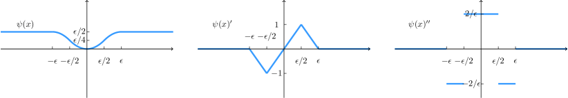
Figure 2: $\psi(x)$, $\psi(x)^{\prime}$ and $\psi(x)^{\prime\prime}$. For $\epsilon_{\mathrm{mp}}\in(0,1)$.

Lemma 5.10 (Properties of function $\psi$).

Let function $\psi$ be defined in (21). Then function $\psi$ satisfies the following properties:
1. Symmetric $(\psi(-x)=\psi(x))$ and $\psi(0)=0$;
2. $\psi(|x|)$ is non-decreasing;
3. $|\psi^{\prime}(x)|=\Omega(1),\forall|x|\in[0.01\epsilon_{\mathrm{mp}},\epsilon_{\mathrm{mp}}]$;
4. $L_{1}\stackrel{{\scriptstyle\mathrm{{\scriptscriptstyle def}}}}{{=}}\max_{x}\psi^{\prime}(x)=1$ and $L_{2}\stackrel{{\scriptstyle\mathrm{{\scriptscriptstyle def}}}}{{=}}\max_{x}\psi^{\prime\prime}(x)=1/\epsilon_{\mathrm{mp}}$.

Proof.

We can see that

$$\psi(x)^{\prime}=\begin{cases}\frac{2|x|}{\epsilon_{\mathrm{mp}}},&|x|\in[0,\epsilon_{\mathrm{mp}}/2]\\ \frac{2(\epsilon_{\mathrm{mp}}-|x|)}{\epsilon_{\mathrm{mp}}},&|x|\in(\epsilon_{\mathrm{mp}}/2,\epsilon_{\mathrm{mp}}]\\ 0,&|x|\in(\epsilon_{\mathrm{mp}},+\infty)\end{cases}\quad\text{and}\quad\psi(x)^{\prime\prime}=\begin{cases}\frac{2}{\epsilon_{\mathrm{mp}}},&x\in[0,\epsilon_{\mathrm{mp}}/2]\cup[-\epsilon_{\mathrm{mp}},-\epsilon_{\mathrm{mp}}/2]\\ -\frac{2}{\epsilon_{\mathrm{mp}}},&x\in(\epsilon_{\mathrm{mp}}/2,\epsilon_{\mathrm{mp}}]\cup[-\epsilon_{\mathrm{mp}}/2,0]\\ 0.&|x|\in(\epsilon_{\mathrm{mp}},+\infty)\end{cases}$$

From the $\psi(x)^{\prime}$ and $\psi(x)^{\prime\prime}$, it is not hard to see that $\psi$ satisfies the properties needed. ∎

Acknowledgement

This work was supported in part by NSF Awards CCF-1740551, CCF-1749609, and DMS-1839116. We thank Sébastien Bubeck and Aaron Sidford for helpful discussions. We thank Rasmus Kyng for bringing up the question and providing some fixes in the proof of projection maintenance. We thank Josh Alman for some useful discussions about matrix multiplication. We thank Swati Padmanabhan for writing suggestions. We thank Eric Price for the suggestion of the title of this paper. We thank Shunhua Jiang and Hengjie Zhang for drawing several beautiful pictures. Finally, we thank anonymous STOC and JACM reviewers for their detailed feedback.

Appendix A Appendix

Lemma A.1.

Let $x$ and $y$ denote (possibly dependent) random variables such that $|x|\leq c_{x}$ and $|y|\leq c_{y}$ almost surely. Then, we have

$$\operatorname*{{\bf{Var}}}[xy]\leq 2c_{x}^{2}\cdot\operatorname*{{\bf{Var}}}[y]+2c_{y}^{2}\cdot\operatorname*{{\bf{Var}}}[x].$$

Proof.

Recall that $\operatorname*{{\bf{Var}}}[xy]\leq\operatorname*{{\bf{E}}}[(xy-t)^{2}]$ for any scalar $t$. Hence,

$$\operatorname*{{\bf{Var}}}[xy] \leq\operatorname*{{\bf{E}}}[(xy-\operatorname*{{\bf{E}}}[x]\operatorname*{{\bf{E}}}[y])^{2}]=\operatorname*{{\bf{E}}}[(xy-x\operatorname*{{\bf{E}}}[y]+x\operatorname*{{\bf{E}}}[y]-\operatorname*{{\bf{E}}}[x]\operatorname*{{\bf{E}}}[y])^{2}]$$

$$\leq 2\operatorname*{{\bf{E}}}[(xy-x\operatorname*{{\bf{E}}}[y])^{2}]+2\operatorname*{{\bf{E}}}[(x\operatorname*{{\bf{E}}}[y]-\operatorname*{{\bf{E}}}[x]\operatorname*{{\bf{E}}}[y])^{2}]$$

$$\leq 2c_{x}^{2}\cdot\operatorname*{{\bf{Var}}}[y]+2c_{y}^{2}\cdot\operatorname*{{\bf{Var}}}[x].$$

∎

Lemma A.2 ([Vai89b]).

Given a matrix $A\in\mathbb{R}^{d\times n}$, vectors $b\in\mathbb{R}^{d},c\in\mathbb{R}^{n}$. Suppose $x,s,y\in\mathbb{R}^{n}$ satisfy that $xs\approx_{0.1}t$, $Ax=b$ and $A^{\top}y+s=c$ for some $t>0$. For any $\epsilon\in(0,1/2]$, in $\widetilde{O}(n^{2.5}\log(n/\epsilon))$ time, we can find vectors $x^{\operatorname{new}},s^{\operatorname{new}}\in\mathbb{R}^{n}$ and $y^{\operatorname{new}}\in\mathbb{R}^{d}$ such that

$$\|x^{\operatorname{new}}s^{\operatorname{new}}-t\|_{2}\leq \leavevmode\nobreak\ \epsilon,$$

$$Ax^{\operatorname{new}}= \leavevmode\nobreak\ b,$$

$$A^{\top}y^{\operatorname{new}}+s= \leavevmode\nobreak\ c.$$

Remark A.3.

Instead of using the algorithm in [Vai89b], one can also run our algorithm with $k=n$ for $O(\sqrt{n}\log n)$ iterations. Since $k=n$, there is no randomness involved and hence $\Phi$ will decrease deterministically to $O(n)$.

Lemma A.4.

$\omega\leq 3-\alpha$.

Proof.

We consider a $n\times n$ matrix $A$ multiply another $n\times n$ matrix $B$. We split $A$ into $n^{1-\alpha}$ fat matrices where each of them has size $n^{\alpha}\times n$. Since $\omega$ is the best exponent of matrix multiplication, thus we know

$$n^{\omega+o(1)}\leq n^{1-\alpha}\cdot n^{2+o(1)}.$$

Taking $n\rightarrow\infty$, this implies $\omega\leq 3-\alpha$. ∎

Note that the bound in Lemma A.4 can be improved to $\omega+\frac{1}{2}\omega\alpha\leq 3$ [CGLZ20] via tensor rank.

Lemma A.5 (Rectangular matrix multiplication).

For any $n\geq r$, multiplying an $n\times r$ with an $r\times n$ matrix or $n\times n$ with $n\times r$ takes time

$$n^{2+o(1)}+r^{\frac{\omega-2}{1-\alpha}}n^{2-\frac{\alpha(\omega-2)}{1-\alpha}+o(1)}.$$

Proof.

The cost for multiplying a $n\times n$ and a $n\times r$ matrix is the same as multiplying a $n\times r$ and a $r\times n$ matrix [Pan84, page 51]. So, we focus on the later case.

For the case $r\leq n^{\alpha}$, it follows from the rectangular matrix multiplication result in [LGU18].

For the case $r\geq n^{\alpha}$, we let $k=(n/r)^{\frac{1}{1-\alpha}}$. We can view the problem as multiplying a $k\times k^{\alpha}$ and a $k^{\alpha}\times k$ block matrices and each block has size $\frac{n}{k}\times\frac{n}{k}$ size. Therefore, the total cost is

$$k^{2+o(1)}\times(\frac{n}{k})^{\omega+o(1)}=r^{\frac{\omega-2}{1-\alpha}}n^{2-\frac{\alpha(\omega-2)}{1-\alpha}+o(1)}.$$

∎

Lemma A.6.

Let $A\in\mathbb{R}^{d\times n}$, $b\in\mathbb{R}^{d}$ and $c\in\mathbb{R}^{n}$. For a matrix $A$, we define $\|A\|_{1}$ to be $\sum_{i,j}|A_{i,j}|$. Given a linear program $\min_{Ax=b,x\geq 0}c^{\top}x$ with $n$ variables and $d$ constraints. Assume that
1. Diameter of the polytope : For any $x\geq 0$ with $Ax=b$, we have that $\|x\|_{\infty}\leq R$.
2. Lipschitz constant of the linear program : $\|c\|_{\infty}\leq L$.

For any $\delta\in(0,1]$, the modified linear program $\min_{\overline{A}\overline{x}=\overline{b},\overline{x}\geq 0}\overline{c}^{\top}\overline{x}$ with

$$\overline{A}=\begin{bmatrix}A&0&\frac{1}{R}b-A1_{n}\\ 1_{n}^{\top}&1&0\end{bmatrix}\in\mathbb{R}^{(d+1)\times(n+2)},\overline{b}=\begin{bmatrix}\frac{1}{R}b\\ n+1\end{bmatrix}\in\mathbb{R}^{d+1}\text{\leavevmode\nobreak\ and,\leavevmode\nobreak\ }\overline{c}=\begin{bmatrix}\frac{\delta}{L}\cdot c\\ 0\\ 1\end{bmatrix}\in\mathbb{R}^{n+2}$$

satisfies the following :
1. $\overline{x}=\begin{bmatrix}1_{n}\\ 1\\ 1\end{bmatrix}\in\mathbb{R}^{n+2}$, $\overline{y}=\begin{bmatrix}0_{d}\\ -1\end{bmatrix}\in\mathbb{R}^{d+1}$ and $\overline{s}=\begin{bmatrix}1_{n}+\frac{\delta}{L}\cdot c\\ 1\\ 1\end{bmatrix}\in\mathbb{R}^{n+2}$ are feasible primal dual vectors.
2. For any feasible primal dual vectors $(\overline{x},\overline{y},\overline{s})\in\mathbb{R}^{(n+2)\times(d+1)\times(n+2)}$ with duality gap $\leq\delta^{2}$, the vector $\widehat{x}=R\cdot\overline{x}_{1:n}\in\mathbb{R}^{n}$ ($\overline{x}_{1:n}$ is the first $n$ coordinates of $x$) is an approximate solution to the original linear program in the following sense

$$c^{\top}\widehat{x}\leq \leavevmode\nobreak\ \min_{Ax=b,x\geq 0}c^{\top}x+LR\cdot\delta,$$

$$\|A\widehat{x}-b\|_{1}\leq \leavevmode\nobreak\ 4n\delta\cdot(R\|A\|_{1}+\|b\|_{1}),$$

$$\widehat{x}\geq \leavevmode\nobreak\ 0.$$

Proof.

Part 1. For the first result, straightforward calculations show that $(\overline{x},\overline{y},\overline{s})\in\mathbb{R}^{(n+2)\times(d+1)\times(n+2)}$ are feasible, i.e.,

$$\overline{A}\overline{x}=\begin{bmatrix}A&0&\frac{1}{R}b-A1_{n}\\ 1_{n}^{\top}&1&0\end{bmatrix}\cdot\begin{bmatrix}1_{n}\\ 1\\ 1\end{bmatrix}=\begin{bmatrix}\frac{1}{R}b\\ n+1\end{bmatrix}=\overline{b}$$

and

$$\overline{A}^{\top}\overline{y}+\overline{s}= \leavevmode\nobreak\ \begin{bmatrix}A^{\top}&1_{n}\\ 0&1\\ \frac{1}{R}b^{\top}-1_{n}^{\top}A^{\top}&0\\ \end{bmatrix}\cdot\begin{bmatrix}0_{d}\\ -1\end{bmatrix}+\begin{bmatrix}1_{n}+\frac{\delta}{L}\cdot c\\ 1\\ 1\end{bmatrix}$$

$$= \leavevmode\nobreak\ \begin{bmatrix}-1_{n}\\ -1\\ 0\\ \end{bmatrix}+\begin{bmatrix}1_{n}+\frac{\delta}{L}\cdot c\\ 1\\ 1\end{bmatrix}$$

$$= \leavevmode\nobreak\ \begin{bmatrix}\frac{\delta}{L}\cdot c\\ 0\\ 1\end{bmatrix}$$

$$= \leavevmode\nobreak\ \overline{c}$$

Part 2. For the second result, we let

$$\operatorname{OPT}=\min_{Ax=b,x\geq 0}c^{\top}x,\text{\leavevmode\nobreak\ \leavevmode\nobreak\ \leavevmode\nobreak\ and,\leavevmode\nobreak\ \leavevmode\nobreak\ \leavevmode\nobreak\ }\overline{\operatorname{OPT}}=\min_{\overline{A}\overline{x}=\overline{b},\overline{x}\geq 0}\overline{c}^{\top}\overline{x}.$$

For any optimal $x\in\mathbb{R}^{n}$ in the original LP, we consider the following $\overline{x}\in\mathbb{R}^{n+2}$

$$\overline{x}=\begin{bmatrix}\frac{1}{R}x\\ n+1-\frac{1}{R}\sum_{i=1}^{n}x_{i}\\ 0\end{bmatrix}$$ (25)

and $\overline{c}\in\mathbb{R}^{n+2}$

$$\overline{c}=\begin{bmatrix}\frac{\delta}{L}\cdot c^{\top}\\ 0\\ 1\end{bmatrix}$$ (26)

We want to argue that $\overline{x}\in\mathbb{R}^{n+2}$ is feasible in the modified LP. It is obvious that $\overline{x}\geq 0$, it remains to show $\overline{A}\overline{x}=\overline{b}\in\mathbb{R}^{d+1}$. We have

$$\overline{A}\overline{x}=\begin{bmatrix}A&0&\frac{1}{R}b-A1_{n}\\ 1_{n}^{\top}&1&0\end{bmatrix}\cdot\begin{bmatrix}\frac{1}{R}x\\ n+1-\frac{1}{R}\sum_{i=1}^{n}x_{i}\\ 0\end{bmatrix}=\begin{bmatrix}\frac{1}{R}Ax\\ n+1\end{bmatrix}=\begin{bmatrix}\frac{1}{R}b\\ n+1\end{bmatrix}=\overline{b},$$

where the third step follows from $Ax=b$, and the last step follows from the definition of $\overline{b}$.

Therefore, using the definition of $\overline{x}$ in (25) we have that

$$\overline{\operatorname{OPT}}\leq\overline{c}^{\top}\overline{x}=\begin{bmatrix}\frac{\delta}{L}\cdot c^{\top}&0&1\end{bmatrix}\cdot\begin{bmatrix}\frac{1}{R}x\\ n+1-\frac{1}{R}\sum_{i=1}^{n}x_{i}\\ 0\end{bmatrix}=\frac{\delta}{LR}\cdot c^{\top}x=\frac{\delta}{LR}\cdot\operatorname{OPT}.$$ (27)

where the first step follows from the fact that modified program is a minimization problem, the second step follows from the definitions of $\overline{x}\in\mathbb{R}^{n+2}$ (25) and $\overline{c}\in\mathbb{R}^{n+2}$ (26), the last step follows from the fact that $x\in\mathbb{R}^{n}$ is an optimal solution in the original linear program.

Given a feasible $(\overline{x},\overline{y},\overline{s})\in\mathbb{R}^{(n+2)\times(d+1)\times(n+2)}$ with duality gap $\delta^{2}$. Write $\overline{x}=\begin{bmatrix}\overline{x}_{1:n}\\ \tau\\ \theta\end{bmatrix}\in\mathbb{R}^{n+2}$ for some $\tau\geq 0$, $\theta\geq 0$. We can compute $\overline{c}^{\top}\overline{x}$ which is $\frac{\delta}{L}\cdot c^{\top}\overline{x}_{1:n}+\theta$. Then, we have

$$\frac{\delta}{L}\cdot c^{\top}\overline{x}_{1:n}+\theta\leq\overline{\operatorname{OPT}}+\delta^{2}\leq\frac{\delta}{LR}\cdot\operatorname{OPT}+\delta^{2},$$ (28)

where the first step follows from definition of duality gap, the last step follows from (27).

Hence, we can upper bound the $\operatorname{OPT}$ of the transformed program as follows:

$$c^{\top}\widehat{x}=R\cdot c^{\top}\overline{x}_{1:n}=\frac{LR}{\delta}\cdot\frac{\delta}{L}c^{\top}\overline{x}_{1:n}\leq\frac{RL}{\delta}(\frac{\delta}{LR}\cdot\operatorname{OPT}+\delta^{2})=\operatorname{OPT}+LR\cdot\delta,$$

where the first step follows by $\widehat{x}=R\cdot\overline{x}_{1:n}$, the third step follows by (28).

Note that

$$\frac{\delta}{L}c^{\top}\overline{x}_{1:n}\geq-\frac{\delta}{L}\|c\|_{\infty}\|\overline{x}_{1:n}\|_{1}=-\frac{\delta}{L}\|c\|_{\infty}\|\frac{1}{R}x\|_{1}\geq-\frac{\delta}{L}\|c\|_{\infty}\frac{n}{R}\|x\|_{\infty}\geq-\delta n,$$ (29)

where the second step follows from the definition of $\overline{x}\in\mathbb{R}^{n+2}$, and the last step follows from $\|c\|_{\infty}\leq L$ and $\|x\|_{\infty}\leq R$.

We can upper bound the $\theta$ in the following sense,

$$\theta\leq\frac{\delta}{LR}\cdot\operatorname{OPT}+\delta^{2}+\delta n\leq 2n\delta+\delta^{2}\leq 4n\delta$$ (30)

where the first step follows from (28) and (29), the second step follows by $\operatorname{OPT}=\min_{Ax=b,x\geq 0}c^{\top}x\leq nLR$ (because $\|c\|_{\infty}\leq L$ and $\|x\|_{\infty}\leq R$), and the last step follows from $\delta\leq 1\leq n$.

The constraint in the new polytope shows that

$$A\overline{x}_{1:n}+(\frac{1}{R}b-A1_{n})\theta=\frac{1}{R}b.$$

Using $\widehat{x}=Rx_{1:n}\in\mathbb{R}^{n}$, we have

$$A\frac{1}{R}\widehat{x}+(\frac{1}{R}b-A1_{n})\theta=\frac{1}{R}b.$$

Rewriting it, we have $A\widehat{x}-b=(RA1_{n}-b)\theta\in\mathbb{R}^{d}$ and hence

$$\|A\widehat{x}-b\|_{1}=\|(RA1_{n}-b)\theta\|_{1}\leq\theta(\|RA1_{n}\|_{1}+\|b\|_{1})\leq\theta\cdot(R\|A\|_{1}+\|b\|_{1})\leq 4n\delta\cdot(R\|A\|_{1}+\|b\|_{1}),$$

where the second step follows from the triangle inequality, the third step follows from $\|A1_{n}\|_{1}\leq\|A\|_{1}$ (because the definition of entry-wise $\ell_{1}$ norm), and the last step follows from (30).

Thus, we complete the proof. ∎

Appendix B Generalized Projection Maintenance

Given the usefulness of projection maintenance, we state a more general version of Theorem 5.1 for future use.

Theorem B.1.

Assume the following about the cost of matrix operations:

• In $O(t_{k})$ time, we can multiply a $n\times n$ and a $n\times k$ matrix, and we can multiply a $n\times k$ and a $k\times n$ matrix.

• In $O(s_{n})$ time, we can invert a $n\times n$ matrix, and we can multiply a $n\times n$ and a $n\times n$ matrix.

• $t_{k}/k$ is decreasing $k$.

Given a matrix $A\in\mathbb{R}^{d\times n}$ with $n\geq d$, a tolerance parameter $0<\epsilon_{\mathrm{mp}}<1/4$ and $k^{*}\in[n]$, there is a deterministic data structure that approximately maintains the projection matrices

$$\sqrt{W}A^{\top}(AWA^{\top})^{-1}A\sqrt{W}$$

and the inverse matrices $(AWA^{\top})^{-1}\in\mathbb{R}^{d\times d}$ for positive diagonal matrices $W\in\mathbb{R}^{n\times n}$ through the following operations:

• $\textsc{Update}(w)$: Output a vector $\widetilde{v}$ such that for all $i$,

  $$(1-\epsilon_{\mathrm{mp}})\widetilde{v_{i}}\leq w_{i}\leq(1+\epsilon_{\mathrm{mp}})\widetilde{v_{i}}.$$

• $\textsc{Query}_{1}(h)$: Output $\sqrt{\widetilde{V}}A^{\top}(A\widetilde{V}A^{\top})^{-1}A\sqrt{\widetilde{V}}h\in\mathbb{R}^{n}$ for the $\widetilde{v}$ outputted by the last call to Update.

• $\textsc{Query}_{2}(h)$: Output $(A\widetilde{V}A^{\top})^{-1}h\in\mathbb{R}^{d}$ for the $\widetilde{v}$ outputted by the last call to Update.

• $\textsc{Insert}(a,w_{a})$: Insert a column $a$ into $A$, a weight $w_{a}$ into $w$.

• $\textsc{Delete}(a)$: Delete a column $a$ from $A$ and its corresponding weight from $w$.

• $\textsc{Output}()$: Output $\sqrt{\widetilde{V}}A^{\top}(A\widetilde{V}A^{\top})^{-1}A\sqrt{\widetilde{V}}\in\mathbb{R}^{n\times n}$ and $(A\widetilde{V}A^{\top})^{-1}\in\mathbb{R}^{d\times d}$ for the $\widetilde{v}$ outputted by the last call to Update.

Suppose that the number of columns is $O(n)$ during the whole algorithm and that for any call of Update, we have

$$\sum_{i=1}^{n}\left(\operatorname*{{\bf{E}}}[\ln w_{i}]-\ln(w_{i}^{\mathrm{old}})\right)^{2}\leq C_{1}^{2}\qquad\text{and}\qquad\sum_{i=1}^{n}(\operatorname*{{\bf{Var}}}[\ln(w_{i})])^{2}\leq C_{2}^{2}$$

where $w$ is the input of call, $w^{\mathrm{old}}$ is the weight before the call, and the expectation and variance is conditional on $w_{i}^{\mathrm{old}}$. Then, we have that:

• The data structure takes $O(s_{n}+t_{n})$ time to initialize.

• Each call of Query takes time $O(n\cdot\|h\|_{0}+s_{k^{*}}+nk^{*})$.

• Each call of $\textsc{Output}()$ takes $O(t_{k^{*}})$ time.

• Each call of Insert and Delete takes $O(n^{2})$ time.

• Each call of Update takes

  $$O\left((C_{1}/\epsilon_{\mathrm{mp}}+C_{2}/\epsilon_{\mathrm{mp}}^{2})\cdot\left(\frac{t_{k^{*}}^{2}}{k^{*}}+\sum_{i=k^{*}}^{n}\frac{t_{i}^{2}}{i^{2}}\right)^{1/2}\cdot\log n\right)$$

  expected time in amortized.

Proof.

The proof is essentially the same as Theorem 5.1. The way to maintain $A\widetilde{V}A^{\top}\in\mathbb{R}^{d\times d}$ is almost identical to $\sqrt{\widetilde{V}}A^{\top}(A\widetilde{V}A^{\top})^{-1}A\sqrt{\widetilde{V}}h\in\mathbb{R}^{n}$. Updating both matrices under insertion and deletion can be done via Sherman Morrison formula in $O(n^{2})$ time. We note that these updates does not increase our potential and hence it does not affect the amortized cost for Update. Finally, to bound the runtime using $t_{k}$ and $s_{n}$ instead of $\alpha$ and $\omega$, we use the same potential $\Psi_{k}=\sum_{i=1}^{n}g_{i}\psi(x_{i}^{(k)})$ with a new definition of $g$:

$$g_{i}=\begin{cases}t_{i}/i,&\text{if }i\geq k^{*};\\ t_{k^{*}}/k^{*},&\text{otherwise}.\end{cases}.$$

Now, the update time in Lemma 5.4 becomes $O(rg_{r})$. The rest of the proof is identical. In particular, Lemma 5.8 becomes

$$\|g\|_{2}=\left(\frac{t_{k^{*}}}{k^{*}}+\sum_{i=k^{*}}^{n}\frac{t_{i}^{2}}{i^{2}}\right)^{1/2}$$

and hence Lemma 5.7 gives the bound

$$O(C_{1}+C_{2}/\epsilon_{\mathrm{mp}})\cdot\left(\frac{t_{k^{*}}}{k^{*}}+\sum_{i=k^{*}}^{n}\frac{t_{i}^{2}}{i^{2}}\right)^{1/2}.$$

∎

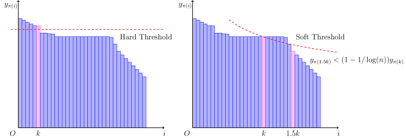
Figure 3: In this figure we illustrate the naive hard threshold and the soft threshold. The x-axis represents the sorted $n$ coordinates, and the y-axis represents the errors $y_{\pi(i)}$. All the coordinates smaller than the threshold $k$ are updated. In the left figure, we choose the hard threshold $k$ as the smallest coordinates such that $y_{\pi(k)}\leq\epsilon_{\mathrm{mp}}$. In the right figure, we choose the soft threshold $k$ as the smallest coordinates that satisfies both $y_{\pi(k)}\leq\epsilon_{\mathrm{mp}}$ and $y_{\pi(1.5k)}<(1-1/\log(n))y_{\pi(k)}$.

References

- [AFLG15] Andris Ambainis, Yuval Filmus, and François Le Gall. Fast matrix multiplication: limitations of the coppersmith-winograd method. In Proceedings of the forty-seventh annual ACM symposium on Theory of computing (STOC), pages 585–593. ACM, 2015.
- [Alm19] Josh Alman. Limits on the universal method for matrix multiplication. In 34th Computational Complexity Conference (CCC), pages 12:1–12:24, 2019.
- [AW18] Josh Alman and Virginia Vassilevska Williams. Limits on all known (and some unknown) approaches to matrix multiplication. In 2018 IEEE 59th Annual Symposium on Foundations of Computer Science (FOCS). IEEE, 2018.
- [BCLL18] Sébastien Bubeck, Michael B Cohen, Yin Tat Lee, and Yuanzhi Li. An homotopy method for regression provably beyond self-concordance and in input-sparsity time. In Proceedings of the 50th Annual ACM SIGACT Symposium on Theory of Computing (STOC), pages 1130–1137. ACM, 2018.
- [BLSS20] Jan van den Brand, Yin Tat Lee, Aaron Sidford, and Zhao Song. Solving tall dense linear programs in nearly linear time. In 52nd Annual ACM Symposium on Theory of Computing (STOC), pages 775–788, 2020.
- [BPSW20] Jan van den Brand, Binghui Peng, Zhao Song, and Omri Weinstein. Training (overparametrized) neural networks in near-linear time. arXiv preprint arXiv:2006.11648, 2020.
- [Bra20] Jan van den Brand. A deterministic linear program solver in current matrix multiplication time. In Proceedings of the Fourteenth Annual ACM-SIAM Symposium on Discrete Algorithms (SODA), pages 259–278. SIAM, 2020.
- [CGLZ20] Matthias Christandl, François Le Gall, Vladimir Lysikov, and Jeroen Zuiddam. Barriers for rectangular matrix multiplication. In 35th Computational Complexity Conference (CCC). https://arXiv.org/pdf/2003.03019.pdf, 2020.
- [CKK+18] Michael B Cohen, Jonathan Kelner, Rasmus Kyng, John Peebles, Richard Peng, Anup B Rao, and Aaron Sidford. Solving directed laplacian systems in nearly-linear time through sparse LU factorizations. In 2018 IEEE 59th Annual Symposium on Foundations of Computer Science (FOCS), pages 898–909. IEEE, 2018.
- [CKL18] Diptarka Chakraborty, Lior Kamma, and Kasper Green Larsen. Tight cell probe bounds for succinct boolean matrix-vector multiplication. In Proceedings of the 50th Annual ACM SIGACT Symposium on Theory of Computing (STOC), pages 1297–1306, 2018.
- [CKM+11] Paul Christiano, Jonathan A Kelner, Aleksander Madry, Daniel A Spielman, and Shang-Hua Teng. Electrical flows, laplacian systems, and faster approximation of maximum flow in undirected graphs. In Proceedings of the forty-third annual ACM symposium on Theory of computing (STOC), pages 273–282. ACM, 2011.
- [CKM+14] Michael B Cohen, Rasmus Kyng, Gary L Miller, Jakub W Pachocki, Richard Peng, Anup B Rao, and Shen Chen Xu. Solving sdd linear systems in nearly time. In Proceedings of the forty-sixth annual ACM symposium on Theory of computing (STOC), pages 343–352. ACM, 2014.
- [CLM+16] Michael B Cohen, Yin Tat Lee, Gary Miller, Jakub Pachocki, and Aaron Sidford. Geometric median in nearly linear time. In Proceedings of the forty-eighth annual ACM symposium on Theory of Computing (STOC), pages 9–21. ACM, 2016.
- [CLP+20] Beidi Chen, Zichang Liu, Binghui Peng, Zhaozhuo Xu, Jonathan Lingjie Li, Tri Dao, Zhao Song, Anshumali Shrivastava, and Christopher Re. Mongoose: A learnable lsh framework for efficient neural network training. In OpenReview.net. https://openreview.net/forum?id=wWK7yXkULyh, 2020.
- [CMSV17] Michael B Cohen, Aleksander Mądry, Piotr Sankowski, and Adrian Vladu. Negative-weight shortest paths and unit capacity minimum cost flow in time. In Proceedings of the Twenty-Eighth Annual ACM-SIAM Symposium on Discrete Algorithms (SODA), pages 752–771. SIAM, 2017.
- [CMTV17] Michael B Cohen, Aleksander Madry, Dimitris Tsipras, and Adrian Vladu. Matrix scaling and balancing via box constrained newton’s method and interior point methods. In 58th Annual Symposium on Foundations of Computer Science (FOCS), pages 902–913. IEEE, 2017.
- [CW87] Don Coppersmith and Shmuel Winograd. Matrix multiplication via arithmetic progressions. In Proceedings of the nineteenth annual ACM symposium on Theory of computing (STOC), pages 1–6. ACM, 1987.
- [CW13] Kenneth L. Clarkson and David P. Woodruff. Low rank approximation and regression in input sparsity time. In Symposium on Theory of Computing Conference (STOC), pages 81–90. https://arxiv.org/pdf/1207.6365, 2013.
- [DS13] Alexander Munro Davie and Andrew James Stothers. Improved bound for complexity of matrix multiplication. Proceedings of the Royal Society of Edinburgh Section A: Mathematics, 143(2):351–369, 2013.
- [HKNS15] Monika Henzinger, Sebastian Krinninger, Danupon Nanongkai, and Thatchaphol Saranurak. Unifying and strengthening hardness for dynamic problems via the online matrix-vector multiplication conjecture. In Proceedings of the forty-seventh annual ACM symposium on Theory of computing (STOC), pages 21–30, 2015.
- [JKL+20] Haotian Jiang, Tarun Kathuria, Yin Tat Lee, Swati Padmanabhan, and Zhao Song. A faster interior point method for semidefinite programming. In 61st Annual IEEE Symposium on Foundations of Computer Science (FOCS). https://arxiv.org/pdf/2009.10217.pdf, 2020.
- [JLSW20] Haotian Jiang, Yin Tat Lee, Zhao Song, and Sam Chiu-wai Wong. An improved cutting plane method for convex optimization, convex-concave games and its applications. In 52nd Annual ACM Symposium on Theory of Computing (STOC), pages 944–953. https://arxiv.org/pdf/2004.04250.pdf, 2020.
- [JSWZ20] Shunhua Jiang, Zhao Song, Omri Weinstein, and Hengjie Zhang. Faster dynamic matrix inverse for faster lps. In arXiv preprint. https://arxiv.org/2004.07470, 2020.
- [Kar84] Narendra Karmarkar. A new polynomial-time algorithm for linear programming. In Proceedings of the sixteenth annual ACM symposium on Theory of computing (STOC), pages 302–311. ACM, 1984.
- [KLP+16] Rasmus Kyng, Yin Tat Lee, Richard Peng, Sushant Sachdeva, and Daniel A Spielman. Sparsified cholesky and multigrid solvers for connection laplacians. In Proceedings of the forty-eighth annual ACM symposium on Theory of Computing (STOC), pages 842–850. ACM, 2016.
- [KMP10] Ioannis Koutis, Gary L Miller, and Richard Peng. Approaching optimality for solving sdd linear systems. In 2010 IEEE 51st Annual Symposium on Foundations of Computer Science (FOCS), pages 235–244. IEEE, 2010.
- [KMP11] Ioannis Koutis, Gary L Miller, and Richard Peng. A nearly-m log n time solver for sdd linear systems. In 2011 IEEE 52nd Annual Symposium on Foundations of Computer Science (FOCS), pages 590–598. IEEE, 2011.
- [KOSZ13] Jonathan A Kelner, Lorenzo Orecchia, Aaron Sidford, and Zeyuan Allen Zhu. A simple, combinatorial algorithm for solving sdd systems in nearly-linear time. In Proceedings of the forty-fifth annual ACM symposium on Theory of computing (STOC), pages 911–920. ACM, https://arxiv.org/pdf/1301.6628.pdf, 2013.
- [KPSZ18] Rasmus Kyng, Richard Peng, Robert Schwieterman, and Peng Zhang. Incomplete nested dissection. In Proceedings of the 50th Annual ACM SIGACT Symposium on Theory of Computing (STOC), pages 404–417. ACM, 2018.
- [KS16] Rasmus Kyng and Sushant Sachdeva. Approximate gaussian elimination for laplacians-fast, sparse, and simple. In 2016 IEEE 57th Annual Symposium on Foundations of Computer Science (FOCS), pages 573–582. IEEE, 2016.
- [LG14] François Le Gall. Powers of tensors and fast matrix multiplication. In Proceedings of the 39th international symposium on symbolic and algebraic computation (ISSAC), pages 296–303. ACM, https://arxiv.org/pdf/1401.7714.pdf, 2014.
- [LGU18] Francois Le Gall and Florent Urrutia. Improved rectangular matrix multiplication using powers of the coppersmith-winograd tensor. In Proceedings of the Twenty-Ninth Annual ACM-SIAM Symposium on Discrete Algorithms (SODA), pages 1029–1046. SIAM, 2018.
- [LS13] Yin Tat Lee and Aaron Sidford. Path finding I: Solving linear programs with linear system solves. arXiv preprint arXiv:1312.6677, 2013.
- [LS14] Yin Tat Lee and Aaron Sidford. Path finding methods for linear programming: Solving linear programs in iterations and faster algorithms for maximum flow. In 2014 IEEE 55th Annual Symposium on Foundations of Computer Science (FOCS), pages 424–433. IEEE, 2014.
- [LS15] Yin Tat Lee and Aaron Sidford. Efficient inverse maintenance and faster algorithms for linear programming. In 56th Annual Symposium on Foundations of Computer Science (FOCS), pages 230–249. IEEE, 2015.
- [LSW15] Yin Tat Lee, Aaron Sidford, and Sam Chiu-wai Wong. A faster cutting plane method and its implications for combinatorial and convex optimization. In 56th Annual Symposium on Foundations of Computer Science (FOCS), pages 1049–1065. IEEE, 2015.
- [LSZ19] Yin Tat Lee, Zhao Song, and Qiuyi Zhang. Solving empirical risk minimization in the current matrix multiplication time. In Conference on Learning Theory (COLT), pages 2140–2157. https://arxiv.org/pdf/1905.04447.pdf, 2019.
- [LSZ20] S Cliff Liu, Zhao Song, and Hengjie Zhang. Breaking the -pass barrier: A streaming algorithm for maximum weight bipartite matching. arXiv preprint arXiv:2009.06106, 2020.
- [LW17] Kasper Green Larsen and Ryan Williams. Faster online matrix-vector multiplication. In Proceedings of the Twenty-Eighth Annual ACM-SIAM Symposium on Discrete Algorithms (SODA), pages 2182–2189. SIAM, 2017.
- [Mad13] Aleksander Madry. Navigating central path with electrical flows: From flows to matchings, and back. In 2013 IEEE 54th Annual Symposium on Foundations of Computer Science (FOCS), pages 253–262. IEEE, 2013.
- [Mad16] Aleksander Madry. Computing maximum flow with augmenting electrical flows. In 2016 IEEE 57th Annual Symposium on Foundations of Computer Science (FOCS), pages 593–602. IEEE, 2016.
- [Meg12] Nimrod Megiddo. Progress in Mathematical Programming: Interior-Point and Related Methods. Springer Science & Business Media, 2012.
- [NN89] Yu Nesterov and Arkadi Nemirovsky. Self-concordant functions and polynomial-time methods in convex programming. Report, Central Economic and Mathematic Institute, USSR Acad. Sci, 1989.
- [NN91] Yu Nesterov and Arkadi Nemirovsky. Acceleration and parallelization of the path-following interior point method for a linearly constrained convex quadratic problem. SIAM Journal on Optimization, 1(4):548–564, 1991.
- [NN94] Yurii Nesterov and Arkadii Nemirovskii. Interior-point polynomial algorithms in convex programming, volume 13. Siam, 1994.
- [NN13] Jelani Nelson and Huy L Nguyên. Osnap: Faster numerical linear algebra algorithms via sparser subspace embeddings. In 2013 IEEE 54th Annual Symposium on Foundations of Computer Science (FOCS), pages 117–126. IEEE, https://arxiv.org/pdf/1211.1002, 2013.
- [Pan84] Victor Pan. How to multiply matrices faster. Lecture notes in computer science, 179, 1984.
- [PRT02] Jiming Peng, Cornelis Roos, and Tamás Terlaky. Self-regular functions and new search directions for linear and semidefinite optimization. Mathematical Programming, 93(1):129–171, 2002.
- [Ren88] James Renegar. A polynomial-time algorithm, based on newton’s method, for linear programming. Mathematical Programming, 40(1-3):59–93, 1988.
- [Ren01] James Renegar. A mathematical view of interior-point methods in convex optimization, volume 3. Siam, 2001.
- [RTV05] Cornelis Roos, Tamás Terlaky, and J-Ph Vial. Interior point methods for linear optimization. Springer Science & Business Media, 2005.
- [Sar06] Tamás Sarlós. Improved approximation algorithms for large matrices via random projections. In 47th Annual Symposium on Foundations of Computer Science (FOCS), pages 143–152. IEEE, 2006.
- [SS11] Daniel A Spielman and Nikhil Srivastava. Graph sparsification by effective resistances. SIAM Journal on Computing, 40(6):1913–1926, 2011.
- [ST04] Daniel A. Spielman and Shang-Hua Teng. Nearly-linear time algorithms for graph partitioning, graph sparsification, and solving linear systems. In Proceedings of the Thirty-sixth Annual ACM Symposium on Theory of Computing (STOC), pages 81–90. ACM, 2004.
- [SY20] Zhao Song and Zheng Yu. Oblivious sketching-based central path method for solving linear programming problems. In OpenReview.net. https://openreview.net/forum?id=fGiKxvF-eub, 2020.
- [Ter13] Tamás Terlaky. Interior point methods of mathematical programming, volume 5. Springer Science & Business Media, 2013.
- [Vai87] Pravin M Vaidya. An algorithm for linear programming which requires arithmetic operations. In In Proceedings of the nineteenth annual ACM symposium on Theory of computing (STOC), pages 29–38. ACM, 1987.
- [Vai89a] Pravin M Vaidya. A new algorithm for minimizing convex functions over convex sets. In 30th Annual Symposium on Foundations of Computer Science (FOCS), pages 338–343. IEEE, 1989.
- [Vai89b] Pravin M Vaidya. Speeding-up linear programming using fast matrix multiplication. In 30th Annual Symposium on Foundations of Computer Science (FOCS), pages 332–337. IEEE, 1989.
- [Wil12] Virginia Vassilevska Williams. Multiplying matrices faster than coppersmith-winograd. In Proceedings of the forty-fourth annual ACM symposium on Theory of computing (STOC), pages 887–898. ACM, 2012.
- [Woo50] Max A Woodbury. Inverting modified matrices. Memorandum report, 42(106):336, 1950.
- [Wri97] Stephen J Wright. Primal-dual interior-point methods, volume 54. SIAM, 1997.
- [Ye97] Yinyu Ye. Interior point algorithms: theory and analysis. Springer, 1997.
- [YTM94] Yinyu Ye, Michael J Todd, and Shinji Mizuno. An -iteration homogeneous and self-dual linear programming algorithm. Mathematics of Operations Research, 19(1):53–67, 1994.