Multilevel Network Item Response Modeling for Discovering Differences Between Innovation and Regular School Systems in Korea

Abstract

The innovation school system in South Korea has been developed in response to the traditional high-pressure school system in South Korea, with a view to cultivating a bottom-up and student-centered educational culture. Despite its ambitious goals, questions have been raised about the success of the innovation school system. Leveraging data from the Gyeonggi Education Panel Study (GEPS) along with advances in the statistical analysis of network data and educational data, we compare the two school systems in more depth. We find that some schools are indeed different from others, and those differences are not detected by conventional multilevel models. Having said that, we do not find much evidence that the innovation school system differs from the regular school system in terms of self-reported mental well-being, although we do detect differences among some schools that appear to be unrelated to the school system.

Keywords: Network analysis; Latent space model; Item response data; Multilevel data

1 Introduction

The South Korean public K-12 system has long been criticized for its competitive environment that is believed to be detrimental to the mental and physical health, autonomy, creativity, and democratic conscience of students. As a remedy, the Gyeonggi Province Office of Education introduced an innovation school program in 2009, with a view to cultivating a bottom-up and student-centered culture (Gyeonggi Provincial Office of Education, 2012). The innovation school program was designed to (1) provide schools and teachers with more autonomy in the choice of teaching materials and methods; (2) foster creative and self-directed learning; and (3) encourage honest communication and mutual respect. Since its launch in 2009, the innovation school program has been expanded by the South Korean Ministry of Education (Gu et al., 2013; Lee et al., 2012).

However, the innovation school program has received mixed reviews (e.g., Bae, 2014; Baek and Park, 2014; Kim, 2011). Critics have pointed out that the innovation school system fails to improve the academic performance of students (e.g., Kim, 2011; Baek and Park, 2014). Advocates have claimed that the innovation school system should be evaluated based on non-cognitive outcomes rather than cognitive outcomes, because the system aims to stimulate non-cognitive skills, such as creativity, ethics, and autonomy, in addition to reducing stress and improving mental well-being (e.g., Nah, 2013; Min et al., 2017). Researchers have attempted to measure non-cognitive outcomes of the innovation school program, with varied results (Jang et al., 2014; Kim, 2014, 2016; Cho and Han, 2016). For instance, Nah (2013) reported that the innovation school program has had a positive effect on psychological attributes of students, such as self-esteem, academic efficacy, stress, and depression. Min et al. (2017) showed that innovation school students expressed greater satisfaction with school than regular school students. On the other hand, Sung et al. (2014) reported that there are few differences in the academic stress level and class attitudes between students of the two school systems. An issue of many of these analyses is that these analyses rely on traditional comparisons between the two school programs, using analysis of variance and $t$-tests (Min et al., 2017).

Leveraging data from the Gyeonggi Education Panel Study (GEPS) along with advances in the statistical analysis of network data and educational data, we compare the two school systems in more depth. The GEPS data set is a large-scale survey of K-12 students in Gyeonggi province and offers a unique opportunity to evaluate the innovation school system, for at least two reasons: First, Gyeonggi province – the second-largest province of South Korea – was the first to implement the innovation school system and is hence a natural starting point for exploring differences between the two school systems. Second, the GEPS data includes both regular and innovation schools, enabling a comparison of the innovation school system with the regular school system. We analyze these data by combining recent advances in network-based approaches to educational data (Jin and Jeon, 2019) with a simple approach to multilevel data, that is, data collected from multiple schools that have implemented the regular or the innovation school system.

The remainder of our paper is structured of follows. In Section 2, we describe the GEPS data. In Section 3, we introduce the modeling framework and compare it to existing approaches. In Section 4, we present an application of the proposed approach to the GEPS data.

2 GEPS data

Data description

The 2009 GEPS data were based on a total of 3,918 tenth-graders from 62 high schools in the Gyeonggi province of South Korea (https://www.gie.re.kr/eng/content/C0012-04.do). The students were sampled from 16 innovation and 46 regular schools to reflect the student and school population in the Gyeonggi province. For data analysis, we chose the third wave of the GEPS data that include third-year general high school (twelth-grade) students who had experienced three years of the innovation or regular school program. This choice was intended such that we could compare the outcomes of the students who had been taught under the regular and innovation school program (which covers entire high school curriculum). As the result, 16 innovation schools (with 904 students) and 46 regular schools (with 3,014 students) were included in the final dataset. For the sake of simplicity, students who transferred to different schools between 2009 and 2012 were excluded from the data analysis.

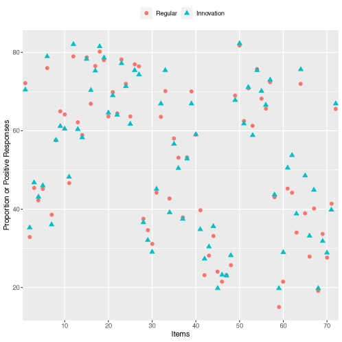
Figure 1: The proportion of positive responses for each of the 72 test items across all students of regular and innovation schools. The labels of the horizontal and vertical axes indicate item numbers.

To evaluate students’ non-cognitive outcomes, we selected 10 psychological/attitude scales that include Mental Ill-being (Item 1 - 6), Sense of Citizenship (Item 7 - 22), Self-Efficacy (Item 23 - 30, 71), Disbelief in Growth (Item 31 - 33), Self-Driven Learning (Item 34 - 37), Self-Understanding (Item 38 - 41), Test Stress (Item 42 - 48), Relationship with Friends (Item 49 - 54), Self-Esteem (Item 55 - 58, 72), and Academic Stress (Item 59 - 70). These are not established scales; hence, the trait measurements from these scales may be theoretically nonequivalent to the traits implied by the scale names. Each scale includes three to thirteen items that are measured with a five-point agreement-based Likert scale. All items are presented in the supplementary materials (Section A). Some of the items were negatively worded, and in that case we reverse-coded the responses to facilitate the interpretation of results (Items 1–6, 20–22, 31–33, 42–48, and 58–70). The responses from all individual items were then dichotomized such that 1 represents positive responses (“agree”) while 0 represents negative responses (“disagree”) for the data analysis.

Figure 1 displays the proportion of positive responses for each of the 72 test items across all students within the regular and innovation school systems. The figure shows that the degree and direction of the differences in the proportion scores widely varied across individual items. This suggests that univariate analysis using a summary score (e.g., mean, sum) can be misleading as such variation may be lost during the summarizing process. In addition, as aforementioned, the 72 items are from 10 different scales that measure related, but different psychological or attitudinal attributes of the students. All items are likely to be correlated with each other in varying degrees, while such correlation structures may differ between the two school systems. We propose a method that does not assume that all items have the same threshold levels and that the items are independent of each other.

Scope and goal of the data analysis

To analyze the GEPS data, we use all 72 items without distinguishing between scales, which is reasonable as the scales are not well-established scales but working scales. Our proposed approach explores similarities and dissimilarities of items and identifies clusters of items based on similarities and dissimilarities of the items. It is worth noting that we that do not discuss the sources of the differences between the school systems nor provide causal explanations. Causal inference based on observational data is non-trivial and is beyond the scope of our paper. Our data analysis is an exploratory approach aiming to identify differences between the two school systems, without attempting to make causal statements.

3 Multilevel network item response model

We introduce a multilevel network item response model with a view to analyzing the GEPS data, building on latent space models. To prepare the ground for the proposed modeling framework, we first provide a concise introduction to latent space models in Section 3.1 and then introduce the proposed modeling framework in Section 3.2. Throughout, we denote the set of real numbers by $\mathbb{R}$ and the set of positive real numbers by $\mathbb{R}_{+}$. The Euclidean distance between two vectors $\bm{a}$ and $\bm{b}$ in $\mathbb{R}^{q}$ is denoted by

$$\begin{array}[]{lllllllllllll}\displaystyle d(\bm{a},\,\bm{b})&=&\sqrt{\displaystyle\sum_{i=1}^{q}(a_{i}-b_{j})^{2}},&\;\bm{a}\in\mathbb{R}^{q},&\bm{b}\in\mathbb{R}^{q},&q\geq 1.\end{array}$$

3.1 Latent space models

The idea of embedding data into Euclidean space has a long history in educational statistics and related areas, as demonstrated by multidimensional scaling (e.g., Torgerson, 1952, 1965; Oh and Raftery, 2001, 2007). In recent decades, the idea of embedding data into Euclidean space has been adapted to network data represented by a graph with connections among nodes (Hoff et al., 2002). Known as latent space models, the basic idea is that nodes $i$ and $j$ have positions $\bm{z}_{i}$ and $\bm{z}_{j}$ in $\mathbb{R}^{q}$ and the probability of a connection $Y_{i,j}\in\{0,1\}$ between $i$ and $j$ depends on the distance $d(\bm{z}_{i},\,\bm{z}_{j})$ between them:

$$\begin{array}[]{lllllllllllll}\displaystyle Y_{i,j}\mid\beta,\,d(\bm{z}_{i},\,\bm{z}_{j})&\mathop{\rm\sim}\limits^{\mbox{\tiny ind}}&\mbox{Bernoulli}(\mathbb{P}(Y_{i,j}=1\mid\beta,\,d(\bm{z}_{i},\,\bm{z}_{j}))),\end{array}$$

where

$$\begin{array}[]{lllllllllllll}\displaystyle\log\displaystyle\frac{\mathbb{P}(Y_{i,j}=1\mid\beta,\,d(\bm{z}_{i},\,\bm{z}_{j}))}{1-\mathbb{P}(Y_{i,j}=1\mid\beta,\,d(\bm{z}_{i},\,\bm{z}_{j}))}&=&\beta-d(\bm{z}_{i},\,\bm{z}_{j}).\end{array}$$

In other words, the log odds of a connection between nodes $i$ and $j$ is $\beta\in\mathbb{R}$ when the distance $d(\bm{z}_{i},\,\bm{z}_{j})$ separating $i$ and $j$ in $\mathbb{R}^{q}$ is $0$, and is otherwise $\beta-d(\bm{z}_{i},\,\bm{z}_{j})$. Thus, the greater the distance separating nodes $i$ and $j$ in $\mathbb{R}^{q}$ is, the lower is the log odds of a connection between them. It is a convention to choose the dimension $q$ of $\mathbb{R}^{q}$ to be 2 or 3, to facilitate 2- or 3-dimensional representations of nodes in $\mathbb{R}^{2}$ or $\mathbb{R}^{3}$, respectively. If the random graph represents a social network, the latent space may be interpreted as an unobserved social space underlying the observed network of interactions. More background on latent space models can be found in, e.g., Hoff et al. (2002); Schweinberger and Snijders (2003); Handcock et al. (2007); Krivitsky et al. (2009); Raftery et al. (2012); Salter-Townshend et al. (2012); Sweet et al. (2013); Salter-Townshend and Murphy (2013); Tang et al. (2013); Sussman et al. (2014); Sewell and Chen (2015a, b, 2017); Fosdick and Hoff (2015); Rastelli et al. (2016); Gollini and Murphy (2016); Smith et al. (2019); and Ma et al. (2020).

3.2 Proposed modeling framework

We first review models of individual schools and then discuss multilevel extensions.

To introduce models of individual schools, we follow Jin and Jeon (2019) and introduce two sets of networks that represent similarities of students and items in a school of interest, and then adapt the approach of Jin and Jeon (2019) to multilevel data – that is, data from multiple schools. Consider $M$ schools $1,\dots,M$, with responses $X_{m,i,k}\in\{0,1\}$ to items $i\in\{1,\dots,p\}$ ($p\geq 1$) by students $k\in\{1,\dots,n_{m}\}$ ($n_{m}\geq 1$) in school $m\in\{1,\dots,M\}$ ($M\geq 1$). We consider two sets of networks, depending on whether embedding students or items in $\mathbb{R}^{q}$ is of primary interest:

• If embedding students in $\mathbb{R}^{q}$ is of primary interest, construct networks $\bm{Y}_{m,i}$ as follows ($i=1,\dots,p$,  $m=1,\dots,M$):

  $$\bm{Y}_{m,i}\;=\;(Y_{m,i,k,l})\;=\;(X_{m,i,k}\,X_{m,i,l}),$$

  where $Y_{m,i,k,l}=1$ indicates that students $k$ and $l$ in school $m$ both agree with item $i$.

• If embedding items in $\mathbb{R}^{q}$ is of primary interest, construct networks $\bm{U}_{m,k}$ as follows ($k=1,\dots,n_{m}$,  $m=1,\dots,M$):

  $$\bm{U}_{m,k}\;=\;(U_{m,k,i,j})\;=\;(X_{m,i,k}\,X_{m,j,k}),$$

  where $U_{m,k,i,j}=1$ indicates that student $k$ in school $m$ agrees with both items $i$ and $j$.

These networks are all undirected, in the sense that connections in these networks do not have directions. It is worth noting that there is more than one approach to constructing networks. The construction of networks described above makes some sense, in that students are embedded based on shared agreements with items, whereas items are embedded based on shared agreements by individual students. That being said, there are other possible constructions of networks: e.g., to embed items, one could construct networks $\bm{U}_{m,k}^{\star}$ by definining

$$\begin{array}[]{lllllllllllll}\displaystyle U_{m,k,i,j}^{\star}&=&X_{m,i,k}\,X_{m,j,k}+(1-X_{m,i,k})\,(1-X_{m,j,k}),\end{array}$$

in which case items $i$ and $j$ would be considered similar if student $k$ in school $m$ either agreed with both items or disagreed with both items. Indeed, one of the advantages of the proposed modeling framework is its flexibility in the construction of networks, which allows researchers to embed either items or students based on similarity measures of interest.

Embedding students based on latent space models of $\bm{Y}$’s

Students can be embedded in $\mathbb{R}^{q}$ by assuming that students $k$ and $l$ have positions $\bm{z}_{m,k}$ and $\bm{z}_{m,l}$ in $\mathbb{R}^{q}$ and that, conditional on the distance $d(\bm{z}_{m,k},\,\bm{z}_{m,l})$ separating students $k$ and $l$ in $\mathbb{R}^{q}$, the random variables $Y_{m,i,k,l}$ are independent Bernoulli random variables, with log odds

$$\begin{array}[]{lllllllllllll}\displaystyle\log\frac{\mathbb{P}(Y_{m,i,k,l}=1\mid\beta_{m,i},\,d(\bm{z}_{m,k},\,\bm{z}_{m,l}))}{1-\mathbb{P}(Y_{m,i,k,l}=1\mid\beta_{m,i},\,d(\bm{z}_{m,k},\,\bm{z}_{m,l}))}&=&\beta_{m,i}-d(\bm{z}_{m,k},\,\bm{z}_{m,l}).\end{array}$$ (1)

The parameter $\beta_{m,i}\in\mathbb{R}$ can be interpreted as the log odds that both students $k$ and $l$ in school $m$ agree with item $i$, provided that $k$ and $l$ are separated by distance $d(\bm{z}_{m,k},\,\bm{z}_{m,l})=0$. Otherwise, the log odds is reduced by the distance between students $k$ and $l$.

Embedding items based on latent space models of $\bm{U}$’s

Along the same lines, items can be embedded in $\mathbb{R}^{q}$ by assuming that items $i$ and $j$ have positions $\bm{w}_{m,i}$ and $\bm{w}_{m,j}$ in $\mathbb{R}^{q}$ and that, conditional on the distance $d(\bm{w}_{m,i},\,\bm{w}_{m,j})$ separating items $i$ and $j$ in $\mathbb{R}^{q}$, the random variables $U_{m,k,i,j}$ are independent Bernoulli random variables, with log odds

$$\begin{array}[]{lllllllllllll}\displaystyle\log\frac{\mathbb{P}(U_{m,k,i,j}=1\mid\theta_{m,k},\,d(\bm{w}_{m,i},\,\bm{w}_{m,j}))}{1-\mathbb{P}(U_{m,k,i,j}=1\mid\theta_{m,k},\,d(\bm{w}_{m,i},\,\bm{w}_{m,j}))}&=&\theta_{m,k}-d(\bm{w}_{m,i},\,\bm{w}_{m,j}).\end{array}$$ (2)

The parameter $\theta_{m,k}\in\mathbb{R}$ corresponding to student $k$ in school $m$ is the log odds that student $k$ agrees with both items $i$ and $j$ when items $i$ and $j$ are separated by distance $d(\bm{w}_{m,i},\,\bm{w}_{m,j})=0$. Otherwise, the log odds is reduced by the distance between items $i$ and $j$.

Joint probability model of $\bm{Y}$’s and $\bm{U}$’s

It is worth noting that the latent space models described above are proper probability models of the $\bm{Y}$’s and $\bm{U}$’s, but it is not straightforward to construct a joint probability model of the $\bm{Y}$’s and $\bm{U}$’s: e.g., it is not possible to construct a joint probability model of the $\bm{Y}$’s and $\bm{U}$’s by assuming that the $\bm{Y}$’s and $\bm{U}$’s are conditionally independent given the positions of students and items in $\mathbb{R}^{q}$, because the $\bm{Y}$’s and $\bm{U}$’s are deterministic functions of $\bm{X}$. That said, we are free to use the latent space models described above to embed either students or items in $\mathbb{R}^{q}$. If it is desired to embed both students and items in $\mathbb{R}^{q}$ to shed light on how students interact with items, the recent approach of Jeon et al. (2021) can be used.

Identifiability issues

The described latent space models have the same identifiability issues as other latent space models, rooted in the invariance of Euclidean distances to translation, reflection, and rotation of the positions of students and items in $\mathbb{R}^{q}$. As a consequence, the log odds (1) and (2) are invariant to these transformations, as is the resulting likelihood function. We follow the conventional approach to addressing these identifiability issues by basing statistical inference on equivalence classes of positions, using Procrustes matching (Hoff et al., 2002).

Selecting the dimension $q$ of $\mathbb{R}^{q}$

In principle, the dimension $q$ of $\mathbb{R}^{q}$ can be determined by model selection criteria, such as Bayesian information criteria (Handcock et al., 2007), although the theoretical properties of Bayesian information criteria in applications to latent space models are not well-understood. We therefore follow convention and choose $q=2$ (Hoff et al., 2002), which has advantages in terms of model parsimony and visualization.

Multilevel extensions

To discuss a simple multilevel extension of the latent space models introduced above, suppose that it is desired to embed items in $\mathbb{R}^{q}$ and combine the results across the $M$ schools. To combine the results across the $M$ schools and embed the $M$ schools in $\mathbb{R}^{q}$ along the way, construct a $M\times M$ matrix $\bm{\Delta}$ of dissimilarities $\bm{\Delta}_{a,b}=\sqrt{\sum_{i<j}^{p}(d_{a,i,j}-d_{b,i,j})^{2}}$ between schools $a$ and $b$, where $d_{m,i,j}$ refers to the distance $d(\bm{w}_{m,i},\,\bm{w}_{m,j})$ between items $i$ and $j$ in school $m\in\{1,\dots,M\}$. We can then embed the $M$ schools in $\mathbb{R}^{q}$ based on how dissimilar the schools are in terms of item responses by students, by applying Kruskal’s multidimensional scaling procedure to the dissimilarity matrix $\bm{\Delta}$ (Kruskal, 1964; Cox and Cox, 2001). The resulting procedure has the advantage that it requires nothing more than postprocessing the posterior samples of the $M$ schools and is therefore a simple alternative to random effects approaches to multilevel models, and provides an embedding of schools in $\mathbb{R}^{q}$.

3.3 Priors

We use the following priors. The hyperparameters of these priors are specified in Section 4.

Item parameters

Let $\bm{\beta}_{m}=(\beta_{m,1},\cdots,\beta_{m,p})\in\mathbb{R}^{p}$ denote the item parameter vector specific to school $m$ ($m=1,\cdots,M$). We assume that the $M$ item parameter vectors $\bm{\beta}_{1},\cdots,\bm{\beta}_{M}$ are independent, with prior

$$\begin{array}[]{lllllllllllll}\displaystyle\beta_{m,i}\mid\sigma_{\beta}^{2}&\mathop{\rm\sim}\limits^{\mbox{\tiny iid}}&N(0,\,\sigma_{\beta}^{2}),\end{array}$$

where $\sigma_{\beta}^{2}\in\mathbb{R}_{+}$ is a specified hyperparameter.

Student parameters

Let $\bm{\theta}_{m}=(\theta_{m,1},\cdots,\theta_{m,n_{m}})\in\mathbb{R}^{n_{m}}$ denote the student parameter vector specific to school $m$ ($m=1,\cdots,M$). We assume that the $M$ student parameter vectors $\bm{\theta}_{1},\cdots,\bm{\theta}_{M}$ are independent, with prior

$$\begin{array}[]{lllllllllllll}\displaystyle\theta_{m,k}\mid\sigma_{\theta}^{2}&\mathop{\rm\sim}\limits^{\mbox{\tiny iid}}&N(0,\,\sigma_{\theta}^{2}),\end{array}$$

where $\sigma_{\theta}^{2}\in\mathbb{R}_{+}$ is a specified hyperparameter.

Item distances

Let $d_{m,i,j}\equiv d(\bm{w}_{m,i},\,\bm{w}_{m,j})$ be the distance between items $i$ and $j$ in school $m$, and let $\bm{D}_{m}=(d_{m,i,j})$ be the $p\times p$ matrix of distances between items in school $m$ ($m=1,\dots,M$). We allow variation across the $M$ schools by using the following prior:

$$\begin{array}[]{lllllllllllll}\displaystyle d_{m,i,j}\mid\mu_{i,j},\,\tau_{i,j}^{2}&\mathop{\rm\sim}\limits^{\mbox{\tiny ind}}&\mbox{Lognormal}(\mu_{i,j},\,\tau_{i,j}^{2}),\;\;\;\;i<j\in\{1,\dots,p\}\vspace{.25cm}\\ \mu_{i,j}\mid\sigma_{\mu}^{2}&\mathop{\rm\sim}\limits^{\mbox{\tiny iid}}&N(0,\,\sigma_{\mu}^{2})\vspace{.25cm}\\ \tau_{i,j}^{2}\mid a_{\tau},\,b_{\tau}&\mathop{\rm\sim}\limits^{\mbox{\tiny iid}}&\mbox{Inverse-Gamma}(a_{\tau},\,b_{\tau}),\end{array}$$

where $\sigma_{\mu}^{2}\in\mathbb{R}_{+}$, $a_{\tau}\in\mathbb{R}_{+}$ and $b_{\tau}\in\mathbb{R}_{+}$ are specified hyperparameters. The collections of means $\mu_{i,j}$ and variances $\tau_{i,j}^{2}$ are denoted by $\bm{\mu}$ and $\bm{\tau}$, respectively. In addition to the single-group model described above, we consider a multiple-group model, which allows the means and variances to depend on the regular and innovation school system. It is worth noting that the prior of the distances specified above is a convenience prior, covering distances (which satisfy the triangle inequality) along with non-distances (which do not satisfy the triangle inequality). While the prior is motivated by convenience, it does cover the space of interest (the space of all distances) and the Bayesian algorithm described in Section 3.4 with postprocessing procedures (a) and (b) reports distances between items (satisfying the triangle inequality). The use of convenience priors is not unprecedented in Bayesian statistics: e.g., uniform priors may not reflect prior knowledge and may not even be proper priors, but can give rise to proper posteriors and can be useful in applications (e.g., Taraldsen and Lindqvist, 2010).

3.4 Bayesian inference

We follow a Bayesian approach to estimating the multilevel network item response model and focus on embedding items in $\mathbb{R}^{q}$ along with schools, motivated by the application to the GEPS data.

Posterior

To embed items in $\mathbb{R}^{q}$ along with schools, compute the networks $\bm{U}_{m,k}=(U_{m,k,i,j})$ by computing $U_{m,k,i,j}=X_{m,i,k}\,X_{m,j,k}$ and write $\bm{U}_{m}=(\bm{U}_{m,1},\dots,\bm{U}_{m,n_{m}})$ ($m=1,\dots,M$). Then the posterior of $\bm{\theta}_{1},\dots,\bm{\theta}_{M}$ and $\bm{D}_{1},\dots,\bm{D}_{M}$ given $\bm{U}_{1},\dots,\bm{U}_{M}$ is proportional to

$$\begin{array}[]{lllllllllllll}\displaystyle\pi(\bm{\theta}_{1},\dots,\bm{\theta}_{M},\,\bm{D}_{1},\dots,\bm{D}_{M}\mid\bm{U}_{1},\dots,\bm{U}_{M})&\propto&\left[\displaystyle\prod_{m=1}^{M}\,\displaystyle\prod_{k=1}^{n_{m}}\,\displaystyle\prod_{i<j}^{p}\,\mathbb{P}(U_{m,k,i,j}=u_{m,k,i,j}\mid\theta_{m,k},\,d_{m,i,j})\right]\vspace{.25cm}\\ &\times&\left[\displaystyle\prod_{m=1}^{M}\,\pi(\bm{\theta}_{m})\;\pi(\bm{D}_{m}\mid\bm{\mu},\,\bm{\tau})\right]\;\pi(\bm{\mu})\;\pi(\bm{\tau}),\end{array}$$

where $\bm{D}_{m}=(d_{m,i,j})$ and $d_{m,i,j}$ refers to $d(\bm{w}_{m,i},\,\bm{w}_{m,j})$ ($m=1,\dots,M$).

Markov chain Monte Carlo algorithm

A Markov chain Monte Carlo algorithm for sampling from the posterior distribution can then be constructed by combining the following Markov chain Monte Carlo steps, assuming all unknown quantities have been initialized.

1. Preprocessing: Construct $\bm{U}_{1},\dots,\bm{U}_{M}$.

2. Iterate:

3. Sample the positions of items and the parameters of school $m$, where $\bm{w}_{m,-i}$ refers to the positions of all items excluding $\bm{w}_{m,i}$ and $\bm{\theta}_{m,-k}$ refers to all parameters excluding $\theta_{m,k}$ ($m=1,\dots,M$):

   1. Sample $\bm{w}_{m,i}\mid\bm{U}_{m},\,\bm{w}_{m,-i},\,\bm{\theta}_{m},\,\bm{\mu},\,\bm{\tau}^{2}$ ($i=1,\dots,p$,  $m=1,\dots,M$).

   2. Sample $\theta_{m,k}\mid\bm{U}_{m},\,\bm{\theta}_{m,-k},\,\bm{w}_{m,1},\,\dots,\,\bm{w}_{m,p}$ ($k=1,\dots,n_{m}$, $m=1,\dots,M$).

4. Sample the hyperparameters:

   1. Sample $\mu_{i,j}\mid d(\bm{w}_{1,i},\,\bm{w}_{1,j}),\cdots,d(\bm{w}_{M,i},\,\bm{w}_{M,j}),\,\tau_{i,j}^{2}$.

   2. Sample $\tau_{i,j}^{2}\mid d(\bm{w}_{1,i},\,\bm{w}_{1,j}),\cdots,d(\bm{w}_{M,i},\,\bm{w}_{M,j}),\,\mu_{i,j}$.

5. Postprocessing:

   • To solve the identifiability issue arising from the invariance of the likelihood function to reflection, translation, and rotation of the item positions, use Procrustes matching.

   • To embed the $M$ schools in $\mathbb{R}^{q}$, construct a $M\times M$ matrix $\bm{\Delta}$ of dissimilarities$\bm{\Delta}_{a,b}=\sqrt{\sum_{i<j}^{p}(d_{a,i,j}-d_{b,i,j})^{2}}$ between schools $a$ and $b$, where $d_{m,i,j}$ refers to the distance $d(\bm{w}_{m,i},\,\bm{w}_{m,j})$ between items $i$ and $j$ in school $m\in\{1,\dots,M\}$ obtained in Step (a). Then embed the $M$ schools in $\mathbb{R}^{q}$ by applying Kruskal’s multidimensional scaling procedure to the dissimilarity matrix $\bm{\Delta}$.

We used Metropolis-Hasting algorithms for updating the positions of items and the parameters, and Gibbs sampling for updating the hyperparameters. Section B of the supplement provides additional details of the MCMC algorithm.

Remark. The postprocessing procedures (a) and (b) are motivated in Section 3.2. In Step (a), we follow the conventional approach to addressing the identifiability issues of latent space models by basing statistical inference on equivalence classes of positions, using Procrustes matching (Hoff et al., 2002). In Step (b), note that the matrix $\bm{\Delta}$ consists of dissimilarities rather than distances between schools, because there is no guarantee that the dissimilarities of schools satisfy the triangle inequality. That said, Kruskal’s procedure accepts dissimilarities as input and produces distances as output. In other words, the procedure described above produces an embedding of schools in $\mathbb{R}^{q}$, despite the fact that the matrix $\bm{\Delta}$ consists of dissimilarities rather than distances.

3.5 Relations to existing approaches

A multilevel latent space model (Sweet et al., 2013) has been proposed to handle school-level clustering for social network data, by including a random effect in a standard latent space model to capture variation across schools. In our proposed approach, we take one step further and construct a school-level latent space, providing additional and more in-depth information on how schools are similar or different from each other in terms of their item or student network structures. Our multilevel network item response model simultaneously analyzes three types of networks, at the item, student, and school levels, based on multilevel item response data. Thus, the proposed model is a unique statistical tool that can identify three different types of sub-grouping (or clustering) structures that may be present at the item, student, and school levels.

In addition, our approach has advantages over conventional latent variable modeling approaches. For example, multilevel exploratory item factor analysis (MEFA; Muthen, 1994) can identify clustering of items, i.e., factor structure, at a lower-level unit (within-group such as students) and at a higher-level unit (between-group such as schools); but MEFA cannot identify clustering of students and clustering of schools. Multilevel mixture IRT models (MMIRT; Vermunt, 2003) can identify clustering of students and schools in terms of how the item parameters differ across clusters; however, clustering of items may be unidentifiable at the same time. Alternatively, a multilevel item response theory (MIRT) model or a multilevel SEM model (MSEM) may be considered. Both MIRT and MSEM may offer information on how schools differ in terms of school-level average scores. In contrast, our approach helps us examine how schools are different in terms of how individual students responded to individual test items. We demonstrated in Section 4.3 that an MIRT is unable to detect the differences among schools that our approach is able to detect with the GEPS data.

4 Analysis and results

4.1 Method

We apply the latent space model described in Section 3 to the GEPS data described in Section 2. We assume that items have positions in $\mathbb{R}^{2}$ and approximate the posterior by using the Markov chain Monte Carlo algorithm described in Section 3.4. To detect possible non-convergence of the Markov chain Monte Carlo algorithm, we ran the Markov chain Monte Carlo algorithm five times, with starting values chosen at random. Each Markov chain Monte Carlo run consisted of 50,000 iterations, with the first 25,000 iterations discarded as a burn-in. From the remaining 25,000 iterations, 2,500 samples were collected by retaining every tenth draw from the posterior. We set $\sigma_{\theta}=\sigma_{\mu}=10$ and $a_{\tau}=b_{\tau}=.01$. Trace plots of draws from the posterior can be found in the supplementary materials (Section D). The differences between the five Markov chain Monte Carlo runs were negligible and the standard errors were less than $.05$ for all quantities.

4.2 Model Fit

To evaluate model fit, we examined the predictive power of the model. The idea was to predict adjacency matrices $\bm{U}$ based on the estimated model parameters—estimated by posterior means—and evaluate the predictive power of the estimated model in terms of sensitivity and specificity. It is worth noting that these predictive checks are not strictly posterior predictive checks in the Bayesian sense, but have the advantage of being less computation-intensive. These posterior predictions are in-sample predictions, as is common in the literature on statistical network models, including latent space models.

To evaluate predictive power of the proposed model, we defined sensitivity as TF/(TF + FN) and specificity as TN/(TN + FP), where TF: true negative, FN: false negative, TN: true negative, and FP: false positive. We also computed the overall accuracy as (TP + TN) / (TP + TN + FP + FN), where TP: true positive, TN: true negative, FP: false positive, and FN: false negative. We found that the sensitivity, specificity, and overall accuracy of the proposed model turned out to be satisfying for $\bm{U}$ with a sensitivity of 0.45 and a specificity of 0.82, and an overall accuracy was 0.710. We provide the sensitivity, specificity, and overall accuracy of individual schools in the supplementary materials (Section E). Taken together, the model fit assessment results suggest the predictive power, and thus, the fit of the estimated model was reasonable for the GEPS data.

4.3 Results

We discuss results, with an emphasis on how the innovation and regular school systems were different in terms of item network and school network structures. We do not discuss student network structures here for the sake of parsimony; comparing within-school student network structures across all schools is not practical due to the large sample size. Plus, school-level network structures supply a sensible summary of student network structures across schools. A summary of the person parameter estimates is provided in the supplement (Section C).

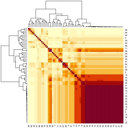
Figure 2: Heatmap based on the estimated $\bm{\mu}=(\mu_{i,j})$ obtained from the single-group model. Numbers represent items.

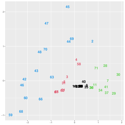
Figure 3: Embedding of items in $\mathbb{R}^{2}$ based on the single-group model. Numbers represent items. Colors represent the clusters estimated from the dendrogram in Figure 2.

Item network structure

Figure 2 shows a heatmap of $\bm{\mu}$ from the single-group model (see “Item distances” in Section 3.3). The heatmap shows that a bulk of items is concentrated in a small region of the $\mathbb{R}^{2}$ space. While most other items are not too far away from this item bulk, some are fairly distant from them. Those distant nodes, though, did not cause any computational problem (the minimum proportion of “agree” was 16.1% for Item 59).

(a) Regular schools

(b) Innovation schools

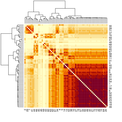
Figure 4: Heatmaps based on the estimated $\bm{\mu}=(\mu_{i,j})$ obtained from the multiple-group model: (a) Regular schools and (b) Innovation schools. Numbers represent items.

(a) Regular Schools	(b) Innovation Schools

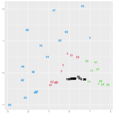
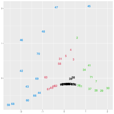
Figure 5: Embedding items in $\mathbb{R}^{2}$ based on the multiple-group model: (a) Regular schools and (b) Innovation schools. Numbers represent items. Colors represent the clusters estimated from the dendrograms in Figure 4.

Figure 3 shows the latent space of the test items, constructed by applying MDS to $\bm{\mu}$. The numbers in black correspond to the item bulk discussed above with Figure 2; these items are located near the origin (0,0) of the $\mathbb{R}^{2}$ space, meaning that a majority of students in the data positively endorsed the items in this group, which measure “Sense of Citizenship”,“Self-Efficacy”, “Relationship with Friends”, and “Self-Esteem”. In the latent space, we differentiated three item groups identified from the dendrogram (shown in Figure 2) in three different colors. The items in green, placed in the east of the items in black, include several items measuring “Self-efficacy” and items measuring “Sense of Citizenship ” (I7), “Self-driven Learning (I37), and “Self-understanding” (I41). The items in red, located to the west of the items in black, include items that measure “Academic stress” and “Mental well-being”. The items in blue, spread in the far east of the black-numbered items, include items measuring “Test stress” and “Academic stress”.

From the multiple group model, we obtained two separate item network structures for innovation and regular school systems, which enables us to investigate differences in the item network structure between the two school systems. Figures 4 and 5 show the results. The two space configurations are nearly identical, except for two items – Item 2 (“I am worried about everything.”) is in blue in the regular schools but in green in the innovation schools, and Item 63 (“If you talk to your parents about my study, you get irritated rather than stable.”) is in blue in the regular schools but in red in the innovation schools. The result suggests that overall, the response patterns of the students are nearly indistinguishable between the two school types.

School network structure

(a)

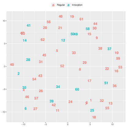
(b)

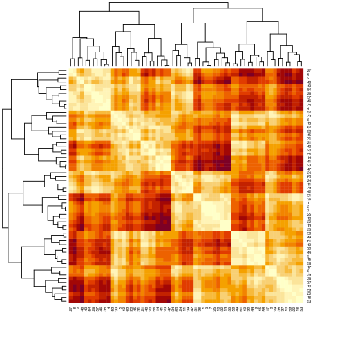
Figure 6: (a) Latent positions of individual schools constructed by the school-specific mean of the between-item distance measures $\Delta$. The procedure for embedding schools in $\mathbb{R}^{2}$ is described in Section 3.3. (b) A heatmap based on the estimated $\Delta$.

Figure 6(a) shows the latent space of the schools obtained based on $\Delta$, red and blue representing regular schools and innovation schools, respectively. Overall, the 62 schools are widely spared out in the school latent space, but the locations of the innovation schools and the regular schools are rather mixed than separated from each other. The difference in the school latent positions reflect differences in the item dependence structures between schools. Thus, the results indicate that the two school systems are not clearly distinguishable in terms of the item dependence structures, suggesting that the school type (innovation vs. regular) might not be a main deriving factor that explains school differences in the relationships between the test items (which is the result of how students responded to the test items).

The dendrogram in Figure 6(b) shows four school clusters: a upper-left group, a upper-right group, a bottom-left group, and a bottom-right group. For close inspection, we picked one school from each cluster: Schools 1, 2, 56, and 10, respectively. Schools 10 and 2 are far away from each other, located at the north-east side and south-west side of the latent space. Schools 56 an 1 are also far apart from each other, located at the north-west side and south-east side of the space. School 2 is the only innovation school among the four selected schools.

Figure 7 presents the item latent spaces of the four selected schools. The item latent spaces of all other schools are provided in the supplementary materials (Section F). It is interesting that a virtual line may be drawn from Item 59 to Item 29 (from top left to bottom right) in all four latent spaces; and items near the virtual line are nearly identical in the four latent spaces. However, the positions of most other items outside this line appear different in the four latent spaces. For example, items on the east to the origin (e.g., Items 2, 3, 11, 30, 42, 44, 45, 48, 69, 70, 71) are positioned differently in Schools 2 and 10, meaning that the relationship between the items, in other words, how students conceived and responded to those items were different in the two schools.

(a) School 10	(b) School 1
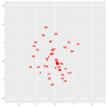
(c) School 2	(d) School 56

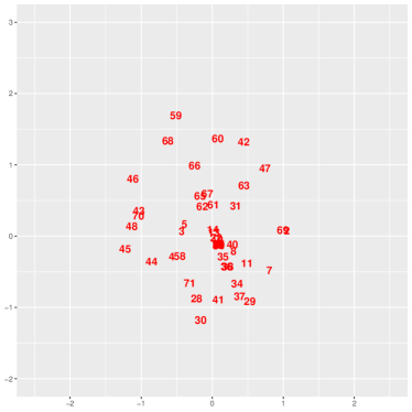
Figure 7: Student and item latent spaces for Schools 1, 2, 10, and 56. Red numbers represent item latent positions, respectively.

For a better understanding of the school-specific latent spaces examined above, we checked the proportion of “agree” (positive responses) of the two schools, School 2 and 10 in Figure 7. As expected, the figure shows that there are notable differences between the two schools in terms of how students responded to the test items. Overall, the proportion of positive responses appears higher in School 2 than School 10 for most items, while for some item, such as Items 2–6, 28–30, 45, 70, the proportion of “agree” is higher in School 10 than School 2. Those items measure sense of citizenship, self-efficacy and reverse-coded academic stress, and they roughly correspond to the items that are positioned differently in the school-specific latent spaces shown in Figure 7. This inspection shows that schools located in different regions of the school-specific latent space are indeed different in terms of their students’ response patterns.

All in all, our analysis results tell us that there are substantial differences across schools in terms of how the students conceived and responded to items measuring their mental well-being, but the differences were not necessarily driven by whether or not the schools adopted the innovation school system.

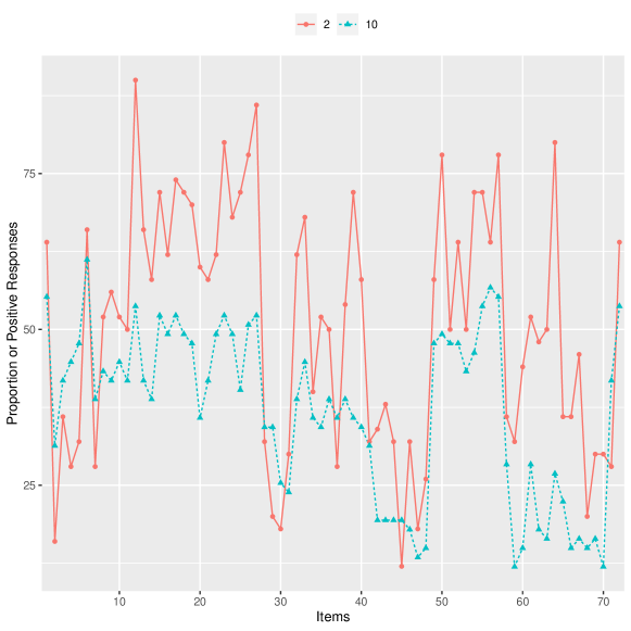
Figure 8: Proportion of “agree” across 72 items in Schools 2 and 10.

Comparison: multilevel Rasch model

We applied a multilevel Rasch model to the GEPS data, with the school program as a school-level covariate, to compare our approach to a conventional approach. We chose a multilevel Rasch model for a comparison because this model assumes the same latent variable structure (with a single latent variable) at the student level as the estimated model, and allows us to make inferences about differences in student responses between the two school types of interest. A multilevel Rasch model posits that the log odds of the probability of a positive response by student $k$ in school $m$ to item $i$ is

$$\begin{array}[]{lllllllllllll}\displaystyle\mbox{logit}(\mathbb{P}(X_{m,i,k}=1\mid\beta_{i},\,\gamma,\,\delta_{m},\,\theta_{m,k})&=&\beta_{i}+\gamma\;I_{m}+\delta_{m}+\theta_{m,k},\end{array}$$

where $\beta_{i}\in\mathbb{R}$ and $\delta_{m}\in\mathbb{R}$ are the item-specific and school-specific intercepts and $\theta_{m,k}\in\mathbb{R}$ are the student- and school-item-specific effects, respectively. The parameter $\gamma\in\mathbb{R}$ represents the deviation of the Innovation schools’ effects from the regular schools’ effects (where $I_{m}$ represents the binary indicator for innovation schools).

The multilevel Rasch model specified above was estimated by Bayesian Markov chain Monte Carlo methods, using R package MCMCglmm (Hadfield, 2010) with 13,000 iterations, 3,000 burn-in iterations, and recording every $10$-th draw from the posterior. There is little evidence that the two school programs differ in terms of the overall school means, because the 95% posterior credible interval is [-0.139, 0.301] (which includes $0$). The posterior means of school-specific intercept $\delta_{m}$ ranged from -1.27 to 0.82 across 62 schools with the mean of 0.01. The posterior means and 95% posterior credible intervals of the school-specific intercepts are -0.25 [-0.46, -0.01], and -1.27 [-1.42, -1.11] for School 2 and 10, respectively. That is, this result tells us that students in School 10 on average showed a lower level of mental well-being than students in School 10, without giving in-depth information about how the schools differ in terms of student responses to the well-being questions.

5 Conclusion

The Korean school innovation program, implemented in the last 9 years in Korea, has been under public scrutiny due to widespread skepticism about its effectiveness. Most research on the school innovation program has relied on simple comparison methods and produced mixed results about the programs’ effects on students’ non-cognitive outcomes, calling for a more comprehensive study that can shed new light on the issue.

Motivated by this need, we proposed a novel analytic approach that allows us to explore differences between the innovation and regular school programs from a fresh angle in terms of their students’ non-cognitive outcomes. The innovation of the proposed multilevel network modeling approach lies in that a latent space modeling technique, originally developed for network data, was adapted to analyze multilevel item response data for the purpose of examining networks (similarities and dissimilarities) of items, students, and schools, in addition to the item and student parameters. This method has not only technical advantages compared with traditional multilevel modeling methods, but also provides substantive merits by allowing us to investigate more subtle differences between innovation schools and regular schools than other methods cannot offer.

Upon an inspection on the item network structure of the GEPS data, we did not find strong evidence that innovation school students were distinguishable from regular school students in terms of the item network structure. That is, the students in the innovation school system were not different from the students in the regular school system in terms of how they conceived and responded to individual test items measuring positive self-image or mental well-being.

Even so, our approach did reveal that some schools were rather different from the others in terms of the item network structure, although the differences do not appear to stem from whether or not the schools adopted the innovation program. Those differences were not detected by conventional approaches, such as multilevel models, as shown in this paper.

It would be beneficial to apply a formal test to make a selection between the proposed model and simpler, multilevel models. However, due to the substantial differences in the basis and structure of the two kinds of models, developing a formal comparison test is a challenging task and it is beyond the scope of the current paper. Simpler alternatives such as multilevel models may have computational advantages over our approach. However, the proposed approach provides a unique opportunity to examine the differences between the two school types in the current context from a unique angle, in terms of how students responded differently to specific test items. For instance, suppose two schools were similar in terms of average student performance in a mathematics test; but in one school students performed better with calculation items than data analysis items, while in the other school, students performed better with data analysis items than calculation items. Therefore, despite potential computational cost, the proposed approach can be beneficial for the opportunity that enables us to make an in-depth investigation and comparisons among schools.

Source code and data

The R source code used in Section 4 can be found on GitHub:

https://github.com/Jonghyun-Yun/HiNIRM

The data cannot be shared without the consent of the government of South Korea. Interested readers are referred to the English-language website of the Gyeonggi Institute of Education in South Korea:

https://www.gie.re.kr/eng/content/C0012-04.do

Acknowledgements

We are grateful to two anonymous referees, the Associate Editor and the Editor for constructive comments and suggestions that have led to substantial improvements of the manuscript. Ick Hoon Jin was partially supported by the Yonsei University Research Fund of 2019-22-0210 and by Basic Science Research Program through the National Research Foundation of Korea (NRF 2020R1A2C1A01009881). Michael Schweinberger was partially supported by NSF awards DMS-1513644 and DMS-1812119 and ARO award W911NF-21-1-0237 (75549-NS). Lizhen Lin would like to acknowledge the general support from NSF grants IIS-1663870 and DMS-1654579 and Darpa grant N66001-17-1-4041.

References

- Bae (2014) Bae, E. J. (2014). Exploring the characteristics and conflicts of innovation school operation. Korean Journal of Educational Sociology 24, 145–180.
- Baek and Park (2014) Baek, B. B. and M. H. Park (2014). Analysis of innovation school performance: Focusing on reducing educational gap. Policy Research. 2014-14.
- Cho and Han (2016) Cho, M. G. and S.-Y. Han (2016). Exploring the influence of innovative schools on mental health through student-teacher relationships. The 3rd Gyeonggi Educational Research Projects Conference, Gyeonggi Provincial Education Research Institute.
- Cox and Cox (2001) Cox, T. F. and M. A. A. Cox (2001). Multidimensional Scaling. London: Chapman & Hall.
- Fosdick and Hoff (2015) Fosdick, B. K. and P. D. Hoff (2015). Testing and modeling dependencies between a network and nodal attributes. Journal of the American Statistical Association 110, 1047–1056.
- Gollini and Murphy (2016) Gollini, I. and T. B. Murphy (2016). Joint modeling of multiple network views. Journal of Computational and Graphical Statistics 25, 246–265.
- Gu et al. (2013) Gu, J.-U., H.-S. Bae, T.-H. Jung, J.-Y. Namgung, S.-A. Yoo, C.-H. Lee, K.-Y. Jung, G.-J. Choi, and E.-J. Huh (2013). Report on the results of the 2013 Seoul innovation school evaluation research project. Technical Report TR 2013-75.
- Gyeonggi Provincial Office of Education (2012) Gyeonggi Provincial Office of Education (2012). Plan of innovation school management. Republic of Korea: Gyeonggi Province.
- Hadfield (2010) Hadfield, J. D. (2010). MCMC methods for multi-response generalized linear mixed models: The MCMCglmm R package. Journal of Statistical Software 33(2), 1–22.
- Handcock et al. (2007) Handcock, M. S., A. E. Raftery, and J. M. Tantrum (2007). Model-based clustering for social network. Journal of the Royal Statistical Society, Series A 170, 301–354.
- Hoff et al. (2002) Hoff, P., A. Raftery, and M. S. Handcock (2002). Latent space approaches to social network analysis. Journal of the American Statistical Association 97, 1090–1098.
- Jang et al. (2014) Jang, J. H., J. S. Jung, and D. J. Won (2014). Comparison of structural relationships between school satisfaction, test stress, and academic achievement of innovative and regular school students. The 1st Gyeonggi Educational Research Projects Conference, Gyeonggi Provincial Education Research Institute.
- Jeon et al. (2021) Jeon, M., I. H. Jin, M. Schweinberger, and S. Baugh (2021). Mapping unobserved item-respondent interactions: A latent space item response model with interaction map. Psychometrika 86, 378–403.
- Jin and Jeon (2019) Jin, I. H. and M. Jeon (2019). A doubly latent space joint model for local item and person dependence in the analysis of item response data. Psychometrika 84(1), 236–260.
- Kim (2016) Kim, J. C. (2016). Changes in academic achievement and curriculum interests by school type. The 3rd Gyeonggi Educational Research Projects Conference, Gyeonggi Provincial Education Research Institute.
- Kim (2011) Kim, S. K. (2011). Analysis of actual conditions and performance of innovation school. The Korean Journal of Educational Administration 29, 145–168.
- Kim (2014) Kim, W. J. (2014). Influence of experience of student self-government activity on community consciousness: Comparison between innovation school and general school. The 1st Gyeonggi Educational Research Projects Conference, Gyeonggi Provincial Education Research Institute.
- Krivitsky et al. (2009) Krivitsky, P. N., M. S. Handcock, A. E. Raftery, and P. D. Hoff (2009). Representing degree distributions, clustering, and homophily in social networks with latent cluster random network models. Social Networks 31, 204–213.
- Kruskal (1964) Kruskal, J. (1964). Nonmetric multidimensional scaling: A numerical method. Psychometrika 29(2), 115–129.
- Lee et al. (2012) Lee, G., K. Y. Wu, S. C. Kim, H. D. Kim, and W. C. Seo (2012). Study of the performance and diffusion methods for innovation school programs. Gyeonggi Province Office of Education.
- Ma et al. (2020) Ma, Z., Z. Ma, and H. Yuan (2020). Universal latent space model fitting for large networks with edge covariates. Journal of Machine Learning Research 21, 1–67.
- Min et al. (2017) Min, K. S., H. Jung, and C. M. Kim (2017). Examining a causal effect of Gyeonggi innovation schools in Korea. KEDI Journal of Educational Policy 14, 3–20.
- Muthen (1994) Muthen, B. (1994). Multilevel covariance structure analysis. Sociological Methods & Research 22, 376–398.
- Nah (2013) Nah, M. J. (2013). Analysis of autonomous school performance: Focusing on innovative school programs. Korea Institute of Educational Development. CR 2013-10.
- Oh and Raftery (2001) Oh, M.-S. and A. Raftery (2001). Bayesian multidimensional scaling and choice of dimension. Journal of the American Statistical Association 96, 1031–1044.
- Oh and Raftery (2007) Oh, M.-S. and A. Raftery (2007). Model-based clustering with dissimilarities: A Bayesian approach. Journal of Computational and Graphical Statistics 16, 559–585.
- Raftery et al. (2012) Raftery, A., X. Niu, P. Hoff, and K. Yeung (2012). Fast inference for the latent space network model using a case-control approximate likelihood. Journal of Computational and Graphical Statistics 21, 909–919.
- Rastelli et al. (2016) Rastelli, R., N. Friel, and A. Raftery (2016). Properties of latent variable network models. Network Science 4, 407–432.
- Salter-Townshend and Murphy (2013) Salter-Townshend, M. and T. B. Murphy (2013). Variational Bayesian inference for the latent position cluster model for network data. Computational Statistics and Data Analysis 57, 661–671.
- Salter-Townshend et al. (2012) Salter-Townshend, M., A. White, I. Gollini, and T. B. Murphy (2012). Review of statistical network analysis: models, algorithms, and software. Statistical Analysis and Data Mining 5, 243–264.
- Schweinberger and Snijders (2003) Schweinberger, M. and T. A. B. Snijders (2003). Settings in social networks: A measurement model. Sociological Methodology 33, 307–341.
- Sewell and Chen (2015a) Sewell, D. K. and Y. Chen (2015a). Analysis of the formation of the structure of social networks by using latent space models for ranked dynamic networks. Journal of the Royal Statistical Society: Series C (Applied Statistics) 64, 611–633.
- Sewell and Chen (2015b) Sewell, D. K. and Y. Chen (2015b). Latent space models for dynamic networks. Journal of the American Statistical Association 110, 1646–1657.
- Sewell and Chen (2017) Sewell, D. K. and Y. Chen (2017). Latent space approaches to community detection in dynamic networks. Bayesian Analysis 12, 351–377.
- Smith et al. (2019) Smith, A. L., D. M. Asta, and C. A. Calder (2019). The geometry of continuous latent space models for network data. Statistical Science 34, 428–453.
- Sung et al. (2014) Sung, G., B. C. Minh, and J. E. Kim (2014). Analysis of the effectiveness of the innovation school system in gyeonggi province: Focused on elementary schools. The 1st Gyeonggi Educational Research Projects Conference, Gyeonggi Provincial Education Research Institute.
- Sussman et al. (2014) Sussman, D., M. Tang, and C. Priebe (2014). Consistent latent position estimation and vertex classification for random dot product graphs. IEEE Transactions on Pattern Analysis and Machine Intelligence 36, 48–57.
- Sweet et al. (2013) Sweet, T. M., A. C. Thomas, and B. W. Junker (2013). Hierarchical network models for education research: Hierarchical latent space models. Journal of Educational and Behavioral Statistics 38, 295–318.
- Tang et al. (2013) Tang, M., D. L. Sussman, and C. E. Priebe (2013). Universally consistent vertex classification for latent positions graphs. The Annals of Statistics 41, 1406–1430.
- Taraldsen and Lindqvist (2010) Taraldsen, G. and B. H. Lindqvist (2010). Improper priors are not improper. 64, 154–158.
- Torgerson (1952) Torgerson, W. S. (1952). Multidimensional scaling: I. Theory and method. Psychometrika 17, 401–419.
- Torgerson (1965) Torgerson, W. S. (1965). Multidimensional scaling of similarity. Psychometrika 30, 379–393.
- Vermunt (2003) Vermunt, J. K. (2003). Multilevel latent class models. Sociological Methodology 33, 213–239.