A Self-Organizing Tensor Architecture for Multi-View Clustering

Abstract

In many real-world applications, data are often unlabeled and comprised of different representations/views which often provide information complementary to each other. Although several multi-view clustering methods have been proposed, most of them routinely assume one weight for one view of features, and thus inter-view correlations are only considered at the view-level. These approaches, however, fail to explore the explicit correlations between features across multiple views. In this paper, we introduce a tensor-based approach to incorporate the higher-order interactions among multiple views as a tensor structure. Specifically, we propose a multi-linear multi-view clustering (MMC) method that can efficiently explore the full-order structural information among all views and reveal the underlying subspace structure embedded within the tensor. Extensive experiments on real-world datasets demonstrate that our proposed MMC algorithm clearly outperforms other related state-of-the-art methods.

I Introduction

In many applications, data are naturally comprised of multiple representations or views. For example, images on the web have textual descriptions associated with them; one document may be translated into multiple different languages. Observing that different views often provide compatible and complementary information, it appears natural to integrate them together for better performance rather than relying on a single view. The key of learning from multiple views is to leverage the interactions and correlations between views in order to outperform simply concatenating views. As multi-view data without labels are plentiful in real world applications, the problem of unsupervised learning from unlabeled multi-view data has attracted considerable attention in recent years [1, 2, 3], referred to as multi-view clustering.

Most of existing multi-view clustering algorithms are essentially extended from classical single-view clustering algorithms, such as spectral clustering and K-means clustering. For example, a co-regularized multi-view spectral clustering [4] is developed by keeping the consistency to the same clustering across all of similarity graphs. Some works [5, 6] adaptively learn weights to differ the reliability of different views for each graph during the optimization. Although these multi-view spectral clustering algorithms can achieve promising performance, they still have two main drawbacks: First, these algorithms generally need to build a proper similarity graph for each view. The construction of the similarity graph is a key issue involving many factors, such as the choice of kernels and their parameters. These factors may greatly affect the final clustering performance. Second, due to the heavy computation of similarity graphs, these graph based methods cannot effectively tackle large-scale multi-view clustering problems.

In contrast, multi-view K-means clustering approaches are more practically useful to deal with large-scale data since they are free from constructing similarity graphs. This kind of methods is originally derived from the non-negative matrix factorization (NMF) with orthogonality constraints, which is equivalent to relaxed K-means clustering [7]. [8] proposed a joint NMF based multi-view clustering algorithm via seeking for a factorization that gives compatible clustering solutions across multiple views.  [9] proposed the robust multi-view K-means clustering by using the structured sparsity-inducing norm, $\ell_{2,1}$-norm, to replace the Frobenius-norm in the K-means clustering objective and learning individual weight for each view. After [10] showed that a regression-like clustering objective is equivalent to the Discriminative K-means,  [11] incorporated the group $\ell_{1}$-norm together with the $\ell_{2,1}$-norm as joint structured regularization terms in the objective to better capture the view-wise relationships among data. However, these algorithms are performed in the original feature space without any discriminative subspace learning mechanism that may render curse of dimensionality when dealing with multi-view and high dimensional data.

Furthermore, most previous multi-view clustering approaches assume one weight for one view of features, and thus inter-view correlations are only considered at the view-level. These approaches, however, fail to explore the explicit correlations between features across multiple views. Recently, several researchers proposed the use of tensor analysis method to address multi-view clustering problems [12, 13, 14], and it is reported to achieve competitive performance compared with conventional multi-view clustering algorithms. However, existing methods mainly focus on the third-order tensor representation, while the higher-order structural information among all views has not been fully exploited. In this paper, we propose a higher-order tensor based Multi-linear Multi-view Clustering (MMC) method for exploring the unsupervised heterogeneous data fusion and clustering, which can take all the possible interactions between views and clusters into account, ranging from the first-order interactions to the highest order interactions.

II Preliminary

II-A Tensor Algebra and Notation

We denote scalars by lowercase letters, e.g., $x$; vectors by boldfaced lowercase letters, e.g., $\mathbf{x}$; matrices by boldface uppercase letters, e.g., $\mathbf{X}$; and tensors by calligraphic letters, e.g., $\mathcal{X}$. We denote their entries by $x_{i}$, $x_{i,j}$, $x_{i,j,k}$, etc., depending on the number of modes. All vectors are column vectors unless otherwise specified. For an arbitrary matrix $\mathbf{X}\in\mathbb{R}^{I\times J}$, its $i$-th row and $j$-th column vector are denoted by $\mathbf{x}^{i}$ and $\mathbf{x}_{j}$, respectively. Its Frobenius norm is defined by $\left\|\mathbf{X}\right\|_{F}=\sqrt{\sum_{i=1}^{I}\left\|\mathbf{x}^{i}\right\|_{2}^{2}}$, and its $\ell_{2,1}$ norm is defined by $\left\|\mathbf{X}\right\|_{2,1}=\sum_{i=1}^{I}\left\|\mathbf{x}^{i}\right\|_{2}$. Additionally, $tr(\cdot)$ denotes the trace function, $vec(\cdot)$ denotes the column stacking operator, $diag(\cdot)$ denotes a diagonal matrix formed from its vector argument, $\ast$ denotes the Hadamard (elementwise) product, and $\otimes$ denotes the Kronecker product.

An important property of Hadamard product is $\mathbf{a}\ast\mathbf{b}=diag(\mathbf{a})\mathbf{b}$. An important application of Kronecker product is to rewrite the matrix equation $\mathbf{A}\mathbf{X}\mathbf{B}=\mathbf{C}$ into the equivalent vector equation $(\mathbf{B}^{\mathrm{T}}\otimes\mathbf{A})vec(\mathbf{X})=vec(\mathbf{C})$. The inner product of two tensors $\mathcal{X},\mathcal{Y}\in\mathbb{R}^{I_{1}\times\cdots\times I_{M}}$ is defined by $\big{\langle}\mathcal{X},\mathcal{Y}\big{\rangle}=\sum\limits_{i_{1}=1}^{I_{1}}\cdots\sum\limits_{i_{M}=1}^{I_{M}}x_{i_{1},\cdots,i_{M}}y_{i_{1},\cdots,i_{M}}$. The outer product of vectors $\mathbf{x}^{(m)}\in\mathbb{R}^{I_{m}}$ for $m\in[1:M]$ is an $M$-th order tensor and defined elementwise by $\big{(}\mathbf{x}^{(1)}\circ\cdots\circ\mathbf{x}^{(M)}\big{)}_{i_{1},\cdots,i_{M}}=x^{(1)}_{i_{1}}\cdots x^{(M)}_{i_{M}}=\prod_{m=1}^{M}x_{i_{m}}^{(m)}$ for all values of the indices. In particular, for $\mathcal{X}=\mathbf{x}^{(1)}\circ\cdots\circ\mathbf{x}^{(M)}$ and $\mathcal{Y}=\mathbf{y}^{(1)}\circ\cdots\circ\mathbf{y}^{(M)}$, it holds that

$$\big{\langle}\mathcal{X},\mathcal{Y}\big{\rangle}=\prod_{m=1}^{M}\big{\langle}\mathbf{x}^{(m)},\mathbf{y}^{(m)}\big{\rangle}=\prod_{m=1}^{M}{\mathbf{x}^{(m)}}^{\mathrm{T}}\mathbf{y}^{(m)}.$$ (1)

II-B Problem Definition

In the setting of multi-view clustering, assume we are given a dataset with $N$ instances in $V$ views $\{\mathbf{X}^{(v)}\}_{v=1}^{V}$, where $\mathbf{X}^{(v)}=\big{[}\mathbf{x}^{(v)}_{1},\dots,\mathbf{x}^{(v)}_{N}\big{]}\in\mathbb{R}^{D_{v}\times N}$ denotes the feature matrix of the $v$-th view and $D_{v}$ is the dimensionality of the $v$-th view. Our goal is to partition $N$ instances into $K$ clusters by exploiting the information in all $V$ different views of the data. Specifically, we aim to accurately perform clustering in the joint space of the multiple views, while focusing explicitly on inter-view interactions by virtue of tensor manipulation.

III Multi-Linear Multi-View Clustering

Clustering is unsupervised and exploratory in nature. Yet, it can be performed through penalized regression with grouping pursuit. The linear regression-based clustering models often have the following general form of objective function [11]:

$$\min_{\mathbf{W},\mathbf{F}^{\mathrm{T}}\mathbf{F}=\mathbf{I}}\|\mathbf{X}^{\mathrm{T}}\mathbf{W}+\mathbf{1}_{N}\mathbf{b}^{\mathrm{T}}-\mathbf{F}\|^{2}_{F},$$ (2)

where $\mathbf{X}=\big{[}\mathbf{x}_{1},\dots,\mathbf{x}_{N}\big{]}\in\mathbb{R}^{D\times N}$ is a data matrix with $D$ features and $N$ samples, $\mathbf{W}\in\mathbb{R}^{D\times K}$ is the weight matrix (a.k.a. projection matrix), $\mathbf{b}\in\mathbb{R}^{K}$ is the bias vector, $\mathbf{1}_{N}\in\mathbb{R}^{N}$ is the constant vector of all ones, $\mathbf{F}=\big{[}\mathbf{f}_{1},\dots,\mathbf{f}_{K}\big{]}\in\mathbb{R}^{N\times K}$ is the cluster indicator matrix, and $f_{n,k}$ indicating how likely the $n$-th instance belongs to the $k$-th cluster.

Previous work [10] showed the regression-based clustering objective of Eq. (2), which is equivalent to the Discriminative $K$-means, obtains better results than $K$-means or spectral clustering methods. Thus, it is desirable to extend regression method to conduct multi-view clustering. However, due to the self-limitation of linear regression, it is not effective to directly use it for multi-view clustering, which only captures linear correlations between views, and neglects all interactions between multiple views. Here we sought to design a regression-based Multi-linear Multi-view Clustering (MMC) method to fuse all possible dependence relationships among different views and clusters, thus result in more accurate and interpretable model.

III-A Model

Let $\mathbf{z}_{n}=[\mathbf{x}_{n};1]\in\mathbb{R}^{D+1}$ for $n\in[1:N]$ and $\mathbf{W}=[\mathbf{W};\mathbf{b}^{\mathrm{T}}]\in\mathbb{R}^{(D+1)\times K}$, then the bias $\mathbf{b}$ of Eq. (2) can be absorbed to $\mathbf{W}$. Eq. (2) can thus be rewritten as follows:

$$\|\mathbf{Z}^{\mathrm{T}}\mathbf{W}-\mathbf{F}\|^{2}_{F}=\sum_{n=1}^{N}\sum_{k=1}^{K}(\mathbf{z}_{n}^{\mathrm{T}}\mathbf{w}_{k}-f_{n,k})^{2},$$ (3)

where $\mathbf{Z}=\big{[}\mathbf{z}_{1},\dots,\mathbf{z}_{N}\big{]}\in\mathbb{R}^{(D+1)\times N}$, $\mathbf{w}_{k}$ is the $k$-th column vector of $\mathbf{W}$, and $f_{n,k}$ is the $n$-th row and the $k$-th column of the matrix $\mathbf{F}$. From the regression point of view, we note that $\hat{f}_{n,k}$ can be explicitly expressed as

$$\hat{f}_{n,k}=\mathbf{z}_{n}^{\mathrm{T}}\mathbf{w}_{k}=\langle\mathbf{e}_{k}^{\mathrm{T}},\mathbf{z}_{n}^{\mathrm{T}}\mathbf{W}\rangle=\left\langle\mathbf{z}_{n}\circ\mathbf{e}_{k},\mathbf{W}\right\rangle,$$ (4)

where $\mathbf{e}_{k}\in\mathbf{R}^{K}$ is the cluster/class indicator vector and defined as follows:

$$\mathbf{e}_{k}=\underbrace{[0,\cdots,0}_{\text{k-1}},1,0,\cdots,0]^{\mathrm{T}}\in\mathbb{R}^{K}.$$

On the other hand, by means of the outer product, each multi-view data point $\{\mathbf{x}_{n}^{(v)}\}_{v=1}^{V}$ are able to be incorporated into a tensor representation in the form $\mathbf{x}_{n}^{(1)}\circ\cdots\circ\mathbf{x}_{n}^{(V)}$ [15]. Crucially, by adding an extra constant feature to each view data $\mathbf{x}_{n}^{(v)}$, i.e., $\mathbf{z}_{n}^{(v)}=[\mathbf{x}_{n}^{(v)};1]\in\mathbb{R}^{D_{v}+1}$ for $v\in[1:V]$, this paradigm can take advantage of different orders of interactions between views [16]. Thus, following this recipe, we define the tensor representation to exploit all interactions between views by

$$\mathcal{Z}_{n}=\mathbf{z}^{(1)}_{n}\circ\cdots\circ\mathbf{z}^{(V)}_{n}\in\mathbb{R}^{(D_{1}+1)\times\cdots\times(D_{V}+1)},$$

where elementwise $(\mathcal{Z}_{n})_{d_{1},\cdots,d_{V}}=\prod_{v=1}^{V}z_{nd_{v}}^{(v)}$, and $z_{nd_{v}}^{(v)}$ is the $d_{v}$-th element of $\mathbf{z}^{(v)}_{n}$.

Using the above input, we can write Eq. (4) as

$$\hat{f}_{n,k}=\left\langle\mathcal{Z}_{n}\circ\mathbf{e}_{k},\mathcal{W}\right\rangle,$$ (5)

where $\mathcal{W}=\{w_{d_{1},...,d_{V},k}\}\in\mathbb{R}^{(D_{1}+1)\times\cdots\times(D_{V}+1)\times K}$ is the weight tensor to be learned. Notice that $w_{d_{1},\dots,d_{V},k}$ with some indexes satisfying $d_{v}=D_{v}+1$ encodes lower-order interactions between other views except the $v$-th view.

Without any additional assumptions on $\mathcal{W}$, the above model is apparently severely over-parameterized. Besides, the inter-view and inter-cluster relationships in different orders are not jointly explored, as the weight parameters are modeled from the independent sum of each order. The merit of the above formulation lies in some suitable low-dimensional structures imposed on $\mathcal{W}$. We assume that $\mathcal{W}$ has a low rank and can be factorized by CP decomposition [17] as

$$\mathcal{W}=\sum_{r=1}^{R}\mathbf{w}_{r}^{(1)}\circ\cdots\circ\mathbf{w}_{r}^{(V+1)}=\llbracket\mathbf{W}^{(1)},\cdots,\mathbf{W}^{(V+1)}\rrbracket,$$ (6)

where $\mathbf{W}^{(v)}=[\mathbf{w}_{1}^{(v)},\cdots,\mathbf{w}_{R}^{(v)}]\in\mathbb{R}^{(D_{v}+1)\times R}$ for $v\in[1:V]$, and $\mathbf{W}^{(V+1)}=[\mathbf{w}_{1}^{(V+1)},\cdots,\mathbf{w}_{R}^{(V+1)}]\in\mathbb{R}^{K\times R}$.

Then Eq. (5) can be transformed into

$$\hat{f}_{n,k}=\sum_{r=1}^{R}\big{\langle}\mathcal{Z}_{n}\circ\mathbf{e}_{k},\mathbf{w}_{r}^{(1)}\circ\cdots\circ\mathbf{w}_{r}^{(V+1)}\big{\rangle}.$$ (7)

According to Eq. (1), we can further rewrite Eq. (7) as

$$\hat{f}_{n,k}=\sum_{r=1}^{R}w_{k,r}^{(V+1)}\big{(}\mathbf{z}_{n}^{(1)^{\mathrm{T}}}\mathbf{w}_{r}^{(1)}\big{)}\cdots\big{(}\mathbf{z}_{n}^{(V)^{\mathrm{T}}}\mathbf{w}_{r}^{(V)}\big{)}$$

$$=\big{(}\big{(}\mathbf{z}_{n}^{(1)^{\mathrm{T}}}\mathbf{W}^{(1)}\big{)}\ast\cdots\ast\big{(}\mathbf{z}_{n}^{(V)^{\mathrm{T}}}\mathbf{W}^{(V)}\big{)}\big{)}{\mathbf{w}^{(V+1)k}}^{\mathrm{T}},$$ (8)

where $\ast$ is the Hadamard (elementwise) product, and $\mathbf{W}^{(v)}$ for $v\in[1:V]$ can be considered as the projection matrix that projects the features from $v$-th view into the common subspace. It should be noted that the last row of $\mathbf{W}^{(v)}$ is always associated with $z_{n(D_{v}+1)}^{(v)}=1$ and represents the bias factors of the $v$-th view. Through the bias factors, the lower-order interactions are explored in the study.

By plugging Eq. (8) into Eq. (3), we have

$$\sum_{n=1}^{N}\sum_{k=1}^{K}(\hat{f}_{n,k}-f_{n,k})^{2}=\big{\|}\big{(}\prod_{v=1}^{V}\ast\big{(}\mathbf{Z}^{(v)^{\mathrm{T}}}\mathbf{W}^{(v)}\big{)}\big{)}{\mathbf{W}^{(V+1)}}^{\mathrm{T}}-\mathbf{F}\big{\|}^{2}_{F},$$

where $\mathbf{Z}^{(v)}=\big{[}\mathbf{z}_{1}^{(v)},\dots,\mathbf{z}_{N}^{(v)}\big{]}\in\mathbb{R}^{(D_{v}+1)\times N}$ is the feature matrix of view $v$, and $\mathbf{W}^{(V+1)}$ corresponds to the weight matrix of all clusters. It is clear that the result becomes a genuine joint and self-organizing model, as it enables full-order interaction information borrowing and sharing among the views and clusters.

Moreover, considering that multi-view data are known to contain redundant features, we add an $\ell_{2,1}$-norm regularization on each weight matrix $\mathbf{W}^{(v)}$. The $\ell_{2,1}$ norm promotes row-sparsity, such property makes it suitable for the task of feature selection [18]. Finally, we design our objective function of MMC as follows:

$$\min_{\{\mathbf{W}^{(v)}\},\mathbf{F}^{\mathrm{T}}\mathbf{F}=\mathbf{I}}~{} \big{\|}\big{(}\prod_{v=1}^{V}\ast\big{(}\mathbf{Z}^{(v)^{\mathrm{T}}}\mathbf{W}^{(v)}\big{)}\big{)}{\mathbf{W}^{(V+1)}}^{\mathrm{T}}-\mathbf{F}\big{\|}^{2}_{F}$$

$$+\gamma\sum_{v=1}^{V+1}\|\mathbf{W}^{(v)}\|_{2,1}.$$ (9)

Where $\gamma$ is the regularized parameter. For convenience, below we let $\mathbf{\Pi}=\prod_{v=1}^{V}\ast(\mathbf{Z}^{(v)^{\mathrm{T}}}\mathbf{W}^{(v)})\in\mathbb{R}^{N\times R}$ denote the embedding matrix from all the views, and $\mathbf{\Pi}^{(-v)}=\prod_{v^{\prime}\neq v}^{V}\ast(\mathbf{Z}^{(v^{\prime})^{\mathrm{T}}}\mathbf{W}^{(v^{\prime})})\in\mathbb{R}^{N\times R}$ denote the embedding matrix from all the other views except the $v$-th view.

It is easy to see that the parameters of the full-order interactions between multiple clusters with multiple views are jointly factorized in Eq. (9). This forms the basis of our MMC model to fuse all possible dependence relationships among different views and different clusters. Another appealing property of MMC comes from the main characteristics of multi-linear analysis. After factorizing the parameter tensor $\mathcal{W}$, this appealing latent model setup enables dimension/parameter reduction and induces dependency among the views and different orders, with no need to explicitly introduce the cluster indicator $\mathbf{e}_{k}$ and construct a new tensor. In particular, the model complexity is reduced from $O(K\prod_{v=1}^{V}(D_{v}+1))$ to $O(R(V+K+\sum_{v=1}^{V}(D_{v}+1))$, which is linear in the number of original features.

III-B Estimation

The objective function in Eq. (9) is non-convex, and solving for the global minimum is difficult in general. Therefore we derive an efficient iterative algorithm to reach the local optimum, by alternatively minimizing Eq. (9) for each variable while fixing the other. The overall algorithm is summarized in Algorithm 1.

Update $\mathbf{W}^{(v)}(1\leq v\leq V)$: By keeping all other variables fixed and minimizing over $\mathbf{W}^{(v)}$, we need to solve the following problem:

$$\min_{\mathbf{W}^{(v)}}~{}\|(\mathbf{\Pi}^{(-v)}\ast(\mathbf{Z}^{(v)^{\mathrm{T}}}\mathbf{W}^{(v)})){\mathbf{W}^{(V+1)}}^{\mathrm{T}}-\mathbf{F}\|^{2}_{F}$$

$$+\gamma\|\mathbf{W}^{(v)}\|_{2,1}.$$ (10)

Due to the nonsmooth regularization term of $\ell_{2,1}$-norm, it is not easy to solve Eq. (10) exactly. Inspired by [18], we instead solve the following problem iteratively to approximate the solution of Eq. (10):

$$\mathcal{J}= \min_{\mathbf{W}^{(v)}}\|(\mathbf{\Pi}^{(-v)}\ast(\mathbf{Z}^{(v)^{\mathrm{T}}}\mathbf{W}^{(v)})){\mathbf{W}^{(V+1)}}^{\mathrm{T}}-\mathbf{F}\|^{2}_{F}$$

$$+\gamma tr({\mathbf{W}^{(v)}}^{\mathrm{T}}\mathbf{P}^{(v)}\mathbf{W}^{(v)}),$$ (11)

where $\mathbf{P}^{(v)}$ is a diagonal matrix with the $i$-th diagonal element as $p^{(v)}_{ii}=\frac{1}{2\|\mathbf{w}^{(v)i}\|_{2}}$.

Taking the derivative of Eq. (11) with respect to $\mathbf{W}^{(v)}$ and setting it to zero, we have:

$$\mathbf{Z}^{(v)}(\mathbf{\Pi}^{(-v)}\ast((\mathbf{\Pi}^{(-v)}\ast(\mathbf{Z}^{(v)^{\mathrm{T}}}\mathbf{W}^{(v)})){\mathbf{W}^{(0)}}^{\mathrm{T}}\mathbf{W}^{(V+1)}))$$

$$-\mathbf{Z}^{(v)}(\mathbf{\Pi}^{(-v)}\ast(\mathbf{F}\mathbf{W}^{(0)}))+\gamma\mathbf{P}^{(v)}\mathbf{W}^{(v)}=\mathbf{0}.$$ (12)

To solve Eq. (12) w.r.t. $\mathbf{W}^{(v)}$, we state the following theorem.

Theorem 1.

Given any matrices $\mathbf{A}\in\mathbb{R}^{M\times N}$, $\mathbf{B}\in\mathbb{R}^{N\times R}$, $\mathbf{C}\in\mathbb{R}^{R\times R}$, $\mathbf{D}\in\mathbb{R}^{M\times M}$ and $\mathbf{E}\in\mathbb{R}^{M\times R}$, the solution of the following equation

$$\mathbf{A}(\mathbf{B}\ast((\mathbf{B}\ast(\mathbf{A}^{\mathrm{T}}\mathbf{X}))\mathbf{C}))+\mathbf{D}\mathbf{X}=\mathbf{E}$$ (13)

is equivalent to the solution of the linear system in the form

$$\mathbf{H}vec(\mathbf{X})=vec(\mathbf{E}),$$ (14)

where $\mathbf{H}=\mathbf{I}\otimes\mathbf{D}+(\mathbf{I}\otimes\mathbf{A})diag(vec(\mathbf{B}))(\mathbf{C}^{\mathrm{T}}\otimes\mathbf{I})diag(vec(\mathbf{B}))(\mathbf{I}\otimes\mathbf{A})$.

Proof.

We can rewrite Eq. (13) in the vector form as

$$vec(\mathbf{A}(\mathbf{B}\ast((\mathbf{B}\ast(\mathbf{A}^{\mathrm{T}}\mathbf{X}))\mathbf{C})))+vec(\mathbf{D}\mathbf{X})=vec(\mathbf{E}).$$ (15)

For simplicity, we use the notation $\mathbf{A}_{\mathbf{B}}=\mathbf{A}\otimes\mathbf{B}$. Notice that $\mathbf{A}_{\mathbf{B}}\neq\mathbf{B}_{\mathbf{A}}$. By using $vec(\mathbf{A}\mathbf{X}\mathbf{B})=(\mathbf{B}^{\mathrm{T}}_{\mathbf{A}})vec(\mathbf{X})$ and $\mathbf{x}\ast\mathbf{y}=diag(\mathbf{x})\mathbf{y}$, we have:

$$vec(\mathbf{A}(\mathbf{B}\ast((\mathbf{B}\ast(\mathbf{A}^{\mathrm{T}}\mathbf{X}))\mathbf{C})))$$

$$=~{} {\mathbf{I}}_{\mathbf{A}}vec(\mathbf{B}\ast((\mathbf{B}\ast(\mathbf{A}^{\mathrm{T}}\mathbf{X}))\mathbf{C}))$$

$$=~{} {\mathbf{I}}_{\mathbf{A}}(vec(\mathbf{B})\ast vec((\mathbf{B}\ast(\mathbf{A}^{\mathrm{T}}\mathbf{X}))\mathbf{C}))$$

$$=~{} {\mathbf{I}}_{\mathbf{A}}diag(vec(\mathbf{B}))vec((\mathbf{B}\ast(\mathbf{A}^{\mathrm{T}}\mathbf{X}))\mathbf{C})$$

$$=~{} {\mathbf{I}}_{\mathbf{A}}diag(vec(\mathbf{B}))\mathbf{C}^{\mathrm{T}}_{\mathbf{I}}vec(\mathbf{B}\ast(\mathbf{A}^{\mathrm{T}}\mathbf{X}))$$

$$=~{} {\mathbf{I}}_{\mathbf{A}}diag(vec(\mathbf{B}))\mathbf{C}^{\mathrm{T}}_{\mathbf{I}}diag(vec(\mathbf{B})){\mathbf{I}}_{\mathbf{A}^{\mathrm{T}}}vec(\mathbf{X}).$$ (16)

Similarly, we have $vec(\mathbf{D}\mathbf{X})={\mathbf{I}}_{\mathbf{D}}vec(\mathbf{X})$. Then substitute this and Eq. (16) into Eq. (15), we arrive at Theorem 1. ∎

Using Theorem 1, letting $\mathbf{A}=\mathbf{Z}^{(v)}$, $\mathbf{B}=\mathbf{\Pi}^{(-v)}$, $\mathbf{C}={\mathbf{W}^{(V+1)}}^{\mathrm{T}}\mathbf{W}^{(V+1)}$, $\mathbf{D}=\gamma\mathbf{P}^{(v)}$, and $\mathbf{E}=\mathbf{Z}^{(v)}(\mathbf{\Pi}^{(-v)}\ast(\mathbf{F}\mathbf{W}^{(V+1)}))$, we can rewrite Eq. (12) as a linear system of Eq. (14). Then, since $\mathbf{H}$ is invertible, we have the solution in the vector form as $vec(\mathbf{W}^{(v)})=\mathbf{H}^{-1}vec(\mathbf{E})$.

However, the computation of $\mathbf{H}$ is usually time consuming. Alternatively, we can solve Eq. (12) iteratively by the conjugate gradient (CG) method, which only needs to perform matrix multiplications of Eq. (12), an explicit representation of the matrix $\mathbf{H}$ is not needed.

Algorithm 1  Algorithm to solve the problem in Eq. (9)

0:  Dataset $\{\mathbf{X}^{(1)},\cdots,\mathbf{X}^{(V)}\}$, number of clusters $K$, number of factors $R$, and regularized parameter $\gamma$

0:  $\{\mathbf{W}^{(v)}\in\mathbb{R}^{(1+D_{v})\times R}\}$, $\mathbf{W}^{(0)}\in\mathbb{R}^{K\times R}$, $\mathbf{F}\in\mathbb{R}^{N\times K}$

1:  Let $t=0$. Initialize $\{\mathbf{W}^{(v)}_{t}\}$, $\mathbf{F}_{t}$ s.t. $\mathbf{F}^{\mathrm{T}}_{t}\mathbf{F}_{t}=\mathbf{I}$

2:  Allocate $\mathbf{Z}^{(v)}=[\mathbf{1};\mathbf{X}^{(v)}]\in\mathbb{R}^{(1+D_{v})\times N}$

3:  while not converge do

4:    for $v:=1~{}\text{to}~{}V$ do

5:       Calculate the diagonal matrix $\mathbf{P}^{(v)}_{t+1}$ by $\mathbf{W}^{(v)}_{t}$

6:       Update $\mathbf{W}^{(v)}_{t+1}$ by solving Eq. (12)

7:    end for

8:    Calculate the diagonal matrix $\mathbf{P}^{(V+1)}_{t+1}$ by $\mathbf{W}^{(V+1)}_{t}$

9:    Update $\mathbf{W}^{(V+1)}_{t+1}$ by solving Eq. (18)

10:    Calculate $\mathbf{F}_{t+1}=\mathbf{U}[\mathbf{I};\mathbf{0}]\mathbf{V}^{\mathrm{T}}$, where $\mathbf{U}$ and $\mathbf{V}$ are obtained by SVD on $\mathbf{\Pi}_{t}{\mathbf{W}_{t}^{(V+1)}}^{\mathrm{T}}$

11:    t = t+1

12:  end while

Update $\mathbf{W}^{(V+1)}$: By keeping all other variables fixed and minimizing over $\mathbf{W}^{(V+1)}$, the optimization problem is

$$\mathcal{J}=\min_{\mathbf{W}^{(V+1)}}~{}\|\mathbf{\Pi}{\mathbf{W}^{(V+1)}}^{\mathrm{T}}-\mathbf{F}\|^{2}_{F}+\gamma\|\mathbf{W}^{(V+1)}\|_{2,1}.$$ (17)

Using techniques similar to above and setting the derivative of Eq. (17) w.r.t. $\mathbf{W}^{(V+1)}$ equal to zero, it yields:

$$\mathbf{W}^{(V+1)}\mathbf{\Pi}^{\mathrm{T}}\mathbf{\Pi}+\gamma_{2}\mathbf{P}^{(V+1)}\mathbf{W}^{(V+1)}=\mathbf{F}^{\mathrm{T}}\mathbf{\Pi},$$ (18)

where $\mathbf{P}^{(V+1)}$ is a diagonal matrix with the $i$-th diagonal element as $p^{(V+1)}_{ii}=\frac{1}{2\|\mathbf{w}^{(V+1)i}\|_{2}}$. The Eq. (18) is the Sylvester equation that can be solved by several numerical approaches, here we use the lyap function in MATLAB.

Update $\mathbf{F}$: By keeping all other variables fixed and minimizing over $\mathbf{F}$, we need to solve the following problem:

$$\mathcal{J}=\min_{\mathbf{F}^{\mathrm{T}}\mathbf{F}=\mathbf{I}}~{}\|\mathbf{\Pi}{\mathbf{W}^{(V+1)}}^{\mathrm{T}}-\mathbf{F}\|^{2}_{F}.$$ (19)

The following theorem provides the analytical solution to this problem, the proof of which can be found in [11].

Theorem 2.

Given any matrix $\mathbf{A}\in\mathbb{R}^{N\times K}(K\leq N)$ and its singular value decomposition (SVD) $\mathbf{A}=\mathbf{U}\mathbf{\Lambda}\mathbf{V}^{\mathrm{T}}$, the solution of the optimization problem: $\min_{\mathbf{B}^{\mathrm{T}}\mathbf{B}=\mathbf{I}}\|\mathbf{A}-\mathbf{B}\|^{2}_{F}$ is given by $\mathbf{B}=\mathbf{U}[\mathbf{I};\mathbf{0}]\mathbf{V}^{\mathrm{T}}$, where $\mathbf{I}$ is the identity matrix with size $K$, $\mathbf{0}\in\mathbb{R}^{(N-K)\times K}$ is a matrix with all zeros.

Using Theorem 2 and letting the SVD of $\mathbf{\Pi}{\mathbf{W}^{(V+1)}}^{\mathrm{T}}$ be $\mathbf{U}\mathbf{\Lambda}\mathbf{V}^{\mathrm{T}}$, we have the solution of Eq. (19) as $\mathbf{F}=\mathbf{U}[\mathbf{I};\mathbf{0}]\mathbf{V}^{\mathrm{T}}$.

Convergence Analysis. We partition the Eq. (9) into $V+2$ subproblems and each of them is a convex problem with respect to one variable. By solving the subproblems alternatively, it guarantees that we can find the optimal solution to each subproblem and finally, Algorithm 1 can converge to a local minima of the objective function in Eq. (9). The proof can be derived in a similar manner as in [18].
Computational Analysis. In Algorithm 1, step 4 solves a SVD problem on a matrix of size $N\times K$. Because in typical clustering tasks, the number of clusters $K$ is usually small, step 4 can be computed efficiently by many off-the-shelf numerical packages. Step 6 and step 9 are computationally trivial. In step 7, instead of computing the matrix inverse with cubic complexity and explicitly forming the matrix, we can solve the problem by the CG method with superlinear complexity. Step 10 solves the Sylvester equation with cubic complexity in $R$ (in ideal case, usually it is very small value).

IV Experiments

In this section, we compare the proposed MMC approach with eight baseline methods over three real-world datasets.

IV-A Datasets

• FOX and CNN: These two datasets were crawled from FOX and CNN web news. $1,523$ articles from FOX news are categorized into 4 classes, and $2,107$ articles from CNN news are categorized into 7 classes. Each article are represented by two views, the text view and image view. We filter out words with frequency less than $1\%$ which results in $2,711$ features for FOX and $1,686$ features for CNN. For image features, seven groups of color features and five textural features are used, which results in $996$ features for both datasets.

• 3Sources: The news data from three sources, BBC, Reuters, and The Guardian, consist of 948 news articles covering 416 distinct news stories in six topics. Of these stories, 169 were reported in all three sources. We use these 169 shared stories in our experiments.

IV-B Comparison methods

• SEC is a single-view spectral embedding clustering method [10]. It uses both local and global discriminative information and embeds the cluster assignment matrix in a linear space spanned by the high-dimensional data.

• CoRegSc is the centroid based co-regularized multi-view spectral clustering method proposed by [4].

• AMGL is the most recent multi-view spectral clustering method [6], which learns the weight for each graph automatically without introducing additional parameters.

• RMKMC is the robust multi-view K-means clustering method [9], which aims to integrate heterogeneous representations of large-scale data.

• MultiNMF is the multi-view clustering method based on joint NMF [8]. It formulates a joint NMF process with the constraint that pushes clustering solution of each view toward a common consensus.

• KCTD is the kernel concatenation tensor decomposition approach that first construct the tensor by stacking the kernel matrices of all the views. The partial symmetric CP decomposition is then applied to extract the latent feature for the clustering [19].

• SCMV-3DT is the one of the most recent third-order tensor based multi-view clustering method proposed by [12]. By using t-product based on the circular convolution, the multi-view tensor data is reconstructed by itself with sparse and low-rank penalty.

• MMC is our proposed multi-linear multi-view clustering method. To study the effects of feature selection contributed by the sparsity-inducing norm in the model, we replace the $\ell_{2,1}$-norm by the Forbenius norm and denote this model by MMC-F.

IV-C Experimental Setup

In the experiments, we employ two widely used metrics to measure the clustering performance: accuracy (ACC) and normalized mutual information (NMI). Since SEC is designed for single-view data, we first concatenate all the views and then apply SEC on the concatenated views. For methods involve inter-view feature interactions, we normalize features in each view such that the sum of the squared feature values equals to one. There are two parameters in the proposed MMC, $R$ and $\gamma$. We empirically set $\gamma$ to $0.01$ and do a linear search for $R$ in $[10,20,\dots,50]$. We tune the parameters of each baseline methods using the strategy mentioned in the corresponding paper. For all the spectral clustering based algorithms, we construct RBF kernel matrices with kernel width $\theta$ to be the median distance among all the instances. We construct each graph by selecting 10-nearest neighbors among raw data. Each experiment was repeated for 20 times, and the average performance of each metric in each data set were reported. All experiments are conducted on machines with Intel Xeon 6-CoreCPUs of 2.4 GHz and 64 GB RAM.

TABLE I: Clustering results on three datasets (%).

FOX CNN 3Sources ACC NMI ACC NMI ACC NMI SEC 43.73 8.87 25.15 4.62 47.13 20.43 CoregSC 54.74 24.37 27.66 7.73 56.05 52.44 AMGL 42.03 3.52 23.46 2.99 37.57 11.13 RMKMC 61.92 31.51 21.16 2.47 44.47 26.04 MultiNMF 76.93 67.10 40.14 29.67 50.78 46.21 KCTD 46.24 20.79 27.56 8.95 41.93 34.68 SCMV-3DT 74.73 58.90 32.32 26.23 56.70 47.36 MMC-F 71.15 52.77 56.60 43.92 51.86 31.14 MMC 79.62 71.39 57.88 47.30 60.58 52.83

IV-D Results

Table I shows the clustering results for all the methods. By comparison, we have the following observations. First, the proposed MMC method outperforms all the other methods on all the datasets. This is mainly because MMC can learn the latent subspaces embedded within the full-order interactions between multiple views, while other methods fail to explore the explicit correlations among multi-view features. Moreover, it can be found that MMC significantly outperforms other methods on the FOX and CNN datasets. The reason behind is that both datasets consist of completely different types of features (image and text). By exploiting the inter-view feature interactions, we are able to boost the clustering performance. Further, it can be found that MMC always performs better than MMC-F, which empirically shows the effectiveness of feature selection in high-dimensional data.

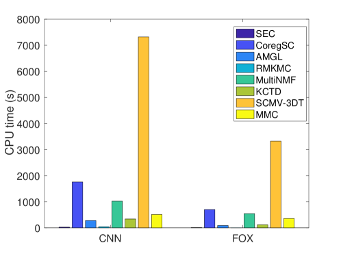
Figure 1: CPU time on large-scale datasets.

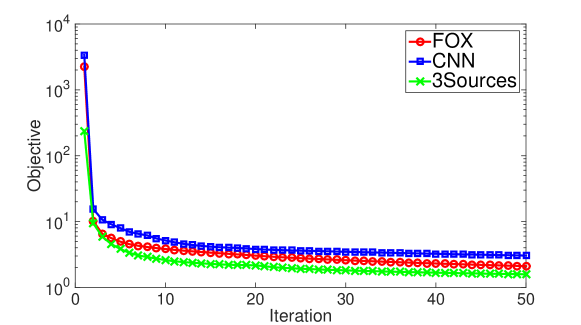
Figure 2: Objective v.s. the number of iterations.

The CPU runtime of comparison methods on large-scale datasets are reported in Figure 1. It is observed that MMC is much faster than CoregSC, MultiNMF and SCMV-3DT. The three methods that are exactly the top-$3$ baseline methods that can almost always perform better than the other baseline methods. Furthermore, the convergence speed of MMC on three datasets is given in Figure 2. It shows that MMC algorithm can converge within few iterations.

V Conclusion

In this paper, we introduced a novel multi-view clustering algorithm MMC based on tensor analysis, which can efficiently learn the underlying latent structure embedded in the full-order feature interactions among multiple views, without the need to construct the higher-order tensor data physically. Experiments on three real-world datasets demonstrate that MMC outperforms several state-of-the-art methods.

References

- [1] G. Chao, S. Sun, and J. Bi, “A survey on multi-view clustering,” arXiv preprint arXiv:1712.06246, 2017.
- [2] L. Sun, Y. Wang, B. Cao, S. Y. Philip, W. Srisa-An, and A. D. Leow, “Sequential keystroke behavioral biometrics for mobile user identification via multi-view deep learning,” in ECML-KDD, 2017, pp. 228–240.
- [3] W. Shao, L. He, C.-T. Lu, X. Wei, and P. S. Yu, “Online unsupervised multi-view feature selection,” in ICDM, 2016.
- [4] A. Kumar, P. Rai, and H. Daume, “Co-regularized multi-view spectral clustering,” in NIPS, 2011, pp. 1413–1421.
- [5] W. Shao, J. Zhang, L. He, and S. Y. Philip, “Multi-source multi-view clustering via discrepancy penalty,” in IJCNN, 2016, pp. 2714–2721.
- [6] F. Nie, J. Li, and X. Li, “Parameter-free auto-weighted multiple graph learning: A framework for multiview clustering and semi-supervised classification,” in IJCAI, 2016.
- [7] C. H. Ding, X. He, and H. D. Simon, “On the equivalence of nonnegative matrix factorization and spectral clustering.” in SDM, 2005, pp. 606–610.
- [8] J. Liu, C. Wang, J. Gao, and J. Han, “Multi-view clustering via joint nonnegative matrix factorization,” in SDM, vol. 13, 2013, pp. 252–260.
- [9] X. Cai, F. Nie, and H. Huang, “Multi-view k-means clustering on big data.” in IJCAI, 2013.
- [10] F. Nie, Z. Zeng, I. W. Tsang, D. Xu, and C. Zhang, “Spectral embedded clustering: A framework for in-sample and out-of-sample spectral clustering,” TNNLS, vol. 22, no. 11, pp. 1796–1808, 2011.
- [11] H. Wang, F. Nie, and H. Huang, “Multi-view clustering and feature learning via structured sparsity,” in ICML, 2013, pp. 352–360.
- [12] M. Yin, J. Gao, S. Xie, and Y. Guo, “Multiview subspace clustering via tensorial t-product representation,” TNNLS, no. 99, pp. 1–14, 2018.
- [13] B. Cao, L. He, X. Wei, M. Xing, P. S. Yu, H. Klumpp, and A. D. Leow, “t-bne: Tensor-based brain network embedding,” in SDM, 2017, pp. 189–197.
- [14] L. Sun, L. He, Z. Huang, B. Cao, C. Xia, X. Wei, and P. S. Yu, “Joint embedding of meta-path and meta-graph for heterogeneous information networks,” in ICBK, 2018.
- [15] B. Cao, L. He, X. Kong, S. Y. Philip, Z. Hao, and A. B. Ragin, “Tensor-based multi-view feature selection with applications to brain diseases,” in ICDM, 2014, pp. 40–49.
- [16] C.-T. Lu, L. He, W. Shao, B. Cao, and P. S. Yu, “Multilinear factorization machines for multi-task multi-view learning,” in WSDM, 2017, pp. 701–709.
- [17] T. G. Kolda and B. W. Bader, “Tensor decompositions and applications,” SIAM review, vol. 51, no. 3, pp. 455–500, 2009.
- [18] F. Nie, H. Huang, X. Cai, and C. H. Ding, “Efficient and robust feature selection via joint -norms minimization,” in NIPS, 2010, pp. 1813–1821.
- [19] W. Shao, L. He, and S. Y. Philip, “Clustering on multi-source incomplete data via tensor modeling and factorization,” in PAKDD, 2015, pp. 485–497.