Identification of Causal Diffusion Effects
Under Structural Stationarity

Abstract

Although social and biomedical scientists have long been interested in the process through which ideas and behaviors diffuse, the identification of causal diffusion effects, also known as peer and contagion effects, remains challenging. Many scholars consider the commonly used assumption of no omitted confounders to be untenable due to contextual confounding and homophily bias. To address this long-standing problem, we examine the causal identification under a new assumption of structural stationarity, which formalizes the underlying diffusion process with a class of dynamic causal directed acyclic graphs. First, we develop a statistical test that can detect a wide range of biases, including the two types mentioned above. We then propose a difference-in-differences style estimator that can directly correct biases under an additional parametric assumption. Leveraging the proposed methods, we study the spatial diffusion of hate crimes against refugees in Germany. After correcting large upward bias in existing studies, we find hate crimes diffuse only to areas that have a high proportion of school dropouts.

Keywords: Contagion effects, Difference-in-differences, Homophily bias, Peer effects, Social influence

1 Introduction

Scientists have long been interested in how ideas and behaviors diffuse across space, networks, and time. For example, social scientists have studied the diffusion of policies and voting behaviors in political science (Sinclair, 2012; Graham et al., 2013; Jones et al., 2017), educational outcomes and crimes in economics (Glaeser et al., 1996; Sacerdote, 2001; Duflo et al., 2011), and innovations and job attainment in sociology (Rogers, 1962; Granovetter, 1973). Epidemiologists and researchers in public health have focused on the spread of infectious disease (Halloran and Struchiner, 1995; Morozova et al., 2018; Cai et al., 2019) and health behavior (Christakis and Fowler, 2013). In each of these research areas, a growing number of scholars aim to estimate the causal impact of diffusion dynamics, that is, how much an outcome of one unit causes, not just correlates with, an outcome of another unit.

Despite its importance, the identification of causal diffusion effects, also known as peer effects, contagion effects, or social influence, is challenging (Manski, 1993; VanderWeele and An, 2013). Although commonly-used statistical methods, including spatial econometric models (e.g., Anselin, 2013), require the assumption of no omitted confounders, this assumption is often untenable due to two well-known types of confounding; contextual confounding and homophily bias (Ogburn, 2018). When there exist some unobserved contextual factors that affect multiple units, we suffer from contextual confounding — we cannot distinguish whether units affect one another through diffusion processes or units are jointly affected by the shared unobserved contextual variables. Homophily bias arises when the spatial or network proximity is affected by some unobserved characteristics. We cannot discern whether units close to one another exhibit similar outcomes because of diffusion or because they selectively become closer in space or networks with others who have similar unobserved characteristics. Emphasizing concerns over these biases, influential papers across disciplines criticize existing diffusion studies (e.g., Cohen-Cole and Fletcher, 2008; Lyons, 2011; Angrist, 2014). In fact, causal diffusion effects are often found to be overestimated by a large amount, for example, by 300 – 700% (Aral et al., 2009; Eckles and Bakshy, 2017). Shalizi and Thomas (2011) argue that it is nearly impossible to credibly estimate causal diffusion effects from observational studies by relying on the conventional assumption of no omitted confounders.

To address this long-standing challenge, we examine the identification of causal diffusion effects under a new assumption of structural stationarity, which formalizes diffusion processes with a causal directed acyclic graph (DAG) approach (Pearl, 2000; Ogburn and VanderWeele, 2014). In particular, we assume that the underlying causal DAG belongs to a class of dynamic causal DAGs (Dean and Kanazawa, 1989; Pearl and Russell, 2001), which repeat nonparametric causal substructure over time (Section 4.1). Thus, the structural stationarity assumption requires the existence of causal relationships among variables — not the effect or sign of such relationships — to be stable over time. This is in contrast to a usual DAG-based approach that assumes a specific causal DAG and the full knowledge of its structure, which may be difficult to justify in applied contexts. Instead, we propose methodologies that have the same statistical guarantees for any causal DAG within the general class of dynamic causal DAGs.

Under the structural stationarity, we first develop a placebo test that uses a lagged dependent variable to detect a wide class of biases, including contextual confounding and homophily bias (Section 4.2). It assesses whether a lagged dependent variable is conditionally independent of the treatment variable. We prove statistical properties of the test based on a new theorem, which states that under the structural stationarity, the no omitted confounders assumption is equivalent to the conditional independence of a lagged dependent variable and the treatment variable. This proof exploits the structure of back-door paths (Pearl, 1995) and the graphical representation of the no omitted confounders assumption (Shpitser, VanderWeele, and Robins, 2012) under the structural stationarity.

In addition, we propose a bias-corrected estimator that can directly remove biases under an additional parametric assumption (Section 4.3). In its basic form, it subtracts the bias detected by the placebo test from a biased estimator. We prove unbiasedness of this estimator under a parametric assumption that the effect and imbalance of unobserved confounders are constant over time. We describe its connection to the widely-used difference-in-differences estimator (Angrist and Pischke, 2008; Sofer et al., 2016).

Applying the proposed methods, we study the spatial diffusion of hate crimes against refugees in Germany. Facing the biggest refugee crisis since the Second World War, Germany has recently registered more than 1 million asylum applications, making them the largest refugee-hosting country in Europe (United Nations High Commissioner for Refugees., 2017). During this time period, the number of hate crimes against refugees has substantially increased, a close to 200% increase from 2015 to 2016. A clear, descriptive pattern is that the incidence of hate crimes was spatially clustered and the number grew over time as waves (see Section 2). However, what is the causal process behind this dynamic spatial pattern? Understanding the causal impact of hate crime diffusion is of policy and scientific interest to prevent further spread of hate crimes. We leverage the proposed placebo test and bias-corrected estimator to tackle concerns about unmeasured contextual confounding. See Section 2 for the details of the data and Section 5 for empirical analysis.

This article builds on a growing literature of causal diffusion effects (Shalizi and Thomas, 2011; Goldsmith-Pinkham and Imbens, 2013; Ogburn, 2018). In addition to research on the use of experimental or quasi-experimental design (Bramoullé et al., 2009; O’Malley et al., 2014; An, 2015; Taylor and Eckles, 2017; Basse et al., 2019; Jagadeesan et al., 2019; Li et al., 2019), a series of papers address problems of omitted confounders by deriving tests or bounds (e.g., Anagnostopoulos et al., 2008). VanderWeele et al. (2012) show that after controlling for homophily bias and contextual confounding, the spatial autoregressive model can be used to test the existence of diffusion effects. To compute bounds for diffusion effects, Ver Steeg and Galstyan (2010, 2013) examine a specific causal DAG only with homophily and diffusion, and VanderWeele (2011) proposes sensitivity analysis methods. This paper shares concerns about the no omitted confounders assumption. However, instead of testing the existence of diffusion effects or deriving bounds, this paper focuses on the point identification and estimating the magnitude of causal diffusion effects.

This paper also draws upon emerging literature of negative controls (Lipsitch et al., 2010; Tchetgen Tchetgen, 2013). In particular, this paper extends recent studies using negative controls in panel data settings (Sofer et al., 2016; Flanders et al., 2017; Miao and Tchetgen Tchetgen, 2017) to the identification of causal diffusion effects. The proposed methods differ from the previous literature in that we use the structural stationarity, which assumes a class of dynamic causal DAGs rather than one specific causal DAG. This class of dynamic causal DAGs (Pearl and Russell, 2001) is a causal extension of the dynamic bayesian networks (DBN) popular in the probabilistic graphical modeling literature (e.g., Murphy, 2002). The key difference is that while the DBN often assumes the parameters of conditional probability distributions are time-invariant, the dynamic causal DAG only assumes the stability of the nonparametric causal structure and allows for any higher-order Markov model. Finally, causal DAGs (Pearl, 2000) are useful not only for causal identification but also for asymptotic statistical inference. van der Laan (2014) and Ogburn et al. (2017) offer one of the first foundations to use causal directed acyclic graphs for network data. Tchetgen Tchetgen et al. (2017) provide an alternative approach using chain graphs. Because we focus on the identification of causal diffusion effects, our proposed methods are complementary to these recent papers that develop theories of statistical inference in a network asymptotic regime.

2 A Motivating Empirical Application:
Spatial Diffusion of Hate Crimes against Refugees

Research across the social sciences has shown that many types of violence are contagious (Wilson and Kelling, 1982; Myers, 2000). One small act of violence can trigger another act of violence, which again induces another, and can lead to waves of violence (Hill and Rothchild, 1986; Buhaug and Gleditsch, 2008). Without taking into account how violent behaviors spread across space, it is difficult to explain when, where, and why some areas experience violence and to prevent further spread of violence.

In this paper, we investigate the spatial diffusion of hate crimes against refugees in Germany, one of the most pressing problems in the country. Over the last few years, Germany has experienced a record influx of refugees (Bundesamt für Migration und Flüchtlinge, 2019), and during the same time period, the number of hate crimes against refugees has increased substantially. Our primary data source of hate crimes is a project, Mut gegen rechte Gewalt (courage against right-wing violence), by the Amadeu Antonio Foundation and the weekly magazine Stern, which has been documenting anti-refugee violence in Germany since the beginning of 2014. This data source has been recently analyzed by several papers (e.g., Benček and Strasheim, 2016; Jäckle and König, 2016). The dataset we analyze in this paper is compiled by Dancygier et al. (2019), who extended this hate crime data by merging in other variables, such as the number of refugees, the population size, a proportion of school dropouts and unemployment rates, collected from the Federal Statistical Office in Germany.

Figure 1 (a) reports the number of physical attacks against refugees each month, from the beginning of 2015 to the end of 2016. While there were about 15 hate crimes on average in each month of 2015, this rose to more than 40 in 2016, a close to 200% increase. Figure 1 (b) presents the spatial patterns over the two years. Two empirical patterns are worth noting. First, hate crimes were spatially clustered in East Germany. Second, the number of counties that experience hate crimes grew over time as waves. This dynamic spatial pattern is consistent with the spatial diffusion theory which argues that hate crimes diffuse from one county to another spatially proximate county over time (Myers, 2000; Braun, 2011). Indeed, Jäckle and König (2016) found that the incidence of hate crimes in one county predicts that of hate crimes in its spatially proximate counties using the data from Germany in 2015.

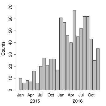
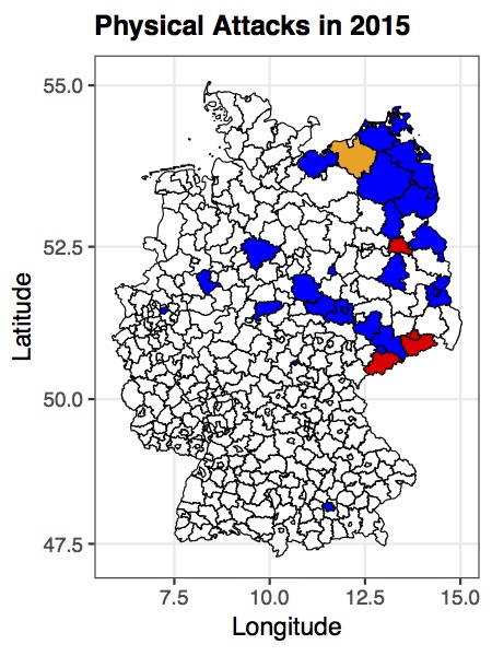
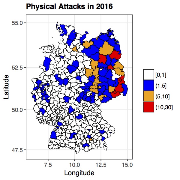
(a) Time Trend                                           (b) Spatial Patterns

Figure 1: Temporal and Spatial Patterns of Hate Crimes in Germany. Note: The left figure shows the number of physical attacks each month. In the middle and right figures, we show the number of physical attacks in each county in 2015 and 2016, respectively. Each of 402 counties is colored in white, blue, orange, or red if the number of hate crimes in a given year is less than or equal to 1, 5, 10, or greater than 10, respectively.

However, it is challenging to estimate the causal impact of this spatial diffusion process because there exist well-known concerns of contextual confounding: many unobserved confounders can be spatially correlated. For example, the number of refugees increased substantially during this period and is also spatially correlated. Even if we collect a long list of covariates, it is difficult to assess whether a selected set of control variables is sufficient for removing contextual confounding. To address this type of pervasive concerns over bias, we develop a placebo test to detect bias and a bias-corrected estimator to remove bias. The main empirical analysis appears in Section 5. Although our empirical application focuses on the spatial diffusion problem, the proposed approach is also applicable to network diffusion settings where homophily bias is a common concern.

3 The Setup for Causal Diffusion Analysis

Causal diffusion, also known as peer and contagion effects, refers to a process in which an outcome of one unit influences an outcome of another unit over time (Shalizi and Thomas, 2011; VanderWeele et al., 2012). This section introduces the setup for analyzing such causal diffusion. We define the average causal diffusion effect and then describe challenges for its identification.

3.1 Average Causal Diffusion Effect

Consider $n$ units over $T$ time periods. Let $Y_{it}$ be the outcome for unit $i$ at time $t$ for $i\in\{1,\ldots,n\}$ and $t\in\{0,1,\ldots,T\}.$ Use $\mathbf{Y}_{t}$ to denote a vector $(Y_{1t},\ldots,Y_{nt})$, which contains the outcomes at time $t$ for $n$ units. To encode spatial or network connections between these $n$ units, we follow the standard spatial statistics literature (Cressie, 2015) and use a distance matrix $\mathbf{W}$ where $\mathbf{W}$ can be an asymmetric, weighted matrix. In the motivating application, it is of interest to estimate how much hate crimes in one county diffuse to other spatially proximate counties. Here, the distance matrix $\mathbf{W}$ could encode physical distance between counties where $W_{ij}$ might be an inverse of the distance between district $i$ and $j$. In network diffusion settings, $W_{ij}$ could represent a directed tie, e.g., whether unit $i$ follows unit $j$ in a Twitter network. Define neighbors $\mathcal{N}_{i}$ to be other units who are connected with a given unit $i$, i.e., $\mathcal{N}_{i}\equiv\{j:W_{ij}\neq 0\}.$ In spatial diffusion analysis, researchers often assign $0$ to $W_{ij}$ when the distance between two units is greater than a certain threshold, e.g., 100 km.

We rely on potential outcomes (Neyman, 1923; Rubin, 1974) to formally define causal diffusion effects. Based on the tradition of spatial econometrics (Anselin, 2013; Franzese and Hays, 2007), this paper focuses on the weighted average of the neighbors’ outcomes $\mathbf{W}_{i}^{\top}\mathbf{Y}_{t}$ as the treatment variable. Although we keep this setup throughout the paper, the methods in this paper can be easily applied to other definitions of the treatment variable. We use $D_{it}\equiv\mathbf{W}_{i}^{\top}\mathbf{Y}_{t}$ to denote the treatment variable and let $Y_{i,t+1}(d)$ represent the potential outcome variable of unit $i$ at time $t+1$ if the unit receives the treatment $D_{it}=d$.

We are interested in the average causal diffusion effect (ACDE) at time $t+1$, which is defined as the average causal effect of the treatment variable $D_{it}$ on the outcome at time $t+1$ (Ogburn and VanderWeele, 2014; Ogburn, 2018). It is the comparison between the potential outcome under a higher value of the treatment $D_{it}=d^{H}$ and the potential outcome under a lower value of the treatment $D_{it}=d^{L}.$

Definition 1 (Average Causal Diffusion Effect).

The average causal diffusion effect (ACDE) at time $t+1$ is defined as,

$$\tau_{t+1}(d^{H},d^{L})\equiv\mathbb{E}[Y_{i,t+1}(d^{H})-Y_{i,t+1}(d^{L})],$$ (1)

where $d^{H}$ and $d^{L}$ are two constants specified by researchers.

For example, the ACDE could quantify how much the risk of having hate crimes in the next month changes if we see more hate crimes in neighboring counties this month. This captures how much hate crimes diffuse across space over time.

Finally, we introduce an assumption about the measurement of outcomes. We assume that we observe one of the potential outcomes at every time period $t=1,\ldots,T$.

Assumption 1 (Sequential Consistency).

For every unit at every time period $t=1,\ldots,T$, one of the potential outcome variables is observed, and the realized outcome variable for unit $i$ at time $t+1$ is denoted by

$$Y_{i,t+1}=Y_{i,t+1}(D_{it}).$$ (2)

This is a simple extension of the consistency assumption widely used in the cross-sectional settings (VanderWeele, 2009) to the diffusion setup. The assumption means that we avoid the temporal aggregation problem (Granger, 1988) that can mask the dynamics of the underlying diffusion process. Its violation implies simultaneity bias, that is, the treatment variable and the outcome variable simultaneously cause each other (Danks and Plis, 2013; Hyttinen et al., 2016). In the literature of causal diffusion analysis, this assumption is essential because, without it, the causal order of the treatment and outcome becomes ambiguous, and causal diffusion effects are no longer well-defined (Lyons, 2011; Ogburn and VanderWeele, 2014; Ogburn, 2018). See Zhang et al. (2011) for a similar problem in the structural nested model and g-estimation. In practice, researchers can make this assumption more plausible by measuring outcomes frequently. For example, the assumption could be more tenable when we can measure the incidence of hate crimes monthly rather than annually. We maintain this assumption throughout the paper given its essential role in defining the ACDE, but in Appendix A.3, we also discuss the connection between its violation and the proposed placebo test.

3.2 Identification under No Omitted Confounders Assumption

We now describe the widely used identification assumption of no omitted confounders and explain pervasive concerns about its violation. This assumption states that all relevant confounders are in a selected set of control variables. Formally, the potential outcomes at time $t+1$ are independent of a joint distribution of neighbors’ outcomes at time $t$ given control variables.

Assumption 2 (No Omitted Confounders).

For $i=1,2,\ldots,n$,

$$Y_{i,t+1}(d)\ \mbox{$\perp\!\!\!\perp$}\ \{Y_{jt}\}_{j\in\mathcal{N}_{i}}\ \mid\mathbf{C}_{i,t+1},$$ (3)

for $d\in\mathcal{D}$ where $\mathcal{D}$ is the support of $D_{it}$, and $\mathbf{C}_{i,t+1}$ is a set of pretreatment variables, which we call a control set. Note that control set $\mathbf{C}_{i,t+1}$ can include time-independent variables and time-dependent variables measured at time $t+1$ or before $t+1$.

Under the assumption of no omitted confounders, the ACDE is identified as follows.

$$\tau_{t+1}(d^{H},d^{L})=\int_{\mathcal{C}}\biggl{\{}\mathbb{E}[Y_{i,t+1}|D_{it}=d^{H},\mathbf{C}_{i,t+1}=\mathbf{c}]-\mathbb{E}[Y_{i,t+1}|D_{it}=d^{L},\mathbf{C}_{i,t+1}=\mathbf{c}]\biggr{\}}dF_{\mathbf{C}_{i,t+1}}(\mathbf{c}),$$ (4)

where $F_{\mathbf{C}_{i,t+1}}(\mathbf{c})$ is the cumulative distribution function of $\mathbf{C}_{i,t+1}$ and the standard overlap assumption is made: $\Pr(D_{it}=d^{H}|\mathbf{C}_{i,t+1}=\mathbf{c})>0$ and $\Pr(D_{it}=d^{L}|\mathbf{C}_{i,t+1}=\mathbf{c})>0$ for $i=1,\ldots,n$ and all $\mathbf{c}\in\mathcal{C}$ where $\mathcal{C}$ is the support of $\mathbf{C}_{i,t+1}$. We can estimate the ACDE by estimating the conditional expectation $\mathbb{E}[Y_{i,t+1}|D_{it},\mathbf{C}_{i,t+1}]$ and then averaging it over the empirical distribution of control variables $\mathbf{C}_{i,t+1}$.

Although many empirical studies of diffusion make the assumption of no omitted confounders, it is widely known that the assumption is often questionable in practice (Manski, 1993; Shalizi and Thomas, 2011; VanderWeele and An, 2013). This concern is pervasive mainly because it implies the absence of two well-known types of biases: contextual confounding and homophily bias. Contextual confounding – the primary focus of the spatial diffusion literature – can exist when units share some unobserved contextual factors. For example, in the motivating application of hate crime diffusion, the risk of having hate crimes is likely to be affected by some economic policies, which often affect multiple counties at the same time. In this case, researchers might observe spatial clusters of hate crimes even without diffusion. Another well-known type of bias is homophily bias – the main concern in the network diffusion literature. This bias arises when units become connected due to their unobserved characteristics. For example, voters who are connected to each other can have similar political opinions without any diffusion or social influence because people who have similar political views might become friends in the first place (Fowler et al., 2011). We discuss the causal DAG representation of these biases when we introduce our proposed methods in Section 4.

4 The Proposed Methodology

In this section, we examine the identification of causal diffusion effects under a new assumption of structural stationarity. After introducing the assumption (Section 4.1), we first develop a statistical placebo test to detect a wide range of biases (Section 4.2) and then propose a bias-corrected estimator (Section 4.3).

4.1 Structural Stationarity

We formalize the underlying diffusion process with a causal directed acyclic graph (DAG) framework (Pearl, 2000). In particular, we assume the structural stationarity, which states the underlying causal DAG belongs to a general class of dynamic causal DAGs (Dean and Kanazawa, 1989; Pearl and Russell, 2001). It requires that the existence of causal relationships between variables, not the effect or sign of such relationships, to be stable over time. A class of dynamic causal DAGs and the structural stationarity are formally defined as follows. We review basic causal DAG terminologies in Appendix B.

Definition 2 (Dynamic Causal DAGs (Dean and Kanazawa, 1989; Pearl, 2000)).

Consider variables in a causal DAG $\mathcal{G}$ that have more than one child or have at least one parent. Among these variables, distinguish two types; the time-independent variable $Z_{i}$ and the time-dependent variable $X_{it}$. A class of dynamic causal DAGs is any causal DAG $\mathcal{G}$ that satisfies the following conditions.

$$(2.1)\ \ X_{it}\in\mbox{PA}(X_{i,t+1})\ \ \mbox{ for }i\in\{1,\ldots,n\}\mbox{ and }\ t=0,\ldots,T-1.$$

$$(2.2)\ \ \mbox{For}\ i,i^{\prime}\in\{1,\ldots,n\},\ \exists\ t,k\ \mbox{s.t. }X_{it}\in\mbox{PA}(\widetilde{X}_{i^{\prime},t+k})\Rightarrow\ X_{it^{\prime}}\in\mbox{PA}(\widetilde{X}_{i^{\prime},t^{\prime}+k})\ \mbox{ for all }t^{\prime}=0,\ldots,T-k.$$

$$(2.3)\ \ \mbox{For}\ i,i^{\prime}\in\{1,\ldots,n\},\ \exists\ t\ \mbox{s.t. }Z_{i}\in\mbox{PA}(X_{i^{\prime}t})\ \Rightarrow\ Z_{i}\in\mbox{PA}(X_{i^{\prime}t^{\prime}})\ \mbox{ for all }t^{\prime}=0,\ldots,T,$$

where $A\in\mbox{PA}(B)$ indicates that variable $A$ is a parent of variable $B$.

Assumption 3 (Structural Stationarity).

The distribution over outcome $Y$, treatment $D$, and control variables $\mathbf{C}$ is faithful to one of the dynamic causal DAGs.

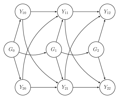
(a) Structural Stationarity         (b) Violation of Structural Stationarity

Figure 2: Illustration of Structural Stationarity. Note: Six nodes $Y_{it}$ represent outcome variables for two individuals $i\in\{1,2\}$ over three time periods $t\in\{0,1,2\}.$ Three nodes $G_{t}$ are contextual variables for $t\in\{0,1,2\}.$ In the first panel, the causal structure between variables $Y$ and $G$ are stable over time. In the second panel, variable $G$ has no effect on $Y$ at $t=2$ and thus the structural stationarity is violated.

The faithfulness is defined as follows. If a distribution is faithful to causal directed acyclic graph $\mathcal{G}$, variables $A$ and $B$ are independent if and only if the variables are d-separated in $\mathcal{G}$ (Spirtes et al., 2000). Condition 2.1 of Definition 2 requires that all time-dependent variables that have at least one parent be affected by their own lagged variables. This condition is more plausible when the time intervals are shorter. Condition 2.2 means that if two time-dependent variables have a child-parent relationship at one time period, the same causal relationship should exist for all other time periods. Similarly, Condition 2.3 requires that if a time-independent variable is a parent of a time-dependent variable at one time period, the same child-parent relationship should exist at all other time periods. The last two requirements are the core – the existence of causal relationships should be stable over time. Importantly, the effect of each variable can be changing over time; the only requirement is the time-invariant existence of the causal relationships. Figure 2 visualizes examples of the structural stationarity and its violation.

In our motivating application, suppose that the unemployment rate is a confounder in one month. Then, the structural stationarity requires that the unemployment rate should remain a confounder during the time periods we analyze. The assumption is violated when a set of confounders changes over time. The effect of the unemployment rate can be changing over time.

Several points are worth noting. First, the structural stationarity only assumes a class of dynamic causal DAGs rather than a specific dynamic causal DAG. This is in contrast to conventional DAG approaches that assume one particular DAG and require full knowledge of its DAG structure. Thus, researchers can rely on the structural stationarity assumption even when they cannot justify their full knowledge of the underlying DAG structure, as far as the existence of causal relationships is time-invariant.

Second, the structural stationarity is often a natural requirement in applied contexts. In fact, causal DAGs in several important papers about causal diffusion effects (Shalizi and Thomas, 2011; O’Malley et al., 2014; Ogburn and VanderWeele, 2014) are examples of dynamic causal DAGs. Causal DAGs in the causal discovery literature often impose a similar but stronger condition (Danks and Plis, 2013; Hyttinen et al., 2016). They often assume that variables are affected only by one-time lag (also known as the first-order Markov assumption) and this structure is time-invariant. In contrast, the structural stationarity allows for any higher-order temporal dependence (see Condition 2.2 of Definition 2). Finally, when the underlying causal structure changes at some time, the structural stationarity is violated. However, if researchers know the time when the underlying structure changes, we can still make use of the structural stationarity assumption separately, before and after this time point.

4.2 Placebo Test to Detect Bias

Under the structural stationarity, we propose a placebo test – using a lagged dependent variable as a general placebo outcome – that can detect a wide class of biases, including contextual confounding and homophily bias. This placebo test helps the credible identification of causal diffusion effects by statistically assessing the validity of the confounder adjustment. We focus on theories and methodologies of the placebo test in this section, and we provide a simulation study calibrated to the hate crime data in Appendix C.1.

4.2.1 Equivalence Theorem

The proposed placebo test exploits a lagged dependent variable as a placebo outcome. It tests the assumption of no omitted confounders by assessing whether a lagged dependent variable is conditionally independent of the treatment variable. This placebo test is formally justified based on the equivalence theorem, which states that, under the structural stationarity, the assumption of no omitted confounders is equivalent to the conditional independence of the simultaneous outcomes given a placebo set defined below. This theorem and the placebo test are formally written as follows.

Theorem 1 (Equivalence between No Omitted Confounders Assumption and Conditional Independence of Simultaneous Outcomes).

Under Assumption 1 and Assumption 3,

$$Y_{i,t+1}(d)\ \mbox{$\perp\!\!\!\perp$}\ \{Y_{jt}\}_{j\in\mathcal{N}_{i}}\mid\mathbf{C}_{i,t+1}\ \Longleftrightarrow Y_{it}\ \mbox{$\perp\!\!\!\perp$}\ \{Y_{jt}\}_{j\in\mathcal{N}_{i}}\mid\mathbf{C}_{i,t+1}^{P},$$ (5)

where a placebo set $\mathbf{C}^{P}$ is defined as

$$\mathbf{C}_{i,t+1}^{P}\equiv\{\mathbf{C}_{i,t+1},\mathbf{C}_{i,t+1}^{(-1)},\{Y_{j,t-1}\}_{j\in\mathcal{N}_{i}}\}\setminus\mbox{Des}(Y_{it}),$$ (6)

where $\mathbf{C}_{i,t+1}^{(-1)}$ is a lag of the time-dependent variables in $\mathbf{C}_{i,t+1}$, $\{Y_{j,t-1}\}_{j\in\mathcal{N}_{i}}$ is a lag of the treatment variable, and $\mbox{Des}(Y_{it})$ is a descendant of $Y_{it}$, i.e., variables affected by $Y_{it}$. As a regularity condition, we assume that the violation of the no omitted confounders assumption, if any, is due to unobserved confounders, i.e., the change in the lag-structure of the selected control set cannot remove the bias (see Appendix A.1 for details).

Placebo Test: For a given control set $\mathbf{C}$, the following test statistically assesses whether the control set contains all confounders, i.e., Assumption 2.

1. Step 1: Derive placebo set $\mathbf{C}_{i,t+1}^{P}$ from control set $\mathbf{C}_{i,t+1}$ based on equation (6).

2. Step 2: Test the conditional independence, $Y_{it}\ \mbox{$\perp\!\!\!\perp$}\ \{Y_{jt}\}_{j\in\mathcal{N}_{i}}\mid\mathbf{C}_{i,t+1}^{P}.$

Note: the first step follows a deterministic rule to derive placebo set $\mathbf{C}_{i,t+1}^{P}$.
(1) add lags of existing control variables and a lag of the treatment variable to the original control set $\mathbf{C}$, and (2) remove all the variables affected by outcomes at time $t$.

The proof of Theorem 1 (in Appendix A.1) exploits the structure of back-door paths (Pearl, 1995) and the graphical representation of the no omitted confounders assumption (Shpitser, VanderWeele, and Robins, 2012) under the structural stationarity. In equation (5), the assumption of no omitted confounders (the left-hand side) is proven to be equivalent to the conditional independence of the observed outcome of individual $i$ and her neighbors’ outcomes at the same time period given a placebo set (the right-hand side). Because this right-hand side is observable and testable, this theorem directly implies that we can statistically assess the assumption of no omitted confounders by the placebo test of the conditional independence of the simultaneous outcomes $Y_{it}\ \mbox{$\perp\!\!\!\perp$}\ \{Y_{jt}\}_{j\in\mathcal{N}_{i}}\mid\mathbf{C}_{i,t+1}^{P}$.

The basic idea behind the theorem is as follows: under the structural stationarity, back-door paths between the main outcome and the treatment are similar to those between the lagged dependent variable and the treatment. The difference between control set $\mathbf{C}$ and placebo set $\mathbf{C}^{P}$ is to formally guarantee that unblocked back-door paths between the main outcome and the treatment are the same (from a causal graph perspective) to those between the placebo outcome and the treatment. To derive this placebo set, we only need to know which variables in the control set are time-dependent and which variables are affected by outcomes at time $t$. The former information is often readily available, and the latter one is the same as the information used to avoid post-treatment bias in the standard causal inference settings.

(a) Example of Placebo Test

Figure 3: Illustration of Placebo Test. Note: We focus on the ACDE of $Y_{11}$ on $Y_{22}$ where $Y_{11}$ is the treatment variable (blue), $Y_{22}$ is the outcome variable (red), and the causal arrow of interest $Y_{11}\rightarrow Y_{22}$ is colored blue. The placebo outcome $Y_{21}$ is colored orange.

4.2.2 Illustrations with Causal DAGs

Although the proposed placebo test is applicable to any causal DAGs that satisfy the structural stationarity, we consider a causal DAG in Figure 4.2.1 (a) as one concrete example. The causal DAG has twelve nodes in total; six nodes $Y_{it}$ representing outcome variables for two individuals $i\in\{1,2\}$ over three time periods $t\in\{0,1,2\},$ three nodes $G_{t}$ representing contextual variables for $t\in\{0,1,2\},$ two nodes $U_{i}$ representing individual-level characteristics for $i\in\{1,2\},$ and finally variable $W$ indicating the connection of two individuals, taking $1$ if they are connected and $0$ otherwise. Suppose we are interested in the ACDE of $Y_{11}$ on $Y_{22}$ where $Y_{11}$ is the treatment variable (blue), $Y_{22}$ is the outcome variable (red), and the causal arrow of interest $Y_{11}\rightarrow Y_{22}$ is colored blue. The placebo outcome $Y_{21}$ is colored orange.

Based on this causal DAG in Figure 4.2.1 (a), Table in Figure 4.2.1 (b) shows four different scenarios: no bias, contextual confounding, homophily bias, and both types of biases. For each set of control variables, the placebo test checks conditional independence, $Y_{11}\ \mbox{$\perp\!\!\!\perp$}\ Y_{21}\mid\mathbf{C}^{P}$ where we derive a placebo set $\mathbf{C}^{P}$ from a chosen control set $\mathbf{C}$ using equation (6). These scenarios show how the placebo test detects biases by exploiting the structural stationarity.

First, when we control for three variables $\{Y_{21},U_{2},G_{2}\},$ the ACDE of interest is identified (“No Bias”). Without knowledge of the entire causal DAG, we can assess the absence of bias by implementing the placebo test. Following equation (6), we derive a placebo set $\mathbf{C}^{P}=\{Y_{20},Y_{10},U_{2},G_{2},G_{1}\}$ and then the placebo test checks $Y_{11}\mbox{$\perp\!\!\!\perp$}Y_{21}|\mathbf{C}^{P}.$ In Figure 4.2.1 (a), there is no unblocked back-door path between $Y_{11}$ and $Y_{21}$, and the conditional independence holds as Theorem 1 implies.

Second, we consider a typical form of contextual confounding. When we control for two variables $\{Y_{21},U_{2}\},$ the ACDE is not identified due to a back-door path ($Y_{11}\leftarrow G_{1}\rightarrow G_{2}\rightarrow Y_{22}$). We now verify that the placebo test correctly detects this bias. We first derive a placebo set as $\mathbf{C}^{P}=\{Y_{20},Y_{10},U_{2}\}$ and then assess whether there is any unblocked back-door path between $Y_{11}$ and $Y_{21}.$ In fact, we correctly reject the placebo test; $Y_{11}\centernot{\mbox{$\perp\!\!\!\perp$}}Y_{21}|\mathbf{C}^{P}$ due to a back-door path $(Y_{11}\leftarrow G_{1}\rightarrow Y_{21})$.

Finally, we investigate homophily bias. When we control for three variables $\{Y_{21},G_{2},G_{1}\},$ the ACDE is not identified due to a back-door path ($Y_{11}\leftarrow U_{1}\rightarrow\framebox{$W$}\leftarrow U_{2}\rightarrow Y_{22}$) where the square box means that connection variable $W$ is adjusted for. As shown in Shalizi and Thomas (2011), $W$ is always, often implicitly, adjusted for in any causal diffusion analysis because researchers need to compare observations with similar spatial/network pre-treatment characteristics. In this case, a placebo set is $\mathbf{C}^{P}=\{Y_{20},Y_{10},G_{2},G_{1},G_{0}\}$ and we can verify that $Y_{11}\centernot{\mbox{$\perp\!\!\!\perp$}}Y_{21}|\mathbf{C}^{P}$ due to a back-door path ($Y_{11}\leftarrow U_{1}\rightarrow\framebox{$W$}\leftarrow U_{2}\rightarrow Y_{21}$). The placebo test correctly detects homophily bias. If we follow the same logic, it is straightforward to verify that the placebo test can also detect biases even when contextual confounding and homophily bias coexist.

4.2.3 Connection to Spatial Autoregressive Model

Although there are many ways to implement the second step of the placebo test, one approach is a parametric test based on the spatial autoregressive (SAR) model (e.g., Anselin, 2013; Cressie, 2015). For example, when outcomes are continuous, we can implement the placebo test by the following linear spatial autoregressive model.

$$Y_{it} = \alpha_{0}+\delta\mathbf{W}_{i}^{\top}\mathbf{Y}_{t}+\gamma_{0}^{\top}\mathbf{C}_{i,t+1}^{P}+\epsilon_{it},$$ (7)

where $\mathbf{W}_{i}^{\top}\mathbf{Y}_{t}\equiv D_{it}$ is the treatment variable, $\mathbf{C}_{i,t+1}^{P}$ is a placebo set, and $\epsilon_{it}$ is an error term. In the motivating application (Section 5), we employ logistic spatial autoregressive model in a similar way. It is important to note that the equivalence theorem (Theorem 1) is nonparametric, so researchers can combine the theorem with any nonparametric or parametric models in applied settings.

Theorem 1 implies that the placebo outcome $Y_{it}$ is conditionally independent of the treatment variable when the assumption of no omitted confounders (Assumption 2) holds. Therefore, the spatial autoregressive coefficient $\delta$ serves as a test statistic of the placebo test. By testing whether this spatial autoregressive coefficient is zero, researchers can assess the no omitted confounders assumption and thus detect biases, including contextual confounding and homophily bias. In Appendix C.1, we investigate the statistical power of the proposed placebo test through simulation studies and show that its power is comparable to a theoretical upper bound.

This use of the SAR model as a placebo test differs from existing approaches in the spatial econometrics literature that are designed to capture spatial correlations (e.g., Anselin, 2013). While researchers conventionally interpret the spatial autoregressive coefficient as the strength of the spatial correlation, the proposed placebo test uses the spatial autoregressive coefficient to detect biases rather than to estimate diffusion effects. For the estimation of the ACDE, we estimate the conditional expectation $\widehat{\mathbb{E}}[Y_{i,t+1}\mid D_{it},\mathbf{C}_{i,t+1}]$ and then uses the identification formula in equation (4).

It is important to note that if the parametric assumptions of the model are violated, the spatial autoregressive coefficient in equation (7) can be zero even when unmeasured confounding remains. Like any other statistical tests, a specific parametric placebo test can fail if its underlying parametric assumptions do not hold. A key advantage of the proposed approach is that the equivalence theorem (Theorem 1) is nonparametric. The theorem implies that when there exist no omitted confounders, the placebo outcome and the treatment are conditionally independent in any parametric and nonparametric tests. Therefore, in practice, researchers can verify the conditional independence of the placebo outcome and the treatment variable using additional non- or semiparametric conditional independence tests (e.g., Su and White, 2008; Zhang et al., 2012).

4.3 Bias-Corrected Estimator

If the placebo test detects bias, one may want to collect more data and improve the selection of control variables. This strategy might, however, be infeasible in many applied settings. To help researchers in such common situations, this section considers how to correct biases by introducing an additional parametric assumption. We start with a simple example of linear models (Section 4.3.1) and then provide general results in Sections 4.3.2 and 4.3.3. We provide simulation evidence in Appendix C.2.

4.3.1 An Example with Linear Models

To develop an intuition for a bias-corrected estimator, we first consider a simple example with linear models. We assume here that a selected set of control variables is time-independent and the same as its corresponding placebo set. A general result is provided in the following subsections.

Suppose we fit a linear model in which we regress the outcome at time $t+1$ on the treatment variable and the selected control set.

$$Y_{i,t+1} = \alpha+\beta D_{it}+\gamma^{\top}\mathbf{C}_{i,t+1}+\tilde{\epsilon}_{i,t+1},\vspace{-0.1in}$$ (8)

where $D_{it}$ is the treatment variable, $\mathbf{C}_{i,t+1}$ is the selected control set, and $\tilde{\epsilon}_{i,t+1}$ is an error term. If the assumption of no omitted confounders (Assumption 2) holds, $\hat{\beta}\times(d^{H}-d^{L})$ is an unbiased estimator of the ACDE given that the linear model specification is correct. In contrast, when the no omitted confounders assumption is violated, this estimator is biased. We would like to assess whether the assumption of no omitted confounders holds and also correct biases, if any.

To assess the assumption of no omitted confounders, suppose we run a parametric placebo test using the following linear spatial autoregressive model as in equation (7).

$$Y_{it} = \alpha_{0}+\delta D_{it}+\gamma_{0}^{\top}\mathbf{C}_{i,t+1}^{P}+\epsilon_{it},\vspace{-0.1in}$$

where $\mathbf{C}_{i,t+1}^{P}$ is a placebo set and $\epsilon_{it}$ is an error term. If the assumption of no omitted confounders holds, the spatial autoregressive coefficient $\delta$ should be zero (Theorem 1). In contrast, if the assumption of no omitted confounders does not hold, an estimated coefficient $\hat{\delta}$ then serves as a bias-correction term.

In this simple example, a proposed bias-corrected estimator is given by subtracting the bias-correction term $\hat{\delta}$ from an original biased estimator $\hat{\beta}$.

$$\hat{\tau}_{BC}(d^{H},d^{L})\ \equiv\ (\hat{\beta}-\hat{\delta})\times(d^{H}-d^{L}).\vspace{-0.1in}$$ (9)

This bias-corrected estimator is unbiased for the ACDE for the treated under an additional parametric assumption we discuss in detail in the next subsection (Assumption 4). Note that when the assumption of no omitted confounders holds, the expected value of $\hat{\delta}$ is zero, meaning no bias correction.

4.3.2 Assumption

To describe a general bias-corrected estimator, we begin by defining the average causal diffusion effect for the treated (ACDT). We will show in Theorem 2 that the proposed bias-corrected estimator is unbiased for the ACDT. The formal definition is as follows.

$$\tau^{d^{H}}_{t+1}(d^{H},d^{L})\equiv\mathbb{E}[Y_{i,t+1}(d^{H})-Y_{i,t+1}(d^{L})\mid D_{it}=d^{H}].$$ (10)

This is the average causal diffusion effect for units who received the higher level of the treatment. This quantity could represent the causal diffusion effect of hate crimes for counties in a higher risk neighborhood, i.e., $d^{H}\%$ of neighboring counties had hate crimes in month $t$.

To introduce necessary assumptions, we divide a control set into three types of variables $\mathbf{C}_{i,t+1}\ \equiv\ \{\mathbf{X}_{i,t+1},\mathbf{V}_{i,t+1},\mathbf{Z}_{i}\}$ where (1) $\mathbf{X}_{i,t+1}$, the time-dependent variables that are descendants of $Y_{it}$, (2) $\mathbf{V}_{i,t+1}$, the time-dependent variables that are not descendants of $Y_{it}$, and (3) $\mathbf{Z}_{i}$, the time-independent variables. Then, we can write a corresponding placebo set as $\mathbf{C}_{i,t+1}^{P}\ \equiv\ \{\mathbf{X}_{it},\mathbf{V}_{i,t+1},\mathbf{V}_{it},\mathbf{Z}_{i},\{Y_{j,t-1}\}_{j\in\mathcal{N}_{i}}\}.$

Without loss of generality, first define an unobserved confounder $U$ such that the no omitted confounder assumption holds conditional on $U_{i,t+1}$ and the original control set $\mathbf{C}_{i,t+1}$, i.e., $Y_{i,t+1}(d^{L})\ \mbox{$\perp\!\!\!\perp$}\ \{Y_{jt}\}_{j\in\mathcal{N}_{i}}\mid U_{i,t+1},\mathbf{C}_{i,t+1}.$ For simpler illustrations, we assume here that this $U_{i,t+1}$ is a descendant of $Y_{it}$ (general results are in Appendix A.4). Theorem 1 then implies that observed simultaneous outcomes are independent conditional on $U_{it}$ and $\mathbf{C}_{i,t+1}^{P},$ i.e., $Y_{it}\ \mbox{$\perp\!\!\!\perp$}\ \ \{Y_{jt}\}_{j\in\mathcal{N}_{i}}\mid U_{it},\mathbf{C}_{i,t+1}^{P}$.

With this setup, we introduce an assumption necessary for the bias correction; the effect and imbalance of unobserved confounders are constant over time. This is an extension of the structural stationarity (Assumption 3): while the structural stationarity only requires that the existence of causal relationships among outcomes and confounders be time-invariant, this additional parametric assumption requires that some of such causal relationships should have the same effect size over time.

Assumption 4 (Time-Invariant Effect and Imbalance of Unobserved Confounder).

1. Time-invariant effect of unobserved confounder $U$: For all $u_{1},u_{0},\mathbf{x}$ and $\mathbf{c},$

   $$\mathbb{E}[Y_{i,t+1}(d^{L})|U_{i,t+1}=u_{1},\mathbf{X}_{i,t+1}=\mathbf{x},\mathbf{C}_{i,t+1}^{B}=\mathbf{c}]-\mathbb{E}[Y_{i,t+1}(d^{L})|U_{i,t+1}=u_{0},\mathbf{X}_{i,t+1}=\mathbf{x},\mathbf{C}_{i,t+1}^{B}=\mathbf{c}]$$

   $$= \mathbb{E}[Y_{it}(d^{L})|U_{it}=u_{1},\mathbf{X}_{it}=\mathbf{x},\mathbf{C}_{i,t+1}^{B}=\mathbf{c}]-\mathbb{E}[Y_{it}(d^{L})|U_{it}=u_{0},\mathbf{X}_{it}=\mathbf{x},\mathbf{C}_{i,t+1}^{B}=\mathbf{c}].$$

2. Time-invariant imbalance of unobserved confounder $U$: For all $u,\mathbf{x}$ and $\mathbf{c},$

   $$\Pr(U_{i,t+1}\leq u\mid D_{it}=d^{H},\mathbf{X}_{i,t+1}=\mathbf{x},\mathbf{C}_{i,t+1}^{B}=\mathbf{c})-\Pr(U_{i,t+1}\leq u\mid D_{it}=d^{L},\mathbf{X}_{i,t+1}=\mathbf{x},\mathbf{C}_{i,t+1}^{B}=\mathbf{c})$$

   $$= \Pr(U_{it}\leq u\mid D_{it}=d^{H},\mathbf{X}_{it}=\mathbf{x},\mathbf{C}_{i,t+1}^{B}=\mathbf{c})-\Pr(U_{it}\leq u\mid D_{it}=d^{L},\mathbf{X}_{it}=\mathbf{x},\mathbf{C}_{i,t+1}^{B}=\mathbf{c}).$$

where $\mathbf{C}_{i,t+1}^{B}\ \equiv\ \{\mathbf{V}_{i,t+1},\mathbf{V}_{it},\mathbf{Z}_{i},\{Y_{j,t-1}\}_{j\in\mathcal{N}_{i}}\}.$

Assumption 4.1 requires that the effect of unobserved confounders on the potential outcomes be stable over time. This assumption is more plausible when we can control for a variety of observed time-varying confounders $\mathbf{X}_{i,t+1}$ and $\mathbf{X}_{it}$. However, this assumption might be violated when the change in the effect of $U$ is quick and cannot be explained by observed covariates $\mathbf{X}$. Suppose that the unemployment rate is the unobserved confounder in our motivating application. This assumption then implies that the effect of the unemployment rate on the incidence of hate crimes is the same over time. In the causal DAG in Figure 4.2.1, this means that the effect of $G_{2}$ on $Y_{22}$ is the same as the effect of $G_{1}$ on $Y_{21}.$

Assumption 4.2 requires that the imbalance of unobserved confounders be stable over time. In other words, the strength of association between the treatment variable and unobserved confounders is the same at time $t$ and $t+1$. Importantly, it does not require that the distribution of confounders is the same across different treatment groups. Instead, it requires that the difference between treatment groups be stable over time. For example, this means that an association between the incidence of hate crimes in neighborhoods (treatment) and the unemployment rate is stable over. In the causal DAG in Figure 4.2.1, this assumption implies that the association between $G_{2}$ and $Y_{11}$ is the same as the one between $G_{1}$ and $Y_{11}$. This assumption substantively means the stability of omitted confounder $G$.

In practice, both conditions are more likely to hold when the interval between time $t$ and $t+1$ is shorter because $U_{i,t+1}\approx U_{it}$ and $\mathbf{X}_{i,t+1}\approx\mathbf{X}_{it}.$ In particular, when all confounders are time-invariant between time $t$ and $t+1$, Assumption 4.2 holds exactly. Even when confounders are time-varying, we can make these assumptions more plausible by adjusting for observed time-varying confounders $\mathbf{X}_{i,t+1}$ and $\mathbf{X}_{it}.$

In a special case where there is no descendant of $Y_{it}$ in the control set, i.e., $\mathbf{X}_{i,t+1}=\mathbf{X}_{it}=\emptyset,$ Assumption 4 is equivalent to the parallel trend assumption required for the standard difference-in-differences estimator (Angrist and Pischke, 2008). By allowing for time-varying confounders, Assumption 4 extends the parallel trend assumption. It is also closely connected to the change-in-change method (Athey and Imbens, 2006; Sofer et al., 2016). Specifically, Assumption 4.2 (time-invariant imbalance) is a direct extension of Assumption 3.3 in Athey and Imbens (2006) to the diffusion setting.

4.3.3 Estimator and Identification

We introduce a general bias-corrected estimator under Assumption 4. Intuitively, it subtracts bias detected by the proposed placebo test from an estimator that we would use under the no omitted confounders assumption.

Definition 3 (Bias-Corrected Estimator).

A bias-corrected estimator $\hat{\tau}_{\text{BC}}$ is the difference between two estimators $\hat{\tau}_{\text{Main}}$ and $\hat{\delta}_{\text{Placebo}}$.

$$\hat{\tau}_{\text{BC}}\equiv\hat{\tau}_{\text{Main}}-\hat{\delta}_{\text{Placebo}}$$ (11)

where

$$\hat{\tau}_{\text{Main}}\equiv\int\bigl{\{}\widehat{\mathbb{E}}[Y_{i,t+1}\mid D_{it}=d^{H},\mathbf{X}_{i,t+1},\mathbf{C}_{i,t+1}^{B}]-\widehat{\mathbb{E}}[Y_{i,t+1}\mid D_{it}=d^{L},\mathbf{X}_{i,t+1},\mathbf{C}_{i,t+1}^{B}]\bigr{\}}dF_{\mathbf{X}_{i,t+1},\mathbf{C}^{B}_{i,t+1}\mid D_{it}=d^{H}}(\mathbf{x},\mathbf{c}),$$

$$\hat{\delta}_{\text{Placebo}}\equiv\int\bigl{\{}\widehat{\mathbb{E}}[Y_{it}\mid D_{it}=d^{H},\mathbf{X}_{it},\mathbf{C}_{i,t+1}^{B}]-\widehat{\mathbb{E}}[Y_{it}\mid D_{it}=d^{L},\mathbf{X}_{it},\mathbf{C}_{i,t+1}^{B}]\bigr{\}}dF_{\mathbf{X}_{i,t+1},\mathbf{C}_{i,t+1}^{B}\mid D_{it}=d^{H}}(\mathbf{x},\mathbf{c}),$$

where $\widehat{\mathbb{E}}[\cdot]$ is any unbiased estimator of $\mathbb{E}[\cdot]$, and researchers can use regression, weighting, matching or other techniques to obtain such an unbiased estimator. Note that both estimators are marginalized over the same conditional distribution $F_{\mathbf{X}_{i,t+1},\mathbf{C}_{i,t+1}^{B}\mid D_{it}=d^{H}}(\mathbf{x},\mathbf{c}).$

This bias-corrected estimator consists of two parts, $\hat{\tau}_{\text{Main}}$ and $\hat{\delta}_{\text{Placebo}}$. The first part is an estimator unbiased for the ACDT under the no omitted confounders assumption. However, $\hat{\tau}_{\text{Main}}$ suffers from bias when this identification assumption is violated. The purpose of the second part $\hat{\delta}_{\text{Placebo}}$ is to correct this bias. It is closely connected to the proposed placebo test; when the assumption of no omitted confounders holds, $\mathbb{E}[\hat{\delta}_{\text{Placebo}}]=0$ and there is no bias correction. When the assumption is instead violated, $\hat{\delta}_{\text{Placebo}}$ serves as an estimator of the bias. We rely on $\widehat{\rm Var}(\hat{\tau}_{\text{Main}})+\widehat{\rm Var}(\hat{\delta}_{\text{Placebo}})$ as a conservative variance estimator of the bias-corrected estimator given that $\hat{\tau}_{\text{Main}}$ and $\hat{\delta}_{\text{Placebo}}$ are often positively correlated.

The theorem below shows that under Assumption 4, the bias-corrected estimator is unbiased for the ACDT.

Theorem 2 (Identification with A Bias-Corrected Estimator).

Under Assumptions 1 and 4, the proposed bias-corrected estimator is unbiased for the ACDT.

$$\mathbb{E}[\hat{\tau}_{\text{BC}}] = \tau^{d^{H}}_{t+1}(d^{H},d^{L}).$$

The proof is in Appendix A.4. It is also true that this estimator is unbiased for the ACDT when the no omitted confounders assumption holds. Through a simulation study calibrated to the hate crime data, we show that the proposed bias-corrected estimator can reduce the bias and root mean squared error even when the required time-invariance assumption (Assumption 4) is slightly violated (Appendix C.2).

In Appendix A.5, we consider two extensions of the bias-corrected estimator. First, we introduce a sensitivity analysis to investigate the robustness of the bias-corrected estimates to the potential violation of the time-invariance assumption (Assumption 4). Second, while this section considers the ACDT as the causal estimand following the standard difference-in-differences literature (Angrist and Pischke, 2008), we discuss modification of Assumption 4 sufficient for the identification of the ACDE.

5 Empirical Analysis

Applying the proposed methods, we estimate the ACDE of hate crimes against refugees in Germany. We begin with the setup of data analysis (Section 5.1) and then turn to the estimation of the ACDE (Section 5.2) and heterogeneous effects (Section 5.3).

5.1 Setup

As one of the most well-studied outcomes, we focus on physical attacks against refugees as the main dependent variable. Formally, we define the outcome variable $Y_{it}$ to be binary, taking the value 1 if there exists any physical attack against refugees at county $i$ in month $t$, and taking the value $0$ otherwise. The outcomes are defined for 402 counties in Germany every month from the beginning of 2015 to the end of 2016. Averaging over all counties in Germany during this period, the sample mean of the outcome variable is $6.4\%$. This means that $6.4\%$ of counties experienced at least one physical attack in a typical month. In Saxony, a state with the largest number of hate crimes, the sample mean of the outcome variable is $34\%$.

We use a distance matrix to encode the physical proximity between counties. In particular, we construct an initial distance matrix $\widetilde{\mathbf{W}}$ using an inverse of the straight distance between counties $i$ and $j$ as $\widetilde{W}_{ij}$. We then row-standardize the initial matrix $\widetilde{\mathbf{W}}$ and obtain a final distance matrix $\mathbf{W}$. For the outcome variable in month $t+1$, the treatment variable is defined to be $D_{it}\equiv\mathbf{W}_{i}^{\top}\mathbf{Y}_{t}$, the weighted proportion of neighboring counties that experience the incidence of physical attacks in month $t$. The first causal quantity of interest is the ACDE, which quantifies how much the probability of having hate crimes changes due to the increase in the proportion of neighboring counties that have experienced hate crimes last month.

To investigate how the proposed methods detect and correct biases, we consider five different sets of control variables in order (summarized in Table 1). As the first set of control variables, we include one-month lagged dependent and treatment variables. We also adjust for basic summary statistics of $\mathbf{W}_{i}$, i.e., the number of neighbors and variance of $\mathbf{W}_{i}$, in order to compare observations with similar spatial characteristics. These lagged variables and basic summary statistics of the spatial distance are sufficient for the identification if the spatial diffusion is the only mechanism through which neighboring counties exhibit similar outcomes. Then, as the second set of control variables, we add two-month lagged dependent variables to see whether adjusting for a longer history of past outcomes can reduce bias (e.g., Christakis and Fowler, 2013; Eckles and Bakshy, 2017). The third set of control variables add state fixed effects. Although the state fixed effects are often excluded from existing studies (e.g., Jäckle and König, 2016), we show how much these fixed effects help remove biases. Then, the fourth set adds a list of contextual variables related to the number of refugees, demographics, education, general crimes, economic indicators, and politics. Finally, the fifth set controls for the time trend using third-order polynomials. We provide details of the five control sets and the corresponding placebo sets in Appendix D.

For the proposed placebo test, we rely on the structural stationarity assumption (Assumption 3). For example, if discussions of the refugee crisis in newspapers, which we do not measure, are confounders, the structural stationarity requires that such discussions in newspapers remain confounders throughout 2015 and 2016. Importantly, the placebo test is valid even when the tone of discussions is changing over time (unmeasured time-varying confounders) and the effect of discussions changes over time. For the bias-corrected estimator, the time-invariance assumption (Assumption 4) requires a stronger parametric assumption, similar to the difference-in-differences literature (Athey and Imbens, 2006; Angrist and Pischke, 2008; Sofer et al., 2016), that the effect of newspapers is stable over time and the imbalance of unobserved discussions in newspapers is stable over time after controlling for observed time-varying confounders.

C1	$Y_{it},D_{i,t-1}$, summary statistics of $\mathbf{W}_{i}(|\mathcal{N}_{i}|,{\rm Var}(\mathbf{W}_{i}))$
C2	C1 + $Y_{i,t-1}$
C3	C2 + state fixed-effects
C4	C3 + contextual variables studied in the literature
C5	C4 + time trend (third-order polynomials)

Table 1: Five Different Control Sets.

5.2 Estimation of Average Causal Diffusion Effect

To estimate the ACDE, we use the following logistic regression to model the main outcome variable $Y_{i,t+1}$ with the treatment variable and each of the five control sets.

$$\mbox{logit}(\Pr(Y_{i,t+1}=1\mid D_{it},\mathbf{C}_{i,t+1}))\ =\alpha+\beta D_{it}+\gamma^{\top}\mathbf{C}_{i,t+1},$$ (12)

where $D_{it}$ is the treatment variable and $\mathbf{C}_{i,t+1}$ is a specified set of control variables. Under the assumption of no omitted confounders, the difference in the estimated probabilities of $Y_{i,t+1}$ under $D_{it}=d^{H}$ and $D_{it}=d^{L}$ serves as an estimator for the ACDE. In particular, we estimate the ACDE that compares the following two treatment values; $d^{H}=27\%$, the treatment received by the average counties in Saxony (a state with the largest number of hate crimes) and $d^{L}=0\%$, none of the neighbors experiencing hate crimes (common for safe areas in West Germany). Formally, $\hat{\tau}\equiv\int\{\widehat{\Pr}(Y_{i,t+1}=1\mid D_{it}=0.27,\mathbf{C}_{i,t+1})-\widehat{\Pr}(Y_{i,t+1}=1\mid D_{it}=0,\mathbf{C}_{i,t+1})\}dF_{\mathbf{C}_{i,t+1}}(\mathbf{c}).$

To assess the no omitted confounders assumption, we also estimate the following placebo logistic regression.

$$\mbox{logit}(\Pr(Y_{it}=1\mid D_{it},\mathbf{C}_{i,t+1}^{P}))\ =\alpha_{0}+\rho D_{it}+\gamma_{0}^{\top}\mathbf{C}_{i,t+1}^{P},$$ (13)

where $Y_{it}$ is the placebo outcome and $\mathbf{C}_{i,t+1}^{P}$ is a placebo set corresponding to the control set $\mathbf{C}_{i,t+1}$. When the no omitted confounders assumption holds, Theorem 1 implies that $\rho=0$. We use the difference in the estimated probabilities of $Y_{it}$ under $D_{it}=d^{H}$ and $D_{it}=d^{L}$ as a test statistic of the placebo test. Formally, $\hat{\delta}\equiv\int\{\widehat{\Pr}(Y_{it}=1\mid D_{it}=0.27,\mathbf{C}_{i,t+1}^{P})-\widehat{\Pr}(Y_{it}=1\mid D_{it}=0,\mathbf{C}_{i,t+1}^{P})\}dF_{\mathbf{C}^{P}_{i,t+1}}(\mathbf{c}^{P}).$

Figures 4 (a) and (b) present results from the placebo tests (equation (13)) and estimates from the main model (equation (12)) with 95% confidence intervals, respectively. All standard errors are clustered at the state level. C1, C2, C3, C4, and C5 refer to the five different control sets we introduced before. When a given set of control variables satisfies the no omitted confounders assumption, estimates from the placebo tests should be close to zero. Figure 4 (a) shows that while the first four sets of control variables are not sufficient, the fifth set (C5) successfully adjusts for confounders; a placebo estimate is close to zero and its 95% confidence interval covers zero. It is not enough to control for lagged dependent variables and contextual variables and it is critical to control for the time trend flexibly.

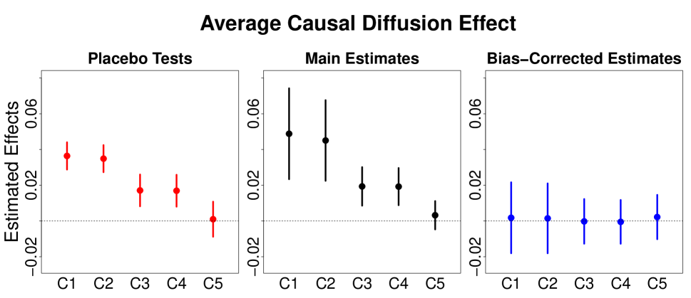
(a) (b) (c)

Figure 4: Placebo Tests, Main Estimates, and Bias-Corrected Estimates of the ACDE.
Note: Figures (a), (b) and (c) present results from the placebo tests, estimates of the ACDE under the no omitted confounders assumption, and estimates from bias-corrected estimators with 95% confidence intervals, respectively.

On the basis of these results from the placebo tests, we can now investigate estimates of the ACDE from the main model (equation (12)) in Figure 4 (b). For the first two cases (C1 and C2), estimates are as large as $5$ percentage points, but the placebo tests suggest that these estimates are heavily biased. Similarly, while the next two cases show point estimates of around $2$ percentage points, they are also likely to be biased. When we focus on the fifth control set, which produces a placebo estimate close to zero, a point estimate of the ACDE is smaller than $1$ percentage point, and its 95% confidence interval covers zero. The comparison between this more credible estimate and the one from the fourth set shows that an estimate of the ACDE can suffer from $100$% bias by missing just one variable. This demonstrates the importance of bias detection in causal diffusion analysis.

Although the proposed placebo tests suggest that the fifth control successfully adjusts for relevant confounders in this analysis, it is often infeasible to find such control sets in many other applications. To address these common scenarios, we now examine whether researchers could obtain similar results using a bias-corrected estimator even with control sets that reject the null hypothesis of the placebo test.

Figure 4 (c) shows that bias-corrected estimates are similar regardless of the selection of control variables and they all cover the most credible point estimate from the fifth control set. Even though the proposed placebo test detected a large amount of bias, researchers can obtain credible estimates by correcting the biases in this example.

These results suggest that, in contrast to existing studies (Braun, 2011; Jäckle and König, 2016), the ACDE on the incidence of hate crimes is small when averaging over all counties in Germany. In the next subsection, we show that the spatial diffusion of hate crimes is concentrated among a small subset of counties that have a higher proportion of school dropouts.

5.3 Heterogeneous Diffusion Effects by Education

Now, we extend the previous analysis by considering the types of counties that are more susceptible to the diffusion of hate crimes. In particular, we examine the role of education. Given rich qualitative and quantitative evidence that hate crime is often a problem of young people, it is critical to take into account one of the most important institutional contexts around them, i.e., schooling. The literature has discussed at least three mechanisms through which education can reduce the risk of hate crimes. First, education increases economic returns to current and future legitimate work, thereby raising the opportunity cost of committing hate crimes (e.g., Lochner and Moretti, 2004). Second, education may change the psychological costs associated with hate crimes. More educated people tend to have lower levels of ethnocentrism and place more emphasis on cultural diversity (Hainmueller and Hiscox, 2007). Finally, schooling has incapacitation effects – keeping adolescents busy and off the street, thereby directly reducing the chances of committing crimes (Jacob and Lefgren, 2003).

Building on the literature above, we investigate whether local educational contexts condition the spatial diffusion dynamics of hate crimes. We use a proportion of school dropouts without a secondary school diploma as a measure of local educational performance. To better disentangle the education explanation, we analyze East Germany and West Germany separately because they have substantially different distributions of proportions of school dropouts (counties in East Germany have much higher proportions of school dropouts). Here we report results from East Germany and provide those for West Germany in Appendix D. In particular, we estimate the conditional average causal diffusion effects (conditional ACDEs) for counties that have high and low proportions of school dropouts without a secondary school diploma. We use $9\%$ as a cutoff for high and low proportions of school dropouts, which is approximately the median value in East Germany. We add an interaction term between the treatment variable and this indicator variable to the original model in equation (12) and to the original placebo model in equation (13).

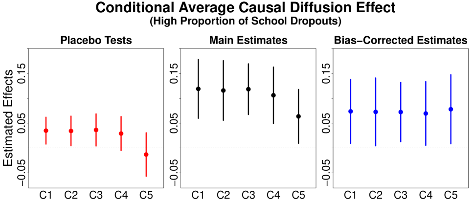
(a) (b) (c)

Figure 5: Placebo Tests, Main Estimates, and Bias-Corrected Estimates of the conditional ACDE for counties with a high proportion of school dropouts. Note: Figures (a), (b) and (c) present results from the placebo tests, estimates of the conditional ACDE under the no omitted confounders assumption, and estimates from bias-corrected estimators with 95% confidence intervals, respectively.

Figure 5 presents results for the conditional ACDE for counties that have a higher proportion of school dropouts. Similar to the case of the ACDE estimation, Figure 5 (a) shows strong concerns of biases in the first four sets of control variables. Even though a 95% confidence interval of the fourth estimate covers zero, its point estimate is far from zero (around $4$ percentage points). In contrast, the placebo test suggests that the fifth control set adjusts for relevant confounders where a placebo estimate is close to zero.

Based on results from the placebo tests, we examine estimates from the main model in Figure 5 (b). The first four sets, likely to be biased, exhibit large point estimates, larger than $10$ percentage points. More interestingly, even with the most credible fifth control set, a point estimate is as large as $6$ percentage points and is statistically significant. This effect size is substantively important given that it is about one-fourth of the sample average outcome in this subset ($26\%$). Bias-corrected estimates in Figure 5 (c) confirm that the conditional ACDE for counties with a higher proportion of school dropouts is large and similar regardless of the selection of control sets.

When we estimate the conditional ACDE for counties that have a lower proportion of school dropouts, effects are close to zero and their 95% confidence intervals cover zero, as the education hypothesis expects (see Appendix D). Causal diffusion effects are also precisely estimated to be zero in West Germany, where the proportions of school dropouts are much lower than East Germany. This additional analysis suggests that the spatial diffusion dynamics of hate crimes operate only in places with low educational performance and thus, prevention policies can have positive multiplier effects only when targeting areas with low educational performance.

6 Concluding Remarks

Causal diffusion dynamics have been an integral part of many social and biomedical science theories. Given that spatial and network panel data have become increasingly common, it is essential to develop methodologies to draw causal inference for diffusion effects. However, causal diffusion analysis has been challenging due to two well-known types of biases, i.e., contextual confounding and homophily bias. Recognizing that causal inference for diffusion effects is generally impossible without further assumptions (Shalizi and Thomas, 2011; VanderWeele and An, 2013; Ogburn, 2018), this paper examines the identification of causal diffusion effects under a new assumption of structural stationarity. This structural stationarity requires the existence of causal relationships among variables — not the effect or sign of such relationships — to be stable over time. Importantly, our approach based on the structural stationarity differs from a traditional DAG-based approach in that we only assume a class of dynamic causal DAGs, instead of a specific causal DAG. In particular, we develop methodologies valid for any causal DAGs within this general, large class of dynamic causal DAGs. Thus, the structural stationarity allows us to clearly encode assumptions about the underlying diffusion process without sacrificing its practical applicability.

Under the structural stationarity, we first propose a statistical placebo test that can detect a wide class of biases, including contextual confounding and homophily bias. Then, we develop a difference-in-differences style estimator that can directly correct biases under an additional parametric assumption. Applying the proposed methods to geo-coded hate crime data, we examined the spatial diffusion of hate crimes in Germany. After removing upward bias in previous studies, we found that the average effect of spatial diffusion is small, in contrast to recent quantitative analyses (Braun, 2011; Jäckle and König, 2016). The investigation of heterogeneous effects, however, revealed that the spatial diffusion effect of hate crimes is large in areas that have a high proportion of school dropouts. This empirical analysis demonstrates the large differences in substantive conclusions that can result from contextual confounding. By directly accounting for these biases, the proposed placebo test and bias-corrected estimator help researchers make more credible causal inference for diffusion studies.

There are a number of possible future extensions. First, whereas we propose an extension of the difference-in-differences estimator to causal diffusion analysis, future research should also investigate how to incorporate into causal diffusion analysis other popular tools developed for estimating the average treatment effect in panel data settings, such as synthetic control methods (Abadie et al., 2010). In addition, to further disentangle different channels of diffusion effects, it is of interest to study the intersection of the causal mediation analysis (Robins and Greenland, 1992; Pearl, 2001; Imai et al., 2010; VanderWeele, 2015) and the causal diffusion analysis (e.g., Ogburn and VanderWeele, 2014). With this extension, researchers can analyze, for example, micromechanisms of hate crime diffusion.

Supplementary Appendix

Appendix A Proofs

A.1 Proof of Theorem 1

In this proof, we use $\mathbf{C}$ and $\mathbf{C}^{P}$ to denote $\mathbf{C}_{i,t+1}$ and $\mathbf{C}^{P}_{i,t+1}$ for notational simplicity.

A.1.1 Setup

Given that control set $\mathbf{C}$ are defined to be pre-treatment, theoretical results on causal DAGs (Pearl, 1995; Shpitser et al., 2012) imply that $Y_{i,t+1}(d)\ \mbox{$\perp\!\!\!\perp$}\ \{Y_{jt}\}_{j\in\mathcal{N}_{i}}\mid\mathbf{C}$ is equivalent to no unblocked back-door paths from $\{Y_{jt}\}_{j\in\mathcal{N}_{i}}$ to $Y_{i,t+1}$ with respect to $\mathbf{C}$ in causal DAG $\mathcal{G}$ (see Lemma 1). Additionally, $Y_{it}(d)\ \mbox{$\perp\!\!\!\perp$}\ \{Y_{jt}\}_{j\in\mathcal{N}_{i}}\mid\mathbf{C}^{P}$ is equivalent to no unblocked back-door paths from $\{Y_{jt}\}_{j\in\mathcal{N}_{i}}$ to $Y_{it}$ with respect to $\mathbf{C}^{P}$ in causal DAG $\mathcal{G}$. Under the sequential consistency assumption (Assumption 1), $Y_{it}=Y_{it}(d)$ for any $d$. Therefore, $Y_{it}\ \mbox{$\perp\!\!\!\perp$}\ \{Y_{jt}\}_{j\in\mathcal{N}_{i}}\mid\mathbf{C}^{P}$ is equivalent to no unblocked back-door paths from $\{Y_{jt}\}_{j\in\mathcal{N}_{i}}$ to $Y_{it}$ with respect to $\mathbf{C}^{P}$ in causal DAG $\mathcal{G}$.

The theorem requires one regularity condition – the violation of the no omitted confounders assumption, if any, is proper. Intuitively, it means that bias (i.e., the violation of the no omitted confounders assumption) is in fact driven by omitted variables. Bias is not proper when the only source of bias is the misadjustment of the lag structure of observed covariates. Importantly, contextual confounding and homophily bias are proper, and hence within the scope of this theorem.

Definition 4 (Proper Bias).

Suppose control set $\mathbf{C}$ does not satisfy Assumption 2. This violation (bias) is defined to be proper when it satisfies the following condition: If control set $\mathbf{C}_{i,t+1}$ cannot block all back-door paths from $\{Y_{jt}\}_{j\in\mathcal{N}_{i}}$ to $Y_{i,t+1}$, there is at least one back-door path that any subset of the following set cannot block.

$$\{\mathbf{C}_{i,t+1},\mathbf{C}_{i,t+1}^{(-1)},\mathbf{C}_{i,t+1}^{(+1)},\{Y_{j,t-1}\}_{j\in\mathcal{N}_{i}}\},$$

where $\mathbf{C}_{i,t+1}^{(-1)}$ and $\mathbf{C}_{i,t+1}^{(+1)}$ are a lag and a lead of the time-dependent variables in $\mathbf{C}_{i,t+1}$.

A.1.2 Bias $\rightarrow$ Dependence in Placebo Test

Here, we show that when set $\mathbf{C}$ cannot block all back-door paths from $\{Y_{jt}\}_{j\in\mathcal{N}_{i}}$ to $Y_{i,t+1}$, set $\mathbf{C}^{P}$ cannot block all back-door paths from $\{Y_{jt}\}_{j\in\mathcal{N}_{i}}$ to $Y_{it}$.

Step 1 (Proper Bias):

Given the assumption that the set $\mathbf{C}$ is proper, set $\mathbf{C}^{P}$ cannot block all back-door paths from $\{Y_{jt}\}_{j\in\mathcal{N}_{i}}$ to $Y_{i,t+1}$ because $\mathbf{C}^{P}$ is a subset of $\{\mathbf{C},\mathbf{C}^{(-1)},\mathbf{C}^{(+1)},\{Y_{j,t-1}\}_{j\in\mathcal{N}_{i}}\}.$

Step 2 (Set up the main unblocked back-door path to investigate):

Let $\pi$ be a back-door path from $\{Y_{jt}\}_{j\in\mathcal{N}_{i}}$ to $Y_{i,t+1}$ that both $\mathbf{C}$ and $\mathbf{C}^{P}$ and any subset of $\{\mathbf{C},\mathbf{C}^{(-1)},\mathbf{C}^{(+1)},\{Y_{j,t-1}\}_{j\in\mathcal{N}_{i}}\}$ cannot block. Without loss of generality, we assume that this unblocked back-door path starts with an arrow pointing to $Y_{kt}$ where $k\in\mathcal{N}_{i}$ and it ends with an arrow pointing to $Y_{i,t+1}$.

Step 3 (Case I. the last node of the unblocked back-door path is time-independent):

First, consider a case in which the last variable in an unblocked back-door path has a directed arrow pointing to $Y_{i,t+1}$ and time-independent. Let ($Z$, $Y_{i,t+1}$) denote the last two node path segment on $\pi$ where $Z$ is a time-independent variable and there exists a directed arrow from $Z$ to $Y_{i,t+1}$. Note that we do not put any individual index to $Z$ because the proof holds for any index. Since this is an unblocked path, $Z$ is not in $\mathbf{C}^{P}$ and there is an unblocked back-door path from $Y_{kt}$ to $Z$. Since $Z$ is time-independent, there is a directed arrow from $Z$ to $Y_{it}$ by the structural stationarity (Assumption 3). Therefore, set $\mathbf{C}^{P}$ cannot block this back-door path from $Y_{kt}$ to $Y_{it}$.

Step 4 (Case II. the last node of the unblocked back-door path is time-dependent):

Next, consider the case in which the last variable in an unblocked back-door path points to $Y_{i,t+1}$ and time-dependent. Let ($B$, $X_{t+1}$, $Y_{i,t+1}$) denote the last three node path segment on $\pi$ where $X_{t+1}$ is a time-dependent direct cause of $Y_{i,t+1}$. Note that we do not put any individual index to $X_{t+1}$ because the proof holds for any index. $X_{t},X_{t+1}\not\in\mathbf{C}^{P}$ because $X_{t+1}\not\in\mathbf{C}$ (see Lemma 2 in Section A.2).

Step 4.1 (sub-Case: the second last node is time-independent):

First, assume $B$ is time-independent. Then, because a causal DAG satisfies the structural stationarity (Assumption 3), $X_{t}$ and $B$ have the same relationship as the one between $X_{t+1}$ and $B$. In addition, since there is an unblocked path from $Y_{kt}$ to $X_{t+1}$ to through $B$, there exists an unblocked path from $Y_{kt}$ to $X_{t}$ through $B$. Given that there exists a directed arrow from $X_{t+1}$ to $Y_{i,t+1}$, there exists a directed arrow from $X_{t}$ to $Y_{it}$. Therefore, there is an unblocked back-door path from $Y_{kt}$ to $Y_{it}$.

Step 4.2 (sub-Case: the second last node is time-dependent):

Next, assume $B$ is time-dependent and therefore we use $B_{t+1}$. First, we show that whenever $B$ is time-dependent, then the directed arrow is always from $X_{t+1}$ to $B_{t+1}.$ Suppose there is a directed arrow from $B_{t+1}$ to $X_{t+1}.$ If $B_{t+1}$ in $\mathbf{C}^{P}$, then this back-door is blocked (therefore, choose another $\pi$). So, $B_{t+1}$ is not in $\mathbf{C}^{P}$. Therefore, we can collapse $B_{t+1}$ into $X_{t+1}$, meaning that if $B$ is time dependent, then the directed arrow is always from $X_{t+1}$ to $B_{t+1}.$

Now, suppose there is a directed arrow from $X_{t+1}$ to $B_{t+1}.$ We know there exists an unblocked path from $Y_{kt}$ to $X_{t+1}$ through $B_{t+1}$. Now, because $Y_{it}\leftarrow X_{t}\rightarrow X_{t+1}\rightarrow B_{t+1}$, there is an unblocked back-door path from $Y_{kt}$ to $Y_{it}$ because the underlying causal DAG satisfies the structural stationarity.

A.1.3 No Bias $\rightarrow$ Independence in Placebo Test

Next, we prove that when set $\mathbf{C}$ can block all back-door paths from $\{Y_{jt}\}_{j\in\mathcal{N}_{i}}$ to $Y_{i,t+1}$, set $\mathbf{C}^{P}$ can block all back-door paths from $\{Y_{jt}\}_{j\in\mathcal{N}_{i}}$ to $Y_{it}.$ We show the contraposition: when there is a back-door path from $\{Y_{jt}\}_{j\in\mathcal{N}_{i}}$ to $Y_{it}$ that set $\mathbf{C}^{P}$ cannot block, set $\mathbf{C}$ cannot block all back-door paths from $\{Y_{jt}\}_{j\in\mathcal{N}_{i}}$ to $Y_{i,t+1}$. Since $\mathbf{C}$ does not include any $\mbox{Des}(Y_{kt})$, we know $\mathbf{C}^{P}$ also does not include any $\mbox{Des}(Y_{kt}).$ Also, by definition, $\mathbf{C}^{P}$ does not include any $\mbox{Des}(Y_{it}).$ Therefore, without loss of generality, we can focus on unblocked back-door paths that start with an arrow pointing to $Y_{kt}$ where $k\in\mathcal{N}_{i}$ and end with an arrow pointing to $Y_{it}$.

Step 1 (Control Set cannot block all back-door paths to the Placebo outcome):

First, we show that when there is a back-door path from $Y_{kt}$ to $Y_{it}$ that set $\mathbf{C}^{P}$ cannot block, set $\mathbf{C}$ cannot block all back-door paths from $Y_{kt}$ to $Y_{it}$. From set $\mathbf{C}^{P}$ to set $\mathbf{C}$, we need to (1) add $\mbox{Des}(Y_{it})$ and (2) remove $\mathbf{C}^{(-1)}$ and $\{Y_{j,t-1}\}_{j\in\mathcal{N}_{i}}$. We show here that this process cannot block a back-door path that set $\mathbf{C}^{P}$ cannot block. The step (1) cannot block the back-door path because adding $\mbox{Des}(Y_{it})$ cannot block a back-door path from $Y_{kt}$ to $Y_{it}$ unblocked by set $\mathbf{C}^{P}$ (see Lemma 3 in Section A.2). For (2), we first check whether removing $X_{t}\in\mathbf{C}^{(-1)}$ can block a back-door path that set $\mathbf{C}^{P}$ cannot block. To begin with, we can remove $X_{t}$ because $X_{t+1}\in\mathbf{C}$. Removing variables $X_{t}$ can be helpful if $X_{t}$ is a collider or a descendant of a collider for a back-door path. However, if so, $X_{t+1}$ is a descendant of a collider and it is in set $\mathbf{C}$ and therefore, removing $X_{t}$ cannot block any additional paths. Next, we need to check whether removing a variable $B\in\{Y_{j,t-1}\}_{j\in\mathcal{N}_{i}}$ can block the back-door path that the set $\mathbf{C}^{P}$ cannot block. Removing variable $B$ can be helpful if $B$ is a collider or a descendant of a collider for a back-door path. If so, there is an unblocked back-door path (with respect to $\mathbf{C}^{P}$) that starts with an arrow pointing to $B$ and ends with an arrow pointing to $Y_{it}$, i.e., $B\leftarrow\ldots\rightarrow Y_{it}.$ Since $B$ has a directed arrow pointing to $Y_{kt}$, removing $B$ unblock a new back-door path from $Y_{kt}$ through $B$, which points to $Y_{it}$. Although this unblocked back-door path with respect to $\mathbf{C}$ is different from the unblocked back-door path with respect to $\mathbf{C}^{P}$, the paths are the same after node $B$ and therefore at least the last three nodes are the same. Therefore, we can use $\pi$ to be a back-door from $Y_{kt}$ to $Y_{it}$ that both sets $\mathbf{C}$ and $\mathbf{C}^{P}$ cannot block.

Step 2 (Case I: the last node of the unblocked back-door path is time-independent):

Consider the case in which the last two nodes are $(Z\rightarrow Y_{it})$ and $Z$ is time-independent. Then, since $Z\rightarrow Y_{i,t+1}$ from the structural stationarity (Assumption 3), set $\mathbf{C}$ cannot block this back-door.

Step 3 (Case II: the last node of the unblocked back-door path is time-dependent):

Next, consider the case in which the last two nodes are $(X_{t}\rightarrow Y_{it}).$ Since $X_{t}\not\in\mathbf{C}^{P}$ and $X_{t}\not\in\mbox{Des}(Y_{it})$, $X_{t},X_{t+1}\not\in\mathbf{C}.$ Therefore, set $\mathbf{C}$ cannot block $Y_{kt}\leftarrow\cdots X_{t}\rightarrow X_{t+1}\rightarrow Y_{i,t+1}.$

A.2 Proof of Lemmas used for Theorem 1

Here, we prove all the lemmas used to prove Theorem 1.

Lemma 1 (Equivalence between Back-Door Criteria and No Omitted Confounder Assumption (Shpitser et al., 2012)).

For a pretreatment control set $\mathbf{C}$, the following two statements hold.

1. If a set $\mathbf{C}$ satisfies the back-door criterion with respect to $(Y_{i,t+1},\{Y_{jt}\}_{j\in\mathcal{N}_{i}})$ in causal DAG $\mathcal{G}$, then $Y_{i,t+1}(d)\ \mbox{$\perp\!\!\!\perp$}\ \{Y_{jt}\}_{j\in\mathcal{N}_{i}}\ \mid\mathbf{C}$ holds in every causal model inducing causal DAG $\mathcal{G}$ (Pearl, 1995).

2. If $Y_{i,t+1}(d)\ \mbox{$\perp\!\!\!\perp$}\ \{Y_{jt}\}_{j\in\mathcal{N}_{i}}\mid\mathbf{C}$ holds in every causal model inducing causal DAG $\mathcal{G}$, then a set $\mathbf{C}$ satisfies the back-door criterion with respect to $(Y_{i,t+1},\{Y_{jt}\}_{j\in\mathcal{N}_{i}})$ in causal DAG $\mathcal{G}$ (Shpitser et al., 2012).

Lemma 2.

$X_{t+1}\not\in\mathbf{C}\rightarrow X_{t},X_{t+1}\not\in\mathbf{C}^{P}.$

Proof

First, we show that $X_{t},X_{t+1},X_{t+2}\not\in\mathbf{C}$ because set $\mathbf{C}$ is proper. It is because if $X_{t}$ or $X_{t+2}$ are in $\mathbf{C}$, then the lag adjustment of the control set $\mathbf{C}$ can block this path. If this path is the only back-door path, then $\mathbf{C}$ is not proper. If there is another back-door path that any subset of $\{\mathbf{C},\mathbf{C}^{(-1)},\mathbf{C}^{(+1)},\{Y_{j,t-1}\}_{j\in\mathcal{N}_{i}}\}$ cannot block, choose it as $\pi$.

Next, we show that $X_{t},X_{t+1}\not\in\mathbf{C}^{P}$. There are three ways for a variable to be in the placebo set $\mathbf{C}^{P}$. We discuss them in order. First, a variable can be in the placebo set because it was already in the control set. We know $X_{t},X_{t+1}\not\in\mathbf{C}$, so this option is not feasible. Second, a variable can be in the placebo set because it is a lag of the original control variables. Given that $X_{t+1},X_{t+2}$ are not in the control set, this option is also not feasible. Finally, a variable can be in the placebo set because it is a lag of the treatment variable. (a) It is important to notice that $X_{t}\notin\{Y_{j,t-1}\}_{j\in\mathcal{N}_{i}}$ because $X_{t+1}\notin\{Y_{jt}\}_{j\in\mathcal{N}_{i}}$ (i.e., the treatment cannot be the last node of the unblocked back-door path). (b) Now, we verify $X_{t+1}\notin\{Y_{j,t-1}\}_{j\in\mathcal{N}_{i}}$. First, this back-door path can be blocked by a subset of $\{\mathbf{C},\mathbf{C}^{(-1)},\mathbf{C}^{(+1)},\{Y_{j,t-1}\}_{j\in\mathcal{N}_{i}}\}$. If this back-door is the only unblocked back-door, set $\mathbf{C}$ is not proper, therefore this is contradictory. If there is another back-door path that both $\mathbf{C}$ and $\mathbf{C}^{P}$ cannot block, choose it as $\pi$.

Lemma 3.

Adding $\mbox{Des}(Y_{it})$ cannot block a back-door path from $Y_{kt}$ to $Y_{it}$ unblocked by set $\mathbf{C}^{P}$.

Proof

Suppose controlling for $\mbox{Des}(Y_{it})$ can block a back-door path from $Y_{kt}$ to $Y_{it}$ that the original set $\mathbf{C}^{P}$ cannot block. Since $\mathbf{C}^{P}$ does not include any $\mbox{Des}(Y_{kt})$ or $\mbox{Des}(Y_{it})$, this unblocked back-door path contains an arrow pointing to $Y_{it}$.

Step 1 (Set up the main node $B$):

At least one of $\mbox{Des}(Y_{it})$ is a non-collider on this path given that controlling for $\mbox{Des}(Y_{it})$ can block this path. Let $B$ be such a variable and focus on one arrow pointing out from the node $B$.

Step 2 (Case I. Consider one side of the main node $B$):

First, suppose this direction leads to $Y_{it}$. Then, since $B$ is a $\mbox{Des}(Y_{it}),$ a directed path from node $B$ to $Y_{it}$ cannot exist and therefore, there must be a collider on this direction of the path. Since this collider is also in $\mbox{Des}(Y_{it})$ and therefore not controlled in the original $\mathbf{C}^{P}$, this back-door is blocked by set $\mathbf{C}^{P}.$

Step 3 (Case II. Consider the other side of the main node $B$):

Next, consider the direction that leads to $Y_{kt}.$ Then, since $Y_{it}$ is not a cause of $Y_{kt},$ a directed path from node $B$ to $Y_{kt}$ cannot exist and therefore, there must be a collider on this direction of the path. Since this collider is also in $\mbox{Des}(Y_{it})$ and therefore not controlled in the original $\mathbf{C}^{P}$, this back-door is blocked by set $\mathbf{C}^{P}.$ Hence, this is contradiction. This proves that controlling for $\mbox{Des}(Y_{it})$ cannot block a back-door path from $Y_{kt}$ to $Y_{it}$ that set $\mathbf{C}^{P}$ cannot block.

A.3 Placebo Test as Joint Test

In this section, we clarify a relationship between the placebo test and the sequential consistency (Assumption 1). While we assume the sequential consistency in Theorem 1 to assess the no omitted confounders assumption, a simple proof can show that the proposed placebo test can also be viewed as a joint test of the sequential consistency assumption and the no omitted confounders assumption under the structural stationarity. Formally,

Lemma 4 (Equivalence between Identification Assumptions and Conditional Independence of Simultaneous Outcomes).

Under Assumption 3,

$$\begin{cases}\ \text{Sequential Consistency (Assumption~{}\ref{seq})}\\[2.0pt] Y_{i,t+1}(d)\ \mbox{$\perp\!\!\!\perp$}\ \{Y_{jt}\}_{j\in\mathcal{N}_{i}}\mid\mathbf{C}_{i,t+1}\end{cases}{\vspace{-0.05in}\Longleftrightarrow}\ \ \ Y_{it}\ \mbox{$\perp\!\!\!\perp$}\ \{Y_{jt}\}_{j\in\mathcal{N}_{i}}\mid\mathbf{C}_{i,t+1}^{P}.$$

This lemma shows that researchers can assess not only the assumption of no omitted confounders (Assumption 2) but also the sequential consistency assumption (Assumption 1) together. That is, researchers can jointly detect simultaneity bias and omitted variable bias. When the conditional independence of simultaneous outcomes holds, it provides strong statistical evidence for both identification assumptions, i.e., the absence of simultaneity bias and omitted variable bias. In contrast, when we reject the null hypothesis of the placebo test, we cannot tell which assumption is violated. When the sequential consistency assumption is violated, the problem is more severe than omitted variable bias – causal diffusion effects are not well defined.

The proof of this lemma is essentially the same as the one for Theorem 1 and thus is omitted. One additional idea is that when the sequential consistency assumption is violated, there is no set of variables that can make simultaneous outcomes conditionally independent – the null hypothesis of the placebo test is always rejected.

A.4 Proof of Theorem 2

Below, we describe two lemmas useful for proving Theorem 2. For completeness, their proofs follow.

Lemma 5.

$$Y_{i,t+1}(d^{L})\ \mbox{$\perp\!\!\!\perp$}\ \{Y_{jt}\}_{j\in\mathcal{N}_{i}}\mid U_{i,t+1},\mathbf{C}_{i,t+1}\Longrightarrow Y_{i,t+1}(d^{L})\ \mbox{$\perp\!\!\!\perp$}\ \{Y_{jt}\}_{j\in\mathcal{N}_{i}}\mid U_{i,t+1},\mathbf{X}_{i,t+1},\mathbf{C}_{i,t+1}^{B}$$

Lemma 6.

Under Assumption 4,

$$\mathbb{E}[Y_{i,t+1}(d^{L})\mid D_{it}=d^{H},\mathbf{X}_{i,t+1}=\mathbf{x},\mathbf{C}_{i,t+1}^{B}=\mathbf{c}]-\mathbb{E}[Y_{i,t+1}(d^{L})\mid D_{it}=d^{L},\mathbf{X}_{i,t+1}=\mathbf{x},\mathbf{C}_{i,t+1}^{B}=\mathbf{c}]$$

$$= \mathbb{E}[Y_{it}(d^{L})\mid D_{it}=d^{H},\mathbf{X}_{it}=\mathbf{x},\mathbf{C}_{i,t+1}^{B}=\mathbf{c}]-\mathbb{E}[Y_{it}(d^{L})\mid D_{it}=d^{L},\mathbf{X}_{it}=\mathbf{x},\mathbf{C}_{i,t+1}^{B}=\mathbf{c}].$$

Proof of the theorem

Based on Lemma 6 and Assumptions 1 and 4,

$$\mathbb{E}[Y_{i,t+1}(d^{L})\mid D_{it}=d^{H},\mathbf{X}_{i,t+1}=\mathbf{x},\mathbf{C}_{i,t+1}^{B}=\mathbf{c}]$$

$$= \mathbb{E}[Y_{i,t+1}(d^{L})\mid D_{it}=d^{L},\mathbf{X}_{i,t+1}=\mathbf{x},\mathbf{C}_{i,t+1}^{B}=\mathbf{c}]$$

$$\quad+\mathbb{E}[Y_{it}(d^{L})\mid D_{it}=d^{H},\mathbf{X}_{it}=\mathbf{x},\mathbf{C}_{i,t+1}^{B}=\mathbf{c}]-\mathbb{E}[Y_{it}(d^{L})\mid D_{it}=d^{L},\mathbf{X}_{it}=\mathbf{x},\mathbf{C}_{i,t+1}^{B}=\mathbf{c}]$$

$$= \mathbb{E}[Y_{i,t+1}\mid D_{it}=d^{L},\mathbf{X}_{i,t+1}=\mathbf{x},\mathbf{C}^{B}_{i,t+1}=\mathbf{c}]$$

$$\quad+\mathbb{E}[Y_{it}\mid D_{it}=d^{H},\mathbf{X}_{it}=\mathbf{x},\mathbf{C}^{B}_{i,t+1}=\mathbf{c}]-\mathbb{E}[Y_{it}\mid D_{it}=d^{L},\mathbf{X}_{it}=\mathbf{x},\mathbf{C}^{B}_{i,t+1}=\mathbf{c}].$$

Therefore,

$$\mathbb{E}[Y_{i,t+1}(d^{H})-Y_{i,t+1}(d^{L})\mid D_{it}=d^{H}]$$

$$= \int\{\mathbb{E}[Y_{i,t+1}(d^{H})\mid D_{it}=d^{H},\mathbf{X}_{i,t+1},\mathbf{C}^{B}_{i,t+1}]$$

$$\qquad-\mathbb{E}[Y_{i,t+1}(d^{L})\mid D_{it}=d^{H},\mathbf{X}_{i,t+1},\mathbf{C}^{B}_{i,t+1}]\}dF_{\mathbf{X}_{i,t+1},\mathbf{C}^{B}_{i,t+1}\mid D_{it}=d^{H}}(\mathbf{x},\mathbf{c})$$

$$= \int\mathbb{E}[Y_{i,t+1}\mid D_{it}=d^{H},\mathbf{X}_{i,t+1},\mathbf{C}^{B}_{i,t+1}]dF_{\mathbf{X}_{i,t+1},\mathbf{C}^{B}_{i,t+1}\mid D_{it}=d^{H}}(\mathbf{x},\mathbf{c})$$

$$-\bigl{\{}\mathbb{E}[Y_{i,t+1}\mid D_{it}=d^{L},\mathbf{X}_{i,t+1}=\mathbf{x},\mathbf{C}^{B}_{i,t+1}=\mathbf{c}]+\mathbb{E}[Y_{it}\mid D_{it}=d^{H},\mathbf{X}_{it}=\mathbf{x},\mathbf{C}^{B}_{i,t+1}=\mathbf{c}]$$

$$\quad-\mathbb{E}[Y_{it}\mid D_{it}=d^{L},\mathbf{X}_{it}=\mathbf{x},\mathbf{C}^{B}_{i,t+1}=\mathbf{c}]\bigr{\}}dF_{\mathbf{X}_{i,t+1},\mathbf{C}^{B}_{i,t+1}\mid D_{it}=d^{H}}(\mathbf{x},\mathbf{c})$$

$$= \int\bigl{\{}\mathbb{E}[Y_{i,t+1}\mid D_{it}=d^{H},\mathbf{X}_{i,t+1},\mathbf{C}^{B}_{i,t+1}]-\mathbb{E}[Y_{i,t+1}\mid D_{it}=d^{L},\mathbf{X}_{i,t+1},\mathbf{C}^{B}_{i,t+1}]\bigr{\}}dF_{\mathbf{X}_{i,t+1},\mathbf{C}^{B}_{i,t+1}\mid D_{it}=d^{H}}(\mathbf{x},\mathbf{c})$$

$$-\int\bigl{\{}\mathbb{E}[Y_{it}\mid D_{it}=d^{H},\mathbf{X}_{it},\mathbf{C}^{B}_{i,t+1}]-\mathbb{E}[Y_{it}\mid D_{it}=d^{L},\mathbf{X}_{it},\mathbf{C}^{B}_{i,t+1}]\bigr{\}}dF_{\mathbf{X}_{i,t+1},\mathbf{C}^{B}_{i,t+1}\mid D_{it}=d^{H}}(\mathbf{x},\mathbf{c}).$$

This completes the proof of Theorem 2 in cases where $U_{i,t+1}$ is time-dependent and affected by the outcome at time $t$. In Section A.4.3, we extend results to two other cases (1) when $U_{i,t+1}$ is time-dependent but is not affected by the outcome at time $t$ and (2) when unobserved confounder is time-independent $Z_{i}$.

A.4.1 Proof of Lemma 5

If we write out control set $\mathbf{C}$, the lemma can be rewritten as

$$Y_{i,t+1}(d^{L})\ \mbox{$\perp\!\!\!\perp$}\ \{Y_{jt}\}_{j\in\mathcal{N}_{i}}\mid U_{i,t+1},\mathbf{X}_{i,t+1},\mathbf{V}_{i,t+1},\mathbf{Z}_{i}$$

$$\Longrightarrow Y_{i,t+1}(d^{L})\ \mbox{$\perp\!\!\!\perp$}\ \{Y_{jt}\}_{j\in\mathcal{N}_{i}}\mid U_{i,t+1},\mathbf{X}_{i,t+1},\mathbf{V}_{i,t+1},\mathbf{V}_{it},\mathbf{Z}_{i},\{Y_{j,t-1}\}_{j\in\mathcal{N}_{i}}.$$

First, note that all variables in set $\{U_{i,t+1},\mathbf{X}_{i,t+1},\mathbf{V}_{i,t+1},\mathbf{V}_{it},\mathbf{Z}_{i},\{Y_{j,t-1}\}_{j\in\mathcal{N}_{i}}\}$ are neither affected by the potential outcome, $Y_{i,t+1}(d^{L})$, nor affected by the treatment $\{Y_{jt}\}_{j\in\mathcal{N}_{i}}$. The difference between the conditioning sets in the right- and left-hand sides is $\mathbf{V}_{it}$ and $\{Y_{j,t-1}\}_{j\in\mathcal{N}_{i}}.$ Including these variables can open back-door paths only when these variables are colliders for these new back-door paths. However, because a descendant of $\mathbf{V}_{it}$, $\mathbf{V}_{i,t+1}$, is in the conditioning set, it is contradictory if conditioning on $\mathbf{V}_{it}$ can open a new back-door path. Additionally, because $\{Y_{j,t-1}\}_{j\in\mathcal{N}_{i}}$ is a parent of the treatment $\{Y_{jt}\}_{j\in\mathcal{N}_{i}}$, it is contradictory if conditioning on $\{Y_{j,t-1}\}_{j\in\mathcal{N}_{i}}$ can open a new back-door path. Therefore, including $\mathbf{V}_{it}$ and $\{Y_{j,t-1}\}_{j\in\mathcal{N}_{i}}$ don’t open any back-door path, which completes the proof.

A.4.2 Proof of Lemma 6

Under Assumption 4,

$$\int_{\mathcal{C}}\{\mathbb{E}[Y_{i,t+1}(d^{L})|U_{i,t+1}=u_{1},\mathbf{X}_{i,t+1}=\mathbf{x},\mathbf{C}^{B}_{i,t+1}=\mathbf{c}]-\mathbb{E}[Y_{i,t+1}(d^{L})|U_{i,t+1}=u_{0},\mathbf{X}_{i,t+1}=\mathbf{x},\mathbf{C}^{B}_{i,t+1}=\mathbf{c}]\}$$

$$\qquad\times\{dF_{U_{i,t+1}\mid D_{it}=d^{H},\mathbf{X}_{i,t+1}=\mathbf{x},\mathbf{C}^{B}_{i,t+1}=\mathbf{c}}(u_{1})-dF_{U_{i,t+1}\mid D_{it}=d^{L},\mathbf{X}_{i,t+1}=\mathbf{x},\mathbf{C}^{B}_{i,t+1}=\mathbf{c}}(u_{1})\}$$

$$= \int_{\mathcal{C}}\{\mathbb{E}[Y_{it}(d^{L})|U_{it}=u_{1},\mathbf{X}_{it}=\mathbf{x},\mathbf{C}^{B}_{i,t+1}=\mathbf{c}]-\mathbb{E}[Y_{it}(d^{L})|U_{it}=u_{0},\mathbf{X}_{it}=\mathbf{x},\mathbf{C}^{B}_{i,t+1}=\mathbf{c}]\}$$

$$\qquad\times\{dF_{U_{it}\mid D_{it}=d^{H},\mathbf{X}_{it}=\mathbf{x},\mathbf{C}^{B}_{i,t+1}=\mathbf{c}}(u_{1})-dF_{U_{it}\mid D_{it}=d^{L},\mathbf{X}_{it}=\mathbf{x},\mathbf{C}^{B}_{i,t+1}=\mathbf{c}}(u_{1})\}.$$

Now we analyze each side of the equation.

$$\int_{\mathcal{C}}\{\mathbb{E}[Y_{i,t+1}(d^{L})|U_{i,t+1}=u_{1},\mathbf{X}_{i,t+1}=\mathbf{x},\mathbf{C}^{B}_{i,t+1}=\mathbf{c}]-\mathbb{E}[Y_{i,t+1}(d^{L})|U_{i,t+1}=u_{0},\mathbf{X}_{i,t+1}=\mathbf{x},\mathbf{C}^{B}_{i,t+1}=\mathbf{c}]\}$$

$$\qquad\times\{dF_{U_{i,t+1}\mid D_{it}=d^{H},\mathbf{X}_{i,t+1}=\mathbf{x},\mathbf{C}^{B}_{i,t+1}=\mathbf{c}}(u_{1})-dF_{U_{i,t+1}\mid D_{it}=d^{L},\mathbf{X}_{i,t+1}=\mathbf{x},\mathbf{C}^{B}_{i,t+1}=\mathbf{c}}(u_{1})\}$$

$$= \int_{\mathcal{C}}\mathbb{E}[Y_{i,t+1}(d^{L})|U_{i,t+1}=u_{1},\mathbf{X}_{i,t+1}=\mathbf{x},\mathbf{C}^{B}_{i,t+1}=\mathbf{c}]$$

$$\qquad\times\{dF_{U_{i,t+1}\mid D_{it}=d^{H},\mathbf{X}_{i,t+1}=\mathbf{x},\mathbf{C}^{B}_{i,t+1}=\mathbf{c}}(u_{1})-dF_{U_{i,t+1}\mid D_{it}=d^{L},\mathbf{X}_{i,t+1}=\mathbf{x},\mathbf{C}^{B}_{i,t+1}=\mathbf{c}}(u_{1})\}$$

$$= \int_{\mathcal{C}}\mathbb{E}[Y_{i,t+1}(d^{L})|D_{it}=d^{H},U_{i,t+1}=u_{1},\mathbf{X}_{i,t+1}=\mathbf{x},\mathbf{C}^{B}_{i,t+1}=\mathbf{c}]dF_{U_{i,t+1}\mid D_{it}=d^{H},\mathbf{X}_{i,t+1}=\mathbf{x},\mathbf{C}^{B}_{i,t+1}=\mathbf{c}}(u_{1})$$

$$\qquad-\int_{\mathcal{C}}\mathbb{E}[Y_{i,t+1}(d^{L})|D_{it}=d^{L},U_{i,t+1}=u_{1},\mathbf{X}_{i,t+1}=\mathbf{x},\mathbf{C}^{B}_{i,t+1}=\mathbf{c}]dF_{U_{i,t+1}\mid D_{it}=d^{L},\mathbf{X}_{i,t+1}=\mathbf{x},\mathbf{C}^{B}_{i,t+1}=\mathbf{c}}(u_{1})$$

$$= \mathbb{E}[Y_{i,t+1}(d^{L})|D_{it}=d^{H},\mathbf{X}_{i,t+1}=\mathbf{x},\mathbf{C}^{B}_{i,t+1}=\mathbf{c}]-\mathbb{E}[Y_{i,t+1}(d^{L})|D_{it}=d^{L},\mathbf{X}_{i,t+1}=\mathbf{x},\mathbf{C}^{B}_{i,t+1}=\mathbf{c}],$$

where the first equality follows from the fact that $\mathbb{E}[Y_{i,t+1}(d^{L})|U_{i,t+1}=u_{0},\mathbf{X}_{i,t+1}=\mathbf{x},\mathbf{C}^{B}_{i,t+1}=\mathbf{c}]$ does not include $u_{1}$, the second equality comes from Lemma 5, and the final from the rule of conditional expectations. Similarly,

$$\int_{\mathcal{C}}\{\mathbb{E}[Y_{it}(d^{L})|U_{it}=u_{1},\mathbf{X}_{it}=\mathbf{x},\mathbf{C}^{B}_{i,t+1}=\mathbf{c}]-\mathbb{E}[Y_{it}(d^{L})|U_{it}=u_{0},\mathbf{X}_{it}=\mathbf{x},\mathbf{C}^{B}_{i,t+1}=\mathbf{c}]\}$$

$$\qquad\times\{dF_{U_{it}\mid D_{it}=d^{H},\mathbf{X}_{it}=\mathbf{x},\mathbf{C}^{B}_{i,t+1}=\mathbf{c}}(u_{1})-dF_{U_{it}\mid D_{it}=d^{L},\mathbf{X}_{it}=\mathbf{x},\mathbf{C}^{B}_{i,t+1}=\mathbf{c}}(u_{1})\}.$$

$$= \mathbb{E}[Y_{it}(d^{L})\mid D_{it}=d^{H},\mathbf{X}_{it}=\mathbf{x},\mathbf{C}^{B}_{i,t+1}=\mathbf{c}]-\mathbb{E}[Y_{it}(d^{L})\mid D_{it}=d^{L},\mathbf{X}_{it}=\mathbf{x},\mathbf{C}^{B}_{i,t+1}=\mathbf{c}].$$

Taken together,

$$\mathbb{E}[Y_{i,t+1}(d^{L})\mid D_{it}=d^{H},\mathbf{X}_{i,t+1}=\mathbf{x},\mathbf{C}^{B}_{i,t+1}=\mathbf{c}]-\mathbb{E}[Y_{i,t+1}(d^{L})\mid D_{it}=d^{L},\mathbf{X}_{i,t+1}=\mathbf{x},\mathbf{C}^{B}_{i,t+1}=\mathbf{c}]$$

$$= \mathbb{E}[Y_{it}(d^{L})\mid D_{it}=d^{H},\mathbf{X}_{it}=\mathbf{x},\mathbf{C}^{B}_{i,t+1}=\mathbf{c}]-\mathbb{E}[Y_{it}(d^{L})\mid D_{it}=d^{L},\mathbf{X}_{it}=\mathbf{x},\mathbf{C}^{B}_{i,t+1}=\mathbf{c}].$$

A.4.3 Other cases

In Theorem 2, we consider cases in which $U_{i,t+1}$ is time-dependent and affected by the outcome at time $t$. Now we study two other cases (1) when $U_{i,t+1}$ is time-dependent but is not affected by the outcome at time $t$ and (2) when unobserved confounder is time-independent $Z_{i}$. For both cases, Assumption 4 needs to be modified accordingly, although their substantive meanings stay the same. The definition of the bias-corrected estimator is also the same. For case (1), define $\widetilde{U}_{i}\equiv(U_{i,t+1},U_{it})$ and for case (2), define $\widetilde{U}_{i}\equiv Z_{i}.$ Then, Assumption 4 is modified as follows.

1. Time-invariant effect of unobserved confounder $\widetilde{U}$: For all $u_{1},u_{0},\mathbf{x}$ and $\mathbf{c},$

   $$\mathbb{E}[Y_{i,t+1}(d^{L})\mid\widetilde{U}_{i}=u_{1},\mathbf{X}_{i,t+1}=\mathbf{x},\mathbf{C}^{B}_{i,t+1}=\mathbf{c}]-\mathbb{E}[Y_{i,t+1}(d^{L})\mid\widetilde{U}_{i}=u_{0},\mathbf{X}_{i,t+1}=\mathbf{x},\mathbf{C}^{B}_{i,t+1}=\mathbf{c}]$$

   $$= \mathbb{E}[Y_{it}(d^{L})\mid\widetilde{U}_{i}=u_{1},\mathbf{X}_{it}=\mathbf{x},\mathbf{C}^{B}_{i,t+1}=\mathbf{c}]-\mathbb{E}[Y_{it}(d^{L})\mid\widetilde{U}_{i}=u_{0},\mathbf{X}_{it}=\mathbf{x},\mathbf{C}^{B}_{i,t+1}=\mathbf{c}].$$

2. Time-invariant imbalance of unobserved confounder $\widetilde{U}$: For all $u,\mathbf{x}$ and $\mathbf{c},$

   $$\Pr(\widetilde{U}_{i}\leq u\mid D_{it}=d^{H},\mathbf{X}_{i,t+1}=\mathbf{x},\mathbf{C}^{B}_{i,t+1}=\mathbf{c})-\Pr(\widetilde{U}_{i}\leq u\mid D_{it}=d^{L},\mathbf{X}_{i,t+1}=\mathbf{x},\mathbf{C}^{B}_{i,t+1}=\mathbf{c})$$

   $$= \Pr(\widetilde{U}_{i}\leq u\mid D_{it}=d^{H},\mathbf{X}_{it}=\mathbf{x},\mathbf{C}^{B}_{i,t+1}=\mathbf{c})-\Pr(\widetilde{U}_{i}\leq u\mid D_{it}=d^{L},\mathbf{X}_{it}=\mathbf{x},\mathbf{C}^{B}_{i,t+1}=\mathbf{c}).$$

A.5 Extensions

A.5.1 Sensitivity Analysis

As Lemma 6 shows, Assumption 4 is equivalent to the following equality.

$$\mathbb{E}[Y_{i,t+1}(d^{L})\mid D_{it}=d^{H},\mathbf{X}_{i,t+1}=\mathbf{x},\mathbf{C}_{i,t+1}^{B}=\mathbf{c}]-\mathbb{E}[Y_{i,t+1}(d^{L})\mid D_{it}=d^{L},\mathbf{X}_{i,t+1}=\mathbf{x},\mathbf{C}_{i,t+1}^{B}=\mathbf{c}]$$

$$= \mathbb{E}[Y_{it}(d^{L})\mid D_{it}=d^{H},\mathbf{X}_{it}=\mathbf{x},\mathbf{C}_{i,t+1}^{B}=\mathbf{c}]-\mathbb{E}[Y_{it}(d^{L})\mid D_{it}=d^{L},\mathbf{X}_{it}=\mathbf{x},\mathbf{C}_{i,t+1}^{B}=\mathbf{c}],$$

which substantively means the time-invariant bias. However, this assumption might hold only approximately in applied settings. To assess the robustness of the bias-corrected estimates, we consider a sensitivity analysis. In particular, we introduce sensitivity parameter $\lambda$ as follows.

$$\frac{\mbox{B}_{t+1}(\mathbf{x},\mathbf{c})}{\mbox{B}_{t}(\mathbf{x},\mathbf{c})}=\lambda$$

where

$$\mbox{B}_{t+1}(\mathbf{x},\mathbf{c}) = \mathbb{E}[Y_{i,t+1}(d^{L})\mid D_{it}=d^{H},\mathbf{X}_{i,t+1}=\mathbf{x},\mathbf{C}_{i,t+1}^{B}=\mathbf{c}]-\mathbb{E}[Y_{i,t+1}(d^{L})\mid D_{it}=d^{L},\mathbf{X}_{i,t+1}=\mathbf{x},\mathbf{C}_{i,t+1}^{B}=\mathbf{c}],$$

$$\mbox{B}_{t}(\mathbf{x},\mathbf{c}) = \mathbb{E}[Y_{it}(d^{L})\mid D_{it}=d^{H},\mathbf{X}_{it}=\mathbf{x},\mathbf{C}_{i,t+1}^{B}=\mathbf{c}]-\mathbb{E}[Y_{it}(d^{L})\mid D_{it}=d^{L},\mathbf{X}_{it}=\mathbf{x},\mathbf{C}_{i,t+1}^{B}=\mathbf{c}].$$

The time-invariance assumption (Assumption 4) corresponds to $\lambda=1.$ Using this sensitivity parameter, we can re-define the bias-corrected estimator as follows.

$$\hat{\tau}_{\text{Main}}-\lambda\times\hat{\delta}_{\text{Placebo}}$$

Therefore, a sensitivity analysis is to compute the bias-corrected estimator for a range of plausible values of $\lambda$ and investigate whether substantive conclusions vary according to the choice of the sensitivity parameter.

A.5.2 Assumptions for Identification of ACDE

As we show in Section 4.3.3, Assumption 4 is sufficient for the identification of the ACDE for the treated. Here, we consider an extension of this assumption sufficient for the identification of the ACDE. In particular, we additionally assume the following equality, which is an extension of Assumption 4.1 to the case of potential outcomes $Y_{i}(d^{H}).$

Assumption 4.3

(Time-invariant effect of unobserved confounder $U$ on potential outcomes $Y_{i,t+1}(d^{H})$)

$$\mathbb{E}[Y_{i,t+1}(d^{H})|U_{i,t+1}=u_{1},\mathbf{X}_{i,t+1}=\mathbf{x},\mathbf{C}_{i,t+1}^{B}=\mathbf{c}]-\mathbb{E}[Y_{i,t+1}(d^{H})|U_{i,t+1}=u_{0},\mathbf{X}_{i,t+1}=\mathbf{x},\mathbf{C}_{i,t+1}^{B}=\mathbf{c}]$$

$$= \mathbb{E}[Y_{it}(d^{H})|U_{it}=u_{1},\mathbf{X}_{it}=\mathbf{x},\mathbf{C}_{i,t+1}^{B}=\mathbf{c}]-\mathbb{E}[Y_{it}(d^{H})|U_{it}=u_{0},\mathbf{X}_{it}=\mathbf{x},\mathbf{C}_{i,t+1}^{B}=\mathbf{c}],$$

for all $u_{1},u_{0},\mathbf{x}$ and $\mathbf{c}.$

Combining this assumption and Assumption 4.2, we obtain

$$\mathbb{E}[Y_{i,t+1}(d^{H})\mid D_{it}=d^{H},\mathbf{X}_{i,t+1}=\mathbf{x},\mathbf{C}^{B}_{i,t+1}=\mathbf{c}]-\mathbb{E}[Y_{i,t+1}(d^{H})\mid D_{it}=d^{L},\mathbf{X}_{i,t+1}=\mathbf{x},\mathbf{C}^{B}_{i,t+1}=\mathbf{c}]$$

$$= \mathbb{E}[Y_{it}(d^{H})\mid D_{it}=d^{H},\mathbf{X}_{it}=\mathbf{x},\mathbf{C}^{B}_{i,t+1}=\mathbf{c}]-\mathbb{E}[Y_{it}(d^{H})\mid D_{it}=d^{L},\mathbf{X}_{it}=\mathbf{x},\mathbf{C}^{B}_{i,t+1}=\mathbf{c}],$$

where the proof follows from Lemma 6. Using this result, we can additionally show the identification of the ACDE for units who received $d^{L}.$

$$\mathbb{E}[\hat{\tau}^{d^{L}}_{\text{BC}}] = \tau^{d^{L}}_{t+1}(d^{H},d^{L}),$$

under Assumption 4.2, and Assumption 4.3, where

$$\hat{\tau}^{d^{L}}_{\text{BC}} = \int\bigl{\{}\widehat{\mathbb{E}}[Y_{i,t+1}\mid D_{it}=d^{H},\mathbf{X}_{i,t+1},\mathbf{C}^{B}_{i,t+1}]-\widehat{\mathbb{E}}[Y_{i,t+1}\mid D_{it}=d^{L},\mathbf{X}_{i,t+1},\mathbf{C}^{B}_{i,t+1}]\bigr{\}}dF_{\mathbf{X}_{i,t+1},\mathbf{C}^{B}_{i,t+1}\mid D_{it}=d^{L}}(\mathbf{x},\mathbf{c})$$

$$-\int\bigl{\{}\widehat{\mathbb{E}}[Y_{it}\mid D_{it}=d^{H},\mathbf{X}_{it},\mathbf{C}^{B}_{i,t+1}]-\widehat{\mathbb{E}}[Y_{it}\mid D_{it}=d^{L},\mathbf{X}_{it},\mathbf{C}^{B}_{i,t+1}]\bigr{\}}dF_{\mathbf{X}_{i,t+1},\mathbf{C}^{B}_{i,t+1}\mid D_{it}=d^{L}}(\mathbf{x},\mathbf{c}).$$

The proof is analogous to Theorem 2. Finally, by combining this result and Theorem 2 with weights $\Pr(D_{it}=d^{H})$ and $\Pr(D_{it}=d^{L})$, we can get

$$\mathbb{E}[\hat{\tau}^{\ast}_{\text{BC}}] = \tau_{t+1}(d^{H},d^{L}).$$

under Assumption 4.1, Assumption 4.2, and Assumption 4.3, where

$$\hat{\tau}^{\ast}_{\text{BC}}\equiv\Pr(D_{it}=d^{H})\hat{\tau}_{\text{BC}}+\Pr(D_{it}=d^{L})\hat{\tau}^{d^{L}}_{\text{BC}}.$$

Appendix B Causal Directed Acyclic Graphs: Review

In the paper, we use a causal directed acyclic graph and nonparametric structural equations to represent causal relationships. Here, we review basic definitions and results. See Pearl (2000) for a comprehensive review. Following Pearl (1995), we define a causal directed acyclic graph (causal DAG) to be a set of nodes and directed edges among nodes such that the graph has no cycles and each node corresponds to a univariate random variable. Each random variable is given by its nonparametric structural equation. When there is a directed edge from one variable to another variable, the latter variable is a function of the former variable. For example, in a causal DAG in Figure A1 (a), four random variables $(A,B,C,D)$ are given by nonparametric structural equations in Figure A1 (b); $A=f_{A}(\epsilon_{A}),B=f_{B}(\epsilon_{B}),C=f_{C}(A,B,\epsilon_{C})$, and $D=f_{D}(A,B,C,\epsilon_{D}),$ where $f_{A},f_{B},f_{C}$ and $f_{D}$ are unknown nonparametric structural equations and $(\epsilon_{A},\epsilon_{B},\epsilon_{C},\epsilon_{D})$ are mutually independent errors. The node that a directed edge starts from is called the parent of the node that the edge goes into. The node that the edge goes into is the child of the node it comes from. If two nodes are connected by a directed path, the first node is the ancestor of every node on the path, and every node on the path is the descendant of the first node (Pearl, 2000). For example, node A is a parent of node C, and nodes C and D are descendants of node B. The requirement that the errors be mutually independent essentially means that there is no variable absent from the graph which, if included on the graph, would be a parent of two or more variables.

The nonparametric structural equations are general – random variables may depend on any function of their parents and variable-specific errors. They encode counterfactual relationships between the variables on the graph by recursively representing one-step-ahead counterfactuals. Under a hypothetical intervention setting $A$ to $a$, the distribution of the variables $B,C$, and $D$ are then recursively given by the nonparametric structural equations with $A=f_{A}(\epsilon_{A})$ replaced by $A=a$. Specifically, $B=f_{B}(\epsilon_{B}),\ C=C(a)=f_{C}(A=a,B,\epsilon_{C})$, and $D=D(a)=f_{D}(A=a,B,C=C(a),\epsilon_{D})$ where $C(a),D(a)$ are the counterfactual values of $C$ and $D$ when $A$ is set to $a$.

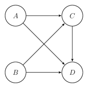
(a) A causal directed acyclic graph $\displaystyle A$ $\displaystyle=$ $\displaystyle f_{A}(\epsilon_{A})$ $\displaystyle B$ $\displaystyle=$ $\displaystyle f_{B}(\epsilon_{B})$ $\displaystyle C$ $\displaystyle=$ $\displaystyle f_{C}(A,B,\epsilon_{C})$ $\displaystyle D$ $\displaystyle=$ $\displaystyle f_{D}(A,B,C,\epsilon_{D})$ (b) A structural equation model

Figure A1: An Example of Causal DAGs and SEMs

Appendix C Simulation Study

In this section, we consider the performance of the proposed placebo test and bias-corrected estimator in a simulation study calibrated to the real hate crime data. In Section C.1, we show that (1) a placebo estimator is consistent for zero under the no omitted confounders assumption as Theorem 1 implies and (2) the statistical power of the proposed placebo test is comparable to an “oracle” test — test whether an estimated ACDE is statistically distinguishable from the true ACDE, which is available only in simulations. In Section C.2, we demonstrate that the bias-corrected estimator reduces bias and root mean squared error (RMSE) even under a slight violation of the time-invariance assumption (Assumption 4).

Setup.

To approximate realistic data generating processes, we use the same hate crime data as in the main application but focus on another important outcome, the number of attacks against refugee housing, which is also an important aspect of hate crimes studied in the literature. As for observed covariates, we include five major contextual variables; the number of refugees, the number of crimes per 100,000 inhabitants, per capita income, the unemployment rate, and the share of school leavers without lower secondary education graduation. We fit a linear regression with these five covariates, as in equation (8), to estimate the basic parameters of the data generating process.

We simulate a distance matrix $\mathbf{W}$ based on the stochastic block model (Holland et al., 1983) for each of the sample size $n\in\{100,500,1000,2000\}$. Each group consists of ten units and there exist $K=n/10$ groups. $K$ groups are divided into $L=K/5$ blocks. If units $i$ and $j$ are within the same group, $\Pr(W_{ij}=1)=0.8.$ If units $i$ and $j$ are within the same block but not in the same group, $\Pr(W_{ij}=1)=0.2.$ If units $i$ and $j$ are in different blocks, $\Pr(W_{ij}=1)=0.$ This setup is designed to ensure that the network dependency does not keep growing as the sample size grows. See Sävje et al. (2017) and Ogburn et al. (2017) for general discussions on network asymptotics.

We then simulate an unobserved contextual variable $U_{it}.$ In particular, we consider two scenarios; (1) time-invariant confounding where assumptions for both the placebo test and the bias-corrected estimator hold, and (2) structural stationarity where assumptions hold for the placebo test but the time-invariance assumption required for the bias-correction is violated. For the first scenario, we set unobserved contextual variable $U$ to be time-invariant where $U_{i}=\widetilde{U}_{k[i]}$ where $\tilde{U}_{k}\sim\mathcal{N}(0,0.5)$ and $k[i]$ is a group indicator for unit $i$. For the second scenario, we draw unobserved contextual variable $U$ as follows. $U_{it}=\widetilde{U}_{k[i],t}$ where $U_{k,t}=0.9U_{k,t-1}+\mathcal{N}(0,0.1)$ where $U_{k0}\sim\mathcal{N}(0,0.5).$

Given this setup, we sample potential outcomes using the following data generating process.

$$Y_{i,t+1}(D_{it})=\alpha+\tau D_{it}+\mathbf{X}_{i,t+1}^{\top}\beta+\gamma U_{i,t+1}+\epsilon_{i,t+1},$$ (1)

for sample size in each time period $n\in\{100,500,1000,2000\}$ and the total number of time periods $T=20$. $D_{it}\equiv\mathbf{W}_{i}^{\top}\mathbf{Y}_{t}$ indicates the treatment variable, five-dimensional vector $\mathbf{X}_{i,t+1}$ represents five observed covariates from the real hate crime data, $U_{i,t+1}$ is the unobserved contextual confounder affecting multiple units, and the error term $\epsilon_{i,t+1}$ follows the normal distribution, $\epsilon_{i,t+1}\sim\mathcal{N}(0,0.1)$. Coefficients {$\alpha=0.59,\tau=0.74,\beta=(0.75,-0.11,-0.28,-3.38,3.90)$} are based on estimated parameters from the real hate crime data. The effect of unobserved contextual confounder $U$ is set to $\gamma=0.1.$ Based on this data generating process, we conduct 5000 independent Monte Carlo simulations.

C.1 Placebo Test

First, we consider the consistency of the proposed placebo test under the no omitted confounders assumption. Theorem 1 implies that when the no omitted confounders assumption holds, the treatment variable and the lagged dependent variable are conditionally independent. In particular, we fit a placebo regression:

$$Y_{it}=\alpha_{0}+\delta D_{it}+\tau_{0}D_{i,t-1}+\mathbf{X}_{it}^{\top}\beta_{0}+\gamma_{0}U_{it}+\epsilon_{it}.$$ (2)

We expect that a test statistic $\widehat{\delta}$ is consistent for zero under the no omitted confounders assumption. The first row in Figure A2 presents the results. As Theorem 1 shows, under the no omitted confounders assumption, the placebo estimator $\widehat{\delta}$ converges to zero as the sample size grows. Because Theorem 1 only requires the structural stationarity, the placebo test is consistent under both scenarios.

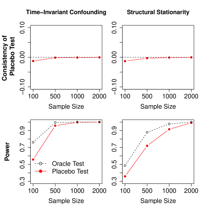
Figure A2: Simulation Results on Placebo Test. Note: The first row considers the consistency of the placebo test under the no omitted confounders assumption. The second row compares the statistical power of the proposed placebo test (solid red line) and the oracle test (dotted black line). The first and second columns correspond to the time-invariant confounding and the structural stationarity, respectively. Results are based on 5000 Monte Carlo draws using four sample sizes.

We also investigate the statistical power of the proposed placebo test when the no omitted confounders assumption is violated. We fit a placebo regression:

$$Y_{it}=\tilde{\alpha}_{0}+\tilde{\delta}D_{it}+\tilde{\tau}_{0}D_{i,t-1}+\mathbf{X}_{it}^{\top}\tilde{\beta}_{0}+\tilde{\epsilon}_{it}.$$ (3)

The key difference is that this regression now ignores contextual confounder $U_{it}$. Here, $\widehat{\tilde{\delta}}$ serves as a test statistic for the placebo test. We compare this to an oracle test where we fit the following main linear regression,

$$Y_{i,t+1}=\alpha_{m}+\tau_{m}D_{it}+\mathbf{X}_{i,t+1}^{\top}\beta_{m}+\xi_{i,t+1},$$ (4)

and test $H_{0}:\tau_{m}=\tau.$ This test is an “oracle” test because it is available only in the simulation where we know the true ACDE $\tau.$ The second row in Figure A2 presents the results. Even when the sample size is small, the proposed placebo test achieves more than 70% of the oracle test’s power. As the sample size grows, the proposed placebo test attains the statistical power as high as that of the oracle test. Given that the oracle test is available only in simulations where the true ACDE is known, these results suggest that the placebo test can serve as a powerful practical tool to detect biases in applied settings.

C.2 Bias-Corrected Estimator

In Section 4.3, we show that the proposed bias-corrected estimator can identify the ACDE for the treated under Assumption 4. Here, we investigate how much the bias-corrected estimator can reduce bias and RMSE even in settings where this required time-invariance assumption is slightly violated.

In particular, we compare an uncorrected estimator, which ignores unobserved contextual confounder $U$, and the proposed bias-corrected estimator under two scenarios; (1) time-invariant confounding and (2) structural stationarity. The time-invariance assumption required for the bias correction (Assumption 4) holds in the first but not in the second scenario.

Figure A3 presents the simulation results. In the time-invariant confounding case (the first column), whereas the bias in the conventional uncorrected estimator is about $0.12$, the bias in the proposed bias-corrected estimator is essentially $0$. The bias is corrected as Theorem 2 implies. The RMSE also significantly improves upon the uncorrected conventional estimator. The 95% confidence interval is close to its nominal coverage rate in contrast to that of the uncorrected estimator.

More importantly, even in the structural stationarity case (the second column in Figure A3) where the required assumption for the bias correction is slightly violated, the bias-corrected estimator shows reasonable performance. While the bias in the conventional uncorrected estimator is about $0.04$, the bias in the proposed bias-corrected estimator is less than $0.01$. Although the bias does not vanish, it reduces by about 80%. This benefit is also clear in the results of RMSE. Because the bias-corrected estimator tends to have a larger standard error, the RMSE of the bias-corrected estimator is bigger than the one of the uncorrected estimator when the sample size is small. However, as the sample size grows, the bias-corrected estimator outperforms the uncorrected estimator. Finally, as the required time-invariance assumption is violated, the coverage of the 95% confidence interval for the bias-corrected estimator is slightly smaller than its nominal coverage rate, but it attains more than 90% in contrast to the performance of the uncorrected estimator. These results suggest that the proposed bias-corrected estimator can reduce bias and RMSE in applied settings where the necessary assumption might hold only approximately.

Figure A3: Simulation Results on Bias-Corrected Estimator. Note: The first row compares the absolute bias of the uncorrected estimator (empty black square) and the bias-corrected estimator (solid blue circle). The second row examines the root mean squared error (RMSE) and the third row shows the coverage of the 95% confidence interval. The first and second columns correspond to the time-invariant confounding and the structural stationarity, respectively. Results are based on 5000 Monte Carlo draws using four sample sizes.

Appendix D Empirical Analysis in Section 5

D.1 Control Sets and Placebo Sets

We investigate five different control sets to illustrate how to use the proposed placebo test and bias-corrected estimator. Table A1 describes types of variables we use for those five control sets and their corresponding placebo sets. The column of “Main model” indicates variables used for control sets and the column of “Placebo model” indicates corresponding variables in placebo sets.

Type	Main Model	Placebo Model
Outcome	Physical Attackt+1	Physical Attackt
Treatment	Physical Attackt in Neighbors	Physical Attackt in Neighbors
A Control Set/A Placebo Set
1-3  Basic Variables	Physical Attackt	Physical Attackt-1
	Physical Attackt-1 in Neighbors	Physical Attackt-1,t-2 in Neighbors
	the number of neighbors	the number of neighbors
	variance of $\mathbf{W}_{i}$	variance of $\mathbf{W}_{i}$
1-3  Two-month Lags	Physical Attackt-1	Physical Attackt-2
1-3  Contextual Variables (annual)
Refugee variables	Total number of refugees	Total number of refugees
	Total number of foreign born	Total number of foreign born
Population variables	Population size	Population size
	Share of male inhabitants	Share of male inhabitants
Crime variables	Number of general crimes per 100,000 inhabitants	Number of general crimes per 100,000 inhabitants
	Percent of general crimes solved	Percept of general crimes solved
Economic variables	Number of newly registered business	Number of newly registered business
	Number of newly deregistered business	Number of newly deregistered business
	Number of insolvency	Number of insolvency
	per capita income	per capita income
	Number of employees with social security	Number of employees with social security
	Unemployment rate	Unemployment rate
Education variables	Share of school leavers	Share of school leavers
	without lower secondary education graduation	without lower secondary education graduation
Political variables	Turnout rate in 2013	Turnout rate in 2013
	Vote share of extreme right and	Vote share of extreme right and
	populist right-wing parties in 2013	populist right-wing parties in 2013

Table A1: Five Control Sets and Placebo Sets: Spatial Diffusion of Hate Crimes.

The first control set (C1) includes variables from “Basic Variables.” The second control set (C2) adds variables from “Two-month Lags” to the first control set. The third control set adds state fixed effects to the second control set. The fourth control set adds all the variables from “Contextual Variables,” which include variables on refugees, demographics, general crimes, economic indicators, education, and politics. Note that these contextual variables are measured only annually. The final fifth set adds the time trend variable as third-order polynomials to the fourth set.

D.2 Conditional ACDEs by Education

We present the distribution of proportions of school dropouts without a secondary school diploma, separately for East Germany and West Germany. Because these distributions are substantially different between them (Figure A4), we estimate the conditional ACDE by proportions of school dropouts, separately for the East and the West.

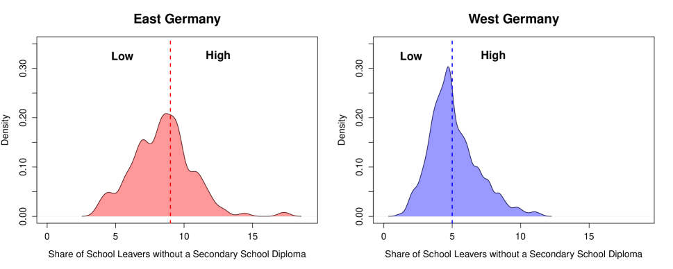
Figure A4: Distribution of Proportions of School Dropouts. Note: For East Germany, we use 9% as a cutoff for high and low proportions of school dropouts, which is approximately the median value in East Germany. For West Germany, we use 5% as a cutoff for high and low proportions of school dropouts, which is approximately the median value in West Germany.

Next, we present the conditional ACDE for counties in East Germany with low proportions of school dropouts. In contrast to Figure 5, estimates are small.

(a)                                     (b)                                     (c)

Figure A5: Results of the conditional ACDE (Low Proportion of School Dropouts, East). Note: Figure (a) shows that the last fifth set produces the smallest placebo estimate. Focusing on this fifth control set, a point estimate of the ACDE in Figure (b) is close to zero and its 95% confidence interval covers zero. Figure (c) shows that bias-corrected estimates are similar regardless of the selection of control variables and all of their 95% confidence intervals cover zero.

Now, we present the conditional ACDEs for counties in West Germany with high and low proportions of school dropouts. Given that proportions of school dropouts are lower in West Germany, estimates of the conditional ACDEs are small, in contrast to Figure 5.

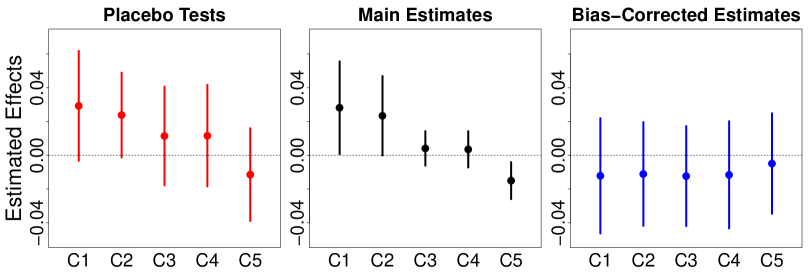
(a)                                     (b)                                     (c)

Figure A6: Results of the conditional ACDE (High Proportion of School Dropouts, West). Note: Figure (a) shows that the third, fourth and fifth sets produce small placebo estimates. Focusing on these sets, point estimates of the ACDE in Figure (b) are close to zero and sometimes negative. Figure (c) shows that bias-corrected estimates are similar regardless of the selection of control variables and all of their 95% confidence intervals cover zero.

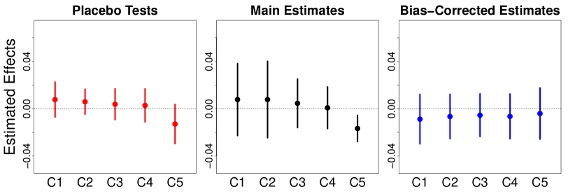
(a)                                     (b)                                     (c)

Figure A7: Results of the conditional ACDE (Low Proportion of School Dropouts, West). Note: Figure (a) shows that all the sets produce small placebo estimates. This is partly because there are few hate crimes in this area and hence, there is no variation in outcomes and treatments. In addition, point estimates of the ACDE in Figure (b) are close to zero and sometimes negative. Figure (c) shows that bias-corrected estimates are similar regardless of the selection of control variables and all of their 95% confidence intervals cover zero.

References

- Abadie et al. (2010) Abadie, A., Diamond, A., and Hainmueller, J. (2010). Synthetic Control Methods for Comparative Case Studies: Estimating the Effect of California’s Tobacco Control Program. Journal of the American Statistical Association, 105(490), 493–505.
- An (2015) An, W. (2015). Instrumental Variables Estimates of Peer Effects in Social Networks. Social Science Research, 50, 382–394.
- Anagnostopoulos et al. (2008) Anagnostopoulos, A., Kumar, R., and Mahdian, M. (2008). Influence and Correlation in Social Networks. In Proceedings of the 14th ACM SIGKDD International Conference on Knowledge Discovery and Data Mining, pages 7–15. ACM.
- Angrist (2014) Angrist, J. D. (2014). The Perils of Peer Effects. Labour Economics, 30, 98–108.
- Angrist and Pischke (2008) Angrist, J. D. and Pischke, J.-S. (2008). Mostly Harmless Econometrics: An Empiricist’s Companion. Princeton University Press, Princeton, NJ.
- Anselin (2013) Anselin, L. (2013). Spatial Econometrics: Methods and Models. Springer.
- Aral et al. (2009) Aral, S., Muchnik, L., and Sundararajan, A. (2009). Distinguishing Influence-based Contagion from Homophily-driven Diffusion in Dynamic Networks. Proceedings of the National Academy of Sciences, 106(51), 21544–21549.
- Athey and Imbens (2006) Athey, S. and Imbens, G. W. (2006). Identification and Inference in Nonlinear Difference-in-Differences Models. Econometrica, 74(2), 431–497.
- Basse et al. (2019) Basse, G., Ding, P., Feller, A., and Toulis, P. (2019). Randomization Tests for Peer Effects in Group Formation Experiments. arXiv preprint arXiv:1904.02308.
- Benček and Strasheim (2016) Benček, D. and Strasheim, J. (2016). Refugees Welcome? A Dataset on Anti-Refugee Violence in Germany. Research & Politics, 3(4).
- Bramoullé et al. (2009) Bramoullé, Y., Djebbari, H., and Fortin, B. (2009). Identification of Peer Effects through Social Networks. Journal of Econometrics, 150(1), 41–55.
- Braun (2011) Braun, R. (2011). The Diffusion of Racist Violence in the Netherlands: Discourse and Distance. Journal of Peace Research, 48(6), 753–766.
- Buhaug and Gleditsch (2008) Buhaug, H. and Gleditsch, K. S. (2008). Contagion or Confusion? Why Conflicts Cluster in Space. International Studies Quarterly, 52(2), 215–233.
- Bundesamt für Migration und Flüchtlinge (2019) Bundesamt für Migration und Flüchtlinge (2019). Migrationsbericht 2016/2017. http://www.bamf.de.
- Cai et al. (2019) Cai, X., Loh, W. W., and Crawford, F. W. (2019). Identification of Causal Intervention Effects Under Contagion. arXiv preprint arXiv:1912.04151.
- Christakis and Fowler (2013) Christakis, N. A. and Fowler, J. H. (2013). Social Contagion Theory: Examining Dynamic Social Networks and Human Behavior. Statistics in Medicine, 32(4), 556–577.
- Cohen-Cole and Fletcher (2008) Cohen-Cole, E. and Fletcher, J. M. (2008). Is Obesity Contagious? Social Networks vs. Environmental Factors in the Obesity Epidemic. Journal of health economics, 27(5), 1382–1387.
- Cressie (2015) Cressie, N. (2015). Statistics for Spatial Data. John Wiley & Sons.
- Dancygier et al. (2019) Dancygier, R. M., Egami, N., Jamal, A. A., and Rischke, R. (2019). Hating and Mating: Fears over Mate Competition and Violent Hate Crime against Refugees. Available at SSRN: https://ssrn.com/abstract=3358780.
- Danks and Plis (2013) Danks, D. and Plis, S. (2013). Learning Causal Structure from Undersampled Time Series. In NIPS 2013 Workshop on Causality.
- Dean and Kanazawa (1989) Dean, T. and Kanazawa, K. (1989). A Model for Reasoning About Persistence and Causation. Computational intelligence, 5(2), 142–150.
- Duflo et al. (2011) Duflo, E., Dupas, P., and Kremer, M. (2011). Peer Effects, Teacher Incentives, and The Impact of Tracking: Evidence from a Randomized Evaluation in Kenya. American Economic Review, 101(5), 1739–74.
- Eckles and Bakshy (2017) Eckles, D. and Bakshy, E. (2017). Bias and High-Dimensional Adjustment in Observational Studies of Peer Effects. arXiv preprint arXiv:1706.04692.
- Flanders et al. (2017) Flanders, W. D., Strickland, M. J., and Klein, M. (2017). A New Method for Partial Correction of Residual Confounding in Time-Series and Other Observational Studies. American Journal of Epidemiology, 185(10), 941–949.
- Fowler et al. (2011) Fowler, J. H., Heaney, M. T., Nickerson, D. W., Padgett, J. F., and Sinclair, B. (2011). Causality in Political Networks. American Politics Research, 39(2), 437–480.
- Franzese and Hays (2007) Franzese, R. J. and Hays, J. C. (2007). Spatial Econometric Models of Cross-Sectional Interdependence in Political Science Panel and Time-Series-Cross-Section Data. Political Analysis, 15(2), 140–164.
- Glaeser et al. (1996) Glaeser, E. L., Sacerdote, B., and Scheinkman, J. A. (1996). Crime and Social interactions. The Quarterly Journal of Economics, 111(2), 507–548.
- Goldsmith-Pinkham and Imbens (2013) Goldsmith-Pinkham, P. and Imbens, G. W. (2013). Social Networks and the Identification of Peer Effects. Journal of Business & Economic Statistics, 31(3), 253–264.
- Graham et al. (2013) Graham, E. R., Shipan, C. R., and Volden, C. (2013). The Diffusion of Policy Diffusion Research in Political Science. British Journal of Political Science, 43(03), 673–701.
- Granger (1988) Granger, C. W. (1988). Some Recent Development in A Concept of Causality. Journal of Econometrics, 39(1-2), 199–211.
- Granovetter (1973) Granovetter, M. S. (1973). The Strength of Weak Ties. American Journal of Sociology, 78(6), 1360–1380.
- Hainmueller and Hiscox (2007) Hainmueller, J. and Hiscox, M. J. (2007). Educated Preferences: Explaining Attitudes toward Immigration in Europe. International Organization, 61(2), 399–442.
- Halloran and Hudgens (2016) Halloran, M. E. and Hudgens, M. G. (2016). Dependent Happenings: a Recent Methodological Review. Current Epidemiology Reports, 3(4), 297–305.
- Halloran and Struchiner (1995) Halloran, M. E. and Struchiner, C. J. (1995). Causal Inference in Infectious Diseases. Epidemiology, 6(2), 142–151.
- Hill and Rothchild (1986) Hill, S. and Rothchild, D. (1986). The Contagion of Political Conflict in Africa and the World. Journal of Conflict Resolution, 30(4), 716–735.
- Holland et al. (1983) Holland, P. W., Laskey, K. B., and Leinhardt, S. (1983). Stochastic Blockmodels: First Steps. Social Networks, 5(2), 109–137.
- Hyttinen et al. (2016) Hyttinen, A., Plis, S., Järvisalo, M., Eberhardt, F., and Danks, D. (2016). Causal Discovery from Subsampled Time Series Data by Constraint Optimization. In Proceedings of the 8th International Conference on Probabilistic Graphical Models (PGM), pages 216–227.
- Imai et al. (2010) Imai, K., Keele, L., and Yamamoto, T. (2010). Identification, Inference and Sensitivity Analysis for Causal Mediation Effects. Statistical Science, 25(1), 51–71.
- Jäckle and König (2016) Jäckle, S. and König, P. D. (2016). The Dark Side of the German ‘Welcome Culture’: Investigating the Causes behind Attacks on Refugees in 2015. West European Politics, 40(2), 223–251.
- Jacob and Lefgren (2003) Jacob, B. A. and Lefgren, L. (2003). Are Idle Hands the Devil’s Workshop? Incapacitation, Concentration, and Juvenile Crime. American Economic Review, 93(5), 1560–1577.
- Jagadeesan et al. (2019) Jagadeesan, R., Pillai, N., and Volfovsky, A. (2019). Designs for Estimating the Treatment Effect in Networks with Interference. Annals of Statistics.
- Jones et al. (2017) Jones, J. J., Bond, R. M., Bakshy, E., Eckles, D., and Fowler, J. H. (2017). Social Influence and Political Mobilization: Further Evidence from a Randomized Experiment in the 2012 US Presidential Election. PloS one, 12(4), e0173851.
- Li et al. (2019) Li, X., Ding, P., Lin, Q., Yang, D., and Liu, J. S. (2019). Randomization Inference for Peer Effects. Journal of the American Statistical Association, pages 1–31.
- Lipsitch et al. (2010) Lipsitch, M., Tchetgen Tchetgen, E. J., and Cohen, T. (2010). Negative Controls: A Tool for Detecting Confounding and Bias in Observational Studies. Epidemiology, 21(3), 383.
- Lochner and Moretti (2004) Lochner, L. and Moretti, E. (2004). The Effect of Education on Crime: Evidence from Prison Inmates, Arrests, and Self-Reports. American Economic Review, 94(1), 155–189.
- Lyons (2011) Lyons, R. (2011). The Spread of Evidence-Poor Medicine via Flawed Social-Network Analysis. Statistics, Politics, and Policy, 2(1).
- Manski (1993) Manski, C. F. (1993). Identification of Endogenous Social Effects: The Reflection Problem. The Review of Economic Studies, 60(3), 531–542.
- Miao and Tchetgen Tchetgen (2017) Miao, W. and Tchetgen Tchetgen, E. J. (2017). Invited Commentary: Bias Attenuation and Identification of Causal Effects with Multiple Negative Controls. American Journal of Epidemiology, 185(10), 950–953.
- Morozova et al. (2018) Morozova, O., Cohen, T., and Crawford, F. W. (2018). Risk Ratios for Contagious Outcomes. Journal of The Royal Society Interface, 15(138), 20170696.
- Murphy (2002) Murphy, K. P. (2002). Dynamic Bayesian Networks: Representation, Inference and Learning. Ph.D. thesis, University of California, Berkeley.
- Myers (2000) Myers, D. J. (2000). The Diffusion of Collective Violence: Infectiousness, Susceptibility, and Mass Media Networks. American Journal of Sociology, 106(1), 173–208.
- Neyman (1923) Neyman, J. (1923). On the Application of Probability Theory to Agricultural Experiments. Essay on Principles (with discussion). Section 9 (translated). Statistical Science, 5(4), 465–472.
- Ogburn (2018) Ogburn, E. L. (2018). Challenges to Estimating Contagion Effects from Observational Data. In Complex Spreading Phenomena in Social Systems, pages 47–64. Springer.
- Ogburn and VanderWeele (2014) Ogburn, E. L. and VanderWeele, T. J. (2014). Causal Diagrams for Interference. Statistical Science, 29(4), 559–578.
- Ogburn et al. (2017) Ogburn, E. L., Sofrygin, O., Diaz, I., and van der Laan, M. J. (2017). Causal Inference for Social Network Data. arXiv preprint arXiv:1705.08527.
- O’Malley et al. (2014) O’Malley, A. J., Elwert, F., Rosenquist, J. N., Zaslavsky, A. M., and Christakis, N. A. (2014). Estimating Peer Effects in Longitudinal Dyadic Data Using Instrumental Variables. Biometrics, 70(3), 506–515.
- Pearl (1995) Pearl, J. (1995). Causal Diagrams for Empirical Research. Biometrika, 82(4), 669–688.
- Pearl (2000) Pearl, J. (2000). Causality: Models, Reasoning and Inference. Cambridge University Press, Cambridge.
- Pearl (2001) Pearl, J. (2001). Direct and Indirect Effects. In Proceedings of the Seventeenth Conference on Uncertainty in Artificial Intelligence, pages 411–420. Morgan Kaufmann Publishers Inc.
- Pearl and Russell (2001) Pearl, J. and Russell, S. (2001). Bayesian Networks. In Handbook of Brain Theory and Neural Networks. MIT Press.
- Robins and Greenland (1992) Robins, J. M. and Greenland, S. (1992). Identifiability and Exchangeability for Direct and Indirect Effects. Epidemiology, pages 143–155.
- Rogers (1962) Rogers, E. M. (1962). Diffusion of Innovations. Simon and Schuster.
- Rubin (1974) Rubin, D. B. (1974). Estimating Causal Effects of Treatments in Randomized and Nonrandomized Studies. Journal of Educational Psychology, 66(5), 688.
- Sacerdote (2001) Sacerdote, B. (2001). Peer Effects with Random Assignment: Results for Dartmouth Roommates. The Quarterly Journal of Economics, 116(2), 681–704.
- Sävje et al. (2017) Sävje, F., Aronow, P. M., and Hudgens, M. G. (2017). Average Treatment Effects in the Presence of Unknown Interference. arXiv preprint arXiv:1711.06399.
- Shalizi and Thomas (2011) Shalizi, C. R. and Thomas, A. C. (2011). Homophily and Contagion are Generically Confounded in Observational Social Network Studies. Sociological Methods & Research, 40(2), 211–239.
- Shpitser et al. (2012) Shpitser, I., VanderWeele, T., and Robins, J. M. (2012). On the Validity of Covariate Adjustment for Estimating Causal Effects. In Proceedings of the 26th Conference on Uncertainty and Artificial Intelligence, pages 527–536, Corvallis, WA. AUAI Press.
- Sinclair (2012) Sinclair, B. (2012). The Social Citizen: Peer Networks and Political Behavior. University of Chicago Press.
- Sofer et al. (2016) Sofer, T., Richardson, D. B., Colicino, E., Schwartz, J., and Tchetgen Tchetgen, E. J. (2016). On Negative Outcome Control of Unobserved Confounding as a Generalization of Difference-in-Differences. Statistical Science, 31(3), 348.
- Spirtes et al. (2000) Spirtes, P., Glymour, C. N., and Scheines, R. (2000). Causation, Prediction, and Search. MIT press.
- Su and White (2008) Su, L. and White, H. (2008). A Nonparametric Hellinger Metric Test for Conditional Independence. Econometric Theory, 24(4), 829–864.
- Taylor and Eckles (2017) Taylor, S. J. and Eckles, D. (2017). Randomized Experiments to Detect and Estimate Social Influence in Networks. In S. Lehmann and Y.-Y. Ahn, editors, Spreading Dynamics in Social Systems. Springer.
- Tchetgen Tchetgen (2013) Tchetgen Tchetgen, E. (2013). The Control Outcome Calibration Approach for Causal Inference with Unobserved Confounding. American Journal of Epidemiology, 179(5), 633–640.
- Tchetgen Tchetgen et al. (2017) Tchetgen Tchetgen, E. J., Fulcher, I., and Shpitser, I. (2017). Auto-G-Computation of Causal Effects on a Network. arXiv preprint arXiv:1709.01577.
- United Nations High Commissioner for Refugees. (2017) United Nations High Commissioner for Refugees. (2017). Global Trends: Forced Displacement in 2017.
- van der Laan (2014) van der Laan, M. J. (2014). Causal Inference for A Population of Causally Connected Units. Journal of Causal Inference, 2(1), 13–74.
- VanderWeele (2009) VanderWeele, T. J. (2009). Concerning the Consistency Assumption in Causal Inference. Epidemiology, 20(6), 880–883.
- VanderWeele (2011) VanderWeele, T. J. (2011). Sensitivity Analysis for Contagion Effects in Social Networks. Sociological Methods & Research, 40(2), 240–255.
- VanderWeele (2015) VanderWeele, T. J. (2015). Explanation in Causal Analysis: Methods for Mediation and Interaction. Oxford University Press. Forthcoming.
- VanderWeele and An (2013) VanderWeele, T. J. and An, W. (2013). Social Networks and Causal Inference. In Handbook of Causal Analysis for Social Research, pages 353–374. Springer.
- VanderWeele et al. (2012) VanderWeele, T. J., Ogburn, E. L., and Tchetgen Tchetgen, E. J. (2012). Why and When “Flawed” Social Network Analyses Still Yield Valid Tests of No Contagion. Statistics, Politics and Policy, 3(1).
- Ver Steeg and Galstyan (2010) Ver Steeg, G. and Galstyan, A. (2010). Ruling out Latent Homophily in Social Networks. NIPS Workshop on Social Computing.
- Ver Steeg and Galstyan (2013) Ver Steeg, G. and Galstyan, A. (2013). Statistical Tests for Contagion in Observational Social Network Studies. In the 16th International Conference on Artificial Intelligence and Statistics, pages 563–571.
- Wilson and Kelling (1982) Wilson, J. Q. and Kelling, G. L. (1982). Broken Windows. Atlantic Monthly, 249(3), 29–38.
- Zhang et al. (2012) Zhang, K., Peters, J., Janzing, D., and Schölkopf, B. (2012). Kernel-based Conditional Independence Test and Application in Causal Discovery. In 27th Conference on Uncertainty in Artificial Intelligence.
- Zhang et al. (2011) Zhang, M., Joffe, M. M., and Small, D. S. (2011). Causal Inference for Continuous-Time Processes When Covariates are Observed Only at Discrete Times. Annals of Statistics, 39(1), 131 – 173.