Distributed $k$-Clustering for Data with Heavy Noise

Abstract

In this paper, we consider the $k$-center/median/means clustering with outliers problems (or the $(k,z)$-center/median/means problems) in the distributed setting. Most previous distributed algorithms have their communication costs linearly depending on $z$, the number of outliers. Recently Guha et al. [12] overcame this dependence issue by considering bi-criteria approximation algorithms that output solutions with $2z$ outliers. For the case where $z$ is large, the extra $z$ outliers discarded by the algorithms might be too large, considering that the data gathering process might be costly. In this paper, we improve the number of outliers to the best possible $(1+\epsilon)z$, while maintaining the $O(1)$-approximation ratio and independence of communication cost on $z$. The problems we consider include the $(k,z)$-center problem, and $(k,z)$-median/means problems in Euclidean metrics. Implementation of the our algorithm for $(k,z)$-center shows that it outperforms many previous algorithms, both in terms of the communication cost and quality of the output solution.

1 Introduction

Clustering is a fundamental problem in unsupervised learning and data analytics. In many real-life datasets, noises and errors unavoidably exist. It is known that even a few noisy data points can significantly influence the quality of the clustering results. To address this issue, previous work has considered the clustering with outliers problem, where we are given a number $z$ on the number of outliers, and need to find the optimum clustering where we are allowed to discard $z$ points, under some popular clustering objective such as $k$-center, $k$-median and $k$-means.

Due to the increase in volumes of real-life datasets, and the emergence of modern parallel computation frameworks such as MapReduce and Hadoop, computing a clustering (with or without outliers) in the distributed setting has attracted a lot of attention in recent years. The set of points are partitioned into $m$ parts that are stored on $m$ different machines, who collectively need to compute a good clustering by sending messages to each other. Often, the time to compute a good solution is dominated by the communications among machines. Many recent papers on distributed clustering have focused on designing $O(1)$-approximation algorithms with small communication cost [3, 20, 12].

Most previous algorithms for clustering with outliers have the communication costs linearly depending on $z$, the number of outliers. Such an algorithm performs poorly when data is very noisy. Consider the scenario where distributed sensory data are collected by a crowd of people equipped with portable sensory devices. Due to different skill levels of individuals and the quality of devices, it is reasonable to assume that a small constant fraction of the data points are unreliable.

Recently, Guha et al. [12] overcame the linear dependence issue, by giving distributed $O(1)$-approximation algorithms for $k$-center/median/means with outliers problems with communication cost independent of $z$. However, the solutions produced by their algorithms have $2z$ outliers. Such a solution discards $z$ more points compared to the (unknown) optimum one, which may greatly decrease the efficiency of data usage. Consider an example where a research needs to be conducted using the inliers of a dataset containing 10% noisy points; a filtering process is needed to remove the outliers. A solution with $2z$ outliers will only preserve 80% of data points, as opposed to the promised 90%. As a result, the quality of the research result may be reduced.

Unfortunately, a simple example (described in the supplementary material) shows that if we need to produce any multiplicatively approximate solution with only $z$ outliers, then the linear dependence on $z$ can not be avoided. We show that, even deciding whether the optimum clustering with $z$ outliers has cost 0 or not, for a dataset distributed on 2 machines, requires a communication cost of $\Omega(z)$ bits. Given such a negative result and the positive results of Guha et al. [12], the following question is interesting from both the practical and theoretical points of view:

Can we obtain distributed $O(1)$-approximation algorithms for $k$-center/median/means with outliers that have communication cost independent of $z$ and output solutions with $(1+\epsilon)z$ outliers, for any $\epsilon>0$?

On the practical side, an algorithm discarding $\epsilon z$ additional outliers is acceptable, as the number can be made arbitrarily small, compared to both the promised number $z$ of outliers and the number $n-z$ of inliers. On the theoretical side, the $(1+\epsilon)$-factor for the number of outliers is the best we can hope for if we are aiming at an $O(1)$-approximation algorithm with communication complexity independent of $z$; thus answering the question in the affirmative can give the tight tradeoff between the number of outliers and the communication cost in terms of $z$.

In this paper, we make progress in answering the above question for many cases. For the $k$-center objective, we solve the problem completely by giving a $(24(1+\epsilon),1+\epsilon)$-bicriteria approximation algorithm with communication cost $O\left(\frac{km}{\epsilon}+\frac{m\log\Delta}{\epsilon}\right)$, where $\Delta$ is the aspect ratio of the metric. ($24(1+\epsilon)$ is the approximation ratio, $1+\epsilon$ is the multiplicative factor for the number of outliers our algorithm produces; the formal definition appears later.) For $k$-median/means objective, we give a distributed $(1+\epsilon,1+\epsilon)$-bicrteria approximation algorithm for the case of Euclidean metrics. The communication complexity of the algorithm is $\textrm{poly}\left(\frac{1}{\epsilon},k,D,m,\log\Delta\right)$, where $D$ is the dimension of the underlying Euclidean metric. (The exact communication complexity is given in Theorem 1.2.) Using dimension reduction techniques, we can assume $D=O(\frac{\log n}{\epsilon^{2}})$, by incurring a $(1+\epsilon)$-distortion in pairwise distances. So, the setting indeed covers a broad range of applications, given that the term “$k$-means clustering” is defined and studied exclusively in the context of Euclidean metrics. The $(1+\epsilon,1+\epsilon)$-bicriteria approximation ratio comes with a caveat: our algorithm has running time exponential in many parameters such as $\frac{1}{\epsilon},k,D$ and $m$ (though it has no exponential dependence on $n$ or $z$).

1.1 Formulation of Problems

We call the $k$-center (resp. $k$-median and $k$-means) problem with $z$ outliers as the $(k,z)$-center (resp. $(k,z)$-median and $(k,z)$-means) problem. Formally, we are given a set $P$ of $n$ points that reside in a metric space $d$, two integers $k\geq 1$ and $z\in[0,n]$. The goal of the problem is to find a set $C$ of $k$ centers and a set $P^{\prime}\subseteq P$ of $n-z$ points so as to minimize $\max_{p\in P^{\prime}}d(p,C)$ (resp. $\sum_{p\in P^{\prime}}d(p,C)$ and $\sum_{p\in P^{\prime}}d^{2}(p,C)$), where $d(p,C)=\min_{c\in C}d(p,c)$ is the minimum distance from $p$ to a center in $C$. For all the 3 objectives, given a set $C\subseteq P$ of $k$ centers, the best set $P^{\prime}$ can be derived from $P$ by removing the $z$ points $p\in P$ with the largest $d(p,C)$. Thus, we shall only use a set $C$ of $k$ centers to denote a solution to a $(k,z)$-center/median/means instance. The cost of a solution $C$ is defined as $\max_{p\in P^{\prime}}d(p,C)$, $\sum_{p\in P^{\prime}}d(p,C)$ and $\sum_{p\in P^{\prime}}d^{2}(p,C)$ respectively for a $(k,z)$-center, median and means instance, where $P^{\prime}$ is obtained by applying the optimum strategy. The $n-z$ points in $P^{\prime}$ and the $z$ points in $P\setminus P^{\prime}$ are called inliers and outliers respectively in the solution.

As is typical in the machine learning literature, we consider general metrics for $(k,z)$-center, and Euclidean metrics for $(k,z)$-median/means. In the $(k,z)$-center problem, we assume that each point $p$ in the metric space $d$ can be described using $O(1)$ words, and given the descriptions of two points $p$ and $q$, one can compute $d(p,q)$ in $O(1)$ time. In this case, the set $C$ of centers must be from $P$ since these are all the points we have. For $(k,z)$-median/means problem, points in $P$ and centers $C$ are from Euclidean space $\mathbb{R}^{D}$, and it is not required that $C\subseteq P$. One should treat $D$ as a small number, since dimension reduction techniques can be applied to project points to a lower-dimension space.

Bi-Criteria Approximation We say an algorithm for the $(k,z)$-center/median/means problem achieves a bi-criteria approximation ratio (or simply approximation ratio) of $(\alpha,\beta)$, for some $\alpha,\beta\geq 1$, if it outputs a solution with at most $\beta z$ outliers, whose cost is at most $\alpha$ times the cost of the optimum solution with $z$ outliers.

Distributed Clustering In the distributed setting, the dataset $P$ is split among $m$ machines, where $P_{i}$ is the set of data points stored on machine $i$. We use $n_{i}$ to denote $|P_{i}|$. Following the communication model of [10] and [12], we assume there is a central coordinator, and communications can only happen between the coordinator and the $m$ machines. The communication cost is measured in the total number of words sent. Communications happen in rounds, where in each round, messages are sent between the coordinator and the $m$ machines. A message sent by a party (either the coordinator or some machine) in a round can only depends on the input data given to the party, and the messages received by the party in previous rounds. As is common in most of the previous results, we require the number of rounds used to be small, preferably a small constant.

Our distributed algorithm needs to output a set $C$ of $k$ centers, as well as an upper bound $L$ on the maximum radius of the generated clusters. For simplicity, only the coordinator needs to know $C$ and $L$. We do not require the coordinator to output the set of outliers since otherwise the communication cost is forced to be at least $z$. In a typical clustering task, each machine $i$ can figure out the set of outliers in its own dataset $P_{i}$ based on $C$ and $L$ (1 extra round may be needed for the coordinator to send $C$ and $L$ to all machines).

1.2 Prior Work

In the centralized setting, we know the best possible approximation ratios of $2$ and $3$ [5] for the $k$-center and $(k,z)$-center problems respectively, and thus our understanding in this setting is complete. There has been a long stream of research on approximation algorithms $k$-median and $k$-means, leading to the current best approximation ratio of $2.675$ [4] for $k$-median, $9$ [1] for $k$-means, and $6.357$ for Euclidean $k$-means [1]. The first $O(1)$-approximation algorithm for $(k,z)$-median is given by Chen, [9]. Recently, Krishnaswamy et al. [17] developed a general framework that gives $O(1)$-approximations for both $(k,z)$-median and $(k,z)$-means.

Much of the recent work has focused on solving $k$-center/median/means and $(k,z)$-center/median/means problems in the distributed setting [11, 3, 16, 20, 16, 20, 10, 8, 12, 7]. Many distributed $O(1)$ approximation algorithms with small communication complexity are known for these problems. However, for $(k,z)$-center/median/means problems, most known algorithms have communication complexity linearly depending on $z$, the number of outliers. Guha et al. [12] overcame the dependence issue, by giving $(O(1),2+\epsilon)$-bicriteria approximation algorithms for all the three objectives. The communication costs of their algorithms are $\tilde{O}(m/\epsilon+mk)$, where $\tilde{O}$ hides a logarithmic factor.

1.3 Our Contributions

Our main contributions are in designing $(O(1),1+\epsilon)$-bicriteria approximation algorithms for the $(k,z)$-center/median/means problems. The algorithm for $(k,z)$-center works for general metrics:

Theorem 1.1.

There is a $4$-round, distributed algorithm for the $(k,z)$-center problem, that achieves a $(24(1+\epsilon),1+\epsilon)$-bicriteria approximation and $O\left(\frac{km}{\epsilon}+\frac{m\log\Delta}{\epsilon}\right)$ communication cost, where $\Delta$ is the aspect ratio of the metric.

We give a high-level picture of the algorithm. By guessing, we assume that we know the optimum cost $L^{*}$ (since we do not know, we need to lose the additive $\frac{m\log\Delta}{\epsilon}$ term in the communication complexity). In the first round of the algorithm, each machine $i$ will call a procedure called aggregating, on its set $P_{i}$. This procedure performs two operations. First, it discards some points from $P_{i}$; second, it moves each of the survived points by a distance of at most $O(1)L^{*}$. After the two operations, the points will be aggregated at a few locations. Thus, machine $i$ can send a compact representation of these points to the coordinator: a list of $(p,w^{\prime}_{p})$ pairs, where $p$ is a location and $w^{\prime}_{p}$ is the number of points aggregated at $p$. The coordinator will collect all the data points from all the machines, and run the algorithm of [5] for $(k,z^{\prime})$-center instance on the collected points, for some suitable $z^{\prime}$.

To analyze the algorithm, we show that the set $P^{\prime}$ of points collected by the coordinator well-approximates the original set $P$. The main lemma is that the total number of non-outliers removed by the aggregation procedure on all machines is at most $\epsilon z$. This incurs the additive factor of $\epsilon z$ in the number of outliers. We prove this by showing that inside any ball of radius $L^{*}$, and for every machine $i\in[m]$, we removed at most $\frac{\epsilon z}{km}$ points in $P_{i}$. Since the non-outliers are contained in the union of $k$ balls of radius $L^{*}$, and there are $m$ machines, the total number of removed non-outliers is at most $\epsilon z$. For each remaining point, we shift it by a distance of $O(1)L^{*}$, leading to an $O(1)$-loss in the approximation ratio of our algorithm.

We perform experiments comparing our main algorithm stated in Theorem 1.1 with many previous ones on real-world datasets. The results show that it matches the state-of-art method in both solution quality (objective value) and communication cost. We remark that the qualities of solutions are measured w.r.t removing only $z$ outliers. Theoretically, we need $(1+\epsilon)z$ outliers in order to achieve an $O(1)$-approximation ratio and our constant 24 is big. In spite of this, empirical evaluations suggest that the algorithm on real-word datasets performs much better than what can be proved theoretically in the worst case.

For $(k,z)$-median/means problems, our algorithm works for the Euclidean metric case and has communication cost depending on the dimension $D$ of the Euclidean space. One can w.l.o.g. assume $D=O(\log n/\epsilon^{2})$ by using the dimension reduction technique. Our algorithm is given in the following theorem:

Theorem 1.2.

There is a $2$-round, distributed algorithm for the $(k,z)$-median/means problems in $D$-dimensional Euclidean space, that achieves a $(1+\epsilon,1+\epsilon)$-bicriteria approximation ratio with probability $1-\delta$. The algorithm has communication cost $O\left(\Phi D\cdot\frac{\log(n\Delta/\epsilon)}{\epsilon}\right)$, where $\Delta$ is the aspect ratio of the input points, $\Phi=O\left(\frac{1}{\epsilon^{2}}(kD+\log\frac{1}{\delta})+mk\right)$ for $(k,z)$-median, and $\Phi=O\left(\frac{1}{\epsilon^{4}}(kD+\log\frac{1}{\delta})+mk\log\frac{mk}{\delta}\right)$ for $(k,z)$-means.

We now give an overview of our algorithm for $(k,z)$-median/means. First, it is not hard to reformulate the objective of the $(k,z)$-median problem as minimizing $\sup_{L\geq 0}\left(\sum_{p\in P}d_{L}(p,C)-zL\right)$, where $d_{L}$ is obtained from $d$ by truncating all distances at $L$. By discretization, we can construct a set $\mathbb{L}$ of $O\left(\frac{\log(\Delta n/\epsilon)}{\epsilon}\right)$ interesting values that the $L$ under the superior operator can take. Thus, our goal becomes to find a set $C$, that is simultaneously good for every $k$-median instance defined by $d_{L},L\in\mathbb{L}$. Since now we are handling $k$-median instances (without outliers), we can use the communication-efficient algorithm of [3] to construct an $\epsilon$-coreset $Q_{L}$ with weights $w_{L}$ for every $L\in\mathbb{L}$. Roughly speaking, the coreset $Q_{L}$ is similar to the set $P$ for the task of solving the $k$-median problem under metric $d_{L}$. The size of each $\epsilon$-coreset $Q_{L}$ is at most $\Phi$, implying the communication cost stated in the theorem. After collecting all the coresets, the coordinator can approximately solve the optimization problem on them. This will lead to an $(1+O(\epsilon),1+O(\epsilon))$-bicriteria approximate solution. The running time of the algorithm, however, is exponential in the total size of the coresets. The argument can be easily adapted to the $(k,z)$-means setting.

Organization In Section 2, we prove Theorem 1.1, by giving the $(24(1+\epsilon),1+\epsilon)$-approximation algorithm. The empirical evaluations of our algorithm for $(k,z)$-center and the proof of Theorem 1.2 are provided in the supplementary material.

Notations

Throughout the paper, point sets are multi-sets, where each element has its own identity. By a copy of some point $p$, we mean a point with the same description as $p$ but a different identity. For a set $Q$ of points, a point $p$, and a radius $r\geq 0$, we define ${\mathsf{ball}}_{Q}(p,r)={\left\{q\in Q:{d}(p,q)\leq r\right\}}$ to be the set of points in $Q$ that have distances at most $r$ to $p$. For a weight vector $w\in\mathbb{Z}_{\geq 0}^{Q}$ on some set $Q$ of points, and a set $S\subseteq Q$, we use $w(S)=\sum_{p\in S}w_{p}$ to denote the total weight of points in $S$.

Throughout the paper, $P$ is always the set of input points. We shall use $d_{\min}=\min_{p,q\in P:d(p,q)>0}d(p,q)$ and $d_{\max}=\max_{p,q\in P}d(p,q)$ to denote the minimum and maximum non-zero pairwise distance between points in $P$. Let $\Delta=\frac{d_{\max}}{d_{\min}}$ denote the aspect ratio of the metric.

2 Distributed $(k,z)$-Center Algorithm with $(1+\epsilon)z$ Outliers

In this section, we prove Theorem 1.1, by giving the $(24(1+\epsilon),1+\epsilon)$-approximation algorithm for $(k,z)$-center, with communication cost $O\left(\frac{km}{\epsilon}+\frac{m\log\Delta}{\epsilon}\right)$. Let $L^{*}$ be the cost of the optimum $(k,z)$-center solution (which is not given to us). We assume we are given a parameter $L\geq 0$ and our goal is to design a main algorithm with communication cost $O\left(\frac{km}{\epsilon}\right)$, that either returns a $(k,(1+\epsilon)z)$-center solution of cost at most $24L$, or certifies that $L^{*}>L$. Notice that $L^{*}\in{\left\{0\right\}}\cup[d_{\min}/2,d_{\max}]$. We can obtain our $(24(1+\epsilon),1+\epsilon)$-approximation by using the main algorithm to check $O\left(\frac{\log\Delta}{\epsilon}\right)$ different values of $L$ in parallel, and among all $L$’s that are not certified to be less than $L^{*}$, returning solution correspondent to the smallest such $L$. A naive implementation requires all the parties to know $d_{\min}$ and $d_{\max}$ in advance; we show in the supplementary material that the requirement can be removed.

In intermediate steps, we may deal with $(k,z)$-center instances where points have integer weights. In this case, the instance is defined as $(Q,w)$, where $Q$ is a set of points, $w\in\mathbb{Z}_{>0}^{Q}$, and $z$ is an integer between $0$ and $w(Q)=\sum_{q\in Q}w_{q}$. The instance is equivalent to the instance $\hat{Q}$, the multi-set where we have $w_{q}$ copies of each $q\in Q$.

[5] gave a $3$-approximation algorithm for the $(k,z)$-center problem. However, our setting is slightly more general so we can not apply the result directly. We are given a weighted set $Q$ of points that defines the $(k,z)$-center instance. The optimum set $C^{*}$ of centers, however, can be from the superset $P\supseteq Q$ which is hidden to us. Thus, our algorithm needs output a set $C$ of $k$ centers from $Q$ and compare it against the optimum set $C^{*}$ of centers from $P$. Notice that by losing a factor of $2$, we can assume centers are in $Q$; this will lead to a $6$-approximation. Indeed, by applying the framework of [5] more carefully, we can obtain a $4$-approximation for this general setting. We state the result in the following theorem:

Theorem 2.1 ([5]).

Let $d$ be a metric over the set $P$ of points, $Q\subseteq P$ and $w\in\mathbb{Z}_{>0}^{Q}$. There is an algorithm $\mathsf{kzc}$ (Algorithm 1) that takes inputs $k,z^{\prime}\geq 1$, $(Q,w^{\prime})$ with $|Q|=n^{\prime}$, the metric $d$ restricted to $Q$, and a real number $L^{\prime}\geq 0$. In time $O(n^{\prime 2})$, the algorithm either outputs a $(k,z^{\prime})$-center solution $C^{\prime}\subseteq Q$ to the instance $(Q,w^{\prime})$ of cost at most $4L^{\prime}$, or certifies that there is no $(k,z^{\prime})$-center solution $C^{*}\subseteq P$ of cost at most $L^{\prime}$ and outputs “No”.

The main algorithm is $\mathsf{dist\mathchar 45\relax kzc}$ (Algorithm 3), which calls an important procedure called $\mathsf{aggregating}$ (Algorithm 2). We describe $\mathsf{aggregating}$ and $\mathsf{dist\mathchar 45\relax kzc}$ in Section 2.1 and 2.2 respectively.

2.1 Aggregating Points

The procedure $\mathsf{aggregating}$, as described in Algorithm 2, takes as input the set $Q\subseteq P$ of points to be aggregated (which will be some $P_{i}$ when we actually call the procedure), the guessed optimum cost $L$, and $y\geq 0$, which controls how many points can be removed from $Q$. It returns a set $Q^{\prime}$ of points obtained from aggregation, along with their weights $w^{\prime}$.

Algorithm 1 $\mathsf{kzc}(k,z^{\prime},(Q,w^{\prime}),L^{\prime})$

1:  $U\leftarrow Q,C^{\prime}\leftarrow\emptyset$;

2:  for $i\leftarrow 1$ to $k$ do

3:      $p_{i}\leftarrow p\in Q$ with largest $w^{\prime}({\mathsf{ball}}_{U}(p,2L^{\prime}))$

4:      $C^{\prime}\leftarrow C^{\prime}\cup{\left\{p_{i}\right\}}$ 

5:      $U\leftarrow U\setminus{\mathsf{ball}}_{U}(p_{i},{4}L^{\prime})$  

6:  if $w^{\prime}(U)>z^{\prime}$ then return “No” else return $C^{\prime}$ 

Algorithm 2 $\mathsf{aggregating}(Q,L,y)$

1:  $U\leftarrow Q,Q^{\prime}\leftarrow\emptyset$;

2:  while $\exists p\in Q$ with $|{\mathsf{ball}}_{U}(p,2L)|>y$ do

3:      $Q^{\prime}\leftarrow Q^{\prime}\cup{\left\{p\right\}}$, $w^{\prime}_{p}\leftarrow\left|{\mathsf{ball}}_{U}(p,{4}L)\right|$

4:      $U\leftarrow U\setminus{\mathsf{ball}}_{U}(p,{4}L)$  

5:  return $(Q^{\prime},w^{\prime})$

In $\mathsf{aggregating}$, we start from $U=Q$ and $Q^{\prime}=\emptyset$ and keep removing points from $U$. In each iteration, we check if there is a $p\in Q$ with $|{\mathsf{ball}}_{U}(p,2L)|\geq y$. If yes, we add $p$ to $Q^{\prime}$, remove ${\mathsf{ball}}_{U}(p,4L)$ from $U$ and let $w_{p}$ be the number of points removed. We repeat thie procedure until such a $p$ can not be found. We remark that the procedure is very similar to the algorithm $\mathsf{kzc}$ (Algorithm 1) in [5].

We start from some simple observations about the algorithm.

Claim 2.2.

We define $V=\operatorname*{\bigcup}_{p\in Q^{\prime}}{\mathsf{ball}}_{Q}(p,{4}L)$ to be the set of points in $Q$ with distance at most ${4}L$ to some point in $Q^{\prime}$ at the end of Algorithm 2. Then, the following statements hold at the end of the algorithm:

1. $U=Q\setminus V$.

2. $\big{|}{\mathsf{ball}}_{U}(p,{2}L)\big{|}\leq y$ for every $p\in Q$.

3. There is a function $f:V\to Q^{\prime}$ such that $d(p,f(p))\leq{4}L$, $\forall p\in V$, and $w^{\prime}(q)=|f^{-1}(q)|,\forall q\in Q^{\prime}$.

Proof.

$U$ is exactly the set of points in $Q$ with distance more than $4L$ to any point in $Q^{\prime}$ and thus $U=Q\setminus V$. Property 2 follows from the termination condition of the algorithm. Property 3 holds by the way we add points to $Q^{\prime}$ and remove points from $U$. If in some iteration we added $q$ to $Q^{\prime}$, we can define $f(p)=q$ for every point $p\in{\mathsf{ball}}_{U}(p,4L)$, i.e, every point removed from $U$ in the iteration. ∎

We think of $U$ as the set of points we discard from $Q$ and $V$ as the set of survived points. We then move each $p\in V$ to $f(p)\in Q^{\prime}$ and thus $V$ will be aggregated at the set $Q^{\prime}$ of locations. The following crucial lemma upper bounds $|Q^{\prime}|$:

Lemma 2.3.

Let $\hat{z}\geq 0$ and assume there is a $(k,\hat{z})$-center solution $C^{*}\subseteq P$ to the instance $Q$ with cost at most ${}L$. Then, at the end of Algorithm 2 we have $|Q^{\prime}|\leq k+\frac{\hat{z}}{y}$.

Proof.

Let $O=Q\setminus\operatorname*{\bigcup}_{c\in C^{*}}{\mathsf{ball}}_{Q}(c,{}L)$ be the set of outliers according to solution $C^{*}$. Thus $|O|\leq\hat{z}$.

Focus on the moment before we run Step 3 in some iteration of $\mathsf{aggregating}$. See Figure 2 for the two cases we are going to consider. In case (a), every center $c\in{\mathsf{ball}}_{C^{*}}(p,3L)$ has ${\mathsf{ball}}_{U}(c,{}L)=\emptyset$. In this case, every point $q\in{\mathsf{ball}}_{U}(p,{2}L)$ has $d(q,C^{*})>L$: if $d(p,c)>{3}L$ for some $c\in C^{*}$, then $d(q,c)\geq d(p,c)-d(p,q)>3L-2L=L$ by triangle inequality; for some $c\in C^{*}$ with $d(p,c)\leq{3}L$, we have ${\mathsf{ball}}_{U}(c,L)=\emptyset$, implying that $d(q,c)>L$ as $q\in U$. Thus, ${\mathsf{ball}}_{U}(p,{2}L)\subseteq O$. So, Step 3 in this iteration will decrease $|O\cap U|$ by at least $|{\mathsf{ball}}_{U}(p,4L)|\geq|{\mathsf{ball}}_{U}(p,2L)|>y$.

Consider the case (b) where some $c\in{\mathsf{ball}}_{C^{*}}(p,3L)$ has ${\mathsf{ball}}_{U}(c,{}L)\neq\emptyset$. Then ${\mathsf{ball}}_{U}(p,4L)\supseteq{\mathsf{ball}}_{U}(c,{}L)$ will be removed from $U$ by Step 3 in this iteration. Thus,

1. if case (a) happens, then $|U\cap O|$ is decreased by more than $y$ in this iteration;

2. otherwise case (b) happens; then for some $c\in C^{*}$, ${\mathsf{ball}}_{U}(c,{}L)$ changes from non-empty to $\emptyset$.

The first event can happen for at most $|O|/y\leq\hat{z}/y$ iterations and the second event can happen for at most $|C^{*}|\leq k$ iterations. So, $|Q^{\prime}|\leq k+\hat{z}/y$. ∎

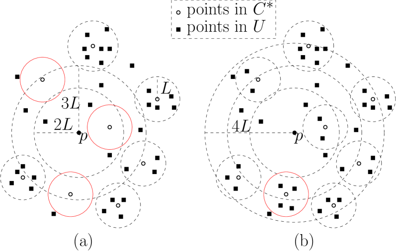
Figure 1: Two cases in proof of Lemma 2.3. In Figure (a), the balls ${\left\{{\mathsf{ball}}_{U}(c,L):c\in C^{*},d(p,c)\leq 3L\right\}}$ (red circles) are all empty. So, ${\mathsf{ball}}_{U}(p,2L)\subseteq O$. In Figure (b), there is a non-empty ${\mathsf{ball}}_{U}(c,L)$ for some $c\in C^{*}$ with $d(p,c)\leq 3L$ (the red circle). The ball is contained in ${\mathsf{ball}}_{U}(p,4L)$.

Figure 2: Illustration for proof of Lemma 2.7. $f_{i}:V_{i}\to P^{\prime}_{i}$ is indicated by the dashed lines, each of whom is of length at most $4L$. The number of crosses in a circle is at most $\frac{\epsilon z}{km}$.

2.2 The Main Algorithm

We are now ready to describe the main algorithm for the $(k,z)$-center problem, given in Algorithm 3. In the first round, each machine will call $\mathsf{aggregating}(P_{i},L,\frac{\epsilon z}{km})$ to obtain $(P^{\prime}_{i},w^{\prime}_{i})$. All the machines will first send their corresponding $|P^{\prime}_{i}|$ to the coordinator. In Round 2 the algorithm will check if $\sum_{i\in[m]}|P^{\prime}_{i}|$ is small or not. If yes, send a “Yes” message to all machines; otherwise return “No” and terminate the algorithm. In Round 3, if a machine $i$ received a “Yes” message from the coordinator, then it sends the dataset $P^{\prime}_{i}$ with the weight vector $w^{\prime}_{i}$ to the coordinator. Finally in Round 4, the coordinator collects all the weighted points $P^{\prime}=\operatorname*{\bigcup}_{i\in[m]}P^{\prime}_{i}$ and run $\mathsf{kzc}$ on these points.

Algorithm 3 $\mathsf{dist\mathchar 45\relax kzc}$

input on all parties: $n,k$, $z$, $m$, $L$, $\epsilon$
input on machine $i$: dataset $P_{i}$ with $|P_{i}|=n_{i}$
output: a set $C^{\prime}\subseteq P$ or “No” (which certifies $L^{*}>L$)

 

Round 1 on machine $i\in[m]$

1:  $(P^{\prime}_{i},w^{\prime}_{i})\leftarrow\mathsf{aggregating}(P_{i},L,\frac{\epsilon z}{km})$ 

2:  send $|P^{\prime}_{i}|$ to the coordinator 

 

Round 2 on the coordinator

1:  if $\sum_{i\in[m]}|P^{\prime}_{i}|>km(1+1/\epsilon)$ then return “No” else send “Yes” to each machine $i\in[m]$

 

Round 3 on machine $i\in[m]$

1:  Upon receiving of a “Yes” message from the coordinator, respond by sending $(P^{\prime}_{i},w^{\prime}_{i})$

 

Round 4 on the coordinator

1:  let $P^{\prime}\leftarrow\operatorname*{\bigcup}_{i=1}^{m}P^{\prime}_{i}$

2:  let $w^{\prime}$ be the function from $P^{\prime}$ to $\mathbb{Z}_{>0}$ obtained by merging $w^{\prime}_{1},w^{\prime}_{2},\cdots,w^{\prime}_{m}$ 

3:  let $z^{\prime}\leftarrow(1+\epsilon)z+w^{\prime}(P^{\prime})-n$ 

4:  if $z^{\prime}<0$ then return “No” else return $\mathsf{kzc}(k,z^{\prime},(P^{\prime},w^{\prime}),L^{\prime}=5L)$ 

An immediate observation about the algorithm is that its communication cost is small:

Claim 2.4.

The communication cost of $\mathsf{dist\mathchar 45\relax kzc}$ is $O(\frac{km}{\epsilon})$.

Proof.

The total communication cost of Round 1 and Round 2 is $O(m)$. We run Round 3 only when the coordinator sent the “Yes” message, in which case the communication cost is at most $\sum_{i=1}^{m}|P^{\prime}_{i}|\leq km(1+1/\epsilon)=O(\frac{km}{\epsilon})$. ∎

It is convenient to define some notations before we make further analysis. For every machine $i\in[m]$, let $P^{\prime}_{i}$ be the $P^{\prime}_{i}$ constructed in Round 1 on machine $i$. Let $V_{i}=\operatorname*{\bigcup}_{p\in P^{\prime}_{i}}{\mathsf{ball}}_{P_{i}}(p,4L)$ be the set of points in $P_{i}$ that are within distance at most $4L$ to some point in $P^{\prime}_{i}$. Notice that this is the definition of $V$ in Claim 2.2 for the execution of $\mathsf{aggregating}$ on machine $i$. Let $U_{i}=P_{i}\setminus V_{i}$; this is the set $U$ at the end of this execution. Let $f_{i}$ be the mapping from $V_{i}$ to $P^{\prime}_{i}$ satisfying Property 3 of Claim 2.2. Let $V=\operatorname*{\bigcup}_{i\in[m]}V_{i},P^{\prime}=\operatorname*{\bigcup}_{i\in[m]}P^{\prime}_{i}$ and $f$ be the function from $V$ to $P^{\prime}$, obtained by merging $f_{1},f_{2},\cdots,f_{m}$. Thus $(p,f(p))\leq 4L,\forall p\in V$ and $w^{\prime}(q)=|f^{-1}(q)|,\forall q\in P^{\prime}$.

Claim 2.5.

If $\mathsf{dist\mathchar 45\relax kzc}$ returns a set $C^{\prime}$, then $C^{\prime}$ is a $(k,(1+\epsilon)z)$-center solution to the instance $P$ with cost at most $24L$.

Proof.

$C^{\prime}$ must be returned in Step 4 in Round 4. By Theorem 2.1 for $\mathsf{kzc}$, $C^{\prime}$ is a $(k,z^{\prime})$-center solution to $(P^{\prime},w^{\prime})$ of cost at most $4\cdot 5L=20L$. That is, $w^{\prime}\left(P^{\prime}\setminus\operatorname*{\bigcup}_{c\in C^{\prime}}{\mathsf{ball}}_{P^{\prime}}(c,20L)\right)\leq z^{\prime}$. This implies $w^{\prime}\left(\operatorname*{\bigcup}_{c\in C^{\prime}}{\mathsf{ball}}_{P^{\prime}}(c,20L)\right)\geq w^{\prime}(P^{\prime})-z^{\prime}=n-(1+\epsilon)z$. Notice that for each $q\in P^{\prime}$, the set $f^{-1}(q)\subseteq V\subseteq P$ of points are within distance $4L$ from $q$ and $w^{\prime}(q)=|f^{-1}(q)|$. So, $\left|\operatorname*{\bigcup}_{c\in C^{\prime}}{\mathsf{ball}}_{P}(c,24L)\right|\geq n-(1+\epsilon)z$, which is exactly $\left|P\setminus\operatorname*{\bigcup}_{c\in C^{\prime}}{\mathsf{ball}}_{P}(c,24L)\right|\leq(1+\epsilon)z$. ∎

We can now assume $L\geq L^{*}$ and we need to prove that we must reach Step 4 in Round 4 and return a set $C^{\prime}$. We define $C^{*}\subseteq P$ to be a set of size $k$ such that $|P\setminus\operatorname*{\bigcup}_{c\in C^{*}}{\mathsf{ball}}(c,L)|\leq z$. Let $I=\operatorname*{\bigcup}_{c\in C^{*}}{\mathsf{ball}}_{P}(c,L)$ be the set of “inliers” according to $C^{*}$ and $O=P\setminus I$ be the set of outliers. Thus, $|I|\geq n-z$ and $|O|\leq z$.

Lemma 2.6.

After Round 1, we have $\sum_{i\in[m]}|P^{\prime}_{i}|\leq km(1+1/\epsilon)$.

Proof.

Let $z_{i}=|P_{i}\cap O|=\Big{|}P_{i}\setminus\operatorname*{\bigcup}_{c\in C^{*}}{\mathsf{ball}}_{P_{i}}(c,L)\Big{|}$ be the set of outliers in $P_{i}$. Then, $C^{*}$ is a $(k,z_{i})$-center solution to the instance $P_{i}$ with cost at most $L$. By Lemma 2.3, we have that $|P^{\prime}_{i}|\leq k+\frac{z_{i}}{\epsilon z/(km)}$. So, we have

$$\textstyle\sum_{i\in[m]}|P^{\prime}_{i}|\leq km+\frac{km}{\epsilon z}\sum_{i\in[m]}z_{i}\leq km\left(1+\frac{1}{\epsilon}\right).$$

Therefore, the coordinator will not return “No” in Round 2. It remains to prove the following Lemma.

Lemma 2.7.

Algorithm 3 will reach Step 4 in Round 4 and return a set $C^{\prime}$.

Proof.

See Figure 2 for the illustration of the proof. By Property 2 of Claim 2.2, we have $\left|{\mathsf{ball}}_{U_{i}}(p,2L)\right|\leq\frac{\epsilon z}{km}$ for every $p\in U_{i}$ since $U_{i}\subseteq P_{i}$. This implies that for every $c\in C^{*}$, we have $\left|{\mathsf{ball}}_{U_{i}}(c,L)\right|\leq\frac{\epsilon z}{km}$. (Otherwise, taking an arbitrary $p$ in the ball leads to a contradiction.)

$$\quad|U_{i}\cap I|=\Big{|}\operatorname*{\bigcup}_{c\in C^{*}}{\mathsf{ball}}_{U_{i}}(c,L)\Big{|}\leq\sum_{c\in C^{*}}|{\mathsf{ball}}_{U_{i}}(c,L)|\leq\sum_{c\in C^{*}}\frac{\epsilon z}{km}\leq\frac{\epsilon z}{m},\quad\forall i\in[m].$$

$$\quad\sum_{i\in[m]}|I\cap V_{i}|=\sum_{i\in[m]}\big{(}|I\cap P_{i}|-|I\cap U_{i}|\big{)}\geq\sum_{i\in[m]}\left(|I\cap P_{i}|-\frac{\epsilon z}{m}\right)=|I|-\epsilon z\geq n-(1+\epsilon)z.$$

For every $p\in V\cap I$, $f(p)$ will have distance at most $L+4L=5L$ to some center in $C^{*}$. Also, notice that $w^{\prime}(q)=|f^{-1}(q)|$ for every $q\in P^{\prime}$, we have that

$$\textstyle w^{\prime}\big{(}\operatorname*{\bigcup}_{c\in C^{*}}{\mathsf{ball}}_{P^{\prime}}(c,5L)\big{)}\geq|V\cap I|\geq n-(1+\epsilon)z.$$

So, $w^{\prime}(P^{\prime}\setminus\operatorname*{\bigcup}_{c\in C^{*}}{\mathsf{ball}}_{P^{\prime}}(c,5L))\leq w(P^{\prime})-n+(1+\epsilon)z=z^{\prime}$. This implies that $z^{\prime}\geq 0$, and there is a $(k,z^{\prime})$-center solution $C^{*}\subseteq P$ to the instance $(P^{\prime},w^{\prime})$ of cost at most $5L$. Thus $\mathsf{dist\mathchar 45\relax kzc}$ will reach Step 4 in Round 4 and returns a set $C^{\prime}$. This finishes the proof of the Lemma. ∎

We now briefly analyze the running times of algorithms on all parties. The running time of computing $P^{\prime}_{i}$ on each machine $i$ in round 1 is $O(n_{i}^{2})$ and this is the bottleneck for machine $i$. Considering all possible values of $L$, the running time on machine $i$ is $O\left(n_{i}^{2}\cdot\frac{\log\Delta}{\epsilon}\right)$. The running time of the round-4 algorithm of the central coordinator for one $L$ will be $O\left(\left(\frac{km}{\epsilon}\right)^{2}\right)$. We sort all the interesting $L$ values in increasing order. The trick here is to run only the first two rounds of the main algorithm. The central coordinator then use binary search to find the smallest $L^{\prime}$ that the main algorithm sends out “Yes” in Round 2. And it proceeds to Round 3 and 4 only for this single $L^{\prime}$. So, the running time of the central coordinator can be made $O\left(\left(\frac{km}{\epsilon}\right)^{2}\right)$.

The quadratic dependence of running time of machine $i$ on $n_{i}$ might be an issue when $n_{i}$ is big; we discuss how to alleviate the issue in the supplementary material.

3 Conclusion

In this paper, we give a distributed $(24(1+\epsilon),1+\epsilon)$-bicriteria approximation for the $(k,z)$-center problem, with communication cost $O\left(\frac{km}{\epsilon}+\frac{m\log\Delta}{\epsilon}\right)$. The running times of the algorithms for all parties are polynomial. We evaluate the algorithm on realworld data sets and it outperforms most previous algorithms, matching the performance of the state-of-art method[12].

For the $(k,z)$-median/means problem, we give a distributed $(1+\epsilon,1+\epsilon)$-bicriteria approximation algorithm with communication cost $O\left(\Phi D\cdot\frac{\log\Delta}{\epsilon}\right)$, where $\Phi$ is the upper bound on the size of the coreset constructed using the algorithm of [3]. The central coordinator needs to solve the optimization problem of finding a solution that is simultaneously good for $O\left(\frac{\log(\Delta n/\epsilon)}{\epsilon}\right)$ $k$-median/means instances. Since the approximation ratio for this problem will go to both factors in the bicriteria ratio, we really need a $(1+\epsilon)$-approximation for the optimization problem. Unfortunately, solving $k$-median/means alone is already APX-hard, and we don’t know a heuristic algorithm that works well in practice (e.g, a counterpart to Lloyd’s algorithm for $k$-means). It is interesting to study if a different approach can lead to a polynomial time distributed algorithm with $O(1)$-approximation guarantee.

Appendix A Necessity of Linear Dependence of Communication Cost on $z$ for True Approximation Algorithms

In this section, we show that if one is aiming for a multiplicative approximation for the $(k,z)$-center, $(k,z)$-median, or $(k,z)$-means problem, then the communication cost is at least $\Omega(z)$ bits, even if there are only 2 machines. We show that deciding whether the optimum $(k,z)$-center solution has cost $0$ or not requires $\Omega(z)$ bits of communication. This holds for any combination of values for $n,k$ and $z$ such that $k+z\leq n-1$. Let $B=1$. The points are all in the real line $\mathbb{R}$. On machine 1, there are $n-z-2$ copies of points from the set ${\left\{-1,-2,\cdots,-(k-1)\right\}}$, where each one of the $k-1$ points appears either ${\left\lfloor\frac{n-z-2}{k-1}\right\rfloor}$ or ${\left\lceil\frac{n-z-2}{k-1}\right\rceil}$ times. Notice that each point in the set appears at least once in the set. Meanwhile, machine 1 has a set $A$ of different points in $[2(z+2)]$, and machine 2 has a set $B$ of different points in $[2(z+2)]$, and we have $|A|+|B|=z+2$. If $A\cap B\neq\emptyset$, then the cost of the optimum solution is 0. Let $e\in A\cap B$, then we can discard all points except $e$ from $A$ and $B$. Then we discarded exactly $z$ points and the remaining set of points are at $k-1+1=k$ locations. On the other hand, if $A\cap B=\emptyset$, then the cost of the optimum solution is not 0. Thus deciding whether the cost is 0 or not requires us to decide if $A\cap B=\emptyset$, which is exactly the set disjointness problem. This requires a communication cost of $\Omega(z)$ between machine 1 and machine 2.

Appendix B Dealing with Various Issues of the Algorithm for $(k,z)$-Center

In this section, we show how to handle various issues that our $(k,z)$-center algorithm might face.

When $d_{\min}$ and $d_{\max}$ are not given. We can remove the assumption that $d_{\min}$ and $d_{\max}$ are given to us. Let $d_{\min,i}$ and $d_{\max,i}$ be the minimum and maximum non-zero pairwise distances between points in $P_{i}$. The crucial observation is that running aggregating on $P_{i}$ for $L<d_{\min,i}$ is the same as running it for $L=0$, and running it for $L>d_{\max,i}$ is the same as running it for $L=d_{\max,i}$. Thus, machine $i$ only needs to consider $L$ values that are integer powers of $1+\epsilon$ inside $[d_{\min,i},(1+\epsilon)d_{\max,i})$, or $0$, and send results for these $L$ values. Since $d_{\min,i}\geq d_{\min}$ and $d_{\max,i}\geq l_{\max}$, the number of such $L$ values is at most $O\left(\frac{\log\Delta}{\epsilon}\right)$. Also notice that the data points sent from machine $i$ to the coordinator are all generated from $P_{i}$. Thus, the aspect ratio for the union of all points received by the coordinator, is at most $\Delta$. This can guarantee that the coordinator only needs to use $O(\log\frac{\log\Delta}{\epsilon})$ iterations in the binary search step in Round 4.

When $\Delta$ is super big. There are many ways to handle the case when $\Delta$ is super-large. In many applications, we know the nature of the dataset and have a reasonable guess on $L^{*}$. In other applications, we may be only interested in the case where $L^{*}\in[A,B]$: we are happy with any clustering of cost less than $A$ and any clustering of cost more than $B$ is meaningless. In these applications where we have inside information about the dataset, the number of guesses can be much smaller. Finally, if we allow more rounds in our algorithm, we can use binary search for the whole algorithm $\mathsf{dist\mathchar 45\relax kzc}$, not just inside Round 4. We only need to run the algorithm for $O\left(\log\frac{\log\Delta}{\epsilon}\right)$ iterations; this will increase the number of rounds to $O\left(\log\frac{\log\Delta}{\epsilon}\right)$, but decrease the communication cost to $O\left(\frac{km}{\epsilon}+m\log\frac{\log\Delta}{\epsilon}\right)$.

Handling the Quadratic Running Time of Round 1 on Machine $i$. In Round 1 of the algorithm $\mathsf{dist\mathchar 45\relax kzc}$, each machine $i$ needs to run $\mathsf{aggregating}$ on $n_{i}=|P_{i}|$ points, leading to a running time of order $O(n_{i}^{2})$. In cases where $n_{i}$ is large, the algorithm might be slow. We can decrease the running time, at the price of increasing the communication cost and the running time on the coordinator. We view each $i\in[m]$ as a collection of $t_{i}\geq 1$ sub-machines, for some integer $t_{i}\in[1,n_{i}]$. Then, we run $\mathsf{dist\mathchar 45\relax kzc}$ on the set of $\sum_{i\in[m]}t_{i}$ sub-machines, instead of the original set of $m$ machines. The communication cost of the algorithm $\mathsf{dist\mathchar 45\relax kzc}$ increases to $O\left(\frac{k\sum_{i\in[m]}t_{i}}{\epsilon}\cdot\frac{\log\Delta}{\epsilon}\right)$, and the running time on each machine $i$ decreases to $O\left(\frac{n_{i}}{t_{i}})^{2}\cdot t_{i}\cdot\frac{\log\Delta}{\epsilon}\right)=O\left(\frac{n_{i}^{2}}{t_{i}}\cdot\frac{\log\Delta}{\epsilon}\right)$, and the running time of the algorithm for the coordinator becomes $O\left(\left(\frac{k\sum_{i\in[m]}t_{i}}{\epsilon}\right)^{2}\cdot\log\frac{\log\Delta}{\epsilon}\right)$. Each machine $i$ can choose a $t_{i}$ so that the $O\left(\frac{n_{i}^{2}}{t_{i}}\cdot\frac{\log\Delta}{\epsilon}\right)$-time algorithm of Round 1 terminates in acceptable amount of time.

Appendix C Distributed Algorithms $(k,z)$-Median/Means

In this section, we give our distributed algorithm for the $(k,z)$-median/means problems in Euclidean metrics. Let $m,k,z,\epsilon,n,P\subseteq\mathbb{R}^{D}$ and ${\left\{P_{i}\right\}}_{i\in[m]}$ be as defined in the problem setting. Let $\delta>0$ be the confidence parameter; i.e, our algorithm needs to succeed with probability $1-\delta$. Also, we define a parameter $\ell\in\{1,2\}$ to indicate whether the problem we are considering is $(k,z)$-median ($\ell=1$) or $(k,z)$-means ($\ell=2$).

Recall that $d_{\min}$ and $d_{\max}$ are respectively the minimum and maximum non-zero pairwise distance between points in $P$. It is not hard to see that the optimum solution to the instance has cost either $0$ or at least $d^{\ell}_{\min}/\ell$. For a technical reason, we can redefine $d(p,q)$ as follows for every $p,q\in\mathbb{R}^{D}$:

$$d(p,q)=\begin{cases}0&\text{ if }\|p-q\|_{2}=0\\ \min\Big{\{}\max\{\|p-q\|,\epsilon d_{\min}/(2n)\},2d_{\max}\Big{\}}&\text{ otherwise}\end{cases}.$$

That is, we truncate distances below at $\epsilon d_{\min}/(2n)$, and above at $2d_{\max}$. It is easy to see that the problem w.r.t the new metric is equivalent to the original one up to a multiplicative factor of $1+\epsilon$. In the new instance, we have either $d(p,q)=0$ or $d(p,q)\in[\epsilon d_{\min}/(2n),2d_{\max}]$.

Given an integer $z^{\prime}\in[0,n)$ and a set $C$ of $k$ centers, we define

$$\mathsf{cost}_{z^{\prime}}(C):=\min_{P^{\prime}\subseteq P:|P^{\prime}|=n-z^{\prime}}\sum_{p\in P^{\prime}}d^{\ell}(p,C)$$

to be the cost of the solution $C$ to the $(k,z)$-median/mean instance defined by $P,d$ and $z^{\prime}$. In the above definition, we remove $z^{\prime}$ outliers and consider the cost incurred by the $n-z^{\prime}$ non-outliers. Notice the set $P^{\prime}$ that minimizes the cost is the set of $n-z^{\prime}$ points in $P$ that are closest to $C$.

For some technical reason, we need to allow $z^{\prime}$ to take real values in $[0,n)$. In this case, we define

$$\mathsf{cost}_{z^{\prime}}(C):=\min_{w^{\prime}\in[0,1]^{P}:w^{\prime}(P)=n-z^{\prime}}\sum_{p\in P}w^{\prime}_{p}d^{\ell}(p,C).$$

Given a set $C$ of $k$ centers, the optimum $w^{\prime}$ can be obtained in a greedy manner: assign 1 to the $n-{\left\lceil z^{\prime}\right\rceil}$ points in $P$ that are closest to $C$, assign ${\left\lceil z^{\prime}\right\rceil}-z^{\prime}$ to the point in $P$ that is the $n-{\left\lceil z^{\prime}\right\rceil}+1$-th closest to $C$, and assign $0$ to the remaining points.

C.1 The $(k,z)$-Median/Means Problem Reformulated

In this section, we reformulate the $(k,z)$-median/means problems in a way that will be useful for our algorithm design. Given a threshold $L\geq 0$, we define $d_{L}(p,q)=\min\{d(p,q),L\}$ for every two points $p,q\in\mathbb{R}^{D}$. In other words, $d_{L}$ is the metric $d$ with distances truncated at $L$. The following crucial lemma gives the reformulations of $k$-median/means problems:

Lemma C.1.

For any real number $z^{\prime}\in[0,n)$, and any set $C$ of $k$ centers, we have

$$\mathsf{cost}_{z^{\prime}}(C)=\sup_{L\geq 0}\big{(}\sum_{p\in P}d^{\ell}_{L}(p,C)-z^{\prime}L^{\ell}\big{)}.$$ (1)

Moreover, the superior is achieved when $L$ is the $(n-{\left\lfloor z^{\prime}\right\rfloor})$-th smallest number in the multi-set ${\left\{d(p,C):p\in P\right\}}$.

Proof.

Let $\bar{L}$ be the $(n-{\left\lfloor z^{\prime}\right\rfloor})$-th smallest number in the multi-set ${\left\{d(p,C):p\in P\right\}}$. Then it can be seen that $\mathsf{cost}_{z^{\prime}}(C)=\sum_{p\in P}d^{\ell}_{\bar{L}}(p,C)-z^{\prime}{\bar{L}}^{\ell}$. Indeed, $\mathsf{cost}_{z^{\prime}}(C)$ is the sum of the $n-z^{\prime}$ smallest numbers in $S:=\{d^{\ell}(p,C):p\in P\}$. (When $n-z^{\prime}$ is not an integer, then we take a fraction of the last number.) To compute the quantity on the right side, we truncate the numbers in $S$ at $\bar{L}^{\ell}$, and then take the sum of the truncated numbers minus $z^{\prime}\bar{L}^{\ell}$. Since $\bar{L}^{\ell}$ is the $(n-{\left\lfloor z^{\prime}\right\rfloor})$-th smallest number in $S$, this quantity is exactly $\mathsf{cost}_{z^{\prime}}(C)$.

It remains to prove that $\sum_{p\in P}d^{\ell}_{L}(p,C)-z^{\prime}L^{\ell}$ attains its maximum value at $L={\bar{L}}$. First consider any $L<{\bar{L}}$, and define $P^{\prime}={\left\{p\in P|L<d(p,C)<{\bar{L}}\right\}}$, and $P^{\prime\prime}={\left\{p\in P:d(p,C)\geq\bar{L}\right\}}$. By the definition of $\bar{L}$, we have $|P^{\prime\prime}|\geq{\left\lfloor z^{\prime}\right\rfloor}+1>z^{\prime}$. Then, we have

$$\left(\sum_{p\in P}d^{\ell}_{\bar{L}}(p,C)-z^{\prime}{\bar{L}}^{\ell}\right)-\left(\sum_{p\in P}d^{\ell}_{L}(p,C)-z^{\prime}L^{\ell}\right)$$

$$=\sum_{p\in P^{\prime}}(d^{\ell}(p,C)-L^{\ell})+|P^{\prime\prime}|(\bar{L}^{\ell}-L^{\ell})-z^{\prime}(\bar{L}^{\ell}-L^{\ell})\geq\sum_{p\in P^{\prime}}(d^{\ell}(p,C)-L^{\ell})\geq 0.$$

Now consider any $L>{\bar{L}}$ and define $P^{\prime}={\left\{p\in P:\bar{L}<d(p,C)<L\right\}}$ and $P^{\prime\prime}={\left\{p\in P:d(p,C)\geq L\right\}}$. By the definition of $\bar{L}$, we have $|P^{\prime}\cup P^{\prime\prime}|=\big{|}{\left\{p\in P:d(p,C)>\bar{L}\right\}}\big{|}\leq{\left\lfloor z^{\prime}\right\rfloor}\leq z^{\prime}$. Then, we have

$$\left(\sum_{p\in P}d_{\bar{L}^{\ell}}(p,C)-z^{\prime}{\bar{L}}^{\ell}\right)-\left(\sum_{p\in P}d^{\ell}_{L}(p,C)-z^{\prime}L^{\ell}\right)$$

$$=-\sum_{p\in P^{\prime}}(d^{\ell}(p,C)-\bar{L}^{\ell})-|P^{\prime\prime}|(L^{\ell}-\bar{L}^{\ell})+z^{\prime}(L^{\ell}-\bar{L}^{\ell})$$

$$\geq-|P^{\prime}|(L^{\ell}-\bar{L}^{\ell})-|P^{\prime\prime}|(L^{\ell}-\bar{L}^{\ell})+z^{\prime}(L^{\ell}-\bar{L}^{\ell})\geq 0.$$

This finishes the proof of the lemma. ∎

With the above lemma, the $(k,z)$-median/means problem becomes finding a set of $k$ centers $C\subseteq\mathbb{R}^{D}$ so as to minimize $\sup_{L\geq 0}\,(\sum_{p\in P}d^{\ell}_{L}(p,C)-zL^{\ell})$. To get a handle on the problem, we first discretize the value space for $L$. Formally, we only allow $L$ to take values in

$$\mathbb{L}:=\{0\}\cup\Big{(}{\left\{(1+\epsilon)^{t}:t\in\mathbb{Z}\right\}}\cap(\epsilon d_{\min}/(2(1+\epsilon)n),2d_{\max}]\Big{)}.$$

Then, we have $|\mathbb{L}|=O\left(\frac{\log(\Delta n/\epsilon)}{\epsilon}\right)$. We define $\mathsf{cost}^{\prime}_{z^{\prime}}(C)$ as in (1), except that we only consider $L$ values in $\mathbb{L}$. That is, for every $z^{\prime}\in[0,n)$ and a set $C$ of $k$ centers, we define

$$\mathsf{cost}^{\prime}_{z^{\prime}}(C):=\sup_{L\in\mathbb{L}}\left(\sum_{p\in P}d^{\ell}_{L}(p,C)-z^{\prime}L^{\ell}\right).$$ (2)

For a fixed $z^{\prime}$ and $C$, we have $\mathsf{cost}^{\prime}_{z^{\prime}}(C)\leq\mathsf{cost}_{z^{\prime}}(C)$, since the supreme is taken over a subset of $L$ values in the definition of $\mathsf{cost}^{\prime}_{z^{\prime}}(C)$. Now we show the other direction of the inequality:

Lemma C.2.

For every set $C$ of $k$ centers, and any $z^{\prime}\in[0,n]$, we have

$$\mathsf{cost}_{(1+\epsilon)^{\ell}z^{\prime}}(C)\leq(1+\epsilon)^{\ell}\mathsf{cost}^{\prime}_{z^{\prime}}(C).$$ (3)

Proof.

By Lemma C.1, we have that $\mathsf{cost}_{(1+\epsilon)^{\ell}{z^{\prime}}}(C)=\sup_{L\geq 0}\left(\sum_{p\in P}d^{\ell}_{L}(p,C)-(1+\epsilon)^{\ell}{z^{\prime}}L^{\ell}\right)$. Let $\bar{L}$ be the $L\in\mathbb{R}$ that achieves the maximum value. Thus, $\mathsf{cost}_{(1+\epsilon)^{\ell}{z^{\prime}}}(C)=\sum_{p\in P}d^{\ell}_{\bar{L}}(p,C)-(1+\epsilon)^{\ell}{z^{\prime}}\bar{L}^{\ell}$. By Lemma C.1 and the new definition of the metric $d$, we have $\bar{L}=0$ or $\bar{L}\in[\epsilon d_{\min}/(2n),2d_{\max}]$. Thus there is always a $L^{\prime}\in\mathbb{L}$ such that $\bar{L}\in[L^{\prime},(1+\epsilon)L^{\prime})$.

$$\mathsf{cost}_{(1+\epsilon)^{\ell}{z^{\prime}}}(C) =\sum_{p\in P}d^{\ell}_{\bar{L}}(p,C)-(1+\epsilon)^{\ell}{z^{\prime}}\bar{L}^{\ell}$$

$$\leq(1+\epsilon)^{\ell}\sum_{p\in P}d^{\ell}_{L^{\prime}}(p,C)-(1+\epsilon)^{\ell}{z^{\prime}}L^{\prime\ell}\leq(1+\epsilon)^{\ell}\mathsf{cost}^{\prime}_{{z^{\prime}}}(C).$$

The first inequality is by $L^{\prime}\leq\bar{L}<(1+\epsilon)L^{\prime}$ and the second inequality is by the definition of $\mathsf{cost}^{\prime}_{z^{\prime}}(C)$ and the fact that $L^{\prime}\in\mathbb{L}$. ∎

The lemma allows us to focus on the new objective function $\mathsf{cost}^{\prime}_{\tilde{z}}(C)$ for some suitably defined $\tilde{z}$.

C.2 Distributed Algorithm for the Reformulated Problem via $\epsilon$-Coresets

An important notion that has been used to design efficient algorithms for $k$-median/means in Euclidean space is the $\epsilon$-coreset. Roughly speaking, it is a weighted set of points that approximates the given set $P$ well. Formally,

Definition C.3.

A weighted set $(Q,w)$ of points is an $\epsilon$-coreset for $P^{\prime}$ w.r.t. distance $d^{\prime}$, if for every set $C\subseteq\mathbb{R}^{D}$ of $k$ centers, we have

$$\left(\sum_{q\in Q}w_{q}d^{\prime\ell}(q,C)\right)\Big{/}\left(\sum_{p\in P^{\prime}}d^{\prime\ell}(p,C)\right)\in[1-\epsilon,1+\epsilon].$$

The following theorem from [3] gives a distributed algorithm to construct $\epsilon$-coresets for the points $P$ and a truncated metric $d_{L}$:

Theorem C.4.

[3] Given $\delta>0,\epsilon>0,L\geq 0$, there is an $2$-round distributed algorithm that outputs an $\epsilon$-coreset $(Q,w)$ of $P$ w.r.t distance $d^{L}$, with probability at least $1-\delta$. The size of the coreset is at most $\Phi$, where $\Phi=O\left(\frac{1}{\epsilon^{2}}(kD+\log\frac{1}{\delta})+mk\right)$ for $k$-median, and $\Phi=O\left(\frac{1}{\epsilon^{4}}(kD+\log\frac{1}{\delta})+mk\log\frac{mk}{\delta}\right)$ for $k$-means. The communication complexity of the algorithm is $O(D\Phi)$.

The correspondent theorem in [3] only considers the original Euclidean metric $\|\cdot-\cdot\|_{2}$. In our definition of $d_{L}$, we truncated distances below at $\epsilon\cdot d_{\min}/(2n)$, and then above at $L$. But it is easy to extend their theorem so that it works for the truncated metrics, since all we need is that the metric has $O(D)$ “pseudo-dimension” (defined in [3]). Truncating the metric only change the pseudo-dimension by an additive constant. From now on, let $\Phi$ be the upper bound on the size of the $\epsilon$-coreset in Theorem C.4.

With Theorem C.4 in hand, it is straightforward to give our algorithm for $(k,z)$-median/means. For all $L\in\mathbb{L}$, we run in parallel the 2-round distributed algorithm in Theorem C.4 with $\delta$ scaled down by a factor of $|\mathbb{L}|$ to obtain a $\epsilon$-coreset $(Q_{L},w_{L})$. The communication cost of the algorithm is then $\Phi D\cdot\frac{\log(n\Delta/\epsilon)}{\epsilon}$.

Let $\tilde{z}=\frac{(1+\epsilon)^{2}z}{1-\epsilon}$. We would like to find a set $\tilde{C}$ of $k$ points that minimizes $\sup_{L\in\mathbb{L}}\left(\frac{1}{1-\epsilon}\sum_{q\in Q_{L}}w_{q}d^{\ell}_{L}(q,\tilde{C})-\tilde{z}L^{\ell}\right)$. However, it is not even clear whether the optimum $\tilde{C}$ can be represented using finite number of bits or not. Instead, the coordinator will output a set $\tilde{C}\subseteq\mathbb{R}^{D}$ of $k$ centers such that for every set $C^{*}\subseteq\mathbb{R}^{D}$ of $k$ centers, we have

$$\sup_{L\in\mathbb{L}}\left(\frac{1}{1-\epsilon}\sum_{q\in Q_{L}}w_{q}d^{\ell}_{L}(q,{\tilde{C}})-\tilde{z}L^{\ell}\right)\leq\sup_{L\in\mathbb{L}}\left(\frac{1+\epsilon}{1-\epsilon}\sum_{q\in Q_{L}}w_{q}d^{\ell}_{L}(q,C^{*})-\tilde{z}L^{\ell}\right).$$ (4)

The extra $(1+\epsilon)$ factor on the right-side allows us to partition the Euclidean space into finite number of cells. This can be done by partitioning the space into $O\left(\frac{\log(\Delta n/\epsilon)}{\epsilon}\right)^{|\mathbb{L}|\Phi}$ cells so that all points in a cell have similar respective distances to all points in $\operatorname*{\bigcup}_{L\in\mathbb{L}}Q_{L}$. So, we can choose an arbitrary representative point from each cell, and then enumerate all sets $\tilde{C}$ of $k$ representatives and output the one with the minimum $\sup_{L\in\mathbb{L}}\left(\frac{1}{1-\epsilon}\sum_{q\in Q_{L}}w_{q}d^{\ell}_{L}(q,{\tilde{C}})-\tilde{z}L^{\ell}\right)$. The running time of the algorithm can be bounded by $\exp\left(\Phi,k,|\mathbb{L}|,D,\log\left(\frac{\log(n\Delta/\epsilon)}{\epsilon}\right)\right)=\exp\left(\mathrm{poly}\left(\frac{1}{\epsilon},k,D,m,\log\frac{1}{\delta},\log\Delta\right)\right)$.

C.3 Analysis of the algorithm

We now show that the algorithm gives a $(1+O(\epsilon),1+O(\epsilon))$-approximation algorithm to the $(k,z)$-median/means problem. With probability at least $1-\delta$, for every $L$, the weighted set $(Q_{L},w_{L})$ is an $\epsilon$-corset for $P$ w.r.t metric $d_{L}$. Let $C^{*}$ be the optimal set of centers for the original $(k,z)$-median/means problem. Then, for every $z^{\prime}\in[0,n]$, we have

$$\quad\mathsf{cost}^{\prime}_{\tilde{z}}({\tilde{C}})$$

$$=\ \sup_{L\in\mathbb{L}}\left(\sum_{p\in P}d^{\ell}_{L}(p,{\tilde{C}})-\tilde{z}L^{\ell}\right) \ \leq\ \sup_{L\in\mathbb{L}}\left(\frac{1}{1-\epsilon}\sum_{q\in Q_{L}}w_{q}d^{\ell}_{L}(q,{\tilde{C}})-\tilde{z}L^{\ell}\right)$$

$$\leq\ \sup_{L\in\mathbb{L}}\left(\frac{1+\epsilon}{1-\epsilon}\sum_{q\in Q_{L}}w_{q}d^{\ell}_{L}(q,C^{*})-\tilde{z}L^{\ell}\right) \ \leq\ \sup_{L\in\mathbb{L}}\left(\frac{(1+\epsilon)^{2}}{1-\epsilon}\sum_{p\in P}d^{\ell}_{L}(p,C^{*})-\tilde{z}L^{\ell}\right)$$

$$=\ \frac{(1+\epsilon)^{2}}{1-\epsilon}\sup_{L\in\mathbb{L}}\left(\sum_{p\in P}d^{\ell}_{L}(p,C^{*})-zL^{\ell}\right) \ =\ \frac{(1+\epsilon)^{2}}{1-\epsilon}\mathsf{cost}^{\prime}_{z}(C^{*}).$$

The first and the third inequalities are by the definition of $\epsilon$-coreset, while the second inequality is by (4). Then with Lemma C.2, we know that

$$\mathsf{cost}_{\frac{(1+\epsilon)^{\ell+2}}{1-\epsilon}z}(\tilde{C}) =\mathsf{cost}_{(1+\epsilon)^{\ell}\tilde{z}}({\tilde{C}})\leq(1+\epsilon)^{\ell}\mathsf{cost}^{\prime}_{\tilde{z}}({\tilde{C}})$$

$$\leq\frac{(1+\epsilon)^{\ell+2}}{1-\epsilon}\mathsf{cost}^{\prime}_{z}(C^{*})\leq\frac{(1+\epsilon)^{\ell+2}}{1-\epsilon}\mathsf{cost}_{z}(C^{*}).$$

So, ${\tilde{C}}$ is a $\left(\frac{(1+\epsilon)^{\ell+2}}{1-\epsilon},\frac{(1+\epsilon)^{\ell+2}}{1-\epsilon}\right)=(1+O(\epsilon),1+O(\epsilon))$-approximate solution. We can scale down the input $\epsilon$ by a constant factor to obtain a $(1+\epsilon,1+\epsilon)$-approximation.

As we mentioned, the running time of the algorithm for the central coordinator is exponential in $\frac{1}{\epsilon},k,D,m,\log\frac{1}{\delta}$ and $\log\Delta$. For each machine $i$, the running time in the algorithm of [3] is dominated by the time to compute an $O(1)$-approximation for the $k$-median/$k$-means problem for $P_{i}$, which is polynomial in $n_{i}$ and $D$.

Appendix D Complete Experiment Results

D.1 $k$-Center Clustering with Outliers

We evaluate the performance of our $(k,z)$-center algorithm (Algorithm 3) on several real-world datasets, which are summarized in Table 1. In the experiments we compare $\mathsf{dist\mathchar 45\relax kzc}$ with many other $k$-center methods, including two centralized methods (greedy [15] and $\mathsf{kzc}$ [5] and four distributed methods (random-random, random-kzc, MKCWM [20], and GLZ [12]). The greedy method has a 2-approximation ratio in the no-outlier scenario, but doesn’t take outliers into account. The random-random and random-kzc methods serves as two baselines: random-random randomly sample $k+z$ points on each machine, then further randomly choose $k$ points from the total $m(k+z)$ sampled points as final cluster centers; random-kzc is similar to random-random, except that it chooses the final $k$ centers by the $\mathsf{kzc}$ method. The MKCWM and GLZ are the state-of-art distributed $k$-center algorithms that handle outliers. For each parameter setting the experiment is repeated for 5 runs and the average result is reported. Note the three distributed baseline methods random-random, random-kzc, and MKCWM all have the same communication cost $md(k+z)$, while GLZ’s communication cost is $\tilde{O}(mk+m/\epsilon)$. All methods are implemented in Python and the experiments are conducted on a 2-core 2.7 GHz Intel Core i5 laptop.

Name	Size: $n$	Dimension: $B$
spambase	4,601	57
parkinsons	5,875	16
pendigits2	10,992	16
letter2	20,000	16
skin2	245,057	3
covertype2	581,012	10
gas2	928,991	10
power2	2,049,280	7

Table 1: Clustering datasets used for evaluation

The experiments consist of two parts: In the first part we compare our algorithms with the two centralized methods. This part is conducted only for the 4 smaller datasets (spambase, parkinsons, pendigits, and letter), on which centralized methods can finish in an acceptable time. In the second part we compare our algorithms with other distributed methods on the 4 larger datasets (skin, covertype, gas, and power).

Distributed v.s. Centralized: Figure 3 and Figure 4 show the results on the four smaller datasets. Figure 3 demonstrates how the objective value and communication cost change with $z$ when $k$ is fixed to $20$. Our algorithm $\mathsf{dist\mathchar 45\relax kzc}$ always achieve comparable objective with other distributed baselines. On datasets spambase and parkinsons, the objective value even matches the best centralized method ($\mathsf{kzc}$). When it comes to communication cost, $\mathsf{dist\mathchar 45\relax kzc}$ shows a clear advantage over random-random, random-kzc, and MKCWM, which matches our theoretical results.

Figure 4 depicts the performance with respect to different value of $k$ when $z$ is fixed to $256$. $\mathsf{dist\mathchar 45\relax kzc}$ still achieves similar (or better) objective values among all distributed methods. But we can see that when $k$ increases, the communication cost of $\mathsf{dist\mathchar 45\relax kzc}$ ($\epsilon=0.1$) approaches those of other distributed methods. Recall that the communication cost of $\mathsf{dist\mathchar 45\relax kzc}$ is $\tilde{O}(mk/\epsilon)$ which can be similar to $O(m(k+z))$ when $z$ and $k/\epsilon$ are in the same order. If we choose a large value of $\epsilon=0.99$, the communication cost of $\mathsf{dist\mathchar 45\relax kzc}$ becomes much stable, while the objective value is only slightly worse. This suggests that in practice we can choose a relatively large $\epsilon$ to obtain small communication cost.

We want to remind the readers that the approximation ratio of $\mathsf{dist\mathchar 45\relax kzc}$ holds for removing $(1+\epsilon)z$ outliers, while in the experiments the objective is computed by removing only $z$ outliers. This indicates that $\mathsf{dist\mathchar 45\relax kzc}$ may have better performance than what is predicted theoretically.

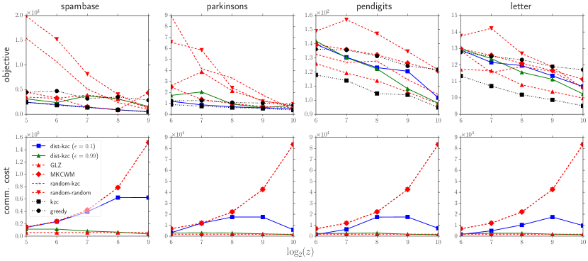
Figure 3: Centralized vs. Distributed, with varying $z$ and fixed $k=20,m=5$.

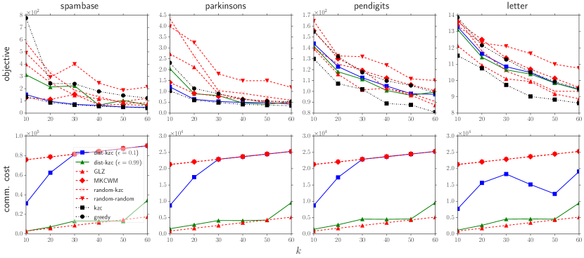
Figure 4: Centralized vs. Distributed, with varying $k$ and fixed $z=256,m=5$.

Large scale: This part contains experiment results on the four large datasets: skin, covertype, gas, and power. The GLZ method needs solving many local $(k,z^{\prime})$-center instances, which is too slow to finish on these large datasets. Hence here we use its variant provided by [12], denoted as GLZ-z. GLZ-z works similar as GLZ, but avoids solving $(k,z^{\prime})$-center locally on each machine by transmitting $\tilde{O}(mk+z)$ data to the coordinator. So GLZ-z has a higher communication cost than GLZ, but it’s still much better than MKCWM which has a $O(m(k+z))$ communication cost.

Similar to the previous part, Figure 5 and Figure 6 show results for varying $z$ and $k$. Our method still achieves comparable objective value with the best distributed baselines. The communication cost of our algorithm is always much smaller than MKCWM, and matches that of GLZ-z. This advantage is more obvious with bigger $z$, but here to make all the baselines terminate in acceptable times we only use $z\sim\sqrt{n}$.

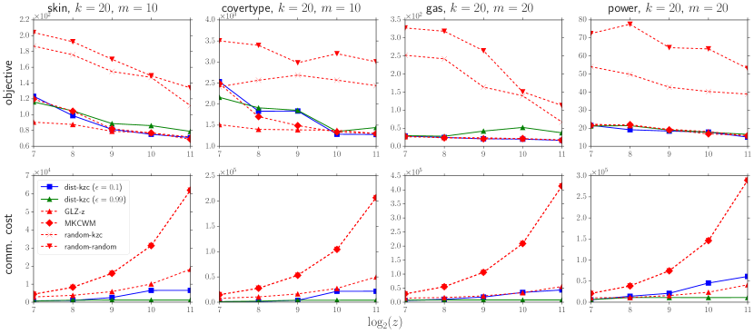
Figure 5: Large scale, with varying $z$

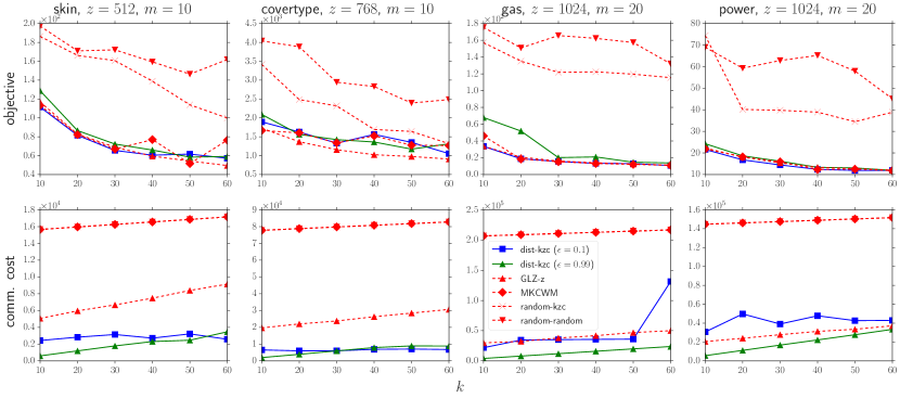
Figure 6: Large scale, with varying $k$

D.2 $k$-Means Clustering with Outliers

The centralized solver: We test our distributed $k$-means algorithm proposed in section C. As we described, the algorithm requires solving a min-max clustering problem on the coordinator. Formally, given a set of datasets $Q_{1},\ldots,Q_{M}$, each equipped with its own metric $d_{1},\ldots,d_{M}$, the goal is to find a center set $C$ minimizing the maximum cost over all $M$ datasets:

$$\min_{C:|C|=k}\max_{i\in[M]}\sum_{p\in Q_{i}}d^{l}_{i}(p,Q_{i})$$ (5)

where $l=1,2$ corresponding to the $k$-median or $k$-means objective respectively.

Although we don’t know any practical algorithm for such min-max clustering problem, there exists some results addressing a simpler form of the min-max $k$-median problem: Suppose there’re only $N$ possible locations for selecting the center set $F$ (i.e., $C\subset V$ for some $|V|=N$), and every dataset $Q_{i}$ has the same metric $d$, then Anthony et al. [2] shows that a simple reverse-greedy method achieves $O(\log N+\log M)$-approximation for the min-max $k$-median problem in this special case. We adapt their method to solve our min-max $k$-means problem in the experiment. For completeness, the algorithm is listed below:

Algorithm 4 reverse-greedy $(k,\{(Q_{i},d_{i})\}_{i=1}^{M},B)$[2]

1:  $C^{1}\leftarrow\bigcup_{i=1}^{M}Q_{i},w^{1}_{i}\longleftarrow 1$ for all $i\in[M]$;

2:  for $t\leftarrow 1$ to $N-k$ do

3:      For every $v\in F^{t}$ and $i\in[M]$, let $\delta^{t}_{i}(v)\leftarrow\sum_{p\in Q_{i}}(d^{2}_{i}(p,C^{t}\setminus\{v\})-d^{2}_{i}(p,C^{t}))$

4:      $\hat{C}^{t}\leftarrow\{v\in C^{t}|\forall i\in[M],\delta^{t}_{i}(v)\leq B/2\}$ 

5:      $v^{t}\leftarrow\operatorname*{arg\,min}_{v\in\hat{C}^{t}}\sum_{i=1}^{M}w^{t}_{i}\cdot\delta^{t}_{i}(v)$  

6:      For all $i\in[M]$, let $w^{t+1}_{i}\leftarrow w^{t}_{i}\left(1+\frac{1}{B}\right)^{\delta^{t}_{i}(v^{t})}$ 

7:  return $C^{N-k+1}$

Roughly speaking, the algorithm starts with $C$ being the set of all points, and iteratively remove points in $C$ until it shrinks to size $k$. In each iteration the algorithm removes from $C$ the point that incurs the least weighted total cost increase. However, because our problem is more general than that in [2], we don’t know whether their approximation guarantee for Algorithm 4 still holds here.

Algorithms: We compare our implementation with some other algorithms for the $k$-means/$(k,z)$-means problem, including two centralized ones and two distributed ones: k-means [19], the classical Lloyd’s algorithm; k-means$--$ [6], like k-means, but uses some heuristics to handle outliers; BEL [3], the distributed $k$-means algorithm based on coreset; and CAZ [7], a recently proposed distributed $(k,z)$-means algorithm. The BEL and CAZ algorithms both belong to the two-level clustering framework[13]: first construct a local summary on each machine and aggregate them on the coordinator, then the coordinator conduct a centralized clustering over the aggregated summaries to get the final result. But the main focus of BEL and CAZ is how to construct local summary, and they don’t specify the actual coordinator solver used. In the experiment we use k-means and k-means$--$ as the centralized solver for BEL and CAZ respectively. All methods are implemented in Python and the experiments are conducted on a 2-core 2.7 GHz Intel Core i5 laptop.

Datasets: The experiment is conducted on one synthesized dataset and three real-world datasets. The real-world datasets are spambase, parkinsons, and pendigits (see Table 1). Unlike the $k$-center case, the outliers in the original dataset are unable to significantly affect the objective value. Thus to make the algorithm’s effect clearer, we manually add 500 outlier points to each of the three dataset. The synthesized dataset is sampled from a mixture of Gaussian model, of which the parameters are also randomly generated; specifically, we sample 10000 points in total from 4 different Gaussian distributions in $\mathbb{R}^{5}$, and manually add another 500 outliers to the dataset.

Parameter setting: For each dataset, we fix $k$ and vary $z$. On the three real-world datasets, $k$ is set to be $10$ and $z$ varies from $2^{5}$ to $2^{11}$; on the synthesized dataset, $k$ is set to be $4$ and $z$ ranges from $2^{6}$ to $2^{10}$. The number of machines are fixed to $5$ for all 4 datasets. Throughout the experiment, we use $\epsilon=0.3$ as the error parameter for our algorithm. We measure how the objective value and communication cost (for distributed methods only) changes with $z$. But different from the setting in Section D.1, here we compute the cost of our method by removing $(1+\epsilon)z$ outliers to match our theory result. (In this sense, the comparison is “more fair” for us than in Section D.1)

Another issue in applying our $(k,z)$-means algorithm is the choice of appropriate coreset size. Unlike the result for our $(k,z)$-center algorithm, we only have an asymptotic estimation for the coreset size, which is not so instructive in practice. Therefore, in the experiment we hand-pick the coreset size by some heuristics: when the value of the error parameter $\epsilon$ is given, we can compute the total number of different threshold distance that will be tried (i.e., $|\mathbb{L}|$). Then we choose the coreset size to be $\max\left\{10k,\frac{n}{10m|\mathbb{L}|}\right\}$. So each coreset contains at least $10k$ samples, and when $n\gg km|\mathbb{L}|$, we allow the total size to be as large as $n/10$.

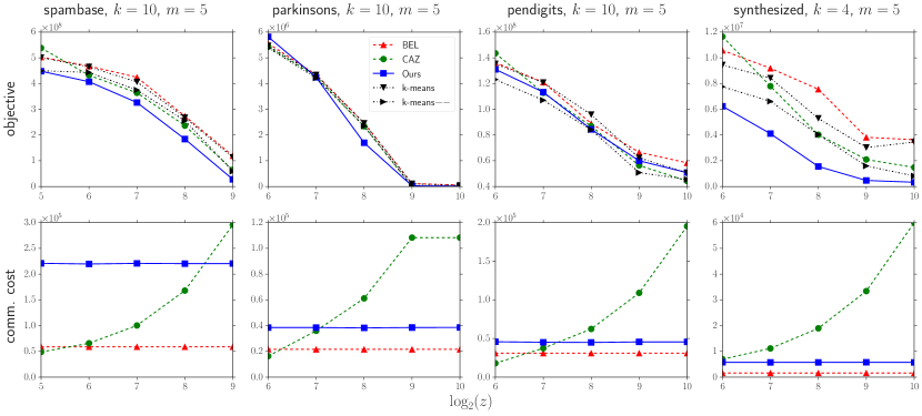
Figure 7: Comparison of the our distributed $(k,z)$-means implementation with other distributed/centralized methods. The first row is objective value, and the second is communication cost.

Experiment results: Figure 7 shows the experiment result: we can see that our algorithm performs surprisingly well in terms of objective value, often achieving the lowest cost among all the methods. The effect of outliers is most clearly revealed on the synthesized data, where BEL and k-means perform significantly worse than others. In particular, although we remove $\epsilon z$ more outliers when calculating the cost for our method, it’s still much better than BEL even if compared at different $z$: consider our method’s cost at $z=(1+\epsilon)2^{7}=1.3\cdot 2^{7}$ with BEL’s at $z=2^{8}$.

The communication cost of our method doesn’t change with $z$, since the way we decide the coreset size makes it fixed. BEL’s communication cost is also not affected by $z$, as it doesn’t deal with outliers. In contrast, CAZ’s communication is in the order of $O(mk\log n+z)$, which is reflected in the figure as it grows linearly in $z$. Although our centralized solver uses some heuristics and thus doesn’t have provable guarantees, the experiment results suggest that our coresets construction indeed preserves the outliers information while being independent of $z$.

References

- [1] Sara Ahmadian, Ashkan Norouzi-Fard, Ola Svensson, and Justin Ward. Better guarantees for k-means and euclidean k-median by primal-dual algorithms. In 58th IEEE Annual Symposium on Foundations of Computer Science, FOCS 2017, Berkeley, CA, USA, October 15-17, 2017, pages 61–72, 2017.
- [2] Barbara M. Anthony, Vineet Goyal, Anupam Gupta, and Viswanath Nagarajan. A plant location guide for the unsure: Approximation algorithms for min-max location problems. Math. Oper. Res., 35(1):79–101, 2010.
- [3] Maria-Florina Balcan, Steven Ehrlich, and Yingyu Liang. Distributed k-means and k-median clustering on general communication topologies. In Advances in Neural Information Processing Systems 26, NIPS 2013, December 5-8, 2013, Lake Tahoe, Nevada, United States., pages 1995–2003, 2013.
- [4] Jaroslaw Byrka, Thomas Pensyl, Bartosz Rybicki, Aravind Srinivasan, and Khoa Trinh. An improved approximation for k-median and positive correlation in budgeted optimization. ACM Trans. Algorithms, 13(2):23:1–23:31, 2017.
- [5] Moses Charikar, Samir Khuller, David M. Mount, and Giri Narasimhan. Algorithms for facility location problems with outliers. In Proceedings of the 12th Annual Symposium on Discrete Algorithms, January 7-9, 2001, Washington, DC, USA., pages 642–651, 2001.
- [6] Sanjay Chawla and Aristides Gionis. k-means: A unified approach to clustering and outlier detection. In Proceedings of the 13th SIAM International Conference on Data Mining, May 2-4, 2013. Austin, Texas, USA., pages 189–197, 2013.
- [7] Jiecao Chen, Erfan Sadeqi Azer, and Qin Zhang. A practical algorithm for distributed clustering and outlier detection. CoRR, abs/1805.09495, 2018.
- [8] Jiecao Chen, He Sun, David P. Woodruff, and Qin Zhang. Communication-optimal distributed clustering. In Advances in Neural Information Processing Systems 29: Annual Conference on Neural Information Processing Systems 2016, December 5-10, 2016, Barcelona, Spain, pages 3720–3728, 2016.
- [9] Ke Chen. A constant factor approximation algorithm for k-median clustering with outliers. In Proceedings of the 19th Annual ACM-SIAM Symposium on Discrete Algorithms, SODA 2008, San Francisco, California, USA, January 20-22, 2008, pages 826–835, 2008.
- [10] Hu Ding, Yu Liu, Lingxiao Huang, and Jian Li. -means clustering with distributed dimensions. In Proceedings of the 33rd International Conference on Machine Learning, ICML 2016, New York City, NY, USA, June 19-24, 2016, pages 1339–1348, 2016.
- [11] Alina Ene, Sungjin Im, and Benjamin Moseley. Fast clustering using mapreduce. In Proceedings of the 17th ACM SIGKDD International Conference on Knowledge Discovery and Data Mining, San Diego, CA, USA, August 21-24, 2011, pages 681–689, 2011.
- [12] Sudipto Guha, Yi Li, and Qin Zhang. Distributed partial clustering. In Proceedings of the 29th ACM Symposium on Parallelism in Algorithms and Architectures, SPAA 2017, Washington DC, USA, July 24-26, 2017, pages 143–152, 2017.
- [13] Sudipto Guha, Adam Meyerson, Nina Mishra, Rajeev Motwani, and Liadan O’Callaghan. Clustering data streams: Theory and practice. IEEE Trans. Knowl. Data Eng., 15(3):515–528, 2003.
- [14] Johan Håstad and Avi Wigderson. The randomized communication complexity of set disjointness. Theory of Computing, 3(1):211–219, 2007.
- [15] Dorit S. Hochbaum and David B. Shmoys. A best possible heuristic for the k-center problem. Math. Oper. Ues., 10(2):180–184, 1985.
- [16] Sungjin Im and Benjamin Moseley. Brief announcement: Fast and better distributed mapreduce algorithms for k-center clustering. In Proceedings of the 27th ACM on Symposium on Parallelism in Algorithms and Architectures, SPAA 2015, Portland, OR, USA, June 13-15, 2015, pages 65–67, 2015.
- [17] Ravishankar Krishnaswamy, Shi Li, and Sai Sandeep. Constant approximation for k-median and k-means with outliers via iterative rounding. In Proceedings of the 50th Annual ACM SIGACT Symposium on Theory of Computing, STOC 2018, Los Angeles, CA, USA, June 25-29, 2018, pages 646–659, 2018.
- [18] M. Lichman. UCI machine learning repository, 2013.
- [19] Stuart P. Lloyd. Least squares quantization in PCM. IEEE Trans. Information Theory, 28(2):129–136, 1982.
- [20] Gustavo Malkomes, Matt J. Kusner, Wenlin Chen, Kilian Q. Weinberger, and Benjamin Moseley. Fast distributed k-center clustering with outliers on massive data. In Advances in Neural Information Processing Systems 28, NIPS 2015, December 7-12, 2015, Montreal, Quebec, Canada, pages 1063–1071, 2015.
- [21] Athanasios Tsanas, Max A. Little, Patrick E. Mcsharry, and Lorraine O. Ramig. Enhanced classical dysphonia measures and sparse regression for telemonitoring of parkinson’s disease progression. In Proceedings of the IEEE International Conference on Acoustics, Speech, and Signal Processing, ICASSP 2010, 14-19 March 2010, Dallas, Texas, USA, pages 594–597, 2010.