Ring modes supported by concentrated cubic nonlinearity

Abstract

We consider the one-dimensional Schrödinger equation on a ring, with the cubic term, of either self-attractive or repulsive sign, confined to a narrow segment. This setting can be realized in optics and Bose-Einstein condensates. For the nonlinearity coefficient represented by the delta-function, all stationary states are obtained in an exact analytical form. The states with positive chemical potentials are found in alternating bands for the cases of the self-repulsion and attraction, while solutions with negative chemical potentials exist only in the latter case. These results provide a possibility to obtain exact solutions for bandgap states in the nonlinear system. Approximating the delta-function by a narrow Gaussian, stability of the stationary modes is addressed through numerical computation of eigenvalues for small perturbations, and verified by simulations of the perturbed evolution. For positive chemical potentials, the stability is investigated in three lowest bands. In the case of the self-attraction, each band contains a stable subband, the transition to instability occurring with the increase of the total norm. As a result, multi-peak states may be stable in higher bands. In the case of the self-repulsion, a single-peak ground state is stable in the first band, while the two higher ones are populated by weakly unstable two- and four-peak excited states. In the case of the self-attraction and negative chemical potentials, single-peak modes feature instability which transforms them into persistently oscillating states.

I Introduction and the model

The use of spatially modulated nonlinearities makes it possible to greatly expand varieties of solitons supported by competition of local nonlinearities and linear diffraction or dispersion FA ; PGK ; RMP . The simplest example of such settings is represented by a continuous linear medium into which a cubic self-focusing nonlinearity is embedded in a narrow region, that may be approximated by the coefficient in front of the cubic term taken as the delta-function, $\delta(x)$. This approximation leads to the following limit form of the nonlinear Schrödinger equation (NLSE) for wave function $\psi\left(x,t\right)$ [alias the Gross-Pitaevskii equation, in terms of atomic Bose-Einstein condensates (BECs) GPE ],

$$i\psi_{t}+\frac{1}{2}\psi_{xx}+\varepsilon\delta(x)|\psi|^{2}\psi=0,$$ (1)

written in the scaled form, with strength $\varepsilon>0$ of the self-focusing. This model was introduced in Ref. Mark , where the scattering problem for a plane wave hitting the localized nonlinearity was considered, and localized modulational instability of the solution to the scattering problem was discovered. Note that $\varepsilon$ may be fixed as an arbitrary positive value by means of obvious rescaling of wave function $\psi$.

In the application to optics, with time $t$ in Eq. (1) replaced by the propagation distance, $z$ KA , a narrow nonlinearity-bearing stripe embedded in a planar nonlinear waveguide may be created by implanting nonlinear dopants into the host linear medium Kip . In BEC, a similar effect can be achieved by the locally induced Feshbach resonance, controlled by a tightly focused laser beam, as suggested by the techniques demonstrated in Refs. Painting and FR1 -FR3 .

NLSE in the form of Eq. (1) gives rise to an obvious family of pinned modes (solitons), parameterized by chemical potential $\mu<0$,

$$\psi=\left(-2\mu\right)^{1/4}\exp\left(-i\mu t-\sqrt{-2\mu}|x|\right)$$ (2)

(in terms of the NLSE for the propagation of light in planar waveguides, $-\mu$ is the propagation constant). The norm of the solitons (alias the integral power of the optical beam),

$$N=\int_{-\infty}^{+\infty}\left|\psi(x)\right|^{2}dx,$$ (3)

is degenerate for family (2), taking a single value which does not depend on $\mu$, $N\equiv 1$. The norm degeneracy is a characteristic feature of families of Townes solitons (TS) Townes , which exist in models featuring the critical collapse driven by self-attractive nonlinearities Berge ; Fibich . Accordingly, this family formally seems neutrally stable in terms of the well-known Vakhitov-Kolokolov (VK) criterion, $dN/d\mu<0$, which often plays the role of the necessary stability criterion for self-trapped states maintained by attractive nonlinearities VK ; Berge ; Fibich . However, in reality solitons of the TS type are subject to nonlinear (subexponentially growing) instability, which destroys them Berge ; Fibich . Indeed, the soliton family (2) is completely unstable, in the framework of Eq. (1) Nir . It is relevant to mention that, while the original TS family is represented by axially symmetric solutions of the two-dimensional NLSE with the cubic nonlinearity Townes , a similar family is known in one dimension too, in the form of the NLSE with the quintic self-focusing 1DTownes . In fact, the soliton family (2) may be considered as an alternative example of the TS family in one dimension.

Because below we also consider the model with the repulsive localized nonlinearity, $\varepsilon<0$ in Eq. (4), it is relevant to mention that, in cases when the repulsive nonlinearity may support self-trapped modes (e.g., gap solitons, in the presence of a spatially periodic potential gap1 -gap3 ), their necessary stability condition may amount to the anti-VK criterion, $dN/d\mu>0$ HS . Note that the localized repulsive nonlinear term can be efficiently used as a splitter in the design of soliton-based matter-wave interferometers HS2 .

The instability of the TS family in the framework of the fundamental model (1) makes it necessary to look for physically relevant modifications of the model, which may stabilize solitons maintained by the strongly localized nonlinearity; actually, this implies the necessity to lift the TS norm degeneracy BenLi . One possibility is to add a spatially periodic linear potential to Eq. (1) Nir , and another is to consider a set of two localized nonlinearities, both represented by the delta-function Thaw ; Shnir . In the latter case, only self-trapped modes which keep the symmetry with respect to the pair of delta-functions, are stable, while replacement of the ideal delta-functions by a regularized approximation, see Eq. (26) below, creates stability regions for antisymmetric and asymmetric modes too (they exist as completely unstable exact solutions in the case of the pair of ideal delta-functions).

Another possibility is to consider Eq. (1) on a ring, i.e., to rewrite it in the scaled form, with $x$ replaced by the angular coordinate defined in the interval of $-\pi<\theta<+\pi$:

$$i\psi_{t}+\frac{1}{2}\psi_{\theta\theta}+\varepsilon\delta(\theta)|\psi^{2}|\psi=0,$$ (4)

subject to the periodic boundary conditions (b.c.):

$$\psi(\theta = -\pi,t)=\psi(\theta=+\pi,t),$$

$$\psi_{\theta}(\theta = -\pi,t)=\psi_{\theta}(\theta=+\pi,t)$$ (5)

The energy (Hamiltonian) of the system is

$$H=\frac{1}{2}\left[\int_{-\pi}^{+\pi}\left|\psi_{\theta}\right|^{2}d\theta-\varepsilon\left|\psi\left(\theta=0\right)\right|^{4}\right].$$ (6)

As mentioned above, the strength of the localized nonlinearity in Eq. (4), $\varepsilon$, may be fixed by the rescaling of wave functions $\psi$, if the analysis admits variation of its norm (3). For the of presentation of results in a compact form, in the case of self-attraction, $\varepsilon>0$, it is convenient to fix $\varepsilon=+3$, and in the case of repulsion a convenient choice is $\varepsilon=-1$, which is adopted below, although these normalizations do not have any specific significance.

The ring-shaped setting can be implemented in diverse physical settings, including toroidal traps for BEC, which were proposed theoretically BECring-theory and realized in many experiments BECring1 -weak-link3 . In optics, the ring model implies guided light propagation along cylindrical surfaces, which has also been reported in various forms, such as concentric multilayer omniguiding fibers with a hollow core omni1 -omni3 , multilayer fibers which provide Bragg confinement in the radial direction Bragg1 -Koby , concentric structures built in photorefractive materials Hoq ; Photorefr-radial , and laser sources in the form of VCSELs VCSEL1 -VCSEL3 . In addition to optics, the guided transmission of plasmonic waves in narrow cylindrical layers has been realized too plasmonic-fiber ; plasmonic-fiber2 . These settings make it possible to impart topological characteristics to photonic modes, the vorticity being the simplest one. The topological structure may protect various modes against perturbations in photonics Topol-phot (as well as in BEC protectedBEC and acoustics acoustics ), an important recently introduced example being provided by surface modes in diverse realizations of photonic topological insulators PhotInsulator1 -Segev4

While the ring models are often introduced as linear ones, they may readily include nonlinearity, which makes it possible to predict solitons localized in the azimuthal direction rotary ; rotary2 ; Bakhtiyor . In particular, states supported by a periodic modulation of the local nonlinearity in the rings were studied in Ref. Kuzmiak . Further, the cubic nonlinearity in the ring may be localized in a narrow segment, as implied by Eq. (4). In particular, similar settings in BEC loaded in toroidal traps have been created with narrow “weak links” embedded in the respective ring-shaped configurations weak-link1 ; weak-link2 ; weak-link3 .

A model similar to one based on Eq. (4), but with a pair of self-attractive ($\varepsilon>0$) delta-functional nonlinear spots set at diametrically opposite points, was introduced in Ref. HPu . The analysis of the model, which was limited solely to states with the negative chemical potential [i.e., $\psi(x)$ composed solely of hyperbolic functions] had led to a conclusion that, similar to what was reported for the infinite system in Ref. Thaw , only modes symmetric with respect to the pair of two nonlinearity spots may be stable in the case of ideal delta-functions, while the replacement of them by regularized approximations gives rise to stable asymmetric modes too. Although the ring-shaped system with the single delta-functional nonlinearity seems simpler and, in a sense, more fundamental, it was not studied  before, being the subject of the current work, for both signs of the chemical potential, $\mu\gtrless 0$, and both signs of $\varepsilon$ in Eq. (4). As mentioned above, $\varepsilon<0$ implies the localized repulsive cubic term, which is also possible in BEC and optics, but was not considered in Ref. HPu .

In the model elaborated in the present work, states with $\mu<0$ (they exist only for $\varepsilon>0$) are qualitatively similar to those reported for the pair of ideal delta-functions in Ref. HPu . The most essential results are reported for $\mu>0$, with both signs of $\varepsilon$. This case was not addressed in Ref. HPu , as it is difficult to obtain respective analytical solutions, composed of trigonometric functions, for the pair of delta-functions in the ring. The results produced here for $\mu>0$ provide direct insight into the structure of nonlinear bandgap modes in the form of exact analytical solutions, which is not available in other models, to the best of our knowledge. In particular, we report exact solutions for both single-peak ground states and multi-peak excited modes, while their stability is studied with the help of numerical methods. This is done by means of a solution of the eigenvalue problem Yang for the linearized Bogoliubov - de Gennes (BdG) equations for small perturbations GPE . The predictions produced by the calculation of the BdG eigenvalues are validated by direct simulations of the perturbed evolution, while formal predictions of the VK criterion are not completely correct in the present model.

The numerical results are obtained with the ideal delta-function replaced by a narrow Gaussian with small width $\xi$, as specified below by Eq. (26). In this connection, it is relevant to discuss how realistic the use of the delta-function is for modeling physical settings. In BEC, the width of the nonlinear layer, induced by the optically-controlled Feshbach resonance, cannot be smaller than the respective wavelength, $\sim 1$ $\mathrm{\mu}$m. On the other hand, the ring-shaped quasi-one-dimensional trap can be created with diameter $\simeq 3$ mm BECring2 , hence, in the scaled form, the regularization parameter in Eq. (26) is bounded by condition $\xi\gtrsim 10^{-4}$. In optics, the technique of the thermal indiffusion makes it possible to create highly doped stripes of width $\simeq 4~{}\mathrm{\mu}$m Kip , while the the VCSEL-like structure can be made with diameter $\simeq 300$ $\mathrm{\mu}$m VCSEL , thus corresponding to $\xi\simeq 0.004$. In the numerical calculations, we chiefly use $\xi=0.01$ and $0.005$ (in some cases), which are relevant values, in terms of these estimates. Such values of $\xi$ produce numerical results which are extremely close to the analytical ones obtained in the model with the ideal delta-function. Furthermore, additional numerical considerations demonstrate that the results remain practically the same (in particular, as concerns the stability), at least, up to $\xi$ $\simeq 0.2$.

In fact, in the case of $\varepsilon<0$ there is no essential constraint on the size of $\xi$, while in the case of self-focusing, $\varepsilon>0$, there is a constraint imposed by the condition of the modulational stability of the field in the nonlinear layer of width $\xi$. A simple estimate demonstrates that the modulational instability does not set in if amplitude $\phi_{0}$ of the field at $\theta=0$ satisfies constraint

$$\phi_{0}^{2}<2/\left(\varepsilon\xi\right).$$ (7)

All the results presented below meet this condition.

The rest of the paper is organized as follows. In Section II, analytical solutions for stationary modes are displayed, for the ideal delta-function with both signs of $\varepsilon$ in Eq. (4), and both signs of $\mu$. Numerical results for stationary solutions and their stability are reported in several parts of Section III, and the paper is concluded by Section IV.

II Analytical solutions

Stationary solutions to Eqs. (4) and (5) with chemical potential $\mu$ are looked for as $\psi(\theta)=e^{-i\mu t}\phi(\theta)$, where real function $\phi(\theta)$ satisfies equation

$$\mu\phi+\frac{1}{2}\phi^{\prime\prime}+\varepsilon\delta(\theta)\phi^{3}=0,$$ (8)

(with $\phi^{\prime}\equiv d\phi/d\theta$) at $-\pi<\theta<+\pi$, supplemented by the periodic b.c. which are set at $\theta=\pm\pi$, as per Eq. (5):

$$\phi(-\pi)=\phi(+\pi),\phi^{\prime}(-\pi)=\phi^{\prime}(+\pi)~{}.$$ (9)

Equation (8) implies that one should actually solve the linear equation,

$$\phi^{\prime\prime}+2\mu\phi=0,$$ (10)

separately at $-\pi<\theta<0$ and $0<\theta<+\pi$, subjecting them to b.c. (9), and to the condition for the jump of the first derivative at $\theta=0$, which follows from the integration of Eq. (9) in an infinitesimal vicinity of $\theta=0$:

$$\phi^{\prime}|_{\theta=+0}-\phi^{\prime}|_{\theta=-0}=-2\varepsilon\phi^{3}|_{\theta=0},$$ (11)

while $\phi(\theta)$ is continuous at $\theta=0$.

II.1 Solutions for $\mu>0$

As said above, most interesting are solutions for positive values of the chemical potential, and both signs of $\varepsilon$, as similar exact results were not reported in previous studies. A relevant solution to linear equation (10), satisfying b.c. (9), is

$$\phi(\theta)=\phi_{0}\cos\left(\sqrt{2\mu}\left(\pi-|\theta|\right)\right),$$ (12)

where real amplitude $\phi_{0}$ is found from the substitution of expression (12) in b.c. (11) at $\theta=0$:

$$\phi_{0}^{2}=-\frac{\sqrt{2\mu}\sin\left(\pi\sqrt{2\mu}\right)}{\varepsilon\cos^{3}\left(\pi\sqrt{2\mu}\right)}$$ (13)

The calculation of the integrals in Eqs. (3) and (6) for this solution yields its norm and energy:

$$N=\phi_{0}^{2}\left[\pi+\frac{1}{2\sqrt{2\mu}}\sin\left(2\sqrt{2\mu}\pi\right)\right],$$ (14)

$$H=\mu\phi_{0}^{2}\left[\pi-\frac{1}{2\sqrt{2\mu}}\sin\left(2\sqrt{2\mu}\pi\right)\right]-\frac{\varepsilon}{2}\phi_{0}^{4}\cos^{4}\left(\sqrt{2\mu}\pi\right),$$ (15)

The energy can be obtained in the form of $E=E(N)$ by eliminating $\mu$ from Eqs. (14) and (15).

An obvious condition for the existence of this solution is $\phi_{0}^{2}>0$. First, at $\varepsilon>0$ (the self-attractive nonlinearity), it follows from this condition and Eq. (13) that $\mu$ must satisfy inequality $\tan\left(\pi\sqrt{2\mu}\right)<0$, hence the solutions for $\varepsilon>0$ exist in the following bands (intervals of values of the chemical potential):

$$\frac{1}{2}\left(\frac{1}{2}+n\right)^{2}<\mu<\frac{1}{2}\left(1+n\right)^{2},~{}n=0,1,2,...~{}.$$ (16)

In the opposite case of the repulsive nonlinearity, $\varepsilon<0$, Eq. (13) yields $\phi_{0}^{2}>0$ in a set of bands alternating with those given by Eq. (16):

$$\frac{1}{2}n^{2}<\mu<\frac{1}{2}\left(n+\frac{1}{2}\right)^{2},~{}n=0,1,2,...\,.$$ (17)

Typical examples of the exact solutions, and the respective dependences $N(\mu)$, juxtaposed with their numerical counterparts, are displayed, for $\varepsilon>0$ and $\varepsilon<0$, in Figs. 1 and 2, respectively (as mentioned above, the cases of $\varepsilon>0$ and $\varepsilon<0$ are represented, severally, by $\varepsilon=+3$ and $\varepsilon=-1$). The stability/instability indicated in the figures is identified as per results of the analysis presented below. In addition to that, the analytical expression (15) and its numerically generated counterpart demonstrate that, quite naturally, the energy of stationary states populating different bands is much higher in higher-order bands, for the same values of $N$ (not shown here in detail).

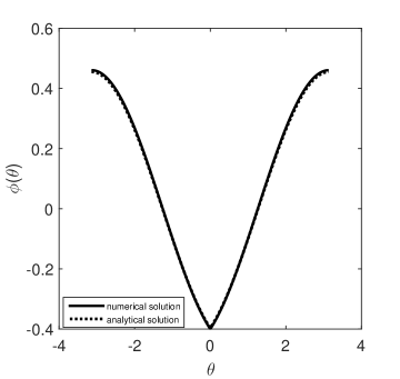
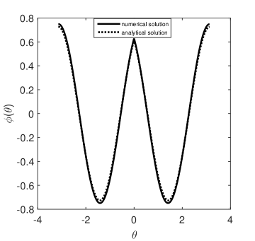
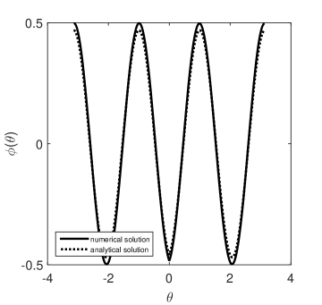
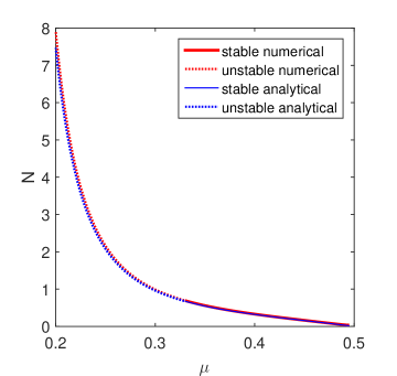
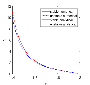
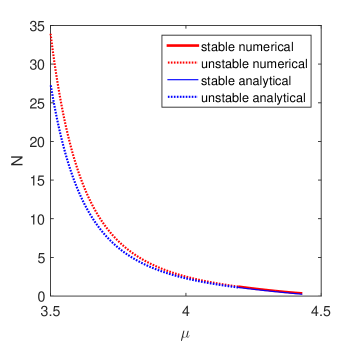
Figure 1: (a-c): Typical examples of stable analytical modes, given by Eqs. (12) and (13) for $\varepsilon=3$, and their counterparts, produced by the numerical solution of Eq. (8) using the regularized delta-function (26), with $\xi=0.01$. In panels (a), (b), and (c), the stationary solutions are displayed, severally, with the chemical potentials and norms $\left(\mu=0.35,N_{\mathrm{numerical}}=0.55,N_{\mathrm{analytical}}=0.54\right)$; $\left(\mu=1.66,N_{\mathrm{numerical}}=1.57,N_{\mathrm{analytical}}=1.53\right)$; and $\left(\mu=4.3,N_{\mathrm{numerical}}=0.69,N_{\mathrm{analytical}}=0.67\right)$, which places them in the first, second, and third bands, as defined by Eq. (16) with $n=0$, $1$, and $2$, respectively. (d-f): $N(\mu)$ curves for the analytical solutions, calculated as per Eqs. (14) and (13), and their numerically generated counterparts, in the first, second, and third bands, respectively. The full bands correspond to intervals $0.125<\mu<0.5$ ($n=0$), $1.125<\mu<2$ ($n=1$), and $3.125<\mu<4$ ($n=2$). Portions of the $N(\mu)$ curves, representing stable and unstable subfamilies of the stationary solutions, are designated as indicated in the notation boxes. Definitely unstable segments of the $N(\mu)$ curves, which correspond to extremely large values of $N$, are cut off by panel frames.

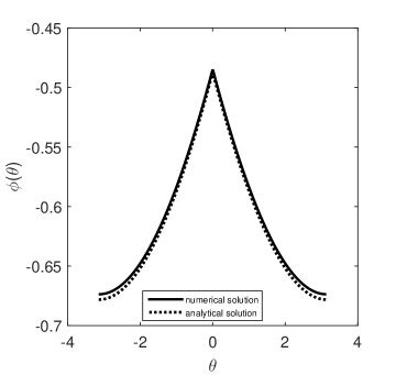
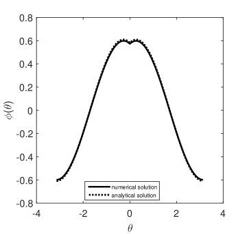
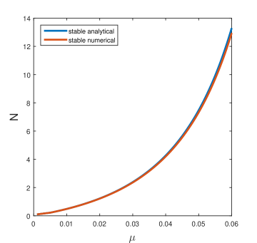
Figure 2: (a-c): Typical examples of analytical modes, given by Eqs. (12) and (13) with $\varepsilon=-1$, and their counterparts, produced by the numerical solution with $\xi=0.01$ in Eq. (26). In panels (a), (b), and (c) the chemical potential and norm take values $\left(\mu=0.03,N_{\mathrm{numerical}}=2.35,N_{\mathrm{analytical}}=2.38\right)$, $\left(\mu=0.6,N_{\mathrm{numerical}}=1.24,N_{\mathrm{analytical}}=1.26\right)$, and $\left(\mu=2.3,N_{\mathrm{numerical}}=4.20,N_{\mathrm{analytical}}=4.32\right)$, which places them in the first, second, and third bands, as defined by Eq. (17) with $n=0$, $1$, and $2$, respectively. The mode shown in (a) is a stable ground state, while ones in (b) and (c) are weakly unstable excited states. (d) The $N(\mu)$ curve for the analytical solution and its counterpart, produced by the numerical solution of Eq. (14) with $\xi=0.01$, in the first band, which covers the interval of $0<\mu<0.125$. This branch, representing the ground state, is completely stable. The branches of the excited states, populating the second and third bands, are not displayed, as they are subject to weak instability.

In terms of the local density, $\phi_{0}^{2}(x)$, the modes shown in Fig. 1 for $\varepsilon>0$ in the $n$-th band feature $2(1+n)$ peaks [i.e., $2$, $4$, and $6$ peaks in the first, second, and third bands, respectively, see Eq. (16)]. On the other hand, the modes displayed for $\varepsilon<0$ in Fig. 4, have, essentially, $2n$ peaks [i.e., $1$, $2$, and $4$ peaks in the first, second, and third bands, respectively, as per Eq. (17)], if the shallow splitting of the peak at $x=0$ is not counted for $n=1$ and $2$. In particular, the stationary mode in the first band, with the single density peak at $\theta=\pm\pi$, which is displayed in Fig. 2(a) (and is always stable, as shown below), may be identified as the ground state of the system with $\varepsilon<0$, as its energy, for given $N$, is always lowest, in comparison with the states found in the second and third bands. On the other hand, the multi-peak solutions, which populate the second, third (and higher-order) bands at $\varepsilon<0$, may be interpreted as excited states, always being weakly unstable, as shown below too. For $\varepsilon>0$, the identification of a ground state makes it necessary to consider solutions with $\mu<0$, which are addressed in the following subsection (recall that states with $\mu<0$ do not exist for $\varepsilon<0$).

It is worthy to note that all $N(\mu)$ curves displayed in Fig. 1 meet the above-mentioned VK criterion, $dN/d\mu<0$, thus having a chance to be (partly or entirely) stable. Further, in Fig. 2(d) the $N(\mu)$ dependence for $\varepsilon<0$ satisfies the anti-VK criterion HS , $dN/d\mu<0$, thus upholding the stability of the soliton family.

II.2 Solutions for $\mu<0$

In the infinite domain, negative values of the chemical potential correspond to pinned solitons (2), which, as said above, are completely unstable solutions. In the ring-shaped system, the relevant solution to Eq. (10), subject to b.c. (9), is

$$\phi(\theta)=\phi_{0}\cosh\left(\sqrt{-2\mu}\left(\pi-|\theta|\right)\right),$$ (18)

$$\phi_{0}^{2}=\frac{\sqrt{-2\mu}\sinh\left(\sqrt{-2\mu}\pi\right)}{\varepsilon\cosh^{3}\left(\sqrt{-2\mu}\pi\right)},$$ (19)

cf. Eqs. (12) and (13). As follows from Eq. (19), this solution exists, for $\mu<0$, solely in the case of the attractive nonlinearity, $\varepsilon>0$. The norm and energy of the solution for $\mu<0$, given by Eqs. (18) and 19), are

$$N=\phi_{0}^{2}\left[\pi+\frac{1}{2\sqrt{-2\mu}}\sinh\left(2\sqrt{-2\mu}\pi\right)\right],$$ (20)

$$H=\left(-\mu\right)\phi_{0}^{2}\left[\frac{1}{2\sqrt{-2\mu}}\sinh\left(2\sqrt{-2\mu}\pi\right)-\pi\right]-\frac{\varepsilon}{2}\phi_{0}^{4}\cosh^{4}\left(\sqrt{-2\mu}\pi\right).$$ (21)

It is relevant to note that the solution for $\mu<0$, given by Eqs. (18), (19) and (20), (21), can be obtained from the above one for $\mu>0$, based on Eqs. (12), (19), and (14), (15), as an analytical continuation from $\mu>0$ to $\mu<0$, according to the straightforward relations:

$$\sqrt{2\mu}=i\sqrt{-2\mu},~{}\sin\left(\sqrt{2\mu}\pi\right)=i\sinh\left(\sqrt{-2\mu}\pi\right),~{}\cos\left(\sqrt{2\mu}\pi\right)=\cosh\left(\sqrt{-2\mu}\pi\right).$$ (22)

A typical example of the mode with $\mu<0$, and the respective $N(\mu)$ and $H(N)$ dependences are displayed, along with their numerically found counterparts, in Fig. 3. Note that, unlike the solutions found above at $\mu>0$, whose norm may take indefinitely large values, diverging at the left edge of each band, as per Eqs. (14) and (13), straightforward analysis of Eqs. (20) and (19) reveals, as seen in Fig. 3(b), that at $\mu<0$ the norm is bounded from above by

$$N<N_{\max}\approx\allowbreak 1.\,\allowbreak 074/\varepsilon.$$ (23)

This largest value of the norm is attained at

$$\mu_{\max}\approx-0.150.$$ (24)

Further, the $H(N)$ dependence at $\mu<0$ features two branches in Fig. 3(c) in accordance with the fact that, in a narrow interval of norms, $N(\mu=-\infty)\equiv 1/\varepsilon<N<N_{\max}$ (i.e., $0.333<N<0.358$ for $\varepsilon=3$), two different values of $\mu$ correspond to given $N$. The solitons at $\mu<0$ always features a single density peak, like in Fig. 3(a).

The stability of these solutions is identified in the following section, by means of numerical methods. Actually, they are always subject to a (relatively weak) instability, even if the respective $N(\mu)$ dependence, as seen in Fig. 3(b), satisfies the VK criterion, $dN/d\mu<0$, in an interval of

$$0<-\mu<-\mu_{\max}\approx 0.150.$$ (25)

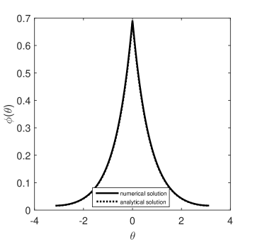
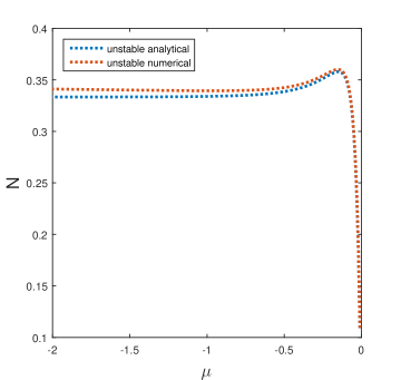
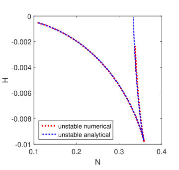
Figure 3: (a) A typical example of an [unstable, see Fig. 4(d) below] stationary mode existing at $\mu<0$, as produced by the analytical solution given by Eqs. (18) and (19), juxtaposed with the corresponding numerical solution of Eq. (8), for $\mu=-1$, $\varepsilon=3$ and $\xi=0.01$. The respective norms are $N_{\mathrm{numerical}}=0.342,N_{\mathrm{analytical}}=0.334$. (b,c) $N(\mu)$ and $H(N)$ curves for the analytical solutions, produced by Eqs. (20) and (21), and their numerically generated counterpart, for $\mu<0$ and $\varepsilon=3$. Unlike all other plots, the numerical ones in this panel were generated with $\xi=0.005$, to achieve sufficient accuracy.

Formally, the stationary solutions found at $\mu<0$ realize the ground state of the system with $\varepsilon>0$, as seen from the comparison of their negative energy, displayed in Fig. 3(c), with the positive energy of the solutions found, for the same values of $\varepsilon$ and $N$, at $\mu>0$. However, the instability of these stationary solutions suggests that the role of the ground state may be picked up by robust breathers which spontaneously develop from the unstable stationary states with $\mu<0$, see Fig. 5 below.

III Numerical solutions

III.1 Stationary solutions

In the numerical solution of the evolution and stationary equations (4) and (8), the delta-function was approximated by the standard regularized expression,

$${\tilde{\delta}}(\theta)=\frac{1}{\sqrt{\pi}\xi}\exp\left(-\frac{\theta^{2}}{\xi^{2}}\right),$$ (26)

with sufficiently small $\xi$. Stationary equation (8) with the regularized delta-function was numerically solved by means of the Newton-Raphson method, which is a root-finding algorithm that uses a truncated Taylor expansion to find a zero of a given function in a vicinity of an expected zero point Yang . Time-dependent solutions to Eq. (4) were then simulated by means of the split-step fast-Fourier-transform algorithm, which is well known to be appropriate for the NLSE Yang . The conservation of the integral norm and energy was monitored in all the dynamical simulations.

III.2 The linear-stability analysis: the Bogoliubov-de Gennes (BdG) equations

To analyze the stability of stationary solutions of Eq. (4) against small perturbations, perturbed solutions were taken in the usual form GPE ; Yang :

$$\psi\left(\theta,t\right)=e^{-i\mu t}\left\{\phi(\theta)+\eta\left[e^{-i\lambda t}u(\theta)+e^{i{\lambda}^{\ast}t}v^{\ast}(\theta)\right]\right\},$$ (27)

where $\eta$ is an infinitesimal amplitude of the perturbation, $u(\theta)$ and $v(\theta)$ represent its eigenmode, and $\lambda$ is the corresponding (generally, complex) perturbation eigenfrequency, the stability condition being $\mathrm{Im}\{\lambda\}=0$ for all $\lambda$ (the asterisk stands for the complex conjugate). The substitution of this expression in Eq. (4) and linearization (i.e., the derivation of the BdG equations for the small perturbations) leads, after straightforward manipulations, to the eigenvalue problem for $\lambda$, written in the matrix form:

$$\begin{pmatrix}\hat{L}&-\varepsilon\delta(\theta)\phi^{2}(\theta)\\ \varepsilon\delta(\theta)\phi^{2}(\theta)&-\hat{L}\end{pmatrix}\begin{pmatrix}u\\ v\end{pmatrix}=\lambda\begin{pmatrix}u\\ v\end{pmatrix},$$ (28)

where we define operator $\hat{L}\equiv-\mu-\frac{1}{2}d^{2}/d\theta^{2}-2\varepsilon\delta(\theta)|\phi|^{2}$, and the solution for $\left\{u(\theta),v(\theta)\right\}$ must satisfy the same b.c. (5) as above.

The numerical solution of Eq. (28), with the delta-function approximated as per Eq. (26), produces, for each stationary solution, a spectrum of eigenfrequencies $\lambda$. The analysis of the numerical data leads to conclusions about the stability of the modes with $\varepsilon>0$ (the self-attractive nonlinearity) and $\mu>0$, which are displayed in Table 1. It identifies stable and unstable subbands in each of the three lowest existence bands defined by Eq. (16).

$\mathrm{first~{}band~{}}(n=0)$	$\mathrm{second~{}band~{}}(n=1)$	$\mathrm{third~{}band~{}}(n=2)$
$0.125<\mu<0.5$	$1.125<\mu<2$	$3.125<\mu<4.5$
$\mathrm{stability~{}subband}$	$\mathrm{stability~{}subband}$	$\mathrm{stability~{}subbands}$
$0.337<\mu<0.5$	$1.66<\mu<1.70$	$4.194<\mu<4.5$

Table 1: Three lowest bands, corresponding to ${\small n=0}$, ${\small 1}$, and ${\small 2}$ in Eq. (16), in which the exact solutions, given by Eqs. (12) and (13), exists for ${\small\mu>0}$ and ${\small\varepsilon>0}$, and subbands in which they are stable, according to values of the perturbation eigenfrequencies produced by the numerical solution of the BdG equations for ${\small\varepsilon=3}$ and regularization parameter ${\small\xi=0.01}$ in Eq. (26).

In a detailed form, the same results which are summarized in Table 1, are displayed, in terms of the dependence of the largest instability growth rate of the perturbation, $\mathrm{Im}\{\lambda\}$, on $\mu$, along with respective $\mathrm{Re}\{\lambda\}$, in Figs. 4, where segments with $\mathrm{Im}\{\lambda\}=0$ represent stable stationary states. Actually, all complex eigenvalues exist in quartets, $\pm i\mathrm{Im}\{\lambda\}\pm\mathrm{Re}\{\lambda\}$, with independent signs $\pm$ in front of the imaginary and real parts. They reduce to double eigenvalues if either $\mathrm{Im}\{\lambda\}=0$ or $\mathrm{Re}\{\lambda\}=0$, the underlying solution being stable in the former case.

We stress that the existence of well-defined stable subbands in the second and third bands implies that the stationary modes with multi-peak shapes, see Figs. 1(b) and (c), may be stable in the present system, while most previously studied nonlinear systems with self-attractive nonlinearity admit only the stability of the simplest single-peak modes. On the other hand, the instability of all the states in each band with the norm exceeding a certain critical value, $N_{\mathrm{cr}}$, is explained by the fact the underlying equation (1) on the infinite line, with the ideal delta-function, gives rise to the critical collapse, because is maintains the TS family, as mentioned above (TS solutions exist precisely in the case when the critical collapse occurs Berge ; Fibich ; 1DTownes ). In particular, for the first band the numerical result, rescaled back to $\varepsilon=1$ [for comparison with Eq. (1)], yields

$$N_{\mathrm{cr}}\left(\varepsilon=1\right)=3N_{\mathrm{cr}}\left(\varepsilon=3\right)\approx 1.94,$$ (29)

i.e., almost exactly twice the above-mentioned critical value for Eq. (1), $N_{\mathrm{cr}}=1$. The doubling is explained by the shape of the mode displayed in Fig. 1(a): it is seen that approximately half of the total norm is placed around $\delta(\theta)$, and the other half is collected around the diametrically opposite position, $\theta=\pi$, the two peaks being separated by points where the local density vanishes.

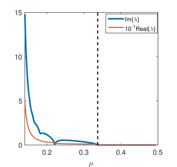
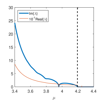
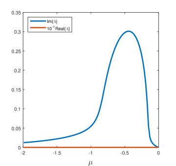
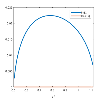
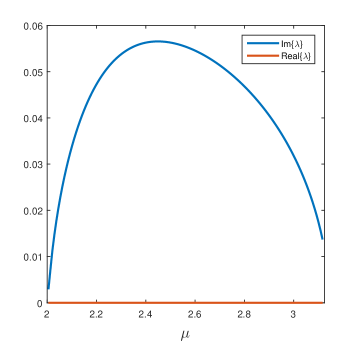
Figure 4: (a-d) Imaginary and real parts of the perturbation eigenfrequency, $\lambda$, vs. the chemical potential $\mu>0$, in the system with $\varepsilon=3$ and $\xi=0.01$. Panels (a), (b), and (c) display, respectively, the dependences for $\mu>0$ and $n=0$, $1$, and $2$ (c) in Eq. (16). Panel (d) displays the dependences for $\mu<0$. Only eigenfrequencies with the largest instability growth rate, $\mathrm{Im}\{\lambda\}$, are displayed, the underlying stationary modes being stable at $\mathrm{Im}\{\lambda\}=0$. Boundaries between stable and unstable subbands, which are specified in Table 1, are designated by vertical dashed lines. Panels (e) and (f) show the same, but in the case of the repulsive nonlinearity, $\varepsilon=-1$, in the second and third bands, which correspond to Eq. (17) with $n=1$ (a) and $n=2$ (b), respectively [the first band, corresponding to $n=0$, is not shown here, as it has $\mathrm{Im}(\lambda)\equiv 0$]. Note that $\mathrm{Im}\{\lambda\}$ is very small in (e) and (f).

According to the analytical result given by Eqs. (14) and (13), as well as according to what is seen in Figs. 1(d-f), the $N(\mu)$ dependences in all the three bands satisfy the VK criterion. However, this criterion does not apply to complex eigenvalues, being only relevant for purely imaginary ones, with $\mathrm{Re}\{\lambda\}=0$ Berge ; Fibich . This fact explains why only parts of the three bands carry stable modes, as shown by Table 1 and Figs. 4(a-c).

For the same $\varepsilon>0$, the stability of the single-peak stationary modes with $\mu<0$, such as the one shown in Fig. 3(a), is summarized in Fig. 4(d). It is seen that, strictly speaking, all such modes are unstable against perturbations with purely imaginary eigenfrequencies, in contradiction with the VK criterion, as Fig. 5 features $dN/d\mu<0$ in interval (25). However, the largest value of $\mathrm{Im}\{\lambda\}$ in this interval is actually very small in comparison with typical values of instability growth rates in other panels of Fig. 4. This fact suggests that the instability of the stationary solutions may be quite weak in this region, which is corroborated by direct simulations of the perturbed evolution, see Fig. 5(b) below. Actually, the instability of these single-peak modes, which are close to their counterparts supported by the delta-functional self-attractive cubic nonlinearity in the infinite domain [cf. solutions (18) and (2)], is a “remnant” of the instability of modes (2) in the infinite system.

Lastly, results of the linear-stability analysis for the stationary solutions with $\mu>0$, found in the model with the repulsive nonlinearity, $\varepsilon<0$, are summarized in Figs. 4(e,f). These solutions are completely stable in the first bandgap, which corresponds to $n=0$ in Eq. (17). This result is very natural, as the ground state in the model with the repulsive nonlinearity, which populates the lowest band, must be definitely stable. On the other hand, the excited states populating the second and third bands [which correspond, respectively, to $n=1$ and $2$ in Eq. (17], are weakly unstable, in formal contradiction with the anti-VK criterion. However, this weak instability does not really destroy the stationary modes from the second and third bands, see below.

III.3 Simulations of the perturbed evolution of stationary modes

The predictions for the stability and instability of the stationary modes, produced above by the solution of the BdG equations, have been verified by comparison with direct simulations of Eq. (4), in which the input was taken as the corresponding stationary modes with small random perturbations added to them. First, all the solutions which were predicted to be stable, viz., those belonging to the stable subbands in Table 1in the case of $\varepsilon>0$ and $\mu<0$, as well as ones belonging to the first band in the case of $\varepsilon<0$ and $\mu>0$, see Fig. 2(d), were found to be stable in the direct simulations, while the solutions belonging to unstable regions in Table 1 evolve into chaotic states (not shown here in detail).

Further, in the case of $\varepsilon<0$ and $\mu>0$, the perturbed evolution of two- and four-peak modes belonging to the second and third bands, where the numerical solution of the BdG equations yields very small values of the instability growth rate in Figs. (f,e), demonstrates small-amplitude oscillations around the persistent stationary modes (not shown here in detail). In other words, these modes remain effectively stable ones.

Lastly, direct simulations of the perturbed evolution of the stationary modes which are found, at $\varepsilon>0$, with $\mu<0$ demonstrate that their instability, predicted by the computation of perturbation eigenvalues in Fig. 4(d), leads to spontaneous transformation of the modes into robustly oscillating breathers, as shown in Fig. 5. The stationary solution which carries the largest instability growth rate, at $\mu=-0.5$ in Fig. 4(d), develops into a breather with large-amplitude oscillations [Fig. 5(a)]. On the other hand, Fig. 5(b) shows that, for $\mu$ close to point (24), at which the norm of the stationary model attains the maximum value (23), and the respective instability growth rate in Fig. 4(d) is quite small, the resulting breather features small-amplitude oscillations, hence it may be categorized as a nearly stable state.

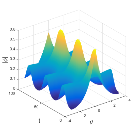
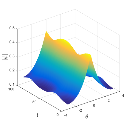
Figure 5: Direct simulations of the evolution of initially perturbed modes with $\mu<0$ for $\varepsilon=3$ and $\xi=0.01$, which are predicted to be unstable by the linear-stability analysis, see Fig. 4(d). Panels (a) and (b) pertain, respectively, to original stationary modes with $\mu=-0.5$, $N=0.344$ and $\mu=-0.17,N=0.36$, the latter one being close to the state with the largest norm, whose parameters are given by Eqs. (23) and (24).

IV Conclusion

The objective of this work is to generate basic stationary states in the model which is based on the one-dimensional Schrödinger equation on a ring, with the nonlinearity, of either attractive or repulsive sign, $\varepsilon>0$ or $\varepsilon<0$, concentrated at a single point, which may be represented by an ideal delta-function, or by a regularized narrow profile. In the case of the ideal delta-function, all the stationary solutions have been found in the exact analytical form. In particular, the stationary states with positive chemical potential, $\mu>0$, populate bands alternating for $\varepsilon>0$ / $\varepsilon<0$, and the stationary states with $\mu<0$ fill a semi-infinite band, solely for $\varepsilon>0$. While the exact solutions for $\mu<0$ are qualitatively similar to those previously reported for the ring with a pair of localized nonlinearities HPu , those for $\mu>0$, which were not found in previous works, provide a unique insight into exact bandgap states in the nonlinear model. The stability of the stationary states was investigated by means of numerical methods (the computation of perturbation eigenfrequencies and direct simulations of the perturbed evolution) in the three lowest bands for $\mu>0$, revealing that each band, in the case of $\varepsilon>0$, is split into stable and unstable subbands, the stability loss occurring with the increase of the total norm, $N$, at some critical level. Thus, multi-peak states, populating the higher (second and third) bands, are partly stable in them. In the case of the repulsive nonlinearity, the single-peak ground state is completely stable in the first band, while the two- and four-peak excited states in the two higher bands are weakly unstable in terms of their eigenvalues, staying virtually stable in direct simulations. In the case of the attractive self-interaction, the bound states with $\mu<0$ are subject to the instability which spontaneously transforms them into robust breathers. The latter instability is weak for the states with the norm close to the maxim value.

The analysis reported in this work can be extended for a more general setting, when a narrow stripe carrying a higher-order nonlinearity (e.g., quintic) is embedded into a medium with the uniformly distributed nonlinearity of a different type (e.g., cubic), as suggested by the analysis performed for the infinite domain in Ref. Radha . Another relevant direction may be the analysis of a model similar to the present one, but with two components, governed by nonlinearly coupled NLSEs, cf. Ref. Shnir .

References

- (1) F. Kh. Abdullaev and J. Garnier, Propagation of matter-wave solitons in periodic and random nonlinear potentials, Phys. Rev. A 72, 061605(R).
- (2) G. Theocharis, P. Schmelcher, P. G. Kevrekidis, and D. J. Frantzeskakis, Matter-wave solitons of collisionally inhomogeneous condensates, Phys. Rev. A 72, 033614 (2005).
- (3) Y. V. Kartashov, B. A. Malomed, and L. Torner, Solitons in nonlinear lattices, Rev. Mod. Phys. 83, 247-306 (2011).
- (4) L. P. Pitaevskii and A. Stringari, Bose-Einstein Condensation (Clarendon Press, Oxford, 2003).
- (5) B. A. Malomed and M. Ya. Azbel, Modulational instability of a wave scattered by a nonlinear center, Phys. Rev. B 47, 10402-10406 (1993).
- (6) Y. S. Kivshar and G. P. Agrawal, Optical Solitons: From Fibers to Photonic Crystals (Academic, San Diego, 2003).
- (7) J. Hukriede, D. Runde, and D. Kip, Fabrication and application of holographic Bragg gratings in lithium niobate channel waveguides, J. Phys. D 36, R1-R16 (2003).
- (8) K. Henderson, C. Ryu, C. MacCormick,and M. G. Boshier, Experimental demonstration of painting arbitrary and dynamic potentials for Bose-Einstein condensates, New J. Phys. 11, 043030 (2009).
- (9) D. M. Bauer, M. Lettner, C. Vo, G. Rempe and S. Dürr, Control of a magnetic Feshbach resonance with laser light, Nature Phys. 5, 339-342 (2009).
- (10) R. Yamazaki, S. Taie, S. Sugawa, and Y. Takahashi, Submicron spatial modulation of an interatomic interaction in a Bose-Einstein condensate, Phys. Rev. Lett. 105, 050405 (2010).
- (11) L. W. Clark, L.-C. Ha, C.-Y. Xu, and C. Chin, Quantum dynamics with spatiotemporal control of interactions in a stable Bose-Einstein condensate, Phys. Rev. Lett. 115, 153301 (2015).
- (12) R. Y. Chiao, E. Garmire, and C. H. Townes, Self-trapping of optical beams, Phys. Rev. Lett. 13, 479-482 (1964).
- (13) M. Vakhitov and A. Kolokolov, Stationary solutions of the wave equation in a medium with nonlinearity saturation, Radiophys. Quant. Electron. 16, 783-789 (1973).
- (14) L. Bergé, Wave collapse in physics: principles and applications to light and plasma waves, Phys. Rep. 303, 259-370 (1998).
- (15) G. Fibich, The Nonlinear Schrödinger Equation: Singular Solutions and Optical Collapse (Springer: Heidelberg, 2015).
- (16) N. Dror and B. A. Malomed, Solitons supported by localized nonlinearities in periodic media, Phys. Rev. A 83, 033828 (2011).
- (17) F. Kh. Abdullaev and M. Salerno, Gap-Townes solitons and localized excitations in low-dimensional Bose-Einstein condensates in optical lattices, Phys. Rev. A 72, 033617 (2005).
- (18) V. A. Brazhnyi and V. V. Konotop, Theory of nonlinear matter waves in optical lattices, Mod. Phys. Lett. B 18, 627-651 (2004).
- (19) O. Morsch and M. Oberthaler, Dynamics of Bose-Einstein condensates in optical lattices, Rev. Mod. Phys. 78, 179-215 (2006).
- (20) F. Lederer, G. I. Stegeman, D. N. Christodoulides, G. Assanto, M. Segev, and Y. Silberberg, Discrete solitons in optics, Phys. Rep. 463, 1-126 (2008).
- (21) H. Sakaguchi and B. A. Malomed, Solitons in combined linear and nonlinear lattice potentials, Phys. Rev. A 81, 013624 (2010).
- (22) H. Sakaguchi and B. A. Malomed, Matter-wave soliton interferometer based on a nonlinear splitter, New J. Phys. 18, 025020 (2016).
- (23) H. Sakaguchi, B. Li, E. Ya. Sherman, and B. A. Malomed, Composite solitons in two-dimensional spin-orbit coupled self-attractive Bose-Einstein condensates in free space, Romanian Rep. Phys. 70, 502 (2018).
- (24) T. Mayteevarunyoo, B. A. Malomed, and G. Dong, Spontaneous symmetry breaking in a nonlinear double-well structure,. Phys. Rev. A 78, 053601 (2008).
- (25) A. Acus, B. A. Malomed, and Y. Shnir, Spontaneous symmetry breaking of binary fields in a nonlinear double-well structure, Physica D 241, 987 - 1002 (2012).
- (26) R. Schützhold, M. Uhlmann, Y. Xu, and U. R. Fischer, Sweeping from the superfluid to the Mott phase in the Bose-Hubbard model, Phys. Rev. Lett. 97, 200601 (2006).
- (27) J. A. Sauer, M. D. Barrett, and M. S. Chapman, Storage ring for neutral atoms, Phys. Rev. Lett. 87, 270401 (2001).
- (28) S. Gupta, K. W. Murch, K. L. Moore, T. P. Purdy, and D. M. Stamper-Kurn, Bose-Einstein condensation in a circular waveguide, Phys. Rev. Lett. 95, 143201 (2005).
- (29) A. S. Arnold, C. S. Garvie, and E. Riis, Large magnetic storage ring for Bose-Einstein condensates, Phys. Rev. A 73, 041606(R) (2006).
- (30) O. Morizot, Y. Colombe, V. Lorent, H. Perrin, and B. M. Garraway, Ring trap for ultracold atoms, Phys. Rev. A 74, 023617 (2006).
- (31) A. Ramanathan, K. C. Wright, S. R. Muniz, M. Zelan, W. T. Hill, III, C. J. Lobb, K. Helmerson, W. D. Phillips, and G. K. Campbell, Superflow in a toroidal Bose-Einstein condensate: An atom circuit with a tunable weak link, Phys. Rev. Lett. 106, 130401 (2011).
- (32) B. E. Sherlock, M. Gildemeister, E. Owen, E. Nugent, and C. J. Foot, Time-averaged adiabatic ring potential for ultracold atoms, Phys. Rev. A 83, 043408 (2011); Erratum: Phys. Rev. A 83, 059904 (2011).
- (33) S. Moulder, S. Beattie, R. P. Smith, N. Tammuz, and Z. Hadzibabic, Quantized supercurrent decay in an annular Bose-Einstein condensate, Phys. Rev. A 86, 013629 (2012).
- (34) K. C. Wright, R. B. Blakestad, C. J. Lobb, W. D. Phillips, and G. K. Campbell, Driving phase slips in a superfluid atom circuit with a rotating weak link, Phys. Rev. Lett. 110, 025302 (2013).
- (35) S. Eckel, J. G. Lee, F. Jendrzejewski, N. Murray, C. W. Clark, C. J. Lobb,W. D. Phillips, M. Edwards, and G. K. Campbell, Hysteresis in a quantized superfluid “atomtronic” circuit, Nature 506, 200-203 (2014).
- (36) S. G. Johnson, M. Ibanescu, M. Skorobogatiy, O. Weisberg, T. D. Engeness, M. Soljačić, S. A. Jacobs, J. D. Joannopoulos, and Y. Fink, Low-loss asymptotically single-mode propagation in large-core OmniGuide fibers, Opt. Exp. 9, 748-779 (2001).
- (37) M. Ibanescu, S. G. Johnson, M. Soljačić, J. D. Joannopoulos, Y. Fink, O. Weisberg, T. D. Engeness, S. A. Jacobs, and M. Skorobogatiy, Analysis of mode structure in hollow dielectric waveguide fibers, Phys. Rev. E 67, 046608 (2003).
- (38) Z. Ruff, D. Shemuly, X. A. Peng, O. Shapira, Z. Wang, and Y. Fink, Polymer-composite fibers for transmitting high peak power pulses at 1.55 microns, Opt. Exp. 18, 15697-15703 (2010).
- (39) J. Scheuer and A. Yariv, Coupled-waves approach to the design and analysis of Bragg and photonic crystal annular resonators, IEEE J. Quant. Elect. 39, 1555-1562 (2003).
- (40) J. Scheuer and A. Yariv, Circular photonic-crystal resonators, Phys. Rev. E 70, 036603 (2004).
- (41) J. Scheuer, W. M. J. Green, G. A. DeRose, and A. Yariv, Lasing from a circular Bragg nanocavity with an ultrasmall modal volume, Appl. Phys. Lett. 86, 251101 (2005).
- (42) J. Scheuer and B. Malomed. Annular gap solitons in Kerr media with circular gratings. Phys. Rev. A 75, 063805 (2007).
- (43) Q. E. Hoq, P. G. Kevrekidis, D. J. Frantzeskakis, and B. A. Malomed, Ring-shaped solitons in a “dartboard” photonic lattice, Phys. Lett. A 341, 145-155 (2005).
- (44) X. Wang, Z. Chen, and P. G. Kevrekidis, Observation of discrete solitons and soliton rotation in optically induced periodic ring lattices, Phys. Rev. Lett. 96, 083904 (2006).
- (45) D. Burak and R. Binder, Cold-cavity vectorial eigenmodes of VCSEL’s, IEEE J. Quant. Elect. 33, 1205-1215 (1997).
- (46) A. Valle, Selection and modulation of high-order transverse modes in vertical-cavity surface-emitting lasers, IEEE J. Quant. Elect. 34, 1924-1932 (1998).
- (47) M. Miller, M. Grabherr, R. King, R. Jager, R. Michalzik, and K. J. Ebeling, Improved output performance of high-power VCSELs, IEEE J. Sel. Top. Quant. Elect. 7, 210-216 (2001)
- (48) X. F. Li, W. Pan, B. Luo, M. Da, and G. Peng, Theoretical analysis of multi-transverse-mode characteristics of vertical-cavity surface-emitting lasers, Semicond. Sci. Tech. 20, 505-513 (2005).
- (49) J.-Y. Yan, L. Li, and J. Xiao, Ring-like solitons in plasmonic fiber waveguides composed of metal-dielectric multilayers, Opt. Exp. 20, 1945-1952 (2012).
- (50) H. Deng Y. Chen, N. C. Panoiu, B. A. Malomed, and F. Ye, Surface modes in plasmonic Bragg fibers with negative average permittivity, Opt. Exp. 26, 2559-2568 (2018).
- (51) L. Lu, J. D. Joannopoulos, and M. Soljačić, Topological photonics, Nature Photonics 8, 821-829 (2014).
- (52) M. Leder, C. Grossert, L. Sitta, M. Genske, A. Rosch, and M. Weitz, Real-space imaging of a topologically protected edge state with ultracold atoms in an amplitude-chirped optical lattice, Nature Commun. 7, 13112 (2016).
- (53) Z. Yang, F. Gao, X. Shi, X. Lin, Z. Gao. Y. Chong, and B. Zhang, Topological acoustics, Phys. Rev. Lett. 114, 114301 (2015).
- (54) A. B. Khanikaev, S. H. Mousavi, W.-K. Tse, M. Kargarian, A, H. Mac-Donald, and G. Shvets, Photonic topological insulators, Nature Mater. 12, 233-239 (2012).
- (55) M. C. Rechtsman, J. M. Zeuner, Y. Plotnik, Y. Lumer, D. Podolsky, F. Deisow, S. Nolte, M. Segev, and A. Szameit, Photonic Floquet topological insulators, Nature 496, 196-200 (2013).
- (56) W.-J. Chen, S.-J. Jiang, X.-D. Chen, B. Zhu, L. Zhou, J.-W. Dong, and C. T. Chan, Experimental realization of photonic topological insulator in a uniaxial waveguide, Nature Commun. 5, 5782 (2014).
- (57) A. V. Nailov, D. D. Solnyshkov, and G. Malpuech, Polariton topological insulator, Phys. Rev. Lett. 114, 116401 (2015).
- (58) M. A. Bandres, M. C. Rechtsman, and M. Segev, Topological photonic quasicrystals: Fractal topological spectrum and protected transport, Phys. Rev. X 6, 011016 (2016).
- (59) Y. V. Kartashov and D. V. Skryabin, Modulational instability and solitary waves in polariton topological insulators, Optica 3, 1228-1236 (2016).
- (60) Y. V. Kartashov and D. V. Skryabin, Bistable topological insulator with excitons-polaritons, Phys. Rev. Lett. 119, 253904 (2017).
- (61) D. R. Gulevich, D. Yudin, D. V. Skryabin, I. V. Iorsh, and I. A. Shelykh, Exploring nonlinear topological states of matter with exciton-polaritons: Edge solitons in kagome lattice, Sci. Rep. 7, 1780 (2017).
- (62) C. Li, F. Ye, X. Chen, Y. V. Kartashov, A. Ferrando, L. Torner, and D. V. Skryabin, Lieb polariton topological insulators, Phys. Rev. B 97, 081103(R) (2018).
- (63) G. Harari, M. A. Bandres, Y. Lumer, M. C. Rechtsman, Y. D. Chong, M. Khajavikhan, D. N. Christodoulides, and M. Segev, Topological insulator laser: Theory, Science 359, 4003 (2018).
- (64) M. A. Bandres, S. Wittek, G. Harari, M. Parto, J. Ren, M. Segev, D. N. Christodoulides, and M. Khajavikhan, Topological insulator laser: Experiment, Science 359, eaar4005 (2018).
- (65) Y. V. Kartashov, V. A. Vysloukh, and L. Torner, Rotary solitons in Bessel optical lattices, Phys. Rev. Lett. 93, 093904 (2004).
- (66) Y. V. Kartashov, A. A. Egorov, V. A. Vysloukh, and L. Torner, Rotary dipole-mode solitons in Bessel optical lattices, J. Opt. B: Quant. Semicl. Opt. 6, 444-447 (2004).
- (67) B. Baizakov, B. A. Malomed, and M. Salerno, Matter-wave solitons in radially periodic potentials, Phys. Rev. E 74, 066615 (2006).
- (68) A. V. Yulin, Yu. V. Bludov, V. V. Konotop, V. Kuzmiak, and M. Salerno, Superfluidity of Bose-Einstein condensates in toroidal traps with nonlinear lattices, Phys. Rev. A 84, 063638 (2011).
- (69) X.-F. Zhou, S.-L. Zhang, Z.-W. Zhou, B. A. Malomed, and H. Pu, Bose-Einstein condensation on a ring-shaped trap with nonlinear double-well potential, Phys. Rev. A 85, 023603 (2012).
- (70) J. Yang, Nonlinear Waves in Integrable and Nonintegrable Systems (SIAM: Philadelphia, 2010).
- (71) H. Fabrelli, J. B. Sudharsan, R. Radha, A. Gammal, and B. A. Malomed, Solitons under spatially localized cubic-quintic-septimal nonlinearities, J. Optics 19, 075501 (2017).