Metals, depletion and dimming: decrypting dust

Abstract

Dust plays a pivotal role in the chemical enrichment of the interstellar medium. In the era of mid/high resolution spectra and multi-band spectral energy distributions, testing extinctions against gas and dust-phase properties is becoming possible. In order to test relations between metals, dust and depletions, and comparing those to the Local Group (LG) relations, we build a sample of 93 $\gamma$-ray bursts and quasar absorbers (the largest sample so far) which have extinction and elemental column density measurements available. We find that extinctions and total column density of the volatile elements (Zn, S) are correlated (with a best-fit of dust-to-metals (DTM) $4.05\times 10^{-22}$ mag cm²) and consistent with the LG DTM relation. The refractory elements (Fe, Si) follow a similar, but less significant, relation offset about 1 dex from the LG relation. On the assumption that depletion onto dust grains is the cause, we compute the total (gas$+$dust-phase) column density and find a remarkable agreement with the LG DTM relation: a best-fit of $4.91\times 10^{-22}$ mag cm². We then use our results to compute the amount of ‘intervening metal from unknown sources’ in random sightlines out to redshifts of $z=5$. Those metals implicate the presence of dust and give rise to an average ‘cosmic dust dimming’ effect which we express as a function of redshift, CDD($z$). The CDD is unimportant out to redshifts of about 3, but because it is cumulative it becomes significant at redshifts $z=3-5$. Our results in this paper are based on a minimum of assumptions and effectively relying on observations.

1 Introduction

Interstellar dust plays a crucial role in the chemical enrichment of the interstellar medium (ISM) and is strongly linked with star formation (e.g. Cortese et al., 2012). Extinction, $A_{V}$, is the scattering and absorption of photons along the travel path from a source to the observer. Depletions of heavy elements in the ISM are another way to study dust properties due to its association with dust (Jenkins, 1987). Depletion is a strong indicator that gas phase refractory element ejected from stars is efficiently condensed onto ISM dust grains. The dust grains are primarily made up of O, Si, C, Mg, and Fe metals (Draine, 2003; De Cia et al., 2016) which are introduced into the ISM through the stellar winds during the stellar evolution or at the end of the life of a star. However, there is still a debate over the origin of the bulk of dust, where various candidates have been proposed such as: $i)$ dense envelopes of evolved, low-mass asymptotic giant branch (AGB) stars (Gail et al., 2009), $ii)$ condensation in supernova ejecta (Dunne et al., 2003), and $iii)$ grain growth in the dense molecular clouds (Draine, 2009).

The dust-to-metal ratios over cosmic time provide information on the interplay between dust and gas in the ISM of galaxies. Theoretical studies show dust-to-metals ratios to remain constant over time and metallicity, provided both dust and metals are produced in and ejected from stars (e.g., Franco & Cox, 1986). In a sample of gamma-ray burst (GRB) afterglows, foreground quasar absorbers, and lensed galaxies (Chen et al., 2013), Zafar & Watson (2013) found that the dust-to-metals ratios remain constant over a wide range of redshifts, metallicities, hydrogen column densities, and galaxy types. The dust-to-metals ratios in their sample are consistent with the Local Group (LG) relation. A dust model for cosmological simulations shows that for a constant dust-to-metals ratios most of the dust is produced in supernovae (Mattsson et al., 2014; McKinnon et al., 2016). There is a discrepancy between using direct line-of-sight extinctions and depletion derived dust measures. The depletion derived dust content suggests dust-to-metals are correlated with metallicity (De Cia et al., 2016; Wiseman et al., 2017; De Vis et al., 2017). Using depletion derived dust methods, individual objects (Watson et al., 2006; Savaglio et al., 2012; Friis et al., 2015) and samples (Wiseman et al., 2017) find mis-match with the observed $A_{V}$. For such a scenario models (Mattsson et al., 2014; Schneider et al., 2016; Zhukovska et al., 2016; Popping et al., 2017) suggest grain growth in the ISM is dominant dust production pathway.

Extinction is caused by the dust particles in the ISM, therefore, $A_{V}$ should scale with the column density of atoms in the dust-phase. The Milky Way (MW) refractory elements dust-phase column density and $A_{V}$ follow each other (Vladilo et al., 2006). A small sample of damped Ly$\alpha$ absorbers (DLAs) along the line of sights of quasars (QSOs) are reported to follow the MW relation (Vladilo et al., 2006). A similar correlation is also seen for a small sample of GRBs where exclusion of the cases with a 2175 Å bump feature strengthen the correlation (De Cia et al. 2013; see however Wiseman et al. 2017 but with a large scatter).

Dust-to-metal ratios for DLAs have also been derived from depletions using depletion corrections from the Galactic or disk$+$halo environments (Savaglio, 2001; De Cia et al., 2013). In this paper, we test the connections between extinction and depletions in a significantly larger sample combined of both GRBs and QSO-DLAs, but here adopting methods with a minimum of assumptions and using mostly direct observables. The aim of our investigation is both to test the above-mentioned relations and test for connections between the two quantities and other observables which lead us to infer effect of dust at cosmological distances. For this, we need high redshift measurements of extinctions, elemental abundances of refractory and volatile elements, and hydrogen column densities of the systems if possible. In §2 we present our sample and sample selection criteria. In §3 we describe our methods used for the investigation together with the results of the analysis. The discussion is provided in §4 and conclusions are given in §5. Throughout the paper, errors are 1$\sigma$ unless stated otherwise.

2 Sample Selection

We searched the literature carefully and selected all published GRB-DLAs and QSO-DLAs sightlines conforming to our requirements which are as follows. The object must have spectral energy distributions (SEDs) and optical spectroscopic data available with measurements of $A_{V}$, column densities of Zn ii and Fe ii, or of S ii and Si ii. The GRBs are selected only if they had their optical extinction derived from simultaneous SED fitting to X-ray$-$to$-$optical/NIR data using either a single or broken power-law (see Zafar et al. 2011; Greiner et al. 2011; Schady et al. 2012; Covino et al. 2013; Bolmer et al. 2018 for discussion on $A_{V}$ determination). This is a reliable method to determine extinctions at higher redshifts where the intrinsic slopes are constrained by the X-ray data. Note that there is some degeneracy between broken power-law break frequency and extinction, which could lead to inference of grey dust for some instances (Watson et al., 2006; Perley et al., 2008; Friis et al., 2015). However, overall a fixed spectral break change ($\Delta\beta=0.5$) between the optical and X-ray slopes is preferred for GRBs (Greiner et al., 2011; Zafar et al., 2011; Japelj et al., 2015). For QSO-DLAs, reddening must be determined either from QSO colors or extinctions through template fitting to the QSO SED. Those methods are less robust than the X-ray supported GRB fits, but are widely adapted. We refer the reader to Zafar et al. (2015); Krogager et al. (2015, 2016) for more discussions on $A_{V}$ determination for QSO. The requirement for the pairs of elements (Zn ii and Fe ii, or of S ii and Si ii) are in order to be able to derive depletions. Here Zn and S are volatile elements and Fe and Si are refractory elements (e.g., Ledoux et al., 2002; Draine, 2003; Vladilo et al., 2011; De Cia et al., 2016). Defined this way our initial sample consists of 28 GRBs and 32 QSO-DLAs with the required measurements available. To this we add sources where only part of the required measurements are complete but where limits have been determined for the rest. The vast majority of the elemental abundances have been determined via detailed spectral line fitting, for eight GRBs elemental abundances (or limits) were derived from rest-frame equivalent widths of non-saturated lines provided by Fynbo et al. (2009) as described in Laskar et al. (2011) and Zafar & Watson (2013) (see references to Table 2).

In total this makes up a sample of 46 GRBs (see Table 2) and 47 QSO-DLAs (see Table 3), i.e. a total of 93 independent sightlines. The sample is a complete literature sample and as such inherits whichever biases went into the initial target selection for observation and publication, but no additional biases were introduced by us other than the selection definitions we provide above. The sample covers redshifts from the nearby Universe ($z\approx 0.4$) out to the epoch of reionisation ($z\approx$6.3) and is significantly larger than any other sample used for previous similar studies. Following the discussion of Watson (2011), we use solar abundances from Anders & Grevesse (1989) for metallicity and depletion determinations. Anders & Grevesse (1989) abundances are better estimates of the typical Galactic ISM (see also Asplund et al., 2009).

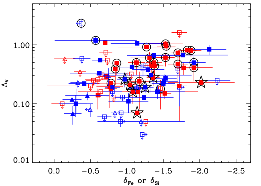
Figure 1: Extinctions against the iron or silicon depletions. The red color corresponds to QSO-DLA cases, while blue indicates GRB-DLA cases. For both, squares represent depletions determined from the [Fe/Zn] depletions and triangles show the [Si/S] depletions. Filled symbols are measurements while open symbols are limits. The black encircled data points highlight cases with a 2175 Å bump and starred are the cases with N(H₂) measurements.

3 Methods and results

The objective of this study is to test which relations are seen in the complete literature sample we have compiled, partly to clarify some concepts related to dust, metals, and depletion, but in particular to help future studies related to, or depending on, dust-to-metal ratios. We here use the term ‘dust-to-metal’ (or in short DTM) in the same way as it was introduced in Watson (2011). It is thought that depletion of metals, i.e. the metals ‘missing’ in sightlines based on a comparison to some expectation, is related to dust production, and therefore at some level should correlate with dust absorption. On the other hand, it is not the depletion alone which defines the amount of dust, obviously the amount of dust will grow with both the fraction of ‘missing’ metals, but also with the column density of the absorber. A first test should therefore be to ask which of the two is a most important quantity.

We therefore first compare the extinctions directly to depletions $\delta_{\rm(Fe)}$ and $\delta_{\rm(Si)}$ (Fig. 1). The depletions are calculated by comparing elements having a similar nucleosynthetic history. The iron peak element Fe is compared with iron peak element Zn and likewise $\alpha$-element compared with the other one from the chain (Si, S) such that $\delta_{\rm Fe}=$ log (N(Fe ii)/N(Zn ii)) $-$ log (Fe/Zn)_⊙ and similar for silicon. In Fig. 1 we plot $\delta_{\rm(Fe)}$ for each target if available (squares), and plot only $\delta_{\rm(Si)}$ (triangles) if $\delta_{\rm(Fe)}$ is not known. As can be seen from the figure there is no obvious strong correlation in this sample between reddening and depletion. This visual impression is confirmed by a statistical analysis which gives a correlation coefficient of $r=-0.16$ ($r=-0.05$ ignoring the data providing only limits) with a significance of only $\approx 87\%$. The weak correlation is not very surprising because of the wide range of H i column densities of the sample.

[Fe/Zn] is found to be a reliable tracer of dust in the ISM (De Cia et al., 2016; De Cia, 2018). However, for high-redshift sources this measurement is missing because of the available spectral coverage. We, therefore, chose [Si/S] as tracer of dust in high-redshift sources. We also attempted to correct [Si/S] using De Cia et al. (2016) correlations but as we later cannot make better use of it (see §3.2), therefore, we kept using [Si/S] for the cases where [Fe/Zn] is not available.

3.0.1 Zn and S depletion

We considered Zn and S as volatile elements to derive equivalent metal column densities. For QSO-DLAs, Zn (De Cia et al., 2016) and for Galactic sightlines, S (Jenkins, 2009; Jenkins & Wallerstein, 2017) are reported to be depleted. However, for a sample of 293 QSO-DLAs, Vladilo et al. (2011) discussed about using S and Zn as volatile elements. We refer to the reader to their section 2.5 for more discussion on selection of these elements. Briefly outlining, S and Zn are depleted in highly depleted Galactic sightlines (Jenkins, 2009; Jenkins & Wallerstein, 2017). Scappini et al. (2003) have discussed chemical pathways leading to S depletion in molecular clouds. DLAs are typically less dusty (compared to Galactic sightlines) and have less molecular detection, so Zn and S will be mostly undepleted. Noterdaeme et al. (2008b) and Savage & Sembach (1996) find that molecular fraction is correlated with depletions for DLAs and Galactic ISM, respectively. Considering this, we expect Zn or S depletion for the cases where we have high molecular fraction. However, searching in the literature we find only seven (out of 93) cases have molecules detection. Moreover, S is a troublesome element (Jenkins & Wallerstein, 2017) for Galactic sightlines and for DLAs because of blending with the Ly$\alpha$ forest. Super-solar Galactic S abundances (Jenkins, 2009) are found for low column density (N(H i)$<10^{19.5}$ cm^-2) sightlines. In case of DLAs, gas is predominantly neutral above N(H i)$>10^{19.5}$ cm^-2 (e.g., Meiring et al. 2009, see also Wolfe et al. 2005). In our sample, we mostly have systems with N(H i)$>10^{19.5}$ cm^-2 except one, therefore, we should not see such a behaviour.

3.1 Correlation with metal column densities

Total column densities of a given element are direct observables, and we now wish to test if those correlate with $A_{V}$ in our sample. In order to make the data simple to compare to the Local Group $N_{H}-A_{V}$, and also to be able to inter-compare different elements, we follow the strategy used by Zafar & Watson (2013) and first apply a simple modification to the data. We refer the reader to Zafar & Watson (2013) for more details on the method. For a given object, and a given volatile element ‘X’, we first determine the metallicity from that element [X/H] and then we multiply logarithmic metallicity with N(H i) such that it becomes N(H i)$\times 10^{\rm[X/H]}$. This has the advantage of shifting each element to the $N_{H_{X}}$ (equivalent soft X-ray H i column density) used by Watson (2011) to determine the $A_{V}$ of the Milky Way (MW).

Zafar & Watson (2013) found that the total metal column and extinction in their sample (26 measurements and 21 limits) follows the LG relation ($N_{H,X}=2.2\times 10^{21}$cm${}^{-2}A_{V}$ with $N_{H,X}/N$(H i)$=1.1$) derived by Watson (2011) from the photoelectric absorption of the soft X-ray of GRBs using the Galactic dust (Schlegel et al., 1998) and H i column density (Kalberla et al., 2005). The Zafar & Watson (2013) sample followed an average value of metals-to-dust ratio of $10^{21.2}$cm${}^{-2}A_{V}$mag^-1 and a standard deviation of 0.3 dex. In Fig. 2, upper panel, we plot the relation for our enlarged sample together with the LG soft X-ray relation (green dashed line, Watson, 2011). Throughout the paper, we used Pearson correlation to define a relation together with its coefficient and significance. We used linear regression to derive a best-fit slope and intercept. This is performed in IDL using its routine FIT_AND_CORRELATE. In case of fitting data with limits, we used IDL routine FITEXY incorporating upper and lower limits (see Kelly, 2007). In Fig. 2, a linear regression relation fit to the data gives a best-fit of $(4.05\pm 1.03)\times 10^{-22}$, similar to the LG relation. The significance of the correlation is reported in Table 1. Table 1 shows that correlation strengths with measurements only data are quite strong but drop when including limits because of adding more scatter. We also look into S depletion issue and re-fit the data by dropping S-based measurements. The correlation coefficient drops a little to $\rho=+0.47$ but the best-fit value is consistent within 1$\sigma$. This suggests that depletion effect is small for S in our sample.

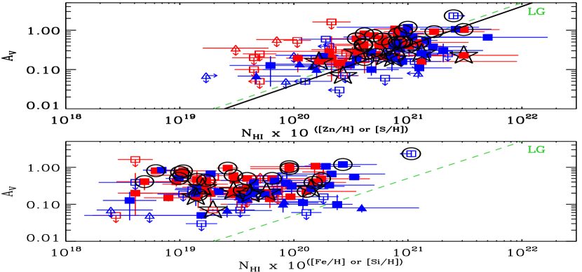
Figure 2: Extinctions against total equivalent column densities. The green dashed line represents the dust-to-metals ratio for the LG environments with the green dotted lines marking the its 1$\sigma$ range (Watson, 2011). In upper panel the black solid line shows the linear regression relation given in Table 1. The symbols and colors have the same meaning as in Fig. 1.

For the two refractory elements the observed equivalent metal column densities are plotted in the lower panel of Fig. 2. Here Si (triangles) is only plotted if Fe is not available. A linear regression fit although provides a similar slope with that of the volatile elements (Table 1) but has a very low significance. It is notable that for any given $A_{V}$ the values are shifted about 1 dex towards lower metallicity than the LG, thus confirming the depletion of those two elements. The fact that the slope of the relation is not changed is consistent with the conclusion (Fig. 1 above) that the depletions do not correlate with $A_{V}$. The shift of about 1 dex is also consistent with the average $\delta_{\rm(Fe,~{}Si)}$ of $\approx-1$.

3.2 Correlation with metal depletion

In Fig. 2 we could also directly see the effect of the depletion of refractory elements via grain formation. Where the volatile elements basically followed the curve for the LG, the refractory elements fell on average about one dex to the left of that, indicating that the residual amount of those elements was on average in our sample only about 10% .

Perhaps the best way to test the direct relation between $A_{V}$ and metal column density is to consider the elements which are depleted onto dust, such as Fe, but to add together the residual fraction left in the gas phase and that which has been depleted onto grains. Vladilo et al. (2006) showed that it is possible to compute e.g. the Fe dust-phase column density (N(Fe)_dust) for individual systems using

$${\rm N(Fe)}_{\rm dust}=(1-10^{\delta_{\rm Fe}}){\rm N(Zn})\bigg{(}\frac{{\rm Fe}}{{\rm Zn}}\bigg{)}_{\odot}$$ (1)

which is based on the assumption that intrinsically all absorbers have a Zn to Fe ratio identical to the solar. A similar equation can be written for S and Si

$${\rm N(Si)}_{\rm dust}=(1-10^{\delta_{\rm Si}}){\rm N(S})\bigg{(}\frac{{\rm Si}}{{\rm S}}\bigg{)}_{\odot}$$ (2)

based on a similar assumption about the intrinsic S to Si ratio. In Fig. 3 we plot $A_{V}$ vs ${\rm N(Fe)}_{\rm dust}$. Again, as above, in cases where ${\rm N(Fe)}_{\rm dust}$ is not available, but where we have ${\rm N(Si)}_{\rm dust}$, we plot the latter. In this plot we use the actual dust grain column density of the element, i.e. we are not converting as we did in Fig. 2. This means that we expect a small horizontal offset between the Fe and Si relation in Fig. 3, an offset which is much smaller than the scatter and for the purpose of a visual comparison we can ignore it. In the figure we again compare to the DTM relation of the MW (dashed green line), but here to the relation determined by Vladilo et al. (2006) using the same method as defined in equation 1. The agreement with our local environment in the MW is seen to be very good, the fit parameters are again provided in Table 1.

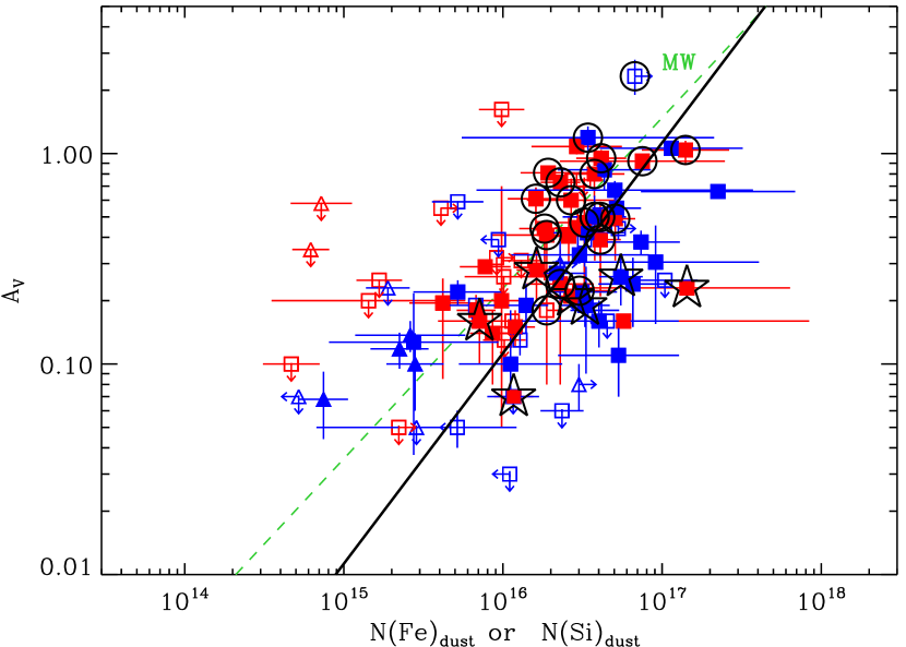
Figure 3: Extinctions as a function of dust-phase column densities. The green dashed line corresponds to the MW relation given in (Vladilo et al., 2006). The black solid line represents the linear regression relation with the best-fit value of $A_{V}/{\rm N(Fe)}_{\rm dust}=(1.13\pm 0.84)\times 10^{-17}$. The symbols and colors have the same meaning as in Fig. 1.

With this we are now able to compute the total column density also for the refractory elements. As noted, the offset in lower panel of Fig. 2 is due to dust depletion and if we correct for dust column, we would expect to see the similar behaviour of the lower panel as upper panel. We add ${\rm N(Fe)}_{\rm dust}$ and ${\rm N(Si)}_{\rm dust}$ to the observed gas phase column densities in order to obtain the total column densities of refractory elements (since ${\rm N(X)}_{\rm tot}={\rm N(X)}_{\rm dust}+{\rm N(X)}_{\rm obs}$). We can then derive the equivalent metal column densities of refractory elements (Fig. 4) in the same way as we did the gas phase columns in Fig. 2 i.e. first converting to equivalent H i column density.

The best-fit values of our and LG sample are in agreement. In fact the agreement is so complementary that we had to increase the linewidth of the LG curve and show our fit as a dashed line, because the fits were covering each other. We also plotted the error on the fit as gay shaded region (see Fig. 4), however, not that the scatter is not that small. Note that the correlation coefficient strength is not increased significantly when using the total equivalent column densities for refractory elements because of the internal scatter and inclusion of limits in the fit but the significance indicates the reliability of the fit. The agreement of LG relation and depletion-correction derived dust-to-metals best-fit values suggests that the time lag between dust formation after metal formation is small and they both grow together across different environments at all redshifts (see Zafar & Watson 2013 §3 for more discussions).

4 Discussion

We have assembled the by far largest sample of sightlines (93) for which both $A_{V}$ measurements and accurate low ionisation metal column densities are known. In this sample we have only included sightlines which contain measurements of at least one of the pairs (Zn, Fe), (S, Si) thereby allowing us always to correct at least one of the elements (Fe, Si) for assumed depletion. Starting from the lowest level of assumptions, i.e. simply testing if individual observed metal column densities scale with $A_{V}$, and moving to assuming that deviations from relative solar abundances can be interpreted as depletion, i.e. as metals removed from the gas-phase by dust grain growth, we have tested for correlations in the sample.

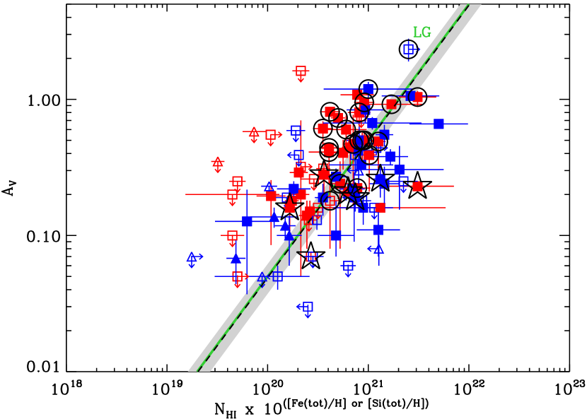
Figure 4: Total column density for the refractory (Fe or Si) elements. The green solid line is the LG relation given in Watson (2011). The black dashed line is the linear regression relation where grey shaded region represents error on it. The symbols and colors have the same meaning as in Fig. 1.

All the expected correlations are present in our sample. While this does not yet constitute a final confirmation, we conclude that our sample does indeed contain relations which are in full agreement with the conjectures that ($i$) the amount of dust scales directly with the amount of metals available and ($ii$) the dust column density also scales with the amount of dust. Note that there are also nucleosynthetic effects present which could be as large as 0.3 dex for DLAs (Rafelski et al., 2012; De Cia et al., 2016; Jenkins & Wallerstein, 2017; De Cia, 2018). As such this sample should prove a valuable tool to test and refine the current paradigms for dust creation and destruction. In particular its wide redshift coverage ($z=0.4-6.3$) provides support for studies aiming at identifying dust production mechanisms throughout the history of the universe.

4.1 Intervening non-related reddening

Along all lines of sight out to high redshift targets, a random number of intervening unidentified absorbers will be present. The combined effect of those absorbers (in case they contain dust) will be an additional reddening signature, but because the wavelength scales of dust absorption signatures are very large, individual random absorbers cannot be identified. Here we show that we can use our conclusions from the current work to compute the average statistical signature.

We have shown here that there is a strong dependence of $A_{V}$ on low ionisation metal column densities. Low ion metals can only exist if they are shielded from ionising radiation by H i. The amount of H i along a random sightline as a function of redshift has been extensively studied (e.g., Zwaan et al., 2005; Lah et al., 2007; Noterdaeme et al., 2012; Zafar et al., 2013). Here we shall use the recent results from Zafar et al. (2013) which provides the average number of DLAs per sightline in bins of $\Delta z\sim 0.5$ out to $z=5$. From their Table 6 we compute the average H i column density of DLAs in their sample at each redshift they studied, and find that it is effectively constant with redshift, log N(H i) = 20.85. DLAs are known to make up $\approx 85$% of all H i (Zafar et al., 2013). We correct for the remaining 15% (subtracting log(0.85) from the average) obtaining 20.92 which we then multiply on to each redshift bin to obtain the average N(H i) in each bin (shown as black points in Fig. 5).

Table 1: Pearson linear correlation coefficient, $\rho$ and significance, $\alpha$, together with the best-fit slope as $y/x$.

$x$	$y$	$y/x$	$\rho$	$\alpha$
Measurements only
$\delta_{\rm(Fe,Si)}$	$A_{V}$	$\cdots$	$-0.05$	$>$$28\%$
N(H i) $\times 10^{{\rm[Zn,S/H]}}$	$A_{V}$	$(3.98\pm 1.11)\times 10^{-22}$	$+$0.59	$>$$99\%$
N(H i) $\times 10^{{\rm[Fe,Si/H]}}$	$A_{V}$	$\cdots$	$+$0.06	$>$$36\%$
N(Fe, Si)dust	$A_{V}$	$(1.12\pm 0.78)\times 10^{-17}$	$+$0.62	$>$$99\%$
N(H i)$\times 10^{{\rm[Fe_{\rm tot},Si_{\rm tot}/H]}}$	$A_{V}$	$(6.92\pm 1.05)\times 10^{-22}$	$+$0.60	$>$$99\%$
Measurements and limits included
$\delta_{\rm(Fe,Si)}$	$A_{V}$	$\cdots$	$-0.16$	$\approx$$87\%$
N(H i) $\times 10^{{\rm[Zn,S/H]}}$	$A_{V}$	$(4.05\pm 1.03)\times 10^{-22}$	$+$0.49	$>$$99\%$
N(H i) $\times 10^{{\rm[Fe,Si/H]}}$	$A_{V}$	$\cdots$	$+$0.21	$\approx$$95\%$
N(Fe, Si)dust	$A_{V}$	$(1.13\pm 0.84)\times 10^{-17}$	$+$0.47	$>$$99\%$
N(H i)$\times 10^{{\rm[Fe_{\rm tot},Si_{\rm tot}/H]}}$	$A_{V}$	$(4.91\pm 0.98)\times 10^{-22}$	$+$0.51	$>$$99\%$

The average metallicity evolution of the H i gas has been vividly debated in the past, but the consensus is now that there is (as one would also logically expect) a general increase in metallicity as a function of cosmic time. Here we use the ‘best fit line’ from figure 12 in Rafelski et al. (2012). It has a slope of $-0.193$ dex per unit redshift, and for illustration purposes we plot it in red in Fig. 5 at a convenient offset. Using the average metallicity of each redshift bin we now compute how much Fe (total, including both gas-phase and dust-phase) there is in each bin. This is plotted as the blue points. It is seen that the higher line-of-sight H i column density per unit redshift in the past is perfectly balanced by the redshift evolution of metallicity, leaving the amount of metals per unit redshift remarkably constant (note that the first two and the last bin are slightly larger than 0.5). At high redshifts, the change in relative contributions of dust producers (Bolmer et al., 2018; Zafar et al., 2018a) could also change the effect of total Fe on extinction.

It is now simple to compute the average total column density of Fe along a sightline back to a given redshift, and then use the fit in Fig. 4 to convert this to an average ‘cosmic dust dimming’ CDD($z$). In Fig. 6, we provide this quantity, CDD($z$), back to a redshift of $z=5$.

4.2 Impact on high redshift surveys

Fig. 6 shows the accumulated effect of dust in random sightlines out to cosmological distances. It is seen that up to redshifts of about 3 the CDD($z$) is smaller than the typical uncertainties on individual $A_{V}$ measurements, and the effect can be ignored without too much impact. At redshifts in excess of 4, in the current paradigm, the CDD($z$) continues to rise despite the dropping metallicity, causing the cumulated effect to become significant. It should be recalled that the curve shows the average, but the effect is highly stochastic. Therefore corrections and predictions should probably only be considered for statistical samples while the effect on individual objects will be stochastic.

4.3 Inclusion of 2175 Å bump

The shape of the extinction curve tells us about the dust grains in the ISM (Draine, 2003). Carbonaceous dust grains are responsible for the 2175 Å bump and silicates induce the steepness in the extinction curve (Weingartner & Draine, 2001; Draine, 2003). We here aim to see if different extinction curves carrying different dust grain properties could effect our results. Our sample mostly has preference towards featureless Small Magellanic Cloud (SMC)-type extinction curve. However, 21 cases (3 GRBs and 18 QSO-DLAs) are reported to contain a 2175 Å bump, suggesting carbonaceous dust enriched environments. These cases are highlighted by stars drawn around the data points in Fig. 1–4.

De Cia et al. (2013) presented a sample of 18 GRBs (11 measurements and 7 limits) which included a single burst with a 2175 Å extinction feature (GRB 070802). That single burst did not fall on the $A_{V}$ and N(Fe)_dust relation of their limited sample, and De Cia et al. (2013) suggested that objects with the 2175 Å bump might follow a different relation and therefore should not be included. Our larger sample includes 19 sightlines with bumps, and is reaching extinctions 1.8 mag higher than the De Cia et al. (2013) sample, but we see no evidence that the 2175 Å bump cases follow a different relation. We also find that inclusion of the 2175 Å bump cases strengthens the relation especially at higher extinctions. Depending on the amount of metals available to form dust, different grain compositions and sizes could provide a range of optical extinction laws.

Figure 5: Total N(H i) per redshift bin against redshift is shown as black symbols. Total N(H i) for each redshift bin is computed using absorber number density, $d(n)/dz$, from Zafar et al. (2013). The average metallicity evolution (offset for illustration) from Rafelski et al. (2012) is shown as red curve. Blue points indicate total Fe (including both gas and dust-phase) calculated using total N(H i) and metallicity.

4.4 Dust-to-gas ratios and molecules

We would expect a general trend that on average an absorber with a large N(H i) should have a large $A_{V}$. The general trend will be modified both by the intrinsic scatter visible in figures 2-4, but also by the significant width of the metallicity distribution. In addition to this there are systematic selection differences between GRBs and QSOs, e.g. that GRBs are found closer to the centres of galaxies and at higher redshifts than QSO sightlines, causing their N(H i) to be systematically large and metallicities to be systematically low. Such effects will distort the N(H i) versus $A_{V}$ and the N(H i) versus N(Fe, Si)_dust relations.

Molecular gas is expected to have an even stronger correlation with dust than the neutral gas. Dust plays a major role for the presence of molecular gas by catalysing the formation of molecules on the surface of dust grains as well as shielding against Lyman-Werner photons. However, our sample contains only seven sightlines with available N(H₂) measurements, and no obvious relation is seen in the present sample. A larger sample of sightlines with molecule detections is required for this and should be a primary goal for future samples.

Figure 6: The average ‘cosmic dust dimming’, CDD($z$), is computed as the integrated $A_{V}$ from redshift 0 to $z$. The $A_{V}$ is computed from the average amount of dust along the line of sight based on the distribution of Fe (blue points) shown in Fig. 5.

5 Conclusions

In this work, we investigate relations between extinctions, gas and dust-phase properties of the ISM. We use a sample of 46 GRB-DLAs and 47 QSO-DLAs where elemental column densities (of the refractory and volatile elements) together with extinctions are available. The sample is the largest sample for such a study and covers a range of $z=0.4-6.3$, $A_{V}=0.0-2.33$ mag, log N(H i)$=19.25-22.70$ and log N(Zn ii)$=12.25-14.30$. In order to compute depletions we assume, only where required, that relative element abundances are solar.

We see no direct relation between $A_{V}$ and depletion. We find the extinctions are highly correlated (with a significance $>99$%) with ‘total equivalent H i column density’ for the volatile elements (Zn, S) and follow the curve for the LG relation. The fit to the data with a linear regression relation, results in a best-fit of DTM $(4.05\pm 1.03)\times 10^{-22}$. Note that De Cia et al. (2016) reported that Zn and S are least depleted but also suffer from depletion.

The same test performed directly on the observed column densities of refractory (Fe, Si) elements finds a shift of about 1 dex from the LG relation, reflecting the average depletion. Applying the assumption of relative solar abundances, and using the method defined by Vladilo et al. (2006) to calculate the Fe dust-phase column density, N(Fe)_dust, we then compute the amount of refractory elements depleted onto dust grains. We find that the refractory element dust-phase column density follows the MW curve. We add the N(Fe)_dust and N(Si)_dust to their observed gas-phase column densities to obtain the ‘total equivalent H i column densities’ for the refractory elements. This brings the refractory elements total equivalent metal column densities and extinctions in agreement with the LG DTM relation with a best-fit of $(4.91\pm 0.98)\times 10^{-22}$. Our methods here providing a way to determine the DTM use direct observables and only the assumption of relative solar abundances.

Last, we show that our results can be used to compute the average statistical extinction signature of intervening absorbers. The amount of H i per unit redshift is known to decrease with cosmic time while the metallicity of this gas is known to increase with cosmic time. Remarkably, together those two effects cause total Fe per unit redshift (both dust and gas-phase) to be almost constant throughout at redshifts 0 to 5. Integrating the total metal column density (Fe in our case) out to any redshift, we compute the average ‘cosmic dust dimming’, CDD($z$), finding a steady increase in dimming (extinction) by intervening absorbers over increasing distance. The CDD($z$) becomes an issue that one should consider only at redshifts higher than about 3, but we caution that the effect is stochastic, and that correction for individual objects will be highly uncertain.

Table 2: GRBs data used to estimate dust-to-metals ratios and N(Fe, Si)_dust. The columns are (1) GRB name, (2) extinction ($A_{V}$), (3) $z_{\rm abs}$, (4) log N(H i), (5) log N(Zn ii), (6) log N(Fe ii), (7) log N(S ii), (8) log N(Si ii), and (9) References to original data.

GRB	$A_{V}$	$z_{\rm abs}$	log N(H i)	log N(Zn ii)	log N(Fe ii)	log N(S ii)	log N(Si ii)	Refs.
	mag		cm-2	cm-2	cm-2	cm-2	cm-2
000926	$0.38\pm 0.05$	2.038	$21.30\pm 0.20$	$13.82\pm 0.05$	$15.60\pm 0.20$	$\cdots$	$16.47\pm 0.13$	1, 2
010222	$0.24^{+0.08}_{-0.09}$	1.475	$\cdots$	$13.78\pm 0.07$	$15.32\pm 0.15$	$\cdots$	$16.09\pm 0.05$	2, 3
050401	$0.65\pm 0.04$	2.899	$22.60\pm 0.30$	$14.30\pm 0.30$	$16.00\pm 0.20$	$\cdots$	$16.50\pm 0.40$	4, 5
050730	$0.12\pm 0.02$	3.969	$22.15\pm 0.05$	$\cdots$	$\cdots$	$15.34\pm 0.10$	$15.47\pm 0.03$	6, 5
050820A	$0.27\pm 0.04$	2.615	$21.05\pm 0.10$	$13.28\pm 0.04$	$14.82\pm 0.12$	$15.57\pm 0.04$	$>15.43$	7, 8
050922C	$0.07\pm 0.02$	2.198	$21.55\pm 0.10$	$\cdots$	$14.58\pm 0.26$	$14.87\pm 0.05$	$14.97\pm 0.07$	9,10
051111	$0.39^{+0.11}_{-0.10}$	1.549	$\cdots$	$13.47\pm 0.04$	$15.32\pm 0.01$	$\cdots$	$>16.14$	10, 11
060418	$0.13^{+0.01}_{-0.02}$	1.490	$\cdots$	$13.09\pm 0.01$	$15.22\pm 0.03$	$\cdots$	$15.92\pm 0.03$	12, 10, 11
060714	$0.21\pm 0.02$	2.711	$21.80\pm 0.10$	$13.44\pm 0.12$	$15.01\pm 0.05$	$15.79\pm 0.07$	$15.99\pm 0.07$	5, 13
061121	$0.55^{+0.05}_{-0.08}$	1.315	$\cdots$	$13.76\pm 0.06$	$16.20\pm 0.03$	$\cdots$	$\cdots$	7, 13, 14
070802	$1.19\pm 0.15$	2.455	$21.50\pm 0.20$	$13.60\pm 0.60$	$16.10\pm 0.10$	$\cdots$	$16.60\pm 0.30$	15, 5
080210	$0.33\pm 0.03$	2.641	$21.90\pm 0.10$	$13.53\pm 0.14$	$15.98\pm 0.37$	$\cdots$	$16.20\pm 0.13$	16, 5
080319C	$0.67\pm 0.07$	1.949	$\cdots$	$13.64\pm 0.60$	$14.94\pm 0.14$	$\cdots$	$\cdots$	13, 14, 17
080413B	$0.84\pm 0.16$	1.101	$\cdots$	$13.57\pm 0.15$	$14.51\pm 0.16$	$\cdots$	$\cdots$	7, 13, 14
080605	$0.5^{+0.13}_{-0.10}$	1.640	$\cdots$	$13.53\pm 0.08$	$14.66\pm 0.11$	$\cdots$	$15.88\pm 0.10$	18, 13, 14
080905B	$0.42\pm 0.03$	2.374	$<22.15$	$13.52\pm 0.13$	$15.50\pm 0.10$	$\cdots$	$\cdots$	5, 13, 14
081008	$0.20\pm 0.05$	1.968	$21.11\pm 0.10$	$13.15\pm 0.04$	$15.42\pm 0.04$	$\cdots$	$15.75\pm 0.04$	19
090323	$0.1\pm 0.04$	3.577	$19.62\pm 0.33$	$<12.7$	$14.91\pm 0.05$	$15.41\pm 0.04$	$15.46\pm 0.13$	20, 21
090809	$0.11\pm 0.04$	2.737	$21.40\pm 0.08$	$13.70\pm 0.25$	$15.75\pm 0.07$	$\cdots$	$16.15\pm 0.07$	22
100219A	$0.14\pm 0.03$	4.667	$21.14\pm 0.15$	$\cdots$	$14.73\pm 0.11$	$15.25\pm 0.15$	$15.15\pm 0.25$	23, 24
111008A	$0.12\pm 0.04$	5.000	$22.30\pm 0.06$	$13.28\pm 0.21$	$16.05\pm 0.05$	$15.71\pm 0.09$	$>16.04$	23, 25
120119A	$1.06\pm 0.02$	1.729	$22.44\pm 0.12$	$14.04\pm 0.25$	$15.95\pm 0.25$	$\cdots$	$16.67\pm 0.35$	26
120716A	$0.30\pm 0.15$	2.487	$21.88\pm 0.08$	$13.91\pm 0.32$	$15.65\pm 0.45$	$\cdots$	$16.48\pm 0.45$	26
120815A	$0.19\pm 0.04$	2.360	$21.95\pm 0.10$	$13.47\pm 0.06$	$15.29\pm 0.05$	$16.22\pm 0.25$	$16.34\pm 0.16$	23, 27
120909A	$0.16\pm 0.04$	3.929	$21.61\pm 0.06$	$13.55\pm 0.32$	$15.20\pm 0.18$	$\cdots$	$16.22\pm 0.32$	26
121024A	$0.26\pm 0.06$	2.300	$21.88\pm 0.10$	$13.74\pm 0.03$	$15.82\pm 0.05$	$>15.9$	$>16.35$	23, 28
130408A	$0.22^{+0.04}_{-0.05}$	3.758	$21.76\pm 0.03$	$12.87\pm 0.16$	$15.52\pm 0.11$	$15.78\pm 0.18$	$15.95\pm 0.22$	27
141028A	$0.13\pm 0.09$	2.333	$20.55\pm 0.07$	$12.38\pm 0.33$	$14.23\pm 0.21$	$\cdots$	$14.82\pm 0.33$	26, 29
990123	$<0.25$	1.600	$\cdots$	$13.95\pm 0.05$	$14.78\pm 0.15$	$\cdots$	$\cdots$	2, 3
020813	$<0.18$	1.255	$\cdots$	$13.54\pm 0.06$	$15.48\pm 0.04$	$\cdots$	$16.29\pm 0.04$	30
030226	$0.05\pm 0.01$	1.987	$20.50\pm 0.30$	$<12.70$	$14.86\pm 0.01$	$>13.30$	$15.07\pm 0.04$	31, 21
030323	$<0.16$	3.371	$21.90\pm 0.07$	$13.66\pm 0.05$	$15.93\pm 0.08$	$15.84\pm 0.19$	$15.98\pm 0.04$	32
050505	$0.30\pm 0.10$	4.275	$22.05\pm 0.10$	$\cdots$	$>15.50$	$>16.10$	$>15.70$	33, 34
050904	$<0.05$	6.295	$21.62\pm 0.02$	$\cdots$	$\cdots$	$15.14\pm 0.17$	$14.29\pm 0.57$	24, 35
060206	$<0.23$	4.048	$20.85\pm 0.10$	$\cdots$	$>14.65$	$15.21\pm 0.05$	$15.23\pm 0.04$	7, 36
060526	$<0.39$	3.221	$20.00\pm 0.15$	$<12.91$	$14.28\pm 0.24$	$14.58\pm 0.25$	$15.87\pm 0.16$	21, 37
060707	$0.08\pm 0.02$	3.425	$21.00\pm 0.20$	$\cdots$	$\cdots$	$>16.30$	$16.15\pm 0.18$	5, 38
070110	$<0.10$	2.3521	$21.70\pm 0.10$	$13.53\pm 0.08$	$14.75\pm 0.05$	$\cdots$	$15.84\pm 0.09$	5, 13
070506	$0.44\pm 0.05$	2.308	$22.00\pm 0.30$	$>13.68$	$15.50\pm 0.20$	$\cdots$	$\cdots$	5, 13, 14
071031	$<0.07$	2.692	$22.15\pm 0.05$	$13.05\pm 0.03$	$15.20\pm 0.1$	$\cdots$	$\cdots$	5, 8
080330	$<0.19$	1.511	$\cdots$	$12.79\pm 0.06$	$14.70\pm 0.09$	$\cdots$	$>15.41$	39, 40
080413A	$<0.59$	2.433	$21.85\pm 0.15$	$12.88\pm 0.07$	$15.57\pm 0.04$	$\cdots$	$\cdots$	8, 21
080607	$2.33^{+0.43}_{-0.46}$	3.037	$22.70\pm 0.15$	$>14.00$	$>16.70$	$>16.34$	$\cdots$	5, 41
080721	$<0.34$	2.5914	$21.60\pm 0.10$	$13.69\pm 0.05$	$15.27\pm 0.04$	$\cdots$	$\cdots$	13, 42
090926A	$<0.03$	2.107	$21.60\pm 0.07$	$<13.00$	$14.86\pm 0.09$	$14.89\pm 0.10$	$14.80\pm 0.08$	43
110205A	$0.19\pm 0.10$	2.215	$21.45\pm 0.23$	$<13.46$	$14.81\pm 0.08$	$<15.86$	$14.56\pm 0.07$	44, 45
120327A	$<0.06$	2.815	$22.01\pm 0.09$	$13.40\pm 0.04$	$15.78\pm 0.02$	$15.74\pm 0.02$	$16.36\pm 0.03$	46
130606A	$<0.07$	5.913	$19.91\pm 0.02$	$\cdots$	$13.29\pm 0.07$	$<14.44$	$13.95\pm 0.11$	23, 47

1: (Chen et al., 2007), 2: (Starling et al., 2007), 3: (Savaglio et al., 2003), 4: (Watson et al., 2006), 5: (Zafar et al., 2011), 6: (Chen et al., 2005), 7: (Schady et al., 2012), 8: (Ledoux et al., 2009), 9: (Piranomonte et al., 2008), 10: (Schady et al., 2010), 11: (Prochaska et al., 2007), 12: (Vreeswijk et al., 2007), 13: this work^a, 14: (Zafar & Watson, 2013), 15: (Elíasdóttir et al., 2009), 16: (De Cia et al., 2011), 17: (Perley et al., 2009), 18: (Zafar et al., 2012), 19: (D’Elia et al., 2011), 20: (Savaglio et al., 2012), 21: (Schady et al., 2011), 22: (Skúladóttir, 2010), 23: (Zafar et al., 2018b), 24: (Thöne et al., 2013), 25: (Sparre et al., 2014), 26: (Wiseman et al., 2017), 27: (Krühler et al., 2013), 28: (Friis et al., 2015), 29:(Zafar et al., 2018a), 30: (Savaglio & Fall, 2004), 31: (Shin et al., 2006), 32: (Vreeswijk et al., 2004), 33: (Berger et al., 2006), 34: (Hurkett et al., 2006), 35: (Zafar et al., 2010), 36: (Thöne et al., 2008), 37: (Thöne et al., 2010), 38: (Laskar et al., 2011), 39: (D’Elia et al., 2009), 40: (Greiner et al., 2011), 41: (Prochaska et al., 2009), 42: (Covino et al., 2013), 43: (D’Elia et al., 2010), 44: (Cucchiara et al., 2011), 45: (Gendre et al., 2012), 46: (D’Elia et al., 2014), 47: (Hartoog et al., 2015)

^a Based on the equivalent width measurements in Fynbo et al. (2009) following the procedure described in Laskar et al. (2011); Zafar & Watson (2013).

Table 3: QSO DLAs and sub-DLAs data used to estimate dust-to-metals ratios and N(Fe, Si)_dust. The columns are provided similar to as in Table 2.

QSO	$A_{V}$	$z_{\rm abs}$	log N(H i)	log N(Zn ii)	log N(Fe ii)	log N(S ii)	log N(Si ii)	Refs.
	mag		cm-2	cm-2	cm-2	cm-2	cm-2
Q 0000$+$0048	$0.23\pm 0.01$	2.526	$20.80\pm 0.10$	$14.09\pm 0.45$	$15.14\pm 0.03$	$\cdots$	$15.93\pm 0.17$	1
Q 0016$+$0012	$0.16^{+0.04}_{-0.06}$	1.973	$20.83\pm 0.05$	$12.82\pm 0.04$	$14.81\pm 0.03$	$15.28\pm 0.02$	$15.43\pm 0.03$	2, 3
Q 0111$+$0641	$0.22\pm 0.01$	2.027	$21.50\pm 0.30$	$13.50\pm 0.10$	$15.80\pm 0.10$	$\cdots$	$<16.70$	4
Q 0121$+$0027	$0.47\pm 0.30$	1.395	$\cdots$	$13.45\pm 0.09$	$14.82\pm 0.05$	$\cdots$	$15.59\pm 0.13$	5
Q 0745$+$4554	$0.95^{+0.09}_{-0.18}$	1.861	$\cdots$	$13.56\pm 0.03$	$15.09\pm 0.09$	$\cdots$	$15.77\pm 0.04$	6, 7
Q 0843$+$0221	$\approx 0.07$	2.786	$21.99\pm 0.08$	$13.03\pm 0.01$	$14.96\pm 0.01$	$15.57\pm 0.01$	$15.77\pm 0.01$	8
Q 0918$+$1636	$\approx 0.21$	2.583	$20.96\pm 0.05$	$13.40\pm 0.01$	$15.43\pm 0.01$	$15.82\pm 0.01$	$16.01\pm 0.01$	9
Q 0927$+$1543	$0.60\pm 0.16$	1.731	$21.35\pm 0.15$	$13.38\pm 0.05$	$15.14\pm 0.24$	$\cdots$	$15.99\pm 0.05$	10, 11
Q 1006$+$1538	$0.41_{-0.17}^{+0.07}$	2.206	$20.00\pm 0.15$	$13.21\pm 0.21$	$14.36\pm 0.12$	$\cdots$	$15.30\pm 0.19$	6, 7
Q 1007$+$2853	$1.08\pm 0.09$	$0.884$	$\cdots$	$13.49\pm 0.17$	$15.86\pm 0.09$	$\cdots$	$16.39\pm 0.20$	12
Q 1047$+$3423	$0.61_{-0.18}^{+0.08}$	1.669	$20.05\pm 0.20$	$13.15\pm 0.09$	$14.69\pm 0.02$	$\cdots$	$15.82\pm 0.13$	6, 7
Q 1130$+$1850	$0.49_{-0.18}^{+0.04}$	2.012	$21.10\pm 0.30$	$13.70\pm 0.03$	$15.91\pm 0.01$	$\cdots$	$16.60\pm 0.02$	6, 7
Q 1141$+$4442	$0.24_{-0.16}^{+0.11}$	1.902	$20.85\pm 0.15$	$13.32\pm 0.12$	$15.22\pm 0.03$	$\cdots$	$\cdots$	6
Q 1157$+$6135	$0.92\pm 0.07$	2.459	$21.80\pm 0.20$	$13.83\pm 0.33$	$15.63\pm 0.19$	$\cdots$	$16.48\pm 0.48$	13
Q 1157$+$6155	$1.04_{-0.16}^{+0.11}$	2.460	$21.80\pm 0.20$	$14.09\pm 0.11$	$15.63\pm 0.19$	$\cdots$	$\cdots$	6
Q 1159$+$0112	$0.14^{+0.04}_{-0.06}$	1.944	$21.60\pm 0.10$	$12.99\pm 0.05$	$15.46\pm 0.02$	$\cdots$	$15.97\pm 0.01$	14, 3
Q 1211$+$0833	$0.80^{+0.05}_{-0.18}$	2.117	$21.00\pm 0.20$	$13.51\pm 0.09$	$14.70\pm 0.07$	$\cdots$	$15.65\pm 0.07$	15
Q 1237$+$0647	$0.15\pm 0.03$	2.690	$20.00\pm 0.15$	$13.02\pm 0.02$	$14.57\pm 0.01$	$15.39\pm 0.06$	$15.15\pm 0.02$	16
Q 1321$+$2135	$0.39_{-0.18}^{+0.03}$	2.125	$21.55\pm 0.20$	$13.61\pm 0.03$	$15.84\pm 0.02$	$\cdots$	$16.26\pm 0.02$	6, 7
Q 1323$-$0021	$0.44^{+0.08}_{-0.11}$	$0.716$	$20.21\pm 0.20$	$13.43\pm 0.05$	$15.15\pm 0.03$	$\cdots$	$\cdots$	17, 3
Q 1422$-$0001	$0.29\pm 0.01$	0.909	$20.40\pm 0.40$	$12.91\pm 0.07$	$15.26\pm 0.03$	$\cdots$	$15.57\pm 0.07$	18
Q 1439$+$1117	$0.20^{+0.50}_{-0.15}$	2.419	$20.10\pm 0.10$	$12.93\pm 0.04$	$14.28\pm 0.05$	$15.27\pm 0.06$	$14.80\pm 0.04$	19, 20
Q 1459$+$0024	$0.81\pm 0.03$	1.389	$\cdots$	$13.22\pm 0.08$	$14.46\pm 0.05$	$\cdots$	$<15.46$	5
Q 1524$+$1030	$0.50_{-0.18}^{+0.07}$	1.940	$21.45\pm 0.10$	$13.56\pm 0.01$	$15.26\pm 0.07$	$\cdots$	$\cdots$	6
Q 1531$+$2403	$0.44_{-0.19}^{+0.03}$	2.002	$20.20\pm 0.20$	$13.21\pm 0.06$	$14.90\pm 0.06$	$\cdots$	$15.82\pm 0.01$	6, 7
Q 1604+2203	$0.73\pm 0.05$	1.640	$\cdots$	$13.30\pm 0.02$	$14.67\pm 0.01$	$\cdots$	$15.13\pm 0.03$	21
Q 1705$+$3543	$0.40\pm 0.10$	2.038	$20.62\pm 0.12$	$13.35\pm 0.07$	$14.64\pm 0.04$	$\cdots$	$15.29\pm 0.14$	22
Q 1737$+$4406	$0.50^{+0.07}_{-0.19}$	1.614	$\cdots$	$13.54\pm 0.04$	$15.48\pm 0.07$	$\cdots$	$15.89\pm 0.06$	6, 7
Q 2140$-$0321	$0.16\pm 0.01$	2.340	$22.40\pm 0.10$	$13.72\pm 0.92$	$15.64\pm 0.03$	$\cdots$	$\cdots$	23, 24
Q 2222$-$0946	$0.18\pm 0.03$	2.350	$20.65\pm 0.05$	$12.83\pm 0.01$	$15.13\pm 0.01$	$15.31\pm 0.01$	$15.62\pm 0.01$	25
Q 2225$-$0527	$0.28\pm 0.08$	2.130	$20.69\pm 0.05$	$13.16\pm 0.02$	$14.87\pm 0.01$	$15.41\pm 0.02$	$15.49\pm 0.04$	26
Q 2340$-$0052	$0.21^{+0.06}_{-0.11}$	1.360	$\cdots$	$12.62\pm 0.05$	$14.99\pm 0.04$	$\cdots$	$15.70\pm 0.02$	3
Q 0013$+$0004	$<0.10$	2.025	$20.80\pm 0.10$	$12.25\pm 0.05$	$15.21\pm 0.11$	$14.91\pm 0.04$	$15.31\pm 0.04$	3
Q 0816$+$1446	$<0.75$	3.287	$22.00\pm 0.10$	$13.53\pm 0.01$	$15.89\pm 0.02$	$\cdots$	$16.31\pm 0.01$	27
Q 0938$+$4128	$<0.20$	1.373	$20.52\pm 0.10$	$12.25\pm 0.10$	$14.82\pm 0.58$	$\cdots$	$\cdots$	3
Q 0948$+$433	$<0.31$	1.233	$21.62\pm 0.06$	$13.15\pm 0.01$	$15.56\pm 0.01$	$\cdots$	$>15.56$	3
Q 1010$+$0003	$<0.13$	1.265	$21.52\pm 0.07$	$13.01\pm 0.02$	$15.26\pm 0.05$	$\cdots$	$\cdots$	3
Q 1107$+$0048	$<0.26$	0.741	$21.00\pm 0.05$	$13.06\pm 0.15$	$15.53\pm 0.02$	$\cdots$	$\cdots$	3
Q 1209$+$6717	$0.18^{+0.07}_{-0.10}$	1.843	$20.25\pm 0.20$	$<13.22$	$14.83\pm 0.01$	$\cdots$	$\cdots$	6
Q 1232$-$0224	$<0.32$	0.395	$20.75\pm 0.07$	$12.93\pm 0.12$	$<14.94$	$\cdots$	$\cdots$	3
Q 1439$+$1117	$<1.62$	2.418	$20.10\pm 0.10$	$12.93\pm 0.04$	$14.28\pm 0.05$	$15.27\pm 0.06$	$14.80\pm 0.04$	10, 19
Q 1501$+$0019	$<0.16$	1.483	$20.85\pm 0.05$	$13.10\pm 0.05$	$15.53\pm 0.03$	$\cdots$	$\cdots$	3
Q 2123$-$0050	$<0.35$	2.060	$19.25\pm 0.20$	$\cdots$	$14.12\pm 0.02$	$14.70\pm 0.02$	$14.69\pm 0.02$	10, 28
Q 2234$+$0000	$<0.25$	2.066	$20.59\pm 0.08$	$12.30\pm 0.05$	$14.83\pm 0.03$	$15.15\pm 0.02$	$15.39\pm 0.06$	3, 29
Q 2239$-$2949	$<0.05$	1.825	$19.84\pm 0.14$	$<12.30$	$14.11\pm 0.04$	$\cdots$	$14.68\pm 0.06$	30
Q 2340$-$0053	$<0.55$	2.054	$20.33\pm 0.03$	$12.63\pm 0.08$	$>14.97$	$\cdots$	$15.17\pm 0.04$	10, 31
Q 2350$-$0052	$<0.58$	2.426	$20.50\pm 0.10$	$<12.20$	$14.83\pm 0.07$	$15.06\pm 0.10$	$15.26\pm 0.07$	10, 32

1: (Noterdaeme et al., 2017), 2: (Petitjean et al., 2002), 3: (Vladilo et al., 2006), 4: (Fynbo et al., 2017), 5: (Jiang et al., 2010), 6: (Ma et al., 2018), 7: (Ma et al., 2017), 8: (Balashev et al., 2017), 8: (Fynbo et al., 2011), 10: (Ledoux et al., 2015), 11: (Berg et al., 2015), 12: (Zhou et al., 2010), 13: (Wang et al., 2012), 14: (Dessauges-Zavadsky et al., 2007), 15: (Ma et al., 2015), 16: (Noterdaeme et al., 2010), 17: (Péroux et al., 2006), 18: (Bouché et al., 2016), 19: (Noterdaeme et al., 2008a), 20: (Rudie et al., 2017), 21: (Noterdaeme et al., 2009), 22: (Pan et al., 2017), 23: (Noterdaeme et al., 2015b), 24: (Noterdaeme et al., 2015a), 25: (Krogager et al., 2013), 26: (Krogager et al., 2016), 27: (Guimarães et al., 2012), 28: (Milutinovic et al., 2010), 29: (Vladilo et al., 2011), 30: (Zafar et al., 2017), 31: (Prochaska et al., 2007), 32: (Dessauges-Zavadsky et al., 2003)

References

- Anders & Grevesse (1989) Anders, E. & Grevesse, N. 1989, Geochim. Cosmochim. Acta, 53, 197
- Asplund et al. (2009) Asplund, M., Grevesse, N., Sauval, A. J., & Scott, P. 2009, ARAA, 47, 481
- Balashev et al. (2017) Balashev, S. A., Noterdaeme, P., Rahmani, H., et al. 2017, MNRAS, 470, 2890
- Berg et al. (2015) Berg, T. A. M., Neeleman, M., Prochaska, J. X., Ellison, S. L., & Wolfe, A. M. 2015, PASP, 127, 167
- Berger et al. (2006) Berger, E., Penprase, B. E., Cenko, S. B., et al. 2006, ApJ, 642, 979
- Bolmer et al. (2018) Bolmer, J., Greiner, J., Krühler, T., et al. 2018, A&A, 609, A62
- Bouché et al. (2016) Bouché, N., Finley, H., Schroetter, I., et al. 2016, ApJ, 820, 121
- Chen et al. (2013) Chen, B., Dai, X., Kochanek, C. S., & Chartas, G. 2013, arXiv:1306.0008
- Chen et al. (2005) Chen, H.-W., Prochaska, J. X., Bloom, J. S., & Thompson, I. B. 2005, ApJL, 634, L25
- Chen et al. (2007) Chen, H.-W., Prochaska, J. X., Ramirez-Ruiz, E., et al. 2007, ApJ, 663, 420
- Cortese et al. (2012) Cortese, L., Ciesla, L., Boselli, A., et al. 2012, A&A, 540, A52
- Covino et al. (2013) Covino, S., Melandri, A., Salvaterra, R., et al. 2013, MNRAS, 432, 1231
- Cucchiara et al. (2011) Cucchiara, A., Cenko, S. B., Bloom, J. S., et al. 2011, ApJ, 743, 154
- De Cia (2018) De Cia, A. 2018, A&A, 613, L2
- De Cia et al. (2011) De Cia, A., Jakobsson, P., Björnsson, G., et al. 2011, MNRAS, 412, 2229
- De Cia et al. (2016) De Cia, A., Ledoux, C., Mattsson, L., et al. 2016, A&A, 596, A97
- De Cia et al. (2013) De Cia, A., Ledoux, C., Savaglio, S., Schady, P., & Vreeswijk, P. M. 2013, A&A, 560, A88
- De Vis et al. (2017) De Vis, P., Gomez, H. L., Schofield, S. P., et al. 2017, MNRAS, 471, 1743
- D’Elia et al. (2011) D’Elia, V., Campana, S., Covino, S., et al. 2011, MNRAS, 418, 680
- D’Elia et al. (2009) D’Elia, V., Fiore, F., Perna, R., et al. 2009, A&A, 503, 437
- D’Elia et al. (2010) D’Elia, V., Fynbo, J. P. U., Covino, S., et al. 2010, A&A, 523, A36
- D’Elia et al. (2014) D’Elia, V., Fynbo, J. P. U., Goldoni, P., et al. 2014, A&A, 564, A38
- Dessauges-Zavadsky et al. (2007) Dessauges-Zavadsky, M., Calura, F., Prochaska, J. X., D’Odorico, S., & Matteucci, F. 2007, A&A, 470, 431
- Dessauges-Zavadsky et al. (2003) Dessauges-Zavadsky, M., Péroux, C., Kim, T.-S., D’Odorico, S., & McMahon, R. G. 2003, MNRAS, 345, 447
- Draine (2003) Draine, B. T. 2003, ARAA, 41, 241
- Draine (2009) Draine, B. T. 2009, in Astronomical Society of the Pacific Conference Series, Vol. 414, Cosmic Dust - Near and Far, ed. T. Henning, E. Grün, & J. Steinacker, 453
- Dunne et al. (2003) Dunne, L., Eales, S., Ivison, R., Morgan, H., & Edmunds, M. 2003, Nature, 424, 285
- Elíasdóttir et al. (2009) Elíasdóttir, Á., Fynbo, J. P. U., Hjorth, J., et al. 2009, ApJ, 697, 1725
- Franco & Cox (1986) Franco, J. & Cox, D. P. 1986, PASP, 98, 1076
- Friis et al. (2015) Friis, M., De Cia, A., Krühler, T., et al. 2015, MNRAS, 451, 167
- Fynbo et al. (2009) Fynbo, J. P. U., Jakobsson, P., Prochaska, J. X., et al. 2009, ApJS, 185, 526
- Fynbo et al. (2017) Fynbo, J. P. U., Krogager, J.-K., Heintz, K. E., et al. 2017, A&A, 606, A13
- Fynbo et al. (2011) Fynbo, J. P. U., Ledoux, C., Noterdaeme, P., et al. 2011, MNRAS, 413, 2481
- Gail et al. (2009) Gail, H.-P., Zhukovska, S. V., Hoppe, P., & Trieloff, M. 2009, ApJ, 698, 1136
- Gendre et al. (2012) Gendre, B., Atteia, J. L., Boër, M., et al. 2012, ApJ, 748, 59
- Greiner et al. (2011) Greiner, J., Krühler, T., Klose, S., et al. 2011, A&A, 526, A30
- Guimarães et al. (2012) Guimarães, R., Noterdaeme, P., Petitjean, P., et al. 2012, AJ, 143, 147
- Hartoog et al. (2015) Hartoog, O. E., Fynbo, J. P. U., Kaper, L., De Cia, A., & Bagdonaite, J. 2015, MNRAS, 447, 2738
- Hurkett et al. (2006) Hurkett, C. P., Osborne, J. P., Page, K. L., et al. 2006, MNRAS, 368, 1101
- Japelj et al. (2015) Japelj, J., Covino, S., Gomboc, A., et al. 2015, A&A, 579, A74
- Jenkins (1987) Jenkins, E. B. 1987, in Astrophysics and Space Science Library, Vol. 134, Interstellar Processes, ed. D. J. Hollenbach & H. A. Thronson, Jr., 533–559
- Jenkins (2009) Jenkins, E. B. 2009, ApJ, 700, 1299
- Jenkins & Wallerstein (2017) Jenkins, E. B. & Wallerstein, G. 2017, ApJ, 838, 85
- Jiang et al. (2010) Jiang, P., Ge, J., Prochaska, J. X., et al. 2010, ApJ, 724, 1325
- Kalberla et al. (2005) Kalberla, P. M. W., Burton, W. B., Hartmann, D., et al. 2005, A&A, 440, 775
- Kelly (2007) Kelly, B. C. 2007, ApJ, 665, 1489
- Krogager et al. (2013) Krogager, J.-K., Fynbo, J. P. U., Ledoux, C., et al. 2013, MNRAS, 433, 3091
- Krogager et al. (2016) Krogager, J.-K., Fynbo, J. P. U., Noterdaeme, P., et al. 2016, MNRAS, 455, 2698
- Krogager et al. (2015) Krogager, J.-K., Geier, S., Fynbo, J. P. U., et al. 2015, ApJS, 217, 5
- Krühler et al. (2013) Krühler, T., Ledoux, C., Fynbo, J. P. U., et al. 2013, A&A, 557, A18
- Lah et al. (2007) Lah, P., Chengalur, J. N., Briggs, F. H., et al. 2007, MNRAS, 376, 1357
- Laskar et al. (2011) Laskar, T., Berger, E., & Chary, R.-R. 2011, ApJ, 739, 1
- Ledoux et al. (2002) Ledoux, C., Bergeron, J., & Petitjean, P. 2002, A&A, 385, 802
- Ledoux et al. (2015) Ledoux, C., Noterdaeme, P., Petitjean, P., & Srianand, R. 2015, A&A, 580, A8
- Ledoux et al. (2009) Ledoux, C., Vreeswijk, P. M., Smette, A., et al. 2009, A&A, 506, 661
- Ma et al. (2015) Ma, J., Caucal, P., Noterdaeme, P., et al. 2015, MNRAS, 454, 1751
- Ma et al. (2018) Ma, J., Ge, J., Prochaska, J. X., et al. 2018, MNRAS, 474, 4870
- Ma et al. (2017) Ma, J., Ge, J., Zhao, Y., et al. 2017, MNRAS, 472, 2196
- Mattsson et al. (2014) Mattsson, L., De Cia, A., Andersen, A. C., & Zafar, T. 2014, MNRAS, 440, 1562
- McKinnon et al. (2016) McKinnon, R., Torrey, P., & Vogelsberger, M. 2016, MNRAS, 457, 3775
- Meiring et al. (2009) Meiring, J. D., Lauroesch, J. T., Kulkarni, V. P., et al. 2009, MNRAS, 397, 2037
- Milutinovic et al. (2010) Milutinovic, N., Ellison, S. L., Prochaska, J. X., & Tumlinson, J. 2010, MNRAS, 408, 2071
- Noterdaeme et al. (2017) Noterdaeme, P., Krogager, J.-K., Balashev, S., et al. 2017, A&A, 597, A82
- Noterdaeme et al. (2008a) Noterdaeme, P., Ledoux, C., Petitjean, P., & Srianand, R. 2008a, A&A, 481, 327
- Noterdaeme et al. (2009) Noterdaeme, P., Ledoux, C., Srianand, R., Petitjean, P., & Lopez, S. 2009, A&A, 503, 765
- Noterdaeme et al. (2012) Noterdaeme, P., Petitjean, P., Carithers, W. C., et al. 2012, A&A, 547, L1
- Noterdaeme et al. (2010) Noterdaeme, P., Petitjean, P., Ledoux, C., et al. 2010, A&A, 523, A80
- Noterdaeme et al. (2008b) Noterdaeme, P., Petitjean, P., Ledoux, C., Srianand, R., & Ivanchik, A. 2008b, A&A, 491, 397
- Noterdaeme et al. (2015a) Noterdaeme, P., Petitjean, P., & Srianand, R. 2015a, A&A, 578, L5
- Noterdaeme et al. (2015b) Noterdaeme, P., Srianand, R., Rahmani, H., et al. 2015b, A&A, 577, A24
- Pan et al. (2017) Pan, X., Zhou, H., Ge, J., et al. 2017, ApJ, 835, 218
- Perley et al. (2008) Perley, D. A., Bloom, J. S., Butler, N. R., et al. 2008, ApJ, 672, 449
- Perley et al. (2009) Perley, D. A., Cenko, S. B., Bloom, J. S., et al. 2009, AJ, 138, 1690
- Péroux et al. (2006) Péroux, C., Meiring, J. D., Kulkarni, V. P., et al. 2006, MNRAS, 372, 369
- Petitjean et al. (2002) Petitjean, P., Srianand, R., & Ledoux, C. 2002, MNRAS, 332, 383
- Piranomonte et al. (2008) Piranomonte, S., Ward, P. A., Fiore, F., et al. 2008, A&A, 492, 775
- Popping et al. (2017) Popping, G., Somerville, R. S., & Galametz, M. 2017, MNRAS, 471, 3152
- Prochaska et al. (2007) Prochaska, J. X., Chen, H.-W., Dessauges-Zavadsky, M., & Bloom, J. S. 2007, ApJ, 666, 267
- Prochaska et al. (2009) Prochaska, J. X., Sheffer, Y., Perley, D. A., et al. 2009, ApJL, 691, L27
- Rafelski et al. (2012) Rafelski, M., Wolfe, A. M., Prochaska, J. X., Neeleman, M., & Mendez, A. J. 2012, ApJ, 755, 89
- Rudie et al. (2017) Rudie, G. C., Newman, A. B., & Murphy, M. T. 2017, ApJ, 843, 98
- Savage & Sembach (1996) Savage, B. D. & Sembach, K. R. 1996, ARAA, 34, 279
- Savaglio (2001) Savaglio, S. 2001, in IAU Symposium, Vol. 204, The Extragalactic Infrared Background and its Cosmological Implications, ed. M. Harwit & M. G. Hauser, 307
- Savaglio & Fall (2004) Savaglio, S. & Fall, S. M. 2004, ApJ, 614, 293
- Savaglio et al. (2003) Savaglio, S., Fall, S. M., & Fiore, F. 2003, ApJ, 585, 638
- Savaglio et al. (2012) Savaglio, S., Rau, A., Greiner, J., et al. 2012, MNRAS, 420, 627
- Scappini et al. (2003) Scappini, F., Cecchi-Pestellini, C., Smith, H., Klemperer, W., & Dalgarno, A. 2003, MNRAS, 341, 657
- Schady et al. (2012) Schady, P., Dwelly, T., Page, M. J., et al. 2012, A&A, 537, A15
- Schady et al. (2010) Schady, P., Page, M. J., Oates, S. R., et al. 2010, MNRAS, 401, 2773
- Schady et al. (2011) Schady, P., Savaglio, S., Krühler, T., Greiner, J., & Rau, A. 2011, A&A, 525, A113
- Schlegel et al. (1998) Schlegel, D. J., Finkbeiner, D. P., & Davis, M. 1998, ApJ, 500, 525
- Schneider et al. (2016) Schneider, R., Hunt, L., & Valiante, R. 2016, MNRAS, 457, 1842
- Shin et al. (2006) Shin, M.-S., Berger, E., Penprase, B. E., et al. 2006, arXiv:0608327
- Skúladóttir (2010) Skúladóttir, Á. 2010, Masters thesis, Univ. Copenhagen
- Sparre et al. (2014) Sparre, M., Hartoog, O. E., Krühler, T., et al. 2014, ApJ, 785, 150
- Starling et al. (2007) Starling, R. L. C., Wijers, R. A. M. J., Wiersema, K., et al. 2007, ApJ, 661, 787
- Thöne et al. (2013) Thöne, C. C., Fynbo, J. P. U., Goldoni, P., et al. 2013, MNRAS, 428, 3590
- Thöne et al. (2010) Thöne, C. C., Kann, D. A., Jóhannesson, G., et al. 2010, A&A, 523, A70
- Thöne et al. (2008) Thöne, C. C., Wiersema, K., Ledoux, C., et al. 2008, A&A, 489, 37
- Vladilo et al. (2011) Vladilo, G., Abate, C., Yin, J., Cescutti, G., & Matteucci, F. 2011, A&A, 530, A33
- Vladilo et al. (2006) Vladilo, G., Centurión, M., Levshakov, S. A., et al. 2006, A&A, 454, 151
- Vreeswijk et al. (2004) Vreeswijk, P. M., Ellison, S. L., Ledoux, C., et al. 2004, A&A, 419, 927
- Vreeswijk et al. (2007) Vreeswijk, P. M., Ledoux, C., Smette, A., et al. 2007, A&A, 468, 83
- Wang et al. (2012) Wang, J.-G., Zhou, H.-Y., Ge, J., et al. 2012, ApJ, 760, 42
- Watson (2011) Watson, D. 2011, A&A, 533, A16
- Watson et al. (2006) Watson, D., Fynbo, J. P. U., Ledoux, C., et al. 2006, ApJ, 652, 1011
- Weingartner & Draine (2001) Weingartner, J. C. & Draine, B. T. 2001, ApJ, 548, 296
- Wiseman et al. (2017) Wiseman, P., Schady, P., Bolmer, J., et al. 2017, A&A, 599, A24
- Wolfe et al. (2005) Wolfe, A. M., Gawiser, E., & Prochaska, J. X. 2005, ARAA, 43, 861
- Zafar et al. (2017) Zafar, T., Møller, P., Péroux, C., et al. 2017, MNRAS, 465, 1613
- Zafar et al. (2015) Zafar, T., Møller, P., Watson, D., et al. 2015, A&A, 584, A100
- Zafar et al. (2018a) Zafar, T., Møller, P., Watson, D., et al. 2018a, MNRAS, 480, 108
- Zafar et al. (2013) Zafar, T., Péroux, C., Popping, A., et al. 2013, A&A, 556, A141
- Zafar & Watson (2013) Zafar, T. & Watson, D. 2013, A&A, 560, A26
- Zafar et al. (2012) Zafar, T., Watson, D., Elíasdóttir, Á., et al. 2012, ApJ, 753, 82
- Zafar et al. (2011) Zafar, T., Watson, D., Fynbo, J. P. U., et al. 2011, A&A, 532, A143
- Zafar et al. (2018b) Zafar, T., Watson, D., Møller, P., et al. 2018b, MNRAS, 479, 1542
- Zafar et al. (2010) Zafar, T., Watson, D. J., Malesani, D., et al. 2010, A&A, 515, A94
- Zhou et al. (2010) Zhou, H., Ge, J., Lu, H., et al. 2010, ApJ, 708, 742
- Zhukovska et al. (2016) Zhukovska, S., Dobbs, C., Jenkins, E. B., & Klessen, R. S. 2016, ApJ, 831, 147
- Zwaan et al. (2005) Zwaan, M. A., Meyer, M. J., Staveley-Smith, L., & Webster, R. L. 2005, MNRAS, 359, L30