Steady states of a quasiperiodically driven integrable system

Abstract

Driven many-body quantum systems where some parameter in the Hamiltonian is varied quasiperiodically in time may exhibit nonequilibrium steady states that are qualitatively different from their periodically driven counterparts. Here we consider a prototypical integrable spin system, the spin-$1/2$ transverse field Ising model in one dimension, in a pulsed magnetic field. The time dependence of the field is taken to be quasiperiodic by choosing the pulses to be of two types that alternate according to a Fibonacci sequence. We show that a novel steady state emerges after an exponentially long time when local properties (or equivalently, reduced density matrices of subsystems with size much smaller than the full system) are considered. We use the temporal evolution of certain coarse-grained quantities in momentum space to understand this nonequilibrium steady state in more detail and show that unlike the previously known cases, this steady state is neither described by a periodic generalized Gibbs ensemble nor by an infinite temperature ensemble. Finally, we study a toy problem with a single two-level system driven by a Fibonacci sequence; this problem shows how sensitive the nature of the final steady state is to the different parameters.

I Introduction and Motivation

There has been a recent surge of interest in understanding whether nonequilibrium steady states (NESSs) can emerge in driven many-body quantum systems from purely unitary dynamics. This is both due to the progress in producing and manipulating isolated quantum systems such as ultracold quantum gases in experiments Blochreview2005 ; Polkovnikovetalreview2011 ; Goldman2014 ; Langenetalreview2015 ; Eck17 as well as the theoretical understanding that such states may even exhibit properties that are forbidden in equilibrium ElseBN2016 ; KhemaniLMS2016 . Much work has focused on understanding NESSs in periodically driven systems, also called Floquet systems, where some parameter in the Hamiltonian is varied periodically in time (for a recent review, see Ref. MoessnerSondhireview2017, ). The weight of evidence suggests that local properties of Floquet systems eventually synchronize with the period of the drive which then allows their description in terms of a “periodic” ensemble LazaridesDM2014a ; LazaridesDM2014b ; Ponte15b ; AlessioR2014 . The construction of such an ensemble essentially follows from Jaynes’ principle of maximum entropy Jaynes1957a ; Jaynes1957b where the appropriate constants of motion are taken to be all local quantities that are stroboscopically conserved. In a generic many-body interacting system, it is expected that no such quantity exists NandkishoreH2015 since the Hamiltonian is not conserved any more, and thus the system should eventually reach an infinite temperature steady state as far as local properties are concerned Russomanno12 ; Bukov15 ; Ponte15a ; Eckardt15 .

Integrable spin systems (such as the one-dimensional transverse field Ising model or the two-dimensional Kitaev model) that are reducible to free fermions via a non-local Jordan Wigner transformation Subirbook ; Duttabook ; FengZX2007 ; ChenN2008 provide an important exception to this rule. Here, it is still possible to define an extensive number of local quantities that are conserved stroboscopically even when the Hamiltonian of the system is periodically driven in time. Applying Jaynes’ principle then leads to a periodic generalized Gibbs ensemble (p-GGE) KollarWE2011 ; LazaridesDM2014a which is completely different from the infinite temperature ensemble (ITE) expected for generic systems. Several previous works have focused on various aspects of such periodically driven integrable systems like topological transitions KitagawaBRD2010 , defect generation Russomanno12 ; Mukherjee08 , dynamical freezing Das10 , work statistics DuttaDS2015 and the entanglement generation and nature of approach to the final NESS SenNS2016 ; NandySS2018 . However, the nature of possible NESSs when such integrable systems are continually driven without any periodic structure in time is still an open issue. Naively, one might suspect that in the absence of any periodicity in time, it is not possible to construct any local conserved quantities and hence the system heats up to an ITE in spite of its integrability.

Such aperiodic drives can arise in several ways when some parameter, $g$, of the Hamiltonian of the system is varied in time. For concreteness, we will consider the one-dimensional (1D) transverse field Ising model (TFIM) in this work where the time-dependent Hamiltonian is defined as

$$H(t)~{}=~{}-~{}\sum_{j=1}^{L}~{}[g(t)s_{j}^{x}~{}+~{}s_{j}^{z}s^{z}_{j+1}],$$ (1)

where $s_{j}^{x,y,z}$ are Pauli matrices describing a spin-1/2 object at site $j$, $L$ denotes the number of spins in the chain, and periodic boundary conditions are assumed in space. Here $g(t)$ represents a time-dependent transverse magnetic field which drives the system continually. For a Floquet problem, $g(t)$ is a strictly periodic function that satisfies $g(t)=g(t+nT)$ where $n$ is any integer and $T=2\pi/\omega$ is the period of the drive with $\omega$ being the drive frequency. Now suppose that $g(t)$ instead follows one of the two relations below:

$$g(t) =~{}\cos(\omega t)~{}+~{}\delta g(t)$$ (2a)

$$g(t) =~{}\cos(\omega t)~{}+~{}\cos(\alpha\omega t),$$ (2b)

where $\omega$ is a given drive frequency, $\delta g(t)$ is a rapidly fluctuating white noise with zero average, and $\alpha$ is any irrational number like the golden ratio $\varphi=(1+\sqrt{5})/2$. Eq. (2) (a) represents the case where $g(t)$ is a periodic function perturbed by a random noise while Eq. (2) (b) represents a case that is neither periodic nor random, but quasiperiodic in time. Refs. MarinoS2012, ; RooszJI2016, considered a 1D TFIM in a noisy magnetic field (Eq. (1)), though not periodically driven on average (so that $g(t)=\delta g(t)$), and found that the asymptotic steady state is indeed an ITE. Recently, we have considered a case very similar to Eq. (2) (a) in Ref. NandySS2017, and showed that even when $g(t)$ is periodic on average and $\delta g(t)$ can be considered to be a small perturbation, the system eventually heats up to an ITE in a diffusive manner after initially being in a prethermal regime where it is close to the p-GGE for the perfectly periodic situation. In Ref. NandySS2017, we have also shown that not all aperiodic drives necessarily lead to an ITE by considering a case where the perturbing “noise” is not random but scale-invariant in time and showing that the asymptotic steady state is then described by a new geometric generalized Gibbs ensemble that arises due to an emergent time periodicity in the unitary dynamics of the driven 1D TFIM.

Our main motivation in this work is to further understand whether well-defined NESSs that are non-ITEs can emerge for aperiodically driven integrable models where the driving protocol is neither random nor periodic but quasiperiodic in time. We will consider a simpler case analogous to Eq. (2) (b) where the spectrum of the driving function shows pronounced peaks in Fourier space at frequencies that are incommensurate multiples of each other (Fig. 1). Using appropriate coarse-grained quantities in momentum space that fully determine the reduced density matrix of a subsystem of $l$ consecutive spins for any $l\ll L$ LaiY2015 ; NandySDD2016 when $L\gg 1$, we will show that a well-defined NESS does emerge for the quasiperiodic drive protocol considered here. The behaviour of these coarse-grained quantities further shows that this NESS is qualitatively different from the previously known NESSs for the continually driven 1D TFIM.

The rest of the paper is organized in the following manner. In Sec. II.1, we discuss the pseudospin representation for the 1D TFIM that allows the many-body wave function to be denoted in terms of points on Bloch spheres in momentum space. In Secs. II.2 and II.3, we introduce a reduced density matrix and certain coarse-grained quantities in momentum space which fully determine the reduced density matrix of any subsystem $l\ll L$. In Sec. II.4 we specify the quasiperiodic drive protocol that we adopt in the rest of the paper. Sec. II.5 discusses the trajectory on the Bloch sphere for a p-GGE and an ITE. In Secs. III.1 - III.3, we present the results for some local quantities and for the coarse-grained quantities for quasiperiodic driving, and we show that a NESS exists at exponentially late times. In Sec. III.4, we present an invariant which had been shown long ago to be very useful for studying Fibonacci sequences of $2\times 2$ matrices KohmotoKT1983 ; Sutherland1986 . In Sec. IV, we study a toy version of the full problem and show interesting “geometric” transitions as a function of the various parameters of the problem. Finally, we summarize our results and conclude with some future directions in Sec. V.

II Some preliminaries

II.1 Pseudospin representation of dynamics of the 1D TFIM

The 1D TFIM (Eq. (1)) can be solved by introducing the standard Jordan-Wigner transformation of spin-1/2’s to spinless fermions Lieb61 as

$$s_{n}^{x} = 1~{}-~{}2c^{\dagger}_{n}c_{n},$$

$$s_{n}^{z} = -~{}(c_{n}+c_{n}^{\dagger})~{}\prod_{m<n}~{}(1~{}-~{}2c_{m}^{\dagger}c_{m}).$$ (3)

We write $H$ in Eq. (1) in terms of these fermion operators and focus henceforth on the sector with an even number of fermions. We take $L$ to be even with antiperiodic boundary conditions for the fermions since that corresponds to periodic boundary conditions for the spins. This reduces the problem to free fermions with the Hamiltonian

$$H = -~{}\sum_{n=1}^{L}~{}\bigl{[}g(t)~{}-~{}2g(t)~{}c^{\dagger}_{n}c_{n}~{}+~{}c^{\dagger}_{n}c_{n+1}~{}+~{}c^{\dagger}_{n+1}c_{n}$$ (4)

$$~{}~{}~{}~{}~{}~{}~{}~{}~{}~{}+~{}c_{n+1}c_{n}~{}+~{}c_{n}^{\dagger}c_{n+1}^{\dagger}\bigr{]}.$$

To exploit the translational symmetry of the system, we go to $k$ space by defining

$$c_{k}~{}=~{}\frac{e^{i\pi/4}}{\sqrt{L}}~{}\sum_{n=1}^{L}~{}e^{-ikn}~{}c_{n},$$ (5)

where the momentum $k=2\pi m/L$ with $m=-(L-1)/2,\cdots,-1/2,1/2,\cdots,(L-1)/2$ for even $L$. Rewriting the Hamiltonian in terms of $c_{k}$ and $c^{\dagger}_{k}$, we get

$$H = \sum_{k}~{}\bigl{[}2(g(t)~{}-~{}\cos k)~{}c_{k}^{\dagger}c_{k}~{}+~{}\sin k~{}c_{-k}c_{k}$$ (6)

$$~{}~{}~{}~{}~{}~{}+~{}\sin k~{}c^{\dagger}_{k}c^{\dagger}_{-k}~{}-~{}g(t)\bigr{]}.$$

We now introduce a “pseudospin representation” $\sigma_{k}$ (that is different from the $s_{j}$ matrices in Eq. (1)), where $|\uparrow\rangle_{k}=|k,-k\rangle=c^{\dagger}_{k}c^{\dagger}_{-k}|0\rangle$ and $|\downarrow\rangle_{k}=|0\rangle$ KolodrubetzCH2012 , where $|0\rangle$ represents the vacuum of the $c$ fermions. In this basis, we can write Eq. (6) as

$$H~{}=~{}\sum_{k>0}~{}\left(\begin{array}[]{cc}c_{k}^{\dagger}&c_{-k}\end{array}\right)~{}H_{k}\left(\begin{array}[]{c}c_{k}\\ c_{-k}^{\dagger}\end{array}\right),$$ (7)

where

$$H_{k}~{}=~{}2~{}(g(t)-\cos k)~{}\sigma_{k}^{z}~{}+~{}2\sin k~{}\sigma_{k}^{x}.$$ (8)

The pseudospin state $|\psi_{k}\rangle$ for each $k$ mode then evolves independently due to its own time-dependent “pseudo-magnetic field” given by Eq. (8). The many-body wave function $|\psi(t)\rangle$ can then be expressed as

$$|\psi(t)\rangle = \otimes_{k>0}~{}|\psi_{k}(t)\rangle,$$

$$|\psi_{k}(t)\rangle = u_{k}(t)|\uparrow\rangle_{k}~{}+~{}v_{k}(t)|\downarrow\rangle_{k}.$$ (9)

Eq. (9) implies that specifying the column vector $(u_{k}(t),v_{k}(t))^{T}$ (where the superscript $T$ denotes the transpose of the row) for each allowed value of $k$ for a finite $L$ completely specifies the wave function $|\psi(t)\rangle$. The state $(u_{k}(t),v_{k}(t))^{T}$ can equivalently be represented as a point that evolves in time due to Eq. (8) on the corresponding Bloch sphere by using

$$|\psi_{k}(t)\rangle = \cos\left(\frac{\theta_{k}(t)}{2}\right)|\uparrow\rangle_{k}~{}+~{}e^{i\phi_{k}(t)}\sin\left(\frac{\theta_{k}(t)}{2}\right)|\downarrow\rangle_{k},$$

where $0\leq\theta_{k}(t)\leq\pi$ and $0\leq\phi_{k}(t)\leq 2\pi$. In the rest of this paper, we will take $(u_{k},v_{k})^{T}=(0,1)^{T}$ to be the initial state at each $k$. This corresponds to the system being initially prepared in a pure state where all the (physical) spins are $s^{x}=+1$ (this corresponds to the ground state of the system when $g\to\infty$).

II.2 Reduced density matrix for $l$ adjacent spins

Given the many-body wave function $|\psi(t)\rangle$, all local properties within a subsystem of $l$ adjacent spins can be understood by considering the reduced density matrix $\rho_{l}(t)$ given by

$$\rho_{l}(t)=\mathrm{Tr}_{L-l}(\rho(t)),$$ (11)

where $\rho(t)=|\psi(t)\rangle\langle\psi(t)|$ is the full density matrix and ${\rm Tr}_{L-l}$ indicates that all the $L-l$ degrees of freedom outside the subsystem have been integrated out. Though the full density matrix $\rho(t)$ is a pure density matrix because of the unitary nature of the dynamics, the reduced density matrix $\rho_{l}(t)$ is typically mixed since $|\psi(t)\rangle$ gets more entangled as the system is driven. When $|\psi(t)\rangle$ has the form given in Eq. (9), the reduced matrix of $l$ adjacent spins (the correspondence is not straightforward for a subsystem with non-adjacent spins) is determined in terms of the $c$ fermion correlation functions at these $l$ sites. VidalLRK2003 ; Peschel2003 For free fermions, since all higher-point correlations are defined in terms of the two-point correlations from Wick’s theorem, the reduced density matrix is fully determined from two $l\times l$ matrices VidalLRK2003 ; Peschel2003 , $\mathbf{C}$ and $\mathbf{F}$, whose elements are defined as

$$C_{ij} = \langle c_{i}^{\dagger}c_{j}\rangle_{t}~{}=~{}\frac{2}{L}\sum_{k>0}|u_{k}(t)|^{2}\cos[k(i-j)],$$

$$F_{ij} = \langle c_{i}^{\dagger}c_{j}^{\dagger}\rangle_{t}~{}=~{}\frac{2}{L}\sum_{k>0}u^{*}_{k}(t)v_{k}(t)\sin[k(i-j)],$$ (12)

where $i$, $j$ refer to two sites that belong to the subsystem. Using Eq. (12), we construct the following $2l\times 2l$ matrix

$${\mathcal{C}}_{t}(l) = \left(\begin{array}[]{cc}\mathbf{I-C}&\mathbf{F}^{\dagger}\\ \mathbf{F}&\mathbf{C}\end{array}\right).$$ (15)

The eigenvalues and eigenvectors of $\mathcal{C}_{t}(l)$ completely determine the reduced density matrix $\rho_{l}(t)$ of the subsystem. For example, the entanglement entropy equals

$$S_{\mathrm{ent}}(l)=-\mathrm{Tr}[\rho_{l}(t)\log(\rho_{l}(t))]=-\sum_{k=1}^{2l}p_{k}\log(p_{k}),$$ (16)

where $p_{k}$ is the $k$-th eigenvalue of ${\mathcal{C}}_{t}(l)$.

II.3 Coarse-graining in $k$ space

It has been noted previously LaiY2015 ; NandySDD2016 ; NandySS2017 that while the entire wave function $|\psi(t)\rangle$ requires specifying $(u_{k}(t),v_{k}(t))^{T}$ at $k=2\pi m/L$ for $k=1/2,3/2,\cdots,(L-1)/2$ (Eq. (9)), $\mathcal{C}_{t}(l)$ and therefore the reduced density matrix $\rho_{l}(t)$ for any $l\ll L$ depends only on certain coarse-grained variables defined in $k$ space as follows:

$$(|u_{k}(t)|^{2})_{c} = \frac{1}{N_{c}}\sum_{k\in k_{\mathrm{cell}}}|u_{k}(t)|^{2},$$

$$(u_{k}^{*}(t)v_{k}(t))_{c} = \frac{1}{N_{c}}\sum_{k\in k_{\mathrm{cell}}}u^{*}_{k}(t)v_{k}(t).$$ (17)

For a system with $L\gg 1$, the above variables are defined using $N_{c}(\gg 1)$ consecutive $k$ modes that lie within a cell (denoted by $k_{\mathrm{cell}}$) which has an average momentum that we denote by $k_{c}$ and a size $\delta k$ such that

$$1/L\ll\delta k\ll 1/l.$$ (18)

With this condition on $\delta k$, it is easy to see that for a subsystem with $l$ adjacent spins, the sinusoidal factors in Eq. (17) in each momentum cell can be replaced by

$$\cos[k(i-j)] \simeq \cos[k_{c}(i-j)],$$

$$\sin[k(i-j)] \simeq \sin[k_{c}(i-j)],$$ (19)

for all values of $|i-j|$ lying in the range $[0,l]$. The sum over the $k$ modes in Eq. (17) can then be carried out in two steps: first, summing over the consecutive momenta in a single coarse-grained cell, and then summing over all the different momentum cells. This immediately gives

$$C_{ij} \simeq \frac{1}{\mathcal{N}_{\mathrm{cell}}}~{}\sum_{k_{c}}~{}(|u_{k}(t)|^{2})_{c}\cos[k_{c}(i-j)],$$

$$F_{ij} \simeq \frac{1}{\mathcal{N}_{\mathrm{cell}}}~{}\sum_{k_{c}}~{}(u^{*}_{k}(t)v_{k}(t))_{c}\sin[k_{c}(i-j)],$$ (20)

where $\mathcal{N}_{\mathrm{cell}}$ is the number of momentum cells after the coarse-graining in $k$ space. To take the thermodynamic limit of these coarse-grained quantities (Eq. (17)), we keep $\mathcal{N}_{\mathrm{cell}}$ fixed and take $L\to\infty$.

Since each $(u_{k}(t),v_{k}(t))^{T}$ can be represented by a point $(\theta_{k}(t),\phi_{k}(t))$ on the Bloch sphere, the behaviour of the coarse-grained quantities in Eq. (17) depend on the simultaneous positions of $(\theta_{k}(t),\phi_{k}(t))$ on the surface of a unit sphere of all the momentum modes that lie in a coarse-grained cell. Since their number $N_{c}\gg 1$, it is useful to instead define a density distribution of these $N_{c}$ points on the unit sphere, denoted by $P_{t}(\cos\theta_{k_{c}},\phi_{k_{c}})$, and study its evolution for a momentum cell as a function of $t$. If a NESS is reached for a subsystem of size $l$, then it necessarily implies that the coarse-grained quantities defined in Eq. (17) for any momentum cell that respects Eq. (18) must reach a well-defined steady state as $L\to\infty$. Similarly, $P_{t}(\cos\theta_{k_{c}},\phi_{k_{c}})$ will also have a well-defined large $t$ limit, which we denote by $P_{\infty}(\cos\theta_{k_{c}},\phi_{k_{c}})$, for any such momentum cell. The functions $P_{\infty}(\cos\theta_{k_{c}},\phi_{k_{c}})$, and the steady state values of $(|u_{k}(t)|^{2})_{c}$ and $(u_{k}^{*}(t)v_{k}(t))_{c}$ also characterize the precise nature of the NESS. However, no such well-defined large $t$ limit can exist for a single $k$ mode since $(u_{k}(t),v_{k}(t))$ will continue to display Rabi-type oscillations as the pseudospin $\sigma_{k}$ is acted upon by a time-dependent pseudo-magnetic field (Eq. (8)).

II.4 Details of the quasiperiodic drive protocol

For a periodic protocol with time period $T$, it is sufficient to evolve the state stroboscopically to find the p-GGE,

$$|\psi(nT)\rangle=U(T)^{n}|\psi(0)\rangle,$$ (21)

where $U(T)$ is the time evolution operator for one time period. Eq. (21) thus generates a discrete quantum map indexed by $n$ and the steady state is obtained when $n\to\infty$. It is rather difficult to numerically simulate a quasiperiodic drive protocol composed of two incommensurate frequencies (Eq. (2)(b)); we therefore adopt a simpler function $g(t)$ which shares the feature of having sharp peaks in Fourier space at frequencies that are incommensurate multiples of each other. We consider a reference function $g_{\mathrm{ref}}(t)$ which we take to be a square pulse in time for mathematical convenience:

$$g_{\mathrm{ref}}(t) = g_{i}~{}~{}~{}\mathrm{for}~{}~{}~{}~{}0~{}\leq~{}t~{}\leq~{}T/2,$$ (22)

$$= g_{f}~{}~{}~{}\mathrm{for}~{}~{}~{}T/2~{}\leq t~{}\leq~{}T.$$

The corresponding unitary time evolution operator for the mode with momentum $k$ can be written as

$$U_{k}(T)=\exp\left(-iH_{k}(g_{f})\frac{T}{2}\right)\exp\left(-iH_{k}(g_{i})\frac{T}{2}\right),$$ (23)

where $H_{k}$ is of the form given in Eq. (8). Next, we define two types of pulses from Eq. (22) by simply replacing $T$ by $T+dT$ and $T-dT$. The corresponding time evolution operators $U_{k}(T\pm dT)$ can then be obtained from Eq. (23) by replacing $T\to T\pm dT$. We now consider a different drive protocol where $g(t)$ is obtained from these two types of pulses which are made to alternate according to a Fibonacci sequence, which is a well-known quasiperiodic sequence. It is useful to note here that the protocol described above involving two time periods $T+dT$ and $T-dT$ is mathematically equivalent to a protocol in which the time period $T$ is kept fixed but the Hamiltonian is scaled globally by factors of $1+dT/T$ and $1-dT/T$, respectively.

The discrete quantum map that we study for this $g(t)$ is as follows:

$$|\psi_{k}(n)\rangle~{}=~{}U_{k}(T+\tau_{n}dT)U_{k}(T+\tau_{n-1}dT)\cdots U(T+\tau_{1}dT)|\psi_{k}(0)\rangle~{}=~{}{\cal T}~{}\prod_{i=1}^{n}~{}U_{k}(T+\tau_{i}dT)|\psi_{k}(0)\rangle,$$ (24)

where the sequence ${\tau_{i}}=\tau_{1},\tau_{2},\tau_{3},\cdots$ (with each $\tau_{i}$ being equal to either $+1$ or $-1$) is the same for all the allowed $k$ modes at a finite $L$, and $\cal T$ denotes time ordering.

The sequence ${\tau_{i}}$ determines the characteristics of the noise NandySS2017 added to the periodic problem and its strength is controlled by $dT/T$. For example, if the sequence ${\tau_{i}}$ is taken to be any typical realization of a random process where each element is chosen to be $\pm 1$ randomly and independently with probability $1/2$, then it mimics the case shown in Eq. (2)(a). As an example of a Floquet system perturbed with a scale-invariant noise, the well-known Thue-Morse sequence Thue1906 ; Morse1921a ; Morse1921b was studied in Ref. NandySS2017, since the sequence is self-similar by construction.

Here, we take the sequence ${\tau_{i}}$ to be given by the Fibonacci sequence Schroederbook1991 , which is perhaps the best-known example of a quasiperiodic sequence; this is an infinite sequence of $\tau_{i}=\pm 1$ that is obtained by starting with $\tau_{1}=+1$ at level 1, and $\tau_{1}=+1,~{}\tau_{2}=-1$ at level 2. The elements at level $m$ are then obtained recursively by following the elements at level $m-1$ with those at level $m-2$. The first few steps of this recursive procedure yield

$$m=1: ~{}~{}\tau_{1}~{}=~{}+1$$

$$m=2: ~{}~{}\tau_{1},\tau_{2}~{}=~{}+1,-1$$

$$m=3: ~{}~{}\tau_{1},\tau_{2},\tau_{3}~{}=~{}+1,-1,+1$$

$$m=4: ~{}~{}\tau_{1},\cdots,\tau_{5}~{}=~{}+1,-1,+1,+1,-1$$

$$m=5: ~{}~{}\tau_{1},\cdots,\tau_{8}~{}=~{}+1,-1,+1,+1,-1,+1,-1,+1$$

$$m=6: ~{}~{}\tau_{1},\cdots,\tau_{13}~{}=~{}+1,-1,+1,+1,-1,+1,-1,+1,+1,-1,+1,+1,-1$$ (25)

$$\vdots$$

The number of elements at each recursion level $m$ increases in accordance to the Fibonacci numbers ($1,2,3,5,8,13,\cdots$). Since the ratio of consecutive Fibonacci numbers is known to approach the golden ratio $\varphi=(1+\sqrt{5})/2$ asymptotically, the number of elements $n$ generated at level $m$ increases as $n\sim\varphi^{m}$ for large $m$. Henceforth, we use $n$ in place of time $t$ since we will study the discrete quantum map defined in Eq. (24) and use the recursion level $m$ as a shorthand for denoting $n$ drives where $n=F_{m}$, where the $m$-th Fibonacci number $F_{m}$ is defined by the standard rule $F_{m}=F_{m-1}+F_{m-2}$ (for $m\geq 3$) with $F_{1}=1$ and $F_{2}=2$. The case of a single spin-$1/2$ subjected to such a pulsed magnetic field following the Fibonacci sequence has been studied by Sutherland Sutherland1986 .

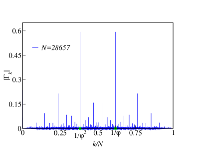
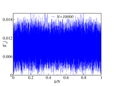
Figure 1: The magnitude of the Fourier transform $\Gamma_{k}$ (Eq. (26)) calculated using the first $N$ terms of the sequence $\{\tau_{i}\}$ as a function of $k/N$ where (top panel) the sequence is taken to be the Fibonacci sequence, and (bottom panel) the sequence is taken to be a typical realization of a random sequence. The number of terms $N$ taken to calculate the Fourier transforms is indicated inside the figure panels.

The difference between a random sequence of $\{\tau_{j}\}=\pm 1$ and the Fibonacci sequence can be easily seen by calculating the Fourier transform of the two sequences defined as

$$\Gamma_{k}~{}=~{}\frac{1}{N}~{}\sum_{j=1}^{N}~{}\tau_{j}~{}\exp\left(\frac{i2\pi k(j-1)}{N}\right),$$ (26)

where the Fourier transform is calculated using the first $N$ terms of the sequence $\{\tau_{j}\}$, and $k=0,1,2,\cdots,N-1$. In Fig. 1 we show the magnitude $|\Gamma_{k}|$ as a function of $k/N$ for (a) the Fibonacci sequence and (b) a typical realization of a random sequence. While the Fourier transform is featureless for the random case, the Fibonacci sequence shows sharp peaks at frequencies that are incommensurate with each other, e.g., the ratio of the frequencies of the two highest peaks equals the golden ratio $\varphi$.

II.5 $P_{\infty}(\cos\theta_{k_{c}},\phi_{k_{c}})$ for p-GGE and ITE

The form of $P_{\infty}(\cos\theta_{k_{c}},\phi_{k_{c}})$ was discussed in Ref. NandySS2017, and the functions have a simple geometric interpretation both for a p-GGE and for an ITE which we will briefly recap here.

For a periodic drive protocol, $U_{k}(T)$ can be written as

$$U_{k}(T)~{}=~{}e^{i\gamma_{k}\hat{e}_{k}\cdot\vec{\sigma}},$$ (27)

where $0\leq\gamma_{k}\leq\pi$, and $\hat{e}_{k}$ is a unit vector with its $x$, $y$, $z$ components denoted by $e_{1k}$, $e_{2k}$, $e_{3k}$ respectively, and $\vec{\sigma}=(\sigma^{x},\sigma^{y},\sigma^{z})$ denote the Pauli matrices. Following the trajectory of a single $k$ mode $|\psi_{k}(n)\rangle$ as a function of $n$ then generates a circle on the Bloch sphere which is defined by the intersection of the unit sphere with a plane that contains the south pole (due to the initial condition $|\psi(0)\rangle$ that we have taken here) and whose normal vector equals $\hat{e}_{k}$. Taking a momentum cell whose width $\delta k$ is small enough such that the variation in $\hat{e}_{k}$ is negligible for the $k$ modes inside the cell, it can then be shown NandySS2017 that the $N_{c}\gg 1$ points (that belong to the consecutive $k$ modes of the coarse-grained cell) on the unit sphere uniformly cover the circle formed by the intersection of this unit sphere with a plane that contains the south pole and whose normal vector equals $\hat{e}_{k_{c}}$. Such a distribution is shown schematically in Fig. 2(a) and arises since $\langle\psi_{k}(n)|\hat{e}_{k}\cdot\vec{\sigma}|\psi_{k}(n)\rangle$ is conserved at each $k$. For a different momentum cell with another average momentum $k_{c}$, the circle on the unit sphere changes due to the change in $\hat{e}_{k_{c}}$ as a function of $k_{c}$. For an ITE, the distribution of the $N_{c}$ points on the unit sphere is even simpler in that these points uniformly cover the surface of the unit sphere independent of $k_{c}$ (shown in Fig. 2(c)). For such a case, following the trajectory of a single $k$ mode $|\psi_{k}(n)\rangle$ as a function of $n$ also covers the unit sphere uniformly when $n$ is large enough. We will show below that for the quasiperiodically driven case, the $N_{c}$ points in a momentum cell form a stable distribution $P_{\infty}(\cos\theta_{k_{c}},\phi_{k_{c}})$ that is neither a circle (Fig. 2(a)) nor a uniform cover (Fig. 2(c)) on the unit sphere surface but is intermediate between these two extreme cases (shown schematically in Fig. 2(b)). In fact, depending on the exact drive parameters (including the form of the drive protocol) and and the value of $k_{c}$, a Fibonacci drive protocol may actually give a wide variety of $P_{\infty}(\cos\theta_{k_{c}},\phi_{k_{c}})$ ranging all the way from Fig. 2(a) to Fig. 2(c). From this geometric viewpoint, it is clear how such a NESS formed due to this quasiperiodic drive protocol is qualitatively different from either a p-GGE or an ITE and allows for much richer possibilities as a function of the drive parameters as we show in the rest of the paper.

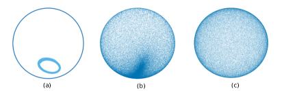
Figure 2: Schematic distribution of the $N_{c}\gg 1$ points in a momentum cell at late times traces out a circle on the surface of the unit sphere for a p-GGE (shown in (a)) and covers the surface of the unit sphere uniformly for an ITE (shown in (c)). For the quasiperiodic Fibonacci drive protocol, the $N_{c}$ points form a stable $P_{\infty}(\cos\theta_{k_{c}},\phi_{k_{c}})$ that is intermediate between (a) and (c), as shown schematically in (b).

III Results for quasiperiodically driven 1D TFIM

III.1 Behaviour of quantities as a function of $n$

We now study the unitary dynamics of the 1D TFIM when $dT\neq 0$ and the $\tau_{i}$’s in Eq. (24) are given by the Fibonacci sequence described in Eq. (25).

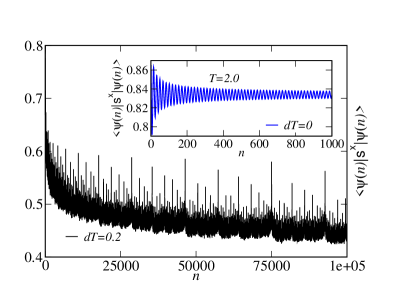
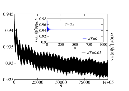
Figure 3: The behaviour of $\langle\psi(n)|s^{x}|\psi(n)\rangle$ as a function of $n$ for the Fibonacci quasiperiodic drive protocol with the parameters $g_{i}=4$, $g_{f}=2$ and $T=2.0$, $dT=0.2$ (top panel), $T=0.2$, $dT=0.05$ (bottom panel). The system size equals $L=4194304$. The inset in both panels shows the behaviour of $\langle\psi(n)|s^{x}|\psi(n)\rangle$ for the perfectly periodic drive with the corresponding value of $T$.

We first study a local quantity, $\langle\psi(n)|s^{x}|\psi(n)\rangle$, as a function of the drive number $n$. This can be straightforwardly calculated in the fermionic representation (Eq. (3)). We show the results for two cases in Fig. 3 where the drive parameters are $g_{i}=4$, $g_{f}=2$, with $T=2.0$ and $dT=0.2$ in the top panel and $T=0.2$, $dT=0.05$ in the bottom panel. The behaviour of this quantity for the same $T$ but with $dT=0$, i.e., a perfectly periodic drive protocol, is also shown in the inset of both panels of Fig. 3. Unlike the periodically driven system where $\langle\psi(n)|s^{x}|\psi(n)\rangle$ approaches a steady state value (described by the corresponding p-GGE and shown in the insets of the top and bottom panels), this local quantity does not seem to approach any well-defined steady state value as a function of $n$ for the quasiperiodically driven system even for $n\sim 10^{5}$ (Fig. 3). Furthermore, $\langle\psi(n)|s^{x}|\psi(n)\rangle$ has cusp-like singularities at multiple values of $n$ (clearly visible in Fig. 3 (top panel) but also present in Fig. 3 (bottom panel)) with the strongest features being present when $n$ equals a Fibonacci number.

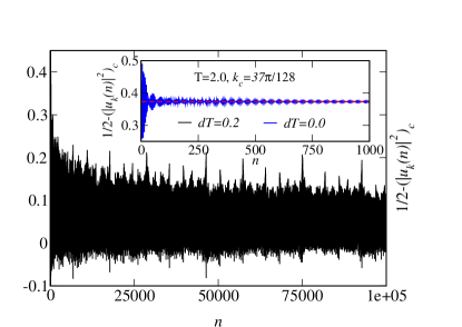
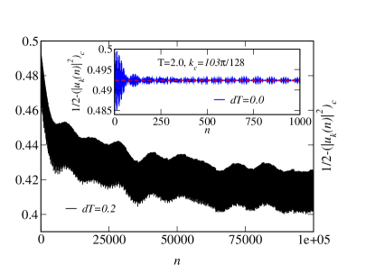
Figure 4: The behaviour of $\left(|u_{k}(n)|^{2}\right)_{c}$ as a function on $n$ for the Fibonacci quasiperiodic drive protocol with the parameters $g_{i}=4$, $g_{f}=2$, $T=2.0$ and $dT=0.2$. The system size equals $L=4194304$ and the $k$ space is divided into $64$ cells with $32768$ consecutive momenta each. The top panel displays the result for $k_{c}=37\pi/128$ and the bottom panel for $k_{c}=103\pi/128$, where $k_{c}$ denotes the average momentum of the corresponding momentum cell. The inset of both panels shows the behaviour of the corresponding quantity for a periodically driven system with $dT=0$. The horizontal red line in both insets indicate the expected steady state value for $dT=0$.

We also show the behaviour of the coarse-grained quantities $(|u_{k}(n)|^{2})_{c}$ defined in Eq. (17) as a function of $n$ for the drive protocol with $T=2.0$ and $dT=0.2$ ($g_{i}=4$, $g_{f}=2$) in Fig. 4. As explained earlier, these quantities approach well-defined steady state values for $n\to\infty$ if a NESS exists. For example, $1/2-(|u_{k}(n)|^{2})_{c}\to 0$ for $n\to\infty$ for any coarse-grained momentum cell if the NESS is an ITE. Similarly, $1/2-(|u_{k}(n)|^{2})_{c}\to\left(\frac{1}{2}\right)e^{2}_{3k_{c}}$ (see Eq. (27)) for a periodically driven system NandySS2017 provided $\delta k$ is small enough so that the variation in $\hat{e}_{k}$ is negligible for the momenta inside a coarse-grained cell. To construct these coarse-grained quantities, we use a system size of $L=4194304$ spins and divide the $k$ space into $64$ momentum cells with each cell containing $32768$ consecutive momenta. In Fig. 4, we show the behaviour of $1/2-(|u_{k}(n)|^{2})_{c}$ as a function of $n$ for $k_{c}=37\pi/128$ (top panel) and $k_{c}=103\pi/128$ (bottom panel), where $k_{c}$ equals the average momentum of a coarse-grained cell in $k$ space. We also show the behaviours of the corresponding quantities for $dT=0$ in the inset of both the panels which show the convergence to the expected values for the periodically driven case. We again see that $(|u_{k}(n)|^{2})_{c}$ does not seem to approach any well-defined steady state value even for $n\sim 10^{5}$ for both the momentum cells. The coarse-grained quantities also have cusp-like features at multiple values of $n$ with the strongest features at values of $n$ that equal any of the Fibonacci numbers, exactly like the local quantity $\langle\psi(n)|s^{x}|\psi(n)\rangle$.

Lastly, we show the trajectory of a single $k$ mode on the corresponding Bloch sphere as a function of $n$ in Fig. 5, where we take $g_{i}=4$, $g_{f}=2$, $T=0.2$ and $dT=0.05$. We see that the trajectory neither follows a circle (as expected for a periodically driven system) nor covers the entire surface of the sphere uniformly (as expected for an ITE) but is a complicated intermediate structure.

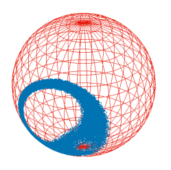
Figure 5: The trajectory of $|\psi_{k}(n)\rangle$ (where $|\psi_{k}(n=0)\rangle=(0,1)^{T}$) for the Fibonacci drive protocol (Eq. (24)) shown on the Bloch sphere. The drive parameters are $g_{i}=4$, $g_{f}=2$, $T=0.2$ and $dT=0.05$. Here $k$ equals $\pi/2$ and the number of drives is taken to be $121393$.

III.2 Behaviour of quantities as a function of $n=F_{m}$

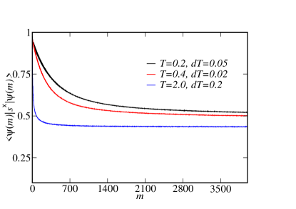
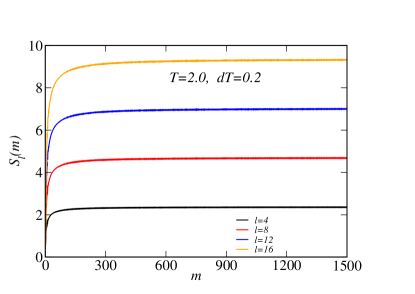
Figure 6: (Top panel) The behaviour of $\langle\psi(n)|s^{x}|\psi(n)\rangle$ as a function of $m$ where the drive number $n=F_{m}$ (we note that $n\sim\varphi^{m}$ for large $m$). (Bottom panel) The behaviour of the entanglement entropy for subsystem sizes $l=4,8,12,16$ as a function of $m$. The system size is $L=4194304$ and $g_{i}=4$ and $g_{f}=2$ for all the cases shown.

From the behaviours of the local quantities shown in Fig. 3 and Fig. 4, it is clear that these do not approach steady state values even for $n\sim 10^{5}$. This is reminiscent of the case studied in Ref. NandySS2017, where the periodically driven system is perturbed with a noise that is scale-invariant in time. The NESS is then only approached after an exponentially long time when the system is viewed not stroboscopically but as $m=2^{n}$ (this was dubbed as a geometric generalized Gibbs ensemble in Ref. NandySS2017, ).

We now use the recursive structure of the Fibonacci sequence to study the unitary dynamics of the system for exponentially long times $n=F_{m}\sim\varphi^{m}$ using only $\mathcal{O}(m)$ unitary matrix multiplications at each $k$. To see this, we simply note that the unitary evolution matrix at level $m$, which we denote by $U_{m}$, equals

$$U_{m+2}~{}=~{}U_{m}U_{m+1},$$ (28)

for all $m\geq 1$ and $U_{1}=U_{k}(T+dT)$, $U_{2}=U_{k}(T-dT)U_{k}(T+dT)$ (see Eq. (25)). We use the recursion level index $m$ (Eq. (25)) as a shorthand to denote $n=F_{m}$. We show results for $\langle\psi(n)|s^{x}|\psi(n)\rangle$ as a function of $m$ for various drive parameters $(T,dT)$ at $g_{i}=4$, $g_{f}=2$ in Fig. 6 (top panel). From these results, it is clear that this local operator does reach a steady state when the system is observed not stroboscopically but at drive numbers $n=F_{m}$. In Fig. 6 (top panel), we see that for some drive parameters ($T=2.0$, $dT=0.2$), the steady state is reached much sooner with $m$ than for the other drive parameters ($T=0.2$, $dT=0.05$ and $T=0.4$, $dT=0.02$). Thus, the value of $\langle\psi(n)|s^{x}|\psi(n)\rangle$ shown in Fig. 3 (bottom panel) for $T=0.2$, $dT=0.05$ up to $n\sim 10^{5}$ is nowhere close to the final steady steady value. While these results strongly suggest a NESS for $l=1$ subsystems, it is also essential to establish the same for other subsystem sizes (where $l\ll L$). To this end, we calculate the entanglement entropy $S_{\mathrm{e}nt}(l)$ (Eq. (16)) for subsystems of size $l=4,8,12,16$ as a function of $n=F_{m}$ and show the results in Fig. 6 (bottom panel) for $T=2.0$ and $dT=0.2$. The entanglement entropy for all the subsystem sizes saturate to well-defined steady state values as a function of $n=F_{m}$ which shows that a NESS (as far as local quantities are concerned) is indeed reached at exponentially long times. We also note that $S_{\mathrm{e}nt}(l)\sim l$ for the steady state values of the entanglement entropy in Fig. 6 (bottom panel) and thus follows a volume law scaling expected for a NESS.

Further evidence for the emergence of a NESS is obtained by looking at the behaviour of the coarse-grained quantities $1/2-(|u_{k}(n)|^{2})_{c}$ for different momentum cells as a function of $n=F_{m}$ instead of stroboscopically (Fig. 7) for the drive parameters $g_{i}=4$, $g_{f}=2$, $T=2.0$ and $dT=0.2$. These coarse-grained quantities also reach a steady state as a function of $n=F_{m}$ with the steady state value being a function of $k_{c}$. Furthermore, the convergence of $(|u_{k}(n)|^{2})_{c}$ to its steady state value is a strong function of $k_{c}$ (Fig. 7) which implies that different local operators have different time scales of approach to their corresponding steady state values.

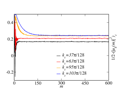
Figure 7: The behaviour of the coarse-grained quantities $1/2-(|u_{k}(n)|^{2})_{c}$ as a function of $m$ where the drive number $n=F_{m}$. The system size is $L=4194304$ and the drive parameters $g_{i}=4$, $g_{f}=2$, $T=2.0$ and $dT=0.2$. The momentum space is divided into $64$ cells with each cell having $32768$ consecutive momentum modes to construct these coarse-grained quantities. $k_{c}$ denotes the average momentum of a coarse-grained cell.

III.3 Behaviour of $\mathcal{P}_{\infty}(\cos\theta_{k_{c}},\phi_{k_{c}})$

To better understand the NESS generated for this quasiperiodic driving protocol when the system is observed not stroboscopically but at $n=F_{m}$, we consider the probability distribution $\mathcal{P}_{n}(\cos\theta_{k_{c}},\phi_{k_{c}})$ generated by the motion of the $N_{c}\gg 1$ points on the unit sphere for each coarse-grained momentum cell (with average momentum $k_{c}$) as a function of $n=F_{m}$. To do this numerically, we consider $L=16777216$ and divide the momentum space into $32$ cells with each coarse-grained cell having $262144$ consecutive momentum modes. Here we show the evolution of $\mathcal{P}_{n}(\cos\theta_{k_{c}},\phi_{k_{c}})$ as a function of $n=F_{m}$ for two drive protocols with $g_{i}=4$, $g_{f}=2$, $T=0.2$ and $T=0.05$ (Fig. 8) and with $g_{i}=4$, $g_{f}=2$, $T=2.0$ and $T=0.2$ (Fig. 9). The momentum cell chosen has an average momentum of $k_{c}=31\pi/64$ in the former case and $k_{c}=19\pi/64$ in the latter case. In both the cases, the $N_{c}$ points start from the south pole of the unit sphere at $n=0$ due to the choice of $|\psi(n=0)\rangle$ taken here.

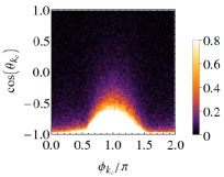
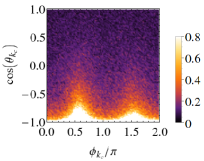
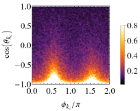
Figure 8: The evolution of $\mathcal{P}_{n}(\cos\theta_{k_{c}},\phi_{k_{c}})$ as a function of $n=F_{m}$ for a coarse-grained momentum cell with $N_{c}=262144$ consecutive momenta and $k_{c}=31\pi/64$. The drive parameters are $g_{i}=4$, $g_{f}=2$, $T=0.2$ and $T=0.05$. $m$ takes the value $100$ (top left), $300$ (top right), $1000$ (bottom left), $2000$ (bottom right) in the four panels.

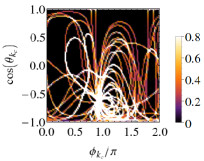
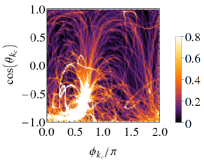
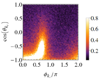
Figure 9: The evolution of $\mathcal{P}_{n}(\cos\theta_{k_{c}},\phi_{k_{c}})$ as a function of $n=F_{m}$ for a coarse-grained momentum cell with $N_{c}=131072$ consecutive momenta and $k_{c}=19\pi/64$. The drive parameters are $g_{i}=4$, $g_{f}=2$, $T=2.0$ and $T=0.2$. Here $F_{1}=1$, $F_{2}=2$ and $F_{m}=F_{m-1}+F_{m-2}$ for $m>2$ with $F_{m}\sim\varphi^{m}$ for large $m$. $m$ takes the value $15$ (top left), $20$ (top right), $50$ (bottom left), $100$ (bottom right) in the four panels.

From the results presented in Fig. 8 and Fig. 9, we clearly see that $\mathcal{P}_{n}(\cos\theta_{k_{c}},\phi_{k_{c}})$ does have a well-defined long time limit $\mathcal{P}_{\infty}(\cos\theta_{k_{c}},\phi_{k_{c}})$ when the system is observed at $n=F_{m}$. The rate of convergence to $\mathcal{P}_{\infty}(\cos\theta_{k_{c}},\phi_{k_{c}})$ again depends on the details of the drive protocol and on $k_{c}$. Most importantly, $\mathcal{P}_{\infty}(\cos\theta_{k_{c}},\phi_{k_{c}})$ is neither a circle on the unit sphere as is expected for a p-GGE (or, a g-GGE NandySS2017 ) nor a uniform cover of its surface as is the case for an ITE NandySS2017 but rather something intermediate as shown schematically in Fig. 2. As can be seen from Fig. 8 and Fig. 9, the exact form of $\mathcal{P}_{\infty}(\cos\theta_{k_{c}},\phi_{k_{c}})$ is a function of the drive parameters and $k_{c}$ which suggests that the exact form of the NESS can be tuned by changing these parameters appropriately.

III.4 KKT invariant for the Fibonacci sequence

Given any two SU(2) matrices $U_{1}$ and $U_{2}$, a Fibonacci sequence of matrices is defined by the recursion relation shown in Eq. (28). Let us parametrize $U_{m}$ as

$$U_{m}~{}=~{}e^{i\theta_{m}\hat{n}_{m}\cdot\vec{\sigma}},$$ (29)

where $0\leq\theta_{m}\leq\pi$ and $\hat{n}_{m}$ is a unit vector. We also define

$$\Gamma_{m,m+1}~{}=~{}\cos^{-1}(\hat{n}_{m}\cdot\hat{n}_{m+1}),$$ (30)

where $0\leq\Gamma_{m,m+1}\leq\pi$. It was shown by Kohmoto, Kadanoff and Tang (Ref. KohmotoKT1983, ) and Sutherland (Ref. Sutherland1986, ) that a quantity defined as

$$I_{s}~{}=~{}-~{}(\sin\theta_{m}~{}\sin\theta_{m+1}~{}\sin\Gamma_{m,m+1})^{2}$$ (31)

is independent of $m$; we will call this the KKT invariant henceforth. This places a simple constraint on the allowed values of $\theta_{m}$ since from Eq. (30), we have

$$\sin\theta_{m}~{}=~{}\frac{\sqrt{|I_{s}|}}{\sin\theta_{m+1}\sin\Gamma_{m,m+1}}~{}\geq~{}\sqrt{|I_{s}|}.$$ (32)

In Fig. 10 (top panel), we show that this constraint is indeed satisfied in our numerics for any $k$ mode when the unitary evolution matrix is calculated at $n=F_{m}$. The KKT invariant $I_{s}$ is strongly dependent on $k$ and $dT$ for a fixed set of values of $g_{i}$, $g_{f}$ and $T$ as can be seen from Fig. 10 (bottom panel). The strong dependence of $I_{s}$ on the drive parameters and momentum $k$ makes the dependence of $\mathcal{P}_{\infty}(\cos\theta_{k_{c}},\phi_{k_{c}})$ on the drive parameters and $k_{c}$ plausible. In particular, if $I_{s}$ is close to $-1$, then the allowed values of $\theta_{m}$ are strongly constrained. We should stress here that the constraint on $\theta_{m}$ does not imply that the motion of the state $|\psi_{k}\rangle$ generated by $U_{m}$ necessarily has forbidden regions on the Bloch sphere (however, see the next section).

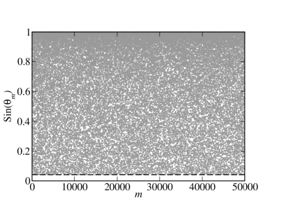
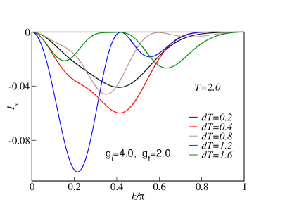
Figure 10: (Top panel) The evolution of $\sin\theta_{m}$ as a function of $m$ for the Fibonacci sequence defined in Eq. (28) for a mode with $k=2\pi/5$, and $g_{i}=4$, $g_{f}=2$, $T=2.0$ and $dT=1.2$. With these parameters, $I_{s}\approx-0.0016877$. (Bottom panel) The KKT invariant $I_{s}$ as a function of $k$ for a fixed $g_{i}=4$, $g_{f}=2$, $T=2.0$, and different values of $dT$.

IV Analysis of a toy problem

In this section, instead of taking $U_{1}=U_{k}(T+dT)$ and $U_{2}=U_{k}(T-dT)U_{k}(T+dT)$ in Eq. (28), we will consider a simpler problem of a single two-level system with the following initial matrices $U_{1}$ and $U_{2}$,

$$U_{1} = e^{-i\sigma_{z}\left(\frac{\pi}{2}+\epsilon\right)},$$

$$U_{2} = e^{-i\sigma_{x}\left(\frac{\pi}{2}+\epsilon\right)},$$ (33)

and follow the motion of a state $|\psi\rangle=(0,1)^{T}$ on the Bloch sphere under the action of $U_{m}$ (generated by the recursion in Eq. (28)) as a function of $m$. For $\epsilon=0$, $U_{m}$ for any $m$ will be of the form $\pm e^{-i\sigma_{a}\left(\pi/2\right)}$ where $a=x,y,z$. Thus the state $|\psi\rangle$, when represented on the Bloch sphere, will equal one of the eight points $(0,0,\pm 1),(0,\pm 1,0),(\pm 1,0,0)$ as a function of $m$.

When $\epsilon\neq 0$, the problem is no longer analytically tractable and requires a numerical analysis. We show the result of such an analysis in Fig. 11 where the trajectory of the state $|\psi\rangle$ on the surface of the Bloch sphere is shown for four different values of $\epsilon$ for a large value of $m=10^{6}$. We see that for $\epsilon=0.10$ (top left panel, Fig. 11) and $\epsilon=0.28$ (top right panel, Fig. 11), there are still forbidden regions on the Bloch sphere just like the case of $\epsilon=0$. However, for larger values of $\epsilon$ like $\epsilon=0.29$ (bottom left panel, Fig. 11) and $\epsilon=0.40$ (bottom right panel, Fig. 11), the trajectory seems to completely fill the surface of the sphere, though in a highly non-uniform manner. This simple toy problem thus illustrates the richness of possible structures that can emerge for suitable choices of the matrices $U_{1}$ and $U_{2}$ which may be controlled by choosing the exact nature of $g_{\mathrm{ref}}(t)$ and the momentum $k$.

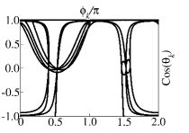
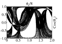
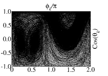
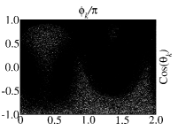
Figure 11: The trajectory of a state $|\psi\rangle$ as a function of $m$ on the surface of the (unit) Bloch sphere for $m=10^{6}$. The Fibonacci sequence of matrices $U_{m}$ is defined by the sequence Eq. (28) and $U_{1},U_{2}$ have the forms shown in Eq. (33). The values of $\epsilon$ used in the different panels are $\epsilon=0.10$ (top left), $\epsilon=0.28$ (top right), $\epsilon=0.29$ (bottom left) and $\epsilon=0.40$ (bottom right).

We now analyze the Fibonacci sequence in the limit that the KKT invariant $I_{s}\to-1$ to understand some features of the above problem when $\epsilon$ is small. To simplify the notation, let us start at some value of $m$ and define

$$\theta_{m} \equiv \frac{\pi}{2}~{}+~{}\epsilon_{1},$$

$$\theta_{m+1} \equiv \frac{\pi}{2}~{}+~{}\epsilon_{2},$$

$$\Gamma_{m,m+1} \equiv \frac{\pi}{2}~{}+~{}\gamma,$$ (34)

where $\theta_{m}$ and $\Gamma_{m,m+1}$ are defined in Eqs. (29-30). Then $I_{s}$ close to $-1$ implies that $\epsilon_{1}$, $\epsilon_{2}$ and $\gamma$ all lie close to zero. An alternate way of writing Eq. (34) is

$$\sin\epsilon_{1} = -~{}\frac{1}{2}\mathrm{tr}(U_{m}),$$

$$\sin\epsilon_{2} = -~{}\frac{1}{2}\mathrm{tr}(U_{m+1}),$$

$$\sin\gamma = -~{}\hat{n}_{m}\cdot\hat{n}_{m+1}.$$ (35)

The KKT invariant is then given by

$$I_{s}~{}=~{}-1~{}+~{}\epsilon_{1}^{2}~{}+~{}\epsilon_{2}^{2}~{}+~{}\gamma^{2}$$ (36)

plus terms of fourth order in $\epsilon_{1},~{}\epsilon_{2},~{}\gamma$. We then find from the recursion relation in Eq. (28) that, to third order in the small parameters $\epsilon_{1},~{}\epsilon_{2},~{}\gamma$, the quantities defined in Eq. (34) for $m$ transform as follows when $m\to m+1$:

$$\epsilon_{1} \to \epsilon_{2},$$

$$\epsilon_{2} \to -~{}\gamma~{}-~{}\epsilon_{1}\epsilon_{2}~{}+~{}\frac{1}{2}~{}\gamma~{}(\epsilon_{1}^{2}~{}+~{}\epsilon_{2}^{2}),$$

$$\gamma \to \epsilon_{1}~{}-~{}\epsilon_{2}\gamma~{}+~{}\frac{1}{2}~{}\epsilon_{1}~{}(\gamma^{2}~{}-~{}\epsilon_{2}^{2}).$$ (37)

Iterating Eqs. (37) six times, we find that when $m\to m+6$,

$$\epsilon_{1} \to \epsilon_{1}~{}+~{}4\epsilon_{1}~{}(\gamma^{2}-\epsilon_{2}^{2}),$$

$$\epsilon_{2} \to \epsilon_{2}~{}+~{}4\epsilon_{2}~{}(\epsilon_{1}^{2}-\gamma^{2}),$$

$$\gamma \to \gamma~{}+~{}4\gamma~{}(\epsilon_{2}^{2}-\epsilon_{1}^{2}).$$ (38)

Since $\epsilon_{1},~{}\epsilon_{2},~{}\gamma$ are small, the changes in these parameters given in Eqs. (38) are small. It is then convenient to replace those equations by differential equations where we define

$$\frac{dz}{dm}~{}\equiv~{}\frac{z(m+6)~{}-~{}z(m)}{6},$$ (39)

where $z$ can denote any of the variables given in Eqs. (38). We then obtain the equations

$$\frac{d\epsilon_{1}}{dm} = \frac{2}{3}~{}\epsilon_{1}~{}(\gamma^{2}-\epsilon_{2}^{2}),$$

$$\frac{d\epsilon_{2}}{dm} = \frac{2}{3}~{}\epsilon_{2}~{}(\epsilon_{1}^{2}-\gamma^{2}),$$

$$\frac{d\gamma}{dm} = \frac{2}{3}~{}\gamma~{}(\epsilon_{2}^{2}-\epsilon_{1}^{2}).$$ (40)

We observe that Eqs. (40) conserve the invariant $I_{s}$ given in Eq. (36); this implies that a point with the coordinates $(\epsilon_{1},\epsilon_{2},\gamma)$ moves on the surface of a sphere. Interestingly, Eqs. (40) conserve another quantity $C$ given by

$$C~{}=~{}\epsilon_{1}\epsilon_{2}\gamma.$$ (41)

The presence of this invariant implies that the point $(\epsilon_{1},\epsilon_{2},\gamma)$ moves on closed curves on the surface of the sphere, so that we have effectively only one quantity which changes with $m$. We thus have an integrable system to this order in $\epsilon_{1},~{}\epsilon_{2},~{}\gamma$. [We note from Eq. (34) that $C=-\cos(\theta_{m})\cos(\theta_{m+1})\cos(\Gamma_{m,m+1})$ to third order in $\epsilon_{1},~{}\epsilon_{2},~{}\gamma$. We will plot the latter quantity in Fig. 12 below since it is easier to calculate numerically].

We will now apply the above analysis to the case defined in Eq. (33). The initial conditions are then given by

$$\epsilon_{1} = \epsilon_{2}~{}=~{}\epsilon,~{}~{}~{}~{}\gamma~{}=~{}0.$$ (42)

Eqs. (40) then simplify to

$$\frac{d\epsilon_{1}}{dm} = -\frac{2}{3}~{}\epsilon_{1}\epsilon_{2}^{2},$$

$$\frac{d\epsilon_{2}}{dm} = \frac{2}{3}~{}\epsilon_{1}^{2}\epsilon_{2}.$$ (43)

Since $\epsilon_{1}^{2}+\epsilon_{2}^{2}=2\epsilon^{2}$ is an invariant, we can parametrize

$$\epsilon_{1}~{}=~{}\sqrt{2}\epsilon\sin\phi~{}~{}~{}{\rm and}~{}~{}~{}\epsilon_{2}~{}=~{}\sqrt{2}\epsilon\cos\phi.$$ (44)

Eqs. (43) imply that

$$\frac{d\phi}{dm}~{}=~{}-\frac{2}{3}~{}\epsilon^{2}\sin\phi\cos\phi.$$ (45)

This equation has stable fixed points at $\phi=0$ and $\pi$, and unstable fixed points at $\phi=\pi/2$ and $3\pi/2$. At $m=0$, the initial condition (Eq. (42)) fixes $\phi=\pi/4$. Eq. (45) then implies that $\phi$ will flow to zero as $m$ increases, so that $\epsilon_{1}\to 0$ and $\epsilon_{2}\to\sqrt{2}\epsilon$. According to Eq. (45), the time scale (here we are thinking of $m$ as time) of approaching the fixed point should be of the order of $1/\epsilon^{2}$. According to the first order terms in Eq. (37), $\epsilon_{1}$ cycles as $\epsilon_{1}\to\epsilon_{2}\to-\gamma\to-\epsilon_{1}\to-\epsilon_{2}\to\gamma\to\epsilon_{1}$ for six successive iterations. Hence $\sin\theta_{m}=\cos\epsilon_{1}$ should cycle over three different values given by $1-\epsilon_{1}^{2}/2,~{}1-\epsilon_{2}^{2}/2,~{}1-\gamma^{2}/2$. Monitoring $\sin\theta_{m}=\cos\epsilon_{1}\approx 1-\epsilon_{1}^{2}/2$ for $\epsilon=0.1$ as a function of $m$ (Fig. 12) clearly shows that $\epsilon_{1},\epsilon_{2},\gamma$ do not remain at one particular fixed point permanently; after long intervals of time, they move from one fixed point to another relatively quickly. For example, for $\epsilon=0.1$, this movement happens at intervals of about $m=3200$; the movement itself occurs over a duration of $m=100$ (which is equal to $1/\epsilon^{2}$). We will argue below that these movements may be understood qualitatively by appealing to terms higher than third order which we have ignored when deriving Eqs. (40).

We will begin by finding the fixed points of Eqs. (40). The KKT invariant implies that the three parameters lie on the surface of a sphere

$$\epsilon_{1}^{2}~{}+~{}\epsilon_{2}^{2}~{}+~{}\gamma^{2}~{}=~{}r^{2},$$ (46)

where $r$ is a small number. We then find that there are two types of fixed points.

(i) Any two of the parameters $\epsilon_{1},~{}\epsilon_{2},~{}\gamma$ are equal to zero, and the third one is equal to $\pm r$. This gives six possible fixed points.

(ii) $\epsilon_{1}^{2}=\epsilon_{2}^{2}=\gamma^{2}=r^{2}/3$. This gives eight possible fixed points.

Next, we look at the stability of the above fixed points. Denoting the first order deviations of the three parameters from a fixed point by $\delta_{i}$ (where $i=1,2,3$), we obtain equations of the form

$$\frac{d\delta_{i}}{dm}~{}=~{}\sum_{j=1}^{3}~{}M_{ij}\delta_{j}.$$ (47)

The eigenvalues of the matrix $M$ determine the stability of a fixed point; if any one of the eigenvalues has a positive real part, the fixed point is unstable. For the six fixed points of type (i), the eigenvalues turn out to be 0 and $\pm(2/3)r^{2}$, implying that each of these fixed points is unstable along some direction. For the eight fixed points of type (ii), the eigenvalues are 0 and $\pm i(2/3\sqrt{3})r^{2}$; hence a small deviation from these fixed points will oscillate but not grow with time.

The invariant $C=\epsilon_{1}\epsilon_{2}\gamma$ defined in Eq. (41) is equal to 0 for the fixed points of type (i) and $\pm r^{3}/(3\sqrt{3})$ for the fixed points of type (ii). For the cases studied numerically, i.e., $(\epsilon_{1},\epsilon_{2},\gamma)=(\epsilon,\epsilon,0)$ at $m=0$, we have $r=\sqrt{2}\epsilon$ and $C=0$. For this case, we have seen above that the systems flows to the fixed point $(0,\sqrt{2}\epsilon,0)$ over a time scale of order $1/\epsilon^{2}$. However, this is an unstable fixed point; hence even a small deviation from this fixed point in an unstable direction will grow exponentially with $m$.

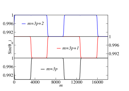
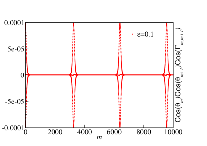
Figure 12: (Top panel) The evolution of $\sin\theta_{m}$ as a function of $m$ for $\epsilon=0.1$. (Bottom panel) The evolution of $\cos\theta_{m}\cos\theta_{m+1}\cos\Gamma_{m,m+1}$ as a function of $m$ for $\epsilon=0.1$.

We now note that while the KKT invariant is an exact invariant, the quantity $C$ defined in Eq. (41) is invariant only up to terms of third order in $\epsilon_{1},~{}\epsilon_{2},~{}\gamma$. Considering the possible effects of terms of higher than third order on the right hand sides of Eqs. (40), we may expect that over very long periods of time (i.e., periods which are much larger than $1/\epsilon^{2}$), the three parameters will differ from what we would obtain if only the third order terms were present in Eqs. (40). As a result, we would also expect $C$ to deviate eventually from its initial value, i.e., from $C=0$. We therefore expect that over long times, $|C|$ will not exactly be equal to zero, although it will remain much smaller than the largest possible value of $r^{3}/(3\sqrt{3})\simeq 0.00054$. Fig. 12 confirms this numerically for the case $\epsilon=0.1$ where we monitor $\cos\theta_{m}\cos\theta_{m+1}\cos\Gamma_{m,m+1}$ which is equal to $-C$ for small $\epsilon_{1},\epsilon_{2},\gamma$.

Given that $C$ is very small but not exactly equal to zero, we can now see how the parameters $\epsilon_{1},~{}\epsilon_{2},~{}\gamma$ will change over very long periods of time. In the beginning, when $\gamma$ is very close to zero, we have seen that $\epsilon_{1}$ flows to zero while $\epsilon_{2}$ flows to $\sqrt{2}\epsilon$; these flows occur over a time scale of order $1/\epsilon^{2}=100$. According to Eqs. (40), this is a stable fixed point for $\epsilon_{1}$ but not for $\gamma$. Eventually, therefore, $\gamma$ will start growing while $\epsilon_{1}$ will remain small. Once $\gamma$ becomes larger than $\epsilon_{1}$, $\epsilon_{2}$ will start becoming smaller. Thus the behaviors of $\epsilon_{1},~{}\epsilon_{2},~{}\gamma$ will get cyclically interchanged; namely, $\epsilon_{1}$ will stay very close to zero, $\epsilon_{2}$ will flow to zero and $\gamma$ will flow to $\sqrt{2}\epsilon$. Eventually, this behavior again gets interchanged; $\epsilon_{2}$ stays very close to zero while $\gamma$ and $\epsilon_{1}$ flow to zero and $\sqrt{2}\epsilon$ respectively. This is indicated in Fig. 12 where we see that out of the three quantities $1-\epsilon_{1}^{2}/2$, $1-\epsilon_{2}^{2}/2$, and $1-\gamma^{2}/2$, two of them remain close to one while the third one remains close to $1-\epsilon^{2}=0.99$ at all times (except for some rapid changes occurring over a time scale of order $1/\epsilon^{2}$). We see that this behavior gets cyclically interchanged after time intervals of the order of 3200. We cannot quantitatively explain the value 3200 since we do not know the form of the higher order terms that will appear on the right hand sides of Eqs. (40); however, as argued above, we do expect this time scale to be much larger than $1/\epsilon^{2}=100$.

V Conclusions and outlook

In this work, we have considered a prototypical many-body integrable model, the one-dimensional transverse field Ising model, that is continually driven by a time-dependent magnetic field resulting in a unitary dynamics. The translational symmetry of the system allows for a mapping to a pseudospin representation for each momentum $k$, where the pseudospin is driven by its own time-dependent pseudo-magnetic field that varies with $k$ (Eq. (8)). In the thermodynamic limit, for a subsystem whose size is much smaller than that of the total system, the reduced density matrix of the subsystem is fixed by certain coarse-grained quantities in momentum space (Eq. (17)). These coarse-grained quantities have a well-defined large $n$ limit in case a nonequilibrium steady state exists at late times. We also define a probability distribution on the unit sphere for each value of average $k_{c}$ by using a large number of consecutive momenta in a small cell that is centered around $k_{c}$ and using the pseudospin representation for each $k$ to represent the corresponding state on the unit sphere. This probability distribution for each $k_{c}$ changes in an irreversible manner and approaches a steady state distribution in the limit $n\to\infty$.

We consider a driving protocol with two types of square pulses with possible periods $T+dT$ and $T-dT$ such that the unitary time evolution operators $U_{k}(T+dT)$ and $U_{k}(T-dT)$ do not commute with each other. These pulses alternate according to a Fibonacci sequence to mimic a quasiperiodic drive that is neither periodic nor random in time. We find that neither the local quantities nor the coarse-grained quantities approach a well-defined steady state if the system is viewed stroboscopically for even $n\sim 10^{5}$. However, when the system is viewed at $n=F_{m}$ (where $F_{m}$ are the Fibonacci numbers which increase as $\varphi^{m}$ for large $m$), a well-defined nonequilibrium steady state indeed emerges at exponentially late times. This exponentially late approach to the steady state was also previously found by us for another driving protocol that was neither random nor periodic NandySS2017 . We believe that this may be a generic feature of quasiperiodically driven integrable systems.

To characterize the nonequilibrium steady state, we also look at the probability distribution of consecutive momenta in a momentum cell centered at $k_{c}$. We find that the final probability distribution is qualitatively different compared to the distributions that arise for a periodically driven system or a system that locally heats up to an infinite temperature ensemble, i.e., it is neither a circle nor a uniform covering of the unit sphere. Furthermore, the form of the distribution is sensitive to the parameters of the driving protocol and the value of $k_{c}$. We also study a toy problem of a single two-level system where the unitary matrices are arranged in a Fibonacci sequence to illustrate how the nature of the distribution on the Bloch sphere is highly sensitive to the parameters of the problem. In the limit where the KKT invariant is close to $-1$, the problem can be studied analytically to a large extent, and we find an intricate pattern for the state at late times.

A deeper understanding of these distributions and their tunability with the drive parameters and $k_{c}$ is highly desirable since that would lead to a wide variety of nonequilibrium steady states that were previously unknown. Another open question is to come up with a simple ensemble description for the resulting steady state since it lies beyond a periodic generalized Gibbs ensemble approach. Finally, we note that the one-dimensional transverse field Ising model driven by a Fibonacci sequence of square pulses has been recently studied in the high frequency limit, and it has been shown that a nonequilibrium steady state emerges in that limit which resembles the steady state of a periodically driven system Maity2018 .

References

- (1) I. Bloch, “Ultracold quantum gases in optical lattices”, Nature Physics, 1, 23 (2005).
- (2) A. Polkovnikov, K. Sengupta, A. Silva, and M. Vengalattore, “Colloquium: Nonequilibrium dynamics of closed interacting quantum systems”, Rev. Mod. Phys. 83, 863 (2011).
- (3) N. Goldman and J. Dalibard, “Periodically Driven Quantum Systems: Effective Hamiltonians and Engineered Gauge Fields”, Phys. Rev. X 4, 031027 (2014).
- (4) T. Langen, R. Geiger, and J. Schmiedmayer, “Ultracold Atoms Out of Equilibrium”, Annu. Rev. Condens. Matter Phys. 6, 201 (2015).
- (5) A. Eckardt, “Colloquium: Atomic quantum gases in periodically driven optical lattices”, Rev. Mod. Phys. 89, 011004 (2017).
- (6) D. V. Else, B. Bauer, and C. Nayak, “Floquet Time Crystals”, Phys. Rev. Lett. 117, 090402 (2016).
- (7) V. Khemani, A. Lazarides, R. Moessner, and S. L. Sondhi, “On the phase structure of driven quantum systems”, Phys. Rev. Lett. 116, 250401 (2016).
- (8) R. Moessner and S. L. Sondhi, “Equilibration and order in quantum Floquet matter”, Nat. Phys. 13, 424 (2017).
- (9) M. Kollar, F. A. Wolf, and M. Eckstein, “Generalized Gibbs ensemble prediction of prethermalization plateaus and their relation to nonthermal steady states in integrable systems”, Phys. Rev. B 84, 054304 (2011).
- (10) A. Lazarides, A. Das, and R. Moessner, “Periodic Thermodynamics of Isolated Quantum Systems”, Phys. Rev. Lett. 112, 150401 (2014).
- (11) A. Lazarides, A. Das, and R. Moessner, “Equilibrium states of generic quantum systems subject to periodic driving”, Phys. Rev. E 90, 012110 (2014).
- (12) P. Ponte, A. Chandran, Z. Papić, and D. A. Abanin, “Periodically driven ergodic and many-body localized quantum systems”, Annals of Physics 353, 196 (2015).
- (13) L. D’Alessio and M. Rigol, “Long-time Behavior of Isolated Periodically Driven Interacting Lattice Systems”, Phys. Rev. X 4, 041048 (2014).
- (14) E. T. Jaynes, “Information Theory and Statistical Mechanics”, Phys. Rev. 106, 620 (1957).
- (15) E. T. Jaynes, “Information Theory and Statistical Mechanics. II”, Phys. Rev. 108, 171 (1957).
- (16) R. Nandkishore and D. A. Huse, “Many body localization and thermalization in quantum statistical mechanics”, Annu. Rev. Condens. Matter Phys. 6, 15 (2015).
- (17) T. Kitagawa, E. Berg, M. Rudner, and E. Demler, “Topological characterization of periodically driven systems”, Phys. Rev. B 82, 235114 (2010).
- (18) A. Russomanno, A. Silva, and G. E. Santoro, “Periodic Steady Regime and Interference in a Periodically Driven Quantum System”, Phys. Rev. Lett. 109, 257201 (2012).
- (19) M. Bukov, L. D’Alessio, and A. Polkovnikov, “Universal high-frequency behavior of periodically driven systems: from dynamical stabilization to Floquet engineering”, Advances in Physics 64, 139 (2015).
- (20) P. Ponte, Z. Papić, F. Huveneers, and D. A. Abanin, “Many-Body Localization in Periodically Driven Systems”, Phys. Rev. Lett. 114, 140401 (2015).
- (21) A. Eckardt and E. Anisimovas, ”High-frequency approximation for periodically driven quantum systems from a Floquet-space perspective”, New J. Phys. 17, 093039 (2015).
- (22) S. Sachdev, Quantum Phase Transitions (Cambridge University Press, Cambridge, 2011).
- (23) A. Dutta, G. Aeppli, B. K. Chakrabarti, U. Divakaran, T. F. Rosenbaum, and D. Sen, Quantum phase transitions in transverse field spin models: from statistical physics to quantum information (Cambridge University Press, Cambridge, 2015).
- (24) X.-Y. Feng, G.-M. Zhang, and T. Xiang, “Topological Characterization of Quantum Phase Transitions in a Spin- Model”, Phys. Rev. Lett. 98, 087204 (2007).
- (25) H.-D. Chen and Z. Nussinov, “Exact results on the Kitaev model on a hexagonal lattice: spin states, string and brane correlators, and anyonic excitations”, J. Phys. A: Math. Theor. 41, 075001 (2008).
- (26) V. Mukherjee, A. Dutta, and D. Sen, “Defect generation in a spin-1/2 transverse chain under repeated quenching of the transverse field”, Phys. Rev. B 77, 214427 (2008).
- (27) A. Das, “Exotic freezing of response in a quantum many-body system”, Phys. Rev. B 82, 172402 (2010).
- (28) A. Dutta, A. Das, and K. Sengupta, “Statistics of work distribution in periodically driven closed quantum systems”, Phys. Rev. E 92, 012104 (2015).
- (29) A. Sen, S. Nandy, and K. Sengupta, “Entanglement generation in periodically driven integrable systems: Dynamical phase transitions and steady state”, Phys. Rev. B 94, 214301 (2016).
- (30) S. Nandy, K. Sengupta, and A. Sen, “Periodically driven integrable systems with long-range pair potentials”, J. Phys. A: Math. Theor. 51, 334002 (2018).
- (31) J. Marino and A. Silva, “Relaxation, prethermalization, and diffusion in a noisy quantum Ising chain”, Phys. Rev. B 86, 060408 (R) (2012).
- (32) G. Roósz, R. Juhász, and F. Iglói, “Nonequilibrium dynamics of the Ising chain in a fluctuating transverse field”, Phys. Rev. B 93, 134305 (2016).
- (33) S. Nandy, A. Sen, and D. Sen, “Aperiodically Driven Integrable Systems and Their Emergent Steady States”, Phys. Rev. X 7, 031034 (2017).
- (34) H.-H. Lai and K. Yang, “Entanglement entropy scaling laws and eigenstate typicality in free fermion systems”, Phys. Rev. B 91, 081110 (2015).
- (35) S. Nandy, A. Sen, A. Das, and A. Dhar, “Eigenstate Gibbs ensemble in integrable quantum systems”, Phys. Rev. B 94, 245131 (2016).
- (36) M. Kohmoto, L. P. Kadanoff, and C. Tang, “Localization Problem in One Dimension: Mapping and Escape”, Phys. Rev. Lett. 50, 1870 (1983).
- (37) B. Sutherland, “Simple System with Quasiperiodic Dynamics: a Spin in a Magnetic Field”, Phys. Rev. Lett. 57, 770 (1986).
- (38) E. Lieb, T. Schultz, and D. Mattis, “Two soluble models of an antiferromagnetic chain”, Ann. Phys. (N.Y.) 16, 407 (1961).
- (39) M. Kolodrubetz, B. K. Clark, and D. A. Huse, “Nonequilibrium Dynamic Critical Scaling of the Quantum Ising Chain”, Phys. Rev. Lett. 109, 015701 (2012).
- (40) G. Vidal, J. I. Latorre, E. Rico, and A. Kitaev, “Entanglement in Quantum Critical Phenomena”, Phys. Rev. Lett. 90, 227902 (2003).
- (41) I. Peschel, “Calculation of reduced density matrices from correlation functions”, J. Phys. A: Math. Gen. 36, L205 (2003).
- (42) A. Thue, “Über unendliche Zeichenreihen”, Norske Vididensk. Selsk. Skr. I. 7, 1 (1906).
- (43) M. Morse, “Recurrent geodesics on a surface of negative curvature”, Trans. Am. Math. Soc. 22, 84 (1921).
- (44) M. Morse, “A One-to-One Representation of Geodesics on a Surface of a Negative Curvature”, Am. J. Math. 43, 35 (1921).
- (45) M. Schroeder, Fractals, Chaos, Power Laws: Minutes from an Infinite Paradise (W.H. Freeman and Company, New York, 1991).
- (46) S. Maity, U. Bhattacharya, A. Dutta and D. Sen, “Fibonacci steady states in a driven integrable quantum system”, arXiv:1810.03114.