How production networks amplify economic growth

Abstract

Technological improvement is the most important cause of long-term economic growth. We study the effects of technology improvement in the setting of a production network, in which each producer buys input goods and converts them to other goods, selling the product to households or other producers. We show how this network amplifies the effects of technological improvements as they propagate along chains of production. Longer production chains for an industry bias it towards faster price reduction, and longer production chains for a country bias it towards faster GDP growth. These predictions are in good agreement with data and improve with the passage of time, demonstrating a key influence of production chains in price change and output growth over the long term.

I Introduction

Economic output is the result of a network of industries that buy goods from one another, convert them to new goods, and sell the output to households or other industries. Since work by Leontief [1, 2] increasingly rich data have become available to study these networks, and research has revealed characteristics that hold across diverse economies, such as their link weight and industry size distributions [3, 4, 5, 6, 7], community structure [6], and path-length properties [8]. Economies typically have a few highly central industries that are strong suppliers to the rest of the network [7, 9, 5], a feature that has been incorporated into models where short-term fluctuations in output are generated by shocks to individual industries [10, 7, 11, 12, 13, 14].

In this paper we study how the network structure of production affects an economy’s long-term growth. Our argument proceeds in two steps. First we show that the rate of change of an industry’s price is a function of its position in the production network. This happens because productivity improvements accumulate along supply chains. As a result, industries that rely on longer supply chains experience stronger price declines than others. Second, we show how this observation can help explain cross-country differences in economic growth. Because an industry’s position in the production network and the industrial composition of a country are slow-moving variables, aggregate growth can be predicted from the structure of a country’s production network. Intuitively, countries whose final demand relies relatively more on industries with longer supply chains should grow more quickly. We find that detailed observations across industries and countries are consistent with both predictions, and help explain why some countries grow faster than others.

A large literature stresses that technological improvements are the main driver of long-term growth [15, 16]. Over time, improvements to productivity – the amount of output that can be made with a given amount of inputs – significantly alter prices and production flows in an economy. Classic work by Domar [17] and Hulten [18] showed that as an industry’s productivity improves, the presence of intermediate input trade – i.e. goods and services flowing through a production network – amplifies the aggregate benefit for an economy. Productivity growth in an industry not only reduces the price and raises the output of its goods, but some of this output can be used as inputs by other industries, enabling further increases in output, and so on.

However, other predictions about the role of production networks have escaped notice. Using a simple model, we show that as the effects of productivity changes propagate, each industry’s price declines at a rate that depends on its network position. An industry’s price should fall in proportion to its output multiplier, a centrality metric that can be understood as the average length of an industry’s production chains where every production path is weighted by the relative size of the expenditures it represents. An industry benefits from both its own productivity growth and from the accumulation of productivity improvements in its upstream suppliers. As a result, the longer its chains of production, the faster its expected rate of price reduction.

The connection to output multipliers is significant because these variables convey structural information about an economy. Particular industries, especially in manufacturing, are known to have larger output multipliers, while others, especially in services, tend to have smaller ones [19]. This is largely because manufacturing typically devotes a greater fraction of expenses to intermediate goods and a smaller fraction to labor than services do. Output multipliers can change with time as prices and technology evolve, and as industries substitute some inputs for others. But output multipliers change much more slowly than other key variables in our analysis, in particular productivity growth rates and price changes (Supplementary Information). This conforms with the idea that output multipliers capture a hard-wired aspect of production. A producer of fabricated metal parts, for example, will largely remain the supplier to an automobile maker, and not the other way around, even if the detailed pattern of input flows changes with time.

The relative persistence of output multipliers means that the predicted price changes noted above should correlate with enduring features of network structure. In particular, it suggests that output multipliers should be able to predict industry price changes over long horizons. The mechanism we study (the passing of the benefits of productivity improvement along production chains) carries other implications as well. We derive a number of predictions that are implied by production network models, including predictions for the cross-industry variation of price changes around the expected value.

We compare these predictions with data on output multipliers and prices from 35 industry categories and 40 countries (1400 industries in total) from the World Input Output Database (WIOD) [20]. First we verify the basic mechanism of the model, observing the price reduction that industries inherit through reductions in the prices of inputs. We document a remarkable fact – not only do inherited price reductions contribute significantly, but for the majority of industries, inherited price reductions exceed those originating locally in the network from the productivity growth of an industry. For most industries the better part of the explanation of price reduction lies in processes happening outside the industry, in other parts of the network.

We then test predictions related to output multipliers. We do our exercises under the assumption of constant output multipliers, holding values fixed in an initial year, and studying subsequent price changes. The data agree with predictions for both the expectation value of price changes and cross-industry variation around it. This variation shrinks with time, causing predictions based on the expected value to become more accurate and making the output multiplier more relevant as one looks further into the future. This means that our results also enable a simple method to forecast changes in prices.

We then explore macro-level implications of the network’s influence on prices. We show that a consequence of the relationship between prices and output multipliers is that a country’s GDP is predicted to grow at a rate in proportion to the average of its industries’ output multipliers. Intuitively, falling prices translate into economic growth to the extent that economies enjoy price reductions by consuming more. Production network models thus predict that, all else equal, a country’s rate of growth will be higher the longer its production chains are. To test the macro-level predictions we again turn to WIOD data. We show that a country’s average output multiplier is, like industry-level output multipliers, a slow-moving variable. This is not surprising, as episodes of structural transformation and large-scale reorganization of production play out over many years. This in turn implies that initial cross-country variations in average output multipliers can be used to predict cross-country differences in future growth.

Taken together, the results suggest that the network structure of production plays a major role in the long-term evolution of economies. We relate the results to two longstanding observations. First, a well-known observation about technology evolution is that while most industries gain in productivity over long periods, some industries, especially manufacturing, improve more quickly than others [21]. Over time, this difference causes price increases in slower-improving industries, an effect known as Baumol’s cost disease. The findings here provide a reason why some industries would sustain faster improvement than others over long periods. Second, the results suggest that production chains are an important factor in the process of structural change, in which economies undergo large-scale shifts in production activity over time, often from agriculture to manufacturing to services [22]. If a shift from traditional agriculture into manufacturing increases the overall length of an economy’s production chains, then the predictions here imply a natural mechanism for growth to accelerate as a country industrializes, and to move toward secular stagnation as it shifts into services. We discuss these implications further after presenting our results.

II Output multipliers and production chain length

We first review some known facts about output multipliers, whose structural meaning underpins the intuition for results presented later. Assume each industry makes only one good. Let $a_{ji}$ denote an input coefficient, the fraction of good $j$ in industry $i$’s expenditures, and let $A=[a_{ji}]$ denote the matrix of these coefficients. The output multipliers of an economy are given by the vector

$$\boldsymbol{\mathbf{\mathcal{L}}}=(I-A^{T})^{-1}\boldsymbol{\mathbf{1}},$$ (1)

where $\boldsymbol{\mathbf{1}}$ is a vector of 1s. The matrix $(I-A)^{-1}$ is known as the Leontief inverse in input-output economics (e.g. [23]) and as the fundamental matrix in the theory of Markov chains [24]. The output multiplier is also known as the total backward linkage [25] or downstreamness [26] of an industry, and is an instance of Katz centrality [27]. The Supplementary Information discusses the various mathematical representations of the output multiplier and their connections.

The structural meaning of output multipliers has been emphasized in recent studies of global value chains (e.g. [28, 26]). Two other ways of expressing the output multiplier highlight this connection. Industries purchase goods from other industries as well as primary inputs (e.g. labor) from households. Letting $\tilde{\ell}_{j}$ be the share of industry $j$’s expenditures that go to households, an output multiplier can be written as a sum over path lengths, $\mathcal{L}_{i}=\sum_{k=1}^{\infty}k\sum_{j=1}^{n}\tilde{\ell}_{j}(A^{k-1})_{ji}$. Regarding the elements $a_{ji}$ and $\tilde{\ell}_{j}$ as transition probabilities [29], an output multiplier $\mathcal{L}_{i}$ gives the average path length $k$ of all production chains that end at industry $i$, following each path backward through inputs until it reaches households. Thus a longer supply chain length $\mathcal{L}_{i}$ captures a higher direct and indirect dependency on intermediate inputs.

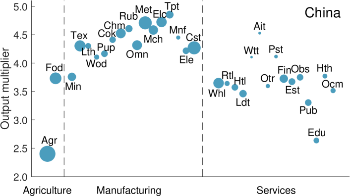
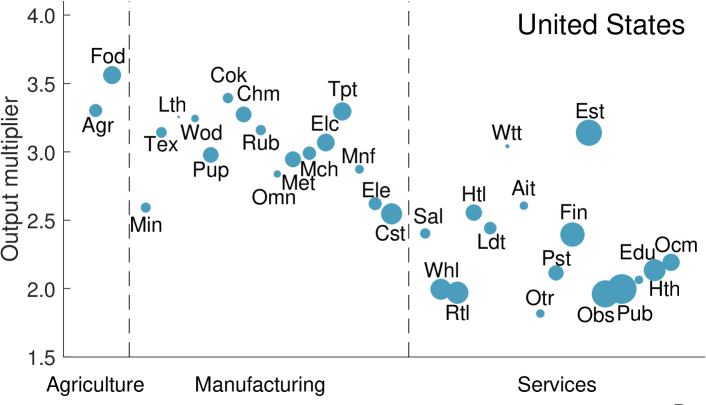
Figure 1: Output multipliers in Chinese and U.S. economies. Node size corresponds to gross output. Industry codes are given in Supplementary Information Table S1. All values are for 1995. Data source: World Input Output Database [20].

Output multipliers can also be expressed recursively as $\mathcal{L}_{i}=\sum_{j}\mathcal{L}_{j}a_{ji}+1$. One can think of this form in terms of an analogy with trophic structure, an organizing principle of ecology. In an ecosystem the trophic level of a species is informally its position on a food chain [30]; a simple ecosystem with grass, zebras, and lions would result in grass (the species at the bottom of the food chain) having a trophic level of one, zebras a trophic level of two, and lions three. Real ecosystems often have complex network structure, which include cycles and overlapping levels, and trophic levels are typically not integers but must be computed from a formula. One such formula [31] takes the recursive form above; letting $a^{\prime}_{ji}$ be the fraction of species $j$ in the diet of $i$, the trophic level of species $i$ is $\mathcal{L}^{\prime}_{i}=1+\sum_{j}\mathcal{L}^{\prime}_{j}a^{\prime}_{ji}$, i.e. 1 plus the average trophic level of the species it eats. Similarly the output multiplier of an industry is 1 plus the average output multiplier of the industries from which it buys inputs.

The recursive form makes clear that the output multiplier of an industry is influenced by two factors: the fraction of expenditures paid directly to households, and the output multipliers of the other inputs it buys. Higher labor expenditures make it more likely that a dollar spent will go directly to the household node, realizing the shortest possible path length of 1, and lowering the output multiplier. Similarly, dollars spent on goods from producers with high output multipliers will take more steps to reach the household node than dollars spent on goods with low output multipliers. In the special case where an industry $i$ buys no intermediate inputs, $i$ realizes the smallest possible production path length $\mathcal{L}_{i}=1$.

Examples of output multipliers for China and the United States are shown in Fig. 1. Each economy emphasizes different industries, but in both, manufacturing industries tend to have larger output multipliers than services (consistent with observations by Park and Chan [19]). In services, humans typically provide a larger share of inputs relative to intermediate goods. As a result, services may be expected to have shorter production chains. Output multipliers in China tend to be higher than in the U.S. because China’s household share of gross expenditures is lower. The differences in agriculture in the two countries is illustrative. In the U.S., agriculture is highly mechanized. Agricultural industries depend heavily on intermediate goods relative to capital and labor inputs. These industries have high output multipliers comparable to manufacturing. In China agriculture is more labor-intensive, giving it a comparatively low output multiplier.

Output multipliers have long been used to project the impacts of a change in final demand, such as a government stimulus (see e.g. [23]). Additional final demand for a good requires the industry making it to buy more inputs, increasing the production of the industries that supply its inputs, and setting off a ripple effect that raises the gross output of the economy. This amplification is greater when production chains are longer. This represents a different process from the one we study here. Nevertheless, the same network metric appears in both places in part because both processes involve a propagation of effects along production chains.

III Results

III.1 Network model of productivity improvement

Our baseline model uses basic results of productivity accounting and the assumption that the price of an industry’s good equals its marginal cost of production. Industry $i$ uses $\phi_{ij}$ of good $j$ and $\ell_{i}$ of labor per unit of output. Neglecting markups, the price $p_{i}$ of good $i$ equals its unit cost of production $p_{i}=\sum_{j}\phi_{ij}p_{j}+\ell_{i}w$ where $w$ is the wage rate. This equation determines prices, so as the matrix of input needs $\phi_{ij}(t)$ and $\ell_{i}(t)$ evolves, prices change accordingly. As shown in the Methods, the results can also be obtained in a general equilibrium framework (e.g. [32, 33, 13]). Here the key assumptions are that industries are price-takers who maximize profits at prevailing prices, subject to a production function with constant returns to scale, that consumers maximize utility subject to a budget constraint, and that prices instantaneously equilibrate supply and demand for all goods and labor. A key point of our baseline model is that we do not need to take a stand on the functional forms of utility and production functions. An extended presentation of this model can be found in the Supplementary Information.

Let $\widehat{\phi}_{ij}\equiv\dot{\phi}_{ij}/\phi_{ij}$ and $\widehat{\ell}_{i}\equiv\dot{\ell}_{i}/\ell_{i}$ denote the growth rates of $i$’s use of good $j$ and labor respectively. An industry’s improvement can be captured by its productivity growth rate $\gamma_{i}$ [16], which can be expressed as a cost-weighted average of the rates of change of its input uses: $\gamma_{i}=-(\sum_{j}\widehat{\phi}_{ij}a_{ji}+\widehat{\ell}_{i}\tilde{\ell}_{i})$. The minus sign reflects the fact that a reduction in input use corresponds to an increase in productivity. Let $r_{i}$ denote the log rate of change for the real (i.e. inflation-adjusted) price of industry $i$. To deflate prices, the wage rate in a country was computed as the ratio of the total labor income earned to total hours worked by industries in the country, and then the rate of change of the real price of industry $i$ in country $c$ was computed as $r_{i}=r_{i}^{\prime}-\rho_{c(i)}$, where $r_{i}^{\prime}$ is the log change in nominal price and $\rho_{c(i)}$ is the log change in the wage rate of the country $c$ to which industry $i$ belongs. Price changes can be expressed as

$$r_{i}=-\gamma_{i}+\sum_{j}r_{j}a_{ji}.$$ (2)

The first term captures industry $i$’s productivity improvement. The second is the rate of price change for the inputs $i$ purchases, and is the growth rate of a Divisia price index. Eq. (2) simply says that the change in the price of good $i$ equals the change in the cost of $i$’s inputs, minus an extra term that captures $i$’s technological improvement. Eq. (2) represents what is known as a dual approach to productivity analysis [16]. Typically, this approach is used to estimate productivity improvement, while here we are focused on modeling its effects.

The dynamics generated by this model are demonstrated in Fig. 2A. It depicts a circular economy that begins and ends with households. Households sell labor to industry $b$, which makes an intermediate good that is sold to industry $a$, which makes a final good sold to households. (For simplicity industry $a$ purchases no labor.) When the productivity of either industry rises it needs less input per unit of good produced, causing its price to fall due to a lowered cost of production. While industry $b$ only benefits from its own improvement, lower costs in this industry are passed on to $a$. The result is that good $a$’s price reduction is the sum of both improvement rates.

A
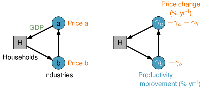
B

Figure 2: Productivity growth and prices. (A) A bare-bones production network. Arrows show direction of goods. Second diagram shows the price effects of productivity changes. Productivity growth rates $\gamma_{a}$ and $\gamma_{b}$ lead to rates of price change $r_{b}=-\gamma_{b}$ and $r_{a}=-\gamma_{a}-\gamma_{b}$. (B) The price change $r_{i}$ of an industry can be decomposed as $r_{i}=-\gamma_{i}+\sum_{j}r_{j}a_{ji}$, where $-\gamma_{i}$ is $i$’s direct contribution to its price reduction and $\sum_{j}r_{j}a_{ji}$ is the contribution from price changes passed to $i$ through input goods. Each distribution is a histogram of 30 bins. The direct component has larger variance, but the indirect component has lower mean, causing the larger share of price changes for a typical industry to be driven by its supply chain.

III.2 The importance of inherited improvement

Eq. (2) can also be taken as a decomposition of an industry’s price reduction. The term $-\gamma_{i}$ accounts for the direct benefits of $i$’s technology improvement, while the sum $\sum_{j}r_{j}a_{ji}$ accounts for the total effect of all other productivity gains in the network. This can be seen by writing Eq. (2) as $r_{i}=-\gamma_{i}-\sum_{k=1}^{\infty}\sum_{j}[(A^{T})^{k}\boldsymbol{\mathbf{\gamma}}]_{i}$ where $\boldsymbol{\mathbf{\gamma}}$ is the vector of productivity growth rates; see Supplementary Information. The second component accumulates productivity improvements in upstream industries over production paths of all lengths $k$. In this sense this term captures inherited improvement – accumulated productivity gains that are effectively passed to $i$ through reductions in input prices.

How much does inherited improvement contribute to price reduction in economies? Fig. 2B shows the distributions of the two components in the WIOD data. Industry price changes are highly correlated with both components, with a correlation of 0.92 to the direct component and 0.71 to the inherited component. (See the Supplementary Information for an extended discussion of these correlations.) The direct component has a broader distribution, and as a result explains more of the variation in price changes.

Nevertheless, the magnitudes of the two components (rather than the correlations) bear out a remarkable aspect of price evolution. On average, inherited price reductions contribute more to price reduction (mean value -1.65% yr^-1) than the direct components do (mean value -1.06% yr^-1). The average inherited cost reduction is about 1.6 times larger than the average direct component. Considering industries individually, the inherited component contributes the better part of an industry’s cost reduction in 64% of industries in the WIOD. As an example, from 1995 to 2009, the average price of electrical and optical equipment in China fell about 10% per year; a rapid rate of improvement. Out of this 10% though, 6.2% per year was inherited through the industry’s inputs.

It is not simply the case that inherited price reductions matter to fully account for price changes in an economy. Rather, most price reduction comes through lower prices in purchased inputs. This point also underscores a benefit of studying long-term price change in a production network setting, as price outcomes can be related to technology improvements in seemingly unrelated parts of the economy.

III.3 The output multiplier bias in price evolution

These observations highlight the ability of production networks to accumulate the effects of productivity improvements. How much this occurs for an individual industry depends on its position in the network. Solving Eq. (2) in vector form leads to $\boldsymbol{\mathbf{r}}=-H^{T}\boldsymbol{\mathbf{\gamma}}$, where $\boldsymbol{\mathbf{r}}$ is the vector of price changes, $\boldsymbol{\mathbf{\gamma}}$ is the vector of productivity growth rates, and $H\equiv(I-A)^{-1}$ is the Leontief inverse. This network relationship between prices and productivity growth rates follows immediately from dual approaches to productivity growth [16] and has been exploited in models (e.g. [33, 34]).

Let $\bar{\gamma}$ be the average productivity growth rate across industries, and write industry $i$’s productivity growth rate as the sum of the average and a deviation, $\gamma_{i}=\bar{\gamma}+\Delta\gamma_{i}$. The expected value of $r_{i}$ conditioned on the output multiplier is $E[r_{i}|\mathcal{L}_{i}]=-\bar{\gamma}\mathcal{L}_{i}-\sum_{j}E\left[\Delta\gamma_{j}H_{ji}\big{|}\mathcal{L}_{i}\right]$. Empirically the correlations of $\Delta\gamma_{j}$ with the matrix elements $H_{ji}$ are low (see Supplementary Information). Assuming $\Delta\gamma_{j}$ and $H_{ji}$ are uncorrelated, the second term is equal to zero, and we have

$$E[r_{i}|\mathcal{L}_{i}]=-\bar{\gamma}\mathcal{L}_{i}.$$ (3)

Eq. (3) says the expected price change in industries with output multiplier $\mathcal{L}_{i}$ is proportional to $\mathcal{L}_{i}$. This is because an industry benefits from both its own productivity improvement and the accumulation of upstream improvements. As a result, industries with longer production chains will be biased to experience faster price reduction. Eq. (3) indicates that the appropriate measure of production chain length for this mechanism is the output multiplier $\mathcal{L}_{i}$. This simple relationship, which is readily obtained from standard results, places emphasis on the output multipliers as network measures.

Figure 3: The output multiplier bias in price evolution. (A) Rates of price change for 1400 world industries versus industry output multipliers (orange dots). Industries with similar output multipliers are grouped into bins of $\sim$45 points each and the average price change is computed for each bin (brown dots). Vertical lines give error bars of two standard deviations around the bin mean. The black line is the theoretical prediction for the bin averages based on the relation $E[r_{i}|\mathcal{L}_{i}]=-\bar{\gamma}\mathcal{L}_{i}$ with $\bar{\gamma}$ equal to the mean of productivity growth rates over 1995 - 2009. (B-C) Price changes and output multipliers with a selection of services and manufacturing industries highlighted by black dots. (D) Variation in output multipliers predicts variation in price changes within industry categories. We remove dependence on industry category by standardizing observations by their cross-country averages and standard deviations, and comparing centered-and-normed price changes to centered-and-normed output multipliers. Black line is a regression fit.

We test this prediction by looking at price changes for the 1400 industries (40 countries $\times$ 35 industry categories) in the WIOD. We compute rates of real price change for the period 1995 - 2009 and compute output multipliers in 1995. Comparing these (Fig. 3A) shows the predicted, systematic deviation of the expected price change with the output multiplier; industries with larger output multipliers are biased to realize faster price reduction. Binning price changes by industry output multipliers and computing the average change in each bin gives an empirical estimate of the conditional expectation $E[r_{i}|\mathcal{L}_{i}]$. Regressing the bin averages on the output multipliers gives a slope $-1.6\%$ per year ($p\sim 10^{-8}$, $R^{2}=0.75$).

Alternatively, we can use Eq. (3) to make a prediction of $E[r_{i}|\mathcal{L}_{i}]$ without free parameters. We estimate $\bar{\gamma}=1.0\%$ per year using the productivity growth rates of industries over the period 1995 - 2009. Using this value in Eq. (3) yields the theory line in Fig. 3A. In either approach we fix the output multipliers at their values at the start of the period. Output multipliers help characterize network structure, and this probes the idea that this structure is sufficiently stable to approximate the accumulation of productivity improvement as a process on a static network. We see that output multipliers fixed at their initial values can predict subsequent changes in price. (We also find that using time-averages of the output multipliers yields very similar results, see Supplementary Information.)

The difference between the observed regression slope $-1.6\%$ per year and the predicted slope $-\bar{\gamma}=-1.0\%$ per year stems from a positive correlation between output multipliers $\mathcal{L}_{i}$ and productivity improvement rates $\gamma_{i}$, which have a Pearson correlation 0.11 ($p\sim 10^{-5}$). Productivity improvement rates tend to be greater for industries with higher output multipliers, increasing the magnitude of the slope in Fig. 3A. This correlation is outside the model of Eq. (2), but is not inconsistent with it – the model does not say what determines productivity. To see whether this correlation drives the relationship between price changes and output multipliers, we shuffle improvement rates across industries to remove the correlation with the output multipliers (Supplementary Information Fig. S2), finding that the output multipliers retain a highly significant correlation with price changes even with this effect removed.

Manufacturing industries are known to have higher output multipliers as well as faster price reduction (Fig. 3B-C), suggesting this could drive their correlation. But even within an industry category, a higher output multiplier predicts faster relative price reduction. Comparing centered-and-normed price changes with centered-and-normed output multipliers (i.e. applying fixed effects at the industry level) reveals a strong negative correlation of $-0.39$ ($p\sim 10^{-100}$) (Fig. 3D). This relationship also holds when we examine industries individually (Supplementary Information Table S3). We also divide industries into the broad groupings of manufacturing, services, and agriculture, and compare the predictive ability of these labels to that of output multipliers, finding the latter to be much better predictors of price change (Supplementary Information Table S4). While not central to our results, the correlation of price movements with network structure suggests there will also be structural correlations in the price movements of different industries with each other. We examine this possibility in the Supplementary Information, finding good agreement with the model here as well.

III.4 Increasing relevance of output multipliers with time

In Fig. 3A the price changes of industries have considerable dispersion around the expected value $E[r_{i}|\mathcal{L}_{i}]$. The characteristics of this dispersion are also predicted by Eq. (2). Let $r_{i}(t,t+T)$ be the average rate of change of price $i$ from $t$ to $t+T$. We study the behavior of $\sigma_{r_{i}(t,t+T)|\mathcal{L}_{i}}$, the standard deviation of $r_{i}(t,t+T)$ across industries with a given output multiplier. In the Supplementary Information, we compute the variance of Eq. (2), factoring out the dependence on the output multiplier, and approximate $\sigma_{r_{i}(t,t+T)|\mathcal{L}_{i}}$ as

$$\sigma_{r_{i}(t,t+T)|\mathcal{L}_{i}}\approx\frac{1}{\sqrt{T}}\Big{[}\sigma_{\gamma,\text{direct}}+\rho\sigma_{\gamma,\text{inherited}}(\mathcal{L}_{i}-1)$$

$$+\frac{1}{2}\frac{\sigma_{\gamma,\text{inherited}}^{2}}{\sigma_{\gamma,\text{direct}}}(\mathcal{L}_{i}-1)^{2}\Big{]}.$$ (4)

Here, $\sigma_{\gamma,\text{direct}}=(\text{Var}[\gamma_{i}|\mathcal{L}_{i}])^{1/2}$ is the standard deviation of the direct productivity benefit $\gamma_{i}$ across industries with output multiplier $\mathcal{L}_{i}$, $\sigma_{\gamma,\text{inherited}}(\mathcal{L}_{i}-1)$ is the standard deviation of the inherited productivity benefit $(\boldsymbol{\mathbf{\gamma}}^{T}A+\boldsymbol{\mathbf{\gamma}}^{T}A^{2}+\cdots)_{i}$ across industries with output multiplier $\mathcal{L}_{i}$, and $\rho$ is the Pearson correlation between direct and inherited benefits. (The coefficient $\frac{1}{2}\frac{\sigma_{\gamma,\text{inherited}}^{2}}{\sigma_{\gamma,\text{direct}}}$ is small compared with $\rho\sigma_{\gamma,\text{inherited}}$, and as a result the contribution of the quadratic term will be small.)

Eq. (4) makes two predictions (Fig. 4A). First, in any given time period, variation in price change is greater for industries with large output multipliers. Second, for any given output multiplier, this variation shrinks with time like $1/\sqrt{T}$. The second prediction means that dispersion in price changes around the expected value shrinks as the prediction horizon gets longer. As a result, the output multiplier of an industry becomes increasingly relevant for its price reduction over time.

A
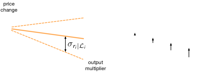
B
C

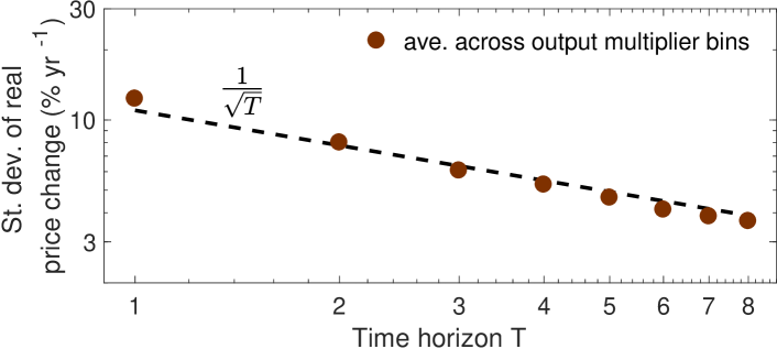
Figure 4: Cross-industry dispersion in price changes over different time horizons. (A) Predictions of Eq. (4) for cross-industry dispersion in rates of price change. (B) We examine average rates of price change $r_{i}(t,t+T)$ over horizons of $T$ = 1, 2, 4, and 8 years. Left panels show price changes for individual industries (orange dots). The average price change for industries in a given output multiplier bin (brown dots) gives an empirical estimate of the expected price reduction $E[r_{i}|\mathcal{L}_{i}]$. The black line is the theory prediction for this expected value. Right panels shows the standard deviation of price changes for industries with a given output multiplier (brown dots) and the theory prediction (black line). (C) Standard deviation of $r_{i}(t,t+T)$ for all industries. The dashed line is a guide to the eye and is proportional to $1/\sqrt{T}$.

We test these predictions with observations from the WIOD over the time horizons $T=$ 1, 2, 4, and 8 years (Fig. 4B-C). We again hold the output multipliers fixed at their values in the year 1995, exploiting the relatively slow rate of change of output multipliers over time. In addition to the dependence of $\sigma_{r_{i}(t,t+T)|\mathcal{L}_{i}}$ on $\mathcal{L}_{i}$ predicted by Eq. (4), we find an additional effect in which industries with larger output multipliers have larger variation in productivity improvement, leading to a dependence of $\sigma_{\gamma,\text{direct}}$ on $\mathcal{L}_{i}$. Similar to the correlation between productivity improvement and output multipliers, this correlation lies outside the theory here, though is not inconsistent with our findings. To take this correlation into account, for each time horizon we build a linear model of $\sigma_{\gamma,\text{direct}}$’s dependence on $\mathcal{L}_{i}$. This model by itself (without the additional terms in Eq. (4)) explains roughly 60% of the slope of $\sigma_{r_{i}(t,t+T)|\mathcal{L}_{i}}$, and thus by itself yields a poor fit to the data. We use this linear model within Eq. (4) to obtain the prediction for $\sigma_{r_{i}(t,t+T)|\mathcal{L}_{i}}$ for each time horizon and obtain a much better prediction, shown in Fig. 4B.

Over any given time horizon, price changes vary more among industries with large output multipliers (Fig. 4B). As time passes, this dispersion across industries shrinks at a rate in good agreement with the $1/\sqrt{T}$ prediction (Fig. 4C). (See also Supplementary Information and Fig. S3 for further discussion.) Note that the higher dispersion in price changes for industries with large output multipliers accounts for the triangular shape of price changes in Figs. 3-4. Over time this triangle narrows, with the expected value Eq. (3) becoming an increasingly good predictor, i.e. an industry’s price evolution becomes better predicted by a long-term behavior based on its output multiplier.

III.5 The average output multiplier and economic growth

We now consider the implications of the results above for economic growth. To the extent that an economy enjoys real price reductions by consuming more, falling prices will translate into greater output. The relationship of output multipliers with price reductions thus suggests a relationship with growth as well. Aggregating across price reductions in all industries, it can be shown (see e.g. [13] and Supplementary Information) that the real growth rate $g$ of a closed economy depends on productivity growth rates as $g=\boldsymbol{\mathbf{\theta}}^{T}H^{T}\boldsymbol{\mathbf{\gamma}}$.

A                                                                    B

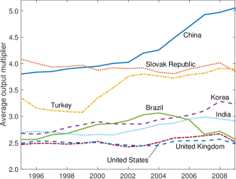
Figure 5: Productivity improvement and average output multipliers over time. (A) Average productivity improvement rate ($\tilde{\gamma}_{c}$) and (B) average output multiplier ($\bar{\mathcal{L}}_{c}$) for a selection of countries.

The rate of growth can be readily recast (see Supplementary Information) in terms of output multipliers as well, yielding

$$g=\tilde{\gamma}\bar{\mathcal{L}}.$$ (5)

Here $\tilde{\gamma}\equiv\sum_{i}\eta_{i}\gamma_{i}$ is the average rate of productivity improvement across a country’s industries with weights $\eta_{i}$ giving the share of industry $i$ in gross output (total revenue of all industries). The factor $\bar{\mathcal{L}}\equiv\sum_{i}\theta_{i}\mathcal{L}_{i}$ is the weighted average of industries’ output multipliers with $\theta_{i}$ giving the share of industry $i$ in final output (GDP). Eq. (5) predicts that the GDP growth of a country is proportional to the product of its average productivity improvement and its average output multiplier. It factors GDP growth into two parts, one that depends on productivity, and another that is purely a structural property of the economy’s production network. Thus, similar to Eq. (3), standard results can be manipulated to give a simple but novel expression that relates growth with production chain length and communicates readily with data.

The dynamics of $\tilde{\gamma}$ and $\bar{\mathcal{L}}$ differ in character (Fig. 5). The average improvement rate fluctuates considerably from year to year; the average output multiplier varies much more slowly. One way to quantify this difference is to compare the time variation in output growth, productivity improvement, and output multipliers. For each variable $X(t)$ we compute the coefficient of variation (CV) $\sigma_{X}/\mu_{X}$ where $\sigma_{X}$ is the time standard deviation (volatility) and $\mu_{X}$ is the time average from 1995 to 2009. Typical CVs (geometric mean across countries) are 1.4 for output growth, 2.3 for average productivity growth, and 0.041 for the average output multiplier. By this measure, average output multipliers have about $1.4/0.041\sim 34$ times less variation over time than growth rates do, and $2.3/0.041\approx 56$ times less variation than productivity improvement rates. (We similarly find that industry-level output multipliers have $2.47/0.057\approx 43$ times less variation than price changes and $3.8/0.057\approx 66$ times less variation than productivity improvement.) As with individual industries, this relative persistence at the aggregate level makes intuitive sense given that underlying production relationships take time to change. A difference at the aggregate level is that $\bar{\mathcal{L}}$ may change because of shifts in an economy’s final output mix, even if its industry-level output multipliers $\mathcal{L}_{i}$ were to remain the same, a point we revisit in the Discussion.

The persistence of $\bar{\mathcal{L}}$ in Eq. (5) suggests that a country’s average output multiplier should not only correlate with its current growth rate but also with its growth rate for some time into the future. In the WIOD data (Fig. 6A) the growth rates of real GDP per hour over 1995 - 2009 have a Pearson correlation $\rho=0.53$ ($p=4\times 10^{-4}$) with countries’ average output multipliers in the initial year 1995. For longer production chains to result in faster growth, the average rate of productivity improvement of an economy must not decrease as the average output multiplier gets larger. In fact we observe the opposite tendency; the positive correlation noted earlier between productivity growth and output multipliers at the industry level now appears as a positive correlation at the aggregate level ($\rho=0.45$) between $\tilde{\gamma}$ and $\bar{\mathcal{L}}$. We do not attempt to explain the correlation here, though it is plausible that factors such as investment would increase both the length of production chains and the rate of technological improvement at the same time. This correlation means that the regression relation between growth and output multipliers in Fig. 6A reflects two effects: the theoretical prediction that, all else equal, countries with larger average output multipliers should grow faster, and the empirical observation that countries with larger average output multipliers tend to have higher average productivity growth rates.

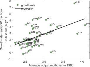
A                                                                        B
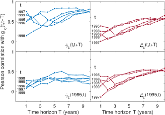
C

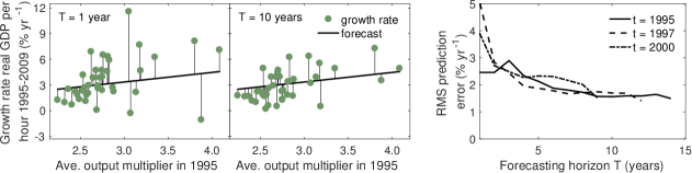
Figure 6: Country growth and the average output multiplier. (A) Growth rates of real GDP per hour over 1995 - 2009 for 40 WIOD countries versus $\bar{\mathcal{L}}$ in 1995. Solid line is an OLS regression fit. Country codes are given in Supplementary Information Table S2. (B) Correlation of growth with average productivity growth rate and average output multiplier as time passes. For each country $c$ we compute the time-average growth rate $g_{c}$(t,t+T) from year t to year t+T. Top panels show the correlation of $g_{c}$(t,t+T) (across countries) with time-average productivity improvement ($\tilde{\gamma}_{c}$(t,t+T)) and time-average output multiplier ($\bar{\mathcal{L}}_{c}$(t,t+T)) over the same period (t,t+T). Bottom panels show the correlation of growth in (t,t+T) with productivity improvement and average output multipliers from the prior period (1995,t). (C) Simple forecast of country growth rates from multiplying countries’ average output multipliers in a starting year t by the mean improvement rate across all countries and years of our data prior to t. Left panels show forecasted and actual growth for starting year t = 1995. Right panel shows root mean square prediction error over a range of horizons with starting years 1995, 1997, and 2000.

While $\tilde{\gamma}$ and $\bar{\mathcal{L}}$ enter Eq. (5) symmetrically, these variables have fundamentally different characters. The average productivity growth rate is a rate-of-change, measured between two end times, while the average output multiplier is a state variable measured at a point in time. The former is noisy and the latter persistent. As theory predicts, both factors have high correlations with growth that rise with the length of the period one examines (Fig. 6B, top panels), but the reasons for this rise differ for each factor. For $\tilde{\gamma}$, examining a longer period means integrating over more of a country’s history of productivity gains; whether an economy realized years of rapid or sluggish improvement significantly influences whether these were also years of rapid growth. For $\bar{\mathcal{L}}$ however, examining a longer time period does not improve its correlation with growth by averaging over its own history, but by giving time for the fluctuations in the productivity factor to average out. Unlike the productivity growth rate the correlation of $\bar{\mathcal{L}}$ with growth is not sensitive to using values from the period in which the growth is observed (Fig. 6B, bottom panels).

These observations and theory suggest that the output multiplier should be able to forecast growth. We examine this possibility with an extremely simple forecasting model. From the perspective of an observer in year $t$, we conduct a forecast for the next $T$ years, in which we multiply the average output multiplier $\bar{\mathcal{L}}_{c}$ of every country in year $t$ by a representative guess of $\tilde{\gamma}$ for the future. Here we use the average of $\tilde{\gamma}$ across all countries in the years of our data leading up to $t$. By doing this we are also removing all cross-country variation in productivity growth to focus solely on the predictive power of the output multiplier. Remarkably, and despite the clear simplicity of this forecasting model, prediction error falls as the forecasting period grows (Fig. 6C). As noted already this occurs because output multipliers are persistent quantities and longer horizons provide more averaging over productivity growth fluctuations.

Strictly, this analysis does not identify the output multiplier as a causal factor; rather it demonstrates that the structure of the production network helps forecast growth. Yet there are at least four reasons to interpret it causally: (i) These forecasts are consistent with a clear causal mechanism generically implied by standard production network models; (ii) they emerge directly from the aggregation of the price effects documented earlier; (iii) they come with no free parameters; and (iv) are consistent with not just the sign of the effect, but its predicted functional form.

Finally, we note that the structural significance of $\bar{\mathcal{L}}$ is enhanced by a remarkable theorem by Fally (2012) [28] and Finn (1976) [35]. Data on production networks vary in level of aggregation from a few industries to hundreds, raising the concern that the average output multiplier varies with the granularity of the data. But it can be shown that the average output multiplier of a closed economy is independent of aggregation and equal to the ratio $\bar{\mathcal{L}}=\mathcal{O}/Y$ where $\mathcal{O}$ is gross output and ${Y}$ is net output (GDP) [28]. In the Supplementary Information we discuss this point further, and also examine it in the practical context of an open economy.

This result is important also because it implies that economies with very different production networks, but the same ratio $\mathcal{O}/Y$, would experience the same amplification to growth. Three comments are in order here. First, we note that the independence of the rate of growth from network structure is an approximation, reflecting the first order nature of our growth result. When we consider second order effects on growth (36), the details of the network can become relevant through the effects that relative price changes have on consumption shares and input shares. (Though we find evidence that such effects are modest for the time scales we study here, see Supplementary Information). Second, the fact that there exist macro-level sufficient statistics to characterize growth amplification does not imply there is no value in understanding its emergence as a network outcome. In particular, it takes a well-specified model to understand whether and how these sufficient statistics provide good approximations or whether they fail under certain circumstances. Third, in addition, our production network environment delivers testable micro-level predictions on sectoral relative price evolution that are important in themselves. The fact that these micro-predictions are in good agreement with data suggests that production networks can provide a causal mechanism (as opposed to reduced form, sufficient statistics) for differences in growth across countries.

IV Discussion

Economics has emphasized the outsized role of productivity in explaining cross-country differences in growth, and our theory features this. But production network models predict that variation in the output multiplier matters as well. These models generate a variety of predictions for how the output multiplier should shape price evolution and growth, with which observations from data are in good agreement. Recent studies [28, 26] have emphasized that the output multiplier can be understood as the average length of an industry’s production chains. This leads to an intuitive mechanism driving our results: An industry benefits from its own productivity gains, and that of upstream suppliers, and so the effects of productivity improvement accumulate along production chains. As a result, two countries realizing the same average micro-level productivity improvement can, if their production networks differ in depth, experience different aggregate growth rates.

At a micro level, the results suggest one reason why some technologies improve more rapidly than others, especially a version of this question that arises in Baumol’s classic observation. As confirmed many times since, in the 1960s Baumol observed that some industries, particularly manufacturers, realize productivity gains more rapidly than others [21, 36], and that over long periods such sustained differences will significantly impact prices. The relative prices of quickly-improving industries will naturally fall, but those of slower-improving industries (including many services) will increase, even if these industries are realizing some improvement [21]. This effect has often been cited as a cause of long-term price increases in health care [37] and education [38]. The results here point to a reason why manufacturing would be able to sustain faster improvement for long periods. Observations of output multipliers [19] reinforce the intuitive idea that manufacturing industries tend to have longer production chains than services. Manufacturing industries are advantaged by their network positions to benefit more greatly from productivity gains across the network. The results here suggest a nuanced way to help distinguish fast and slow segments of an economy, in that part of what helps define the fast-improving segment is the set of industries with large output multipliers rather than manufacturers per se. In particular, the fact seen earlier that output multipliers retain their predictive power within broad industries suggests that our analysis provides a more operational way to distinguish fast- and slow-improving industries.

At the aggregate level, the results suggest a new perspective on the long process of structural change [22], emphasizing changes to the length of an economy’s production chains. One expects an undeveloped economy to have short chains of production. As manufacturing becomes more prominent, the average output multiplier increases. Finally, as service industries become more prominent, the average output multiplier decreases. The predictions here suggest that, all else equal, an economy will accelerate its growth during the manufacturing stage and relax to slower growth when it becomes more developed. In Fig. 6a, developed economies have low average output multipliers and low growth rates while economies that are developing a strong manufacturing sector, such as China or Slovakia, tend to have high average output multipliers and high growth. The WIOD [20] does not contain data for undeveloped countries and we cannot confirm that their average output multipliers are low, though it would be surprising if it were otherwise.

To get a feel for the amplification to growth associated with production chains we consider some rough figures. In Fig. 5, China’s average output multiplier increases from 3.8 to 5 from 1995 to 2009. Had it not done this, Eq. (5) implies that its growth rate at the end of the period would have been reduced by a factor $3.8/5\approx 0.76$. More drastically, suppose China had the output multiplier of the United States of about 2.5, and as a rough figure take China’s output multiplier over the period to be its midpoint around 4.4. If China otherwise had the same average productivity improvement, its growth would have been smaller by a factor $2.5/4.4\approx 0.57$, i.e. close to half of its growth during the period would have been lost.

The results suggest that differences in the average output multiplier have been an important factor in the large income differences that exist across countries. These income differences originated in changes that economies underwent during industrialization [39, 40], when we would expect production chains to have started becoming more developed. The potential for the average output multiplier to help explain disparate income levels has not gone unnoticed. Jones [5, 41] notes that accounting for intermediate goods in models of aggregate production can generate large multiplier effects, with values that help explain observed differences in income.

Our results suggest that policy-makers may want to design network-aware industrial policies, targeting particular nodes in the production network. Our results per se do not rationalize policy intervention, but could be combined with a theory of distortions in the network such as sector-specific credit market distortions, product or input market imperfections, or, more generally, wedges. We conjecture that in certain settings policy-makers would target nodes relying on longer chains of production, though network-targeting prescriptions may depend in detail on the nature of the distortions (e.g. size, functional form, the loss function to be minimized, and so on.) Arguments for such network targeting policies are developed further in other works (e.g. [42, 43, 44]).

Our results show that the structure of a production network, taken as given, can serve as a proximate cause of growth differences across countries. A natural follow-up question is how the production network evolves and how two-way causal relations between growth and production networks function. For example, growth over long periods usually comes with shifts in the consumption basket (43), which will slowly change the output multiplier of an economy as noted earlier. Furthermore, one may also expect rising real wages to drive innovations that reduce labor needs relative to intermediate goods [45]. Such changes will tend to lengthen production chains over time. Finally, international trade, by inducing changes in both production and final demand patterns, offers another potential source of dynamics in the production network. For example, in our simple framework, when two countries open to trade their average output multipliers will become more similar; see Supplementary Information. This suggests that trade openness induces cross-country convergence in growth rates through changes in the production network, a result echoing previous arguments in the economic growth literature [46]. In all, the results here call for further investigations that include endogenizing the slow evolution of production networks over the growth process, and further exploring the role of production networks in long-term growth.

V Materials and methods

V.1 Data

We use data from the World Input-Output Database (WIOD) [20], which contains worldwide input-output tables across time for 35 industries in 40 countries, together accounting for around 88% of world GDP. Our analysis covers the period 1995 - 2009. We excluded 2010 and 2011 from analysis because a large number of countries lacked data on labor compensation required to compute the output multipliers (see below). The data also include production price indices from which we computed rates of price change. Since the period 2007-2009 may be regarded as exceptional because of the Great Recession we also checked the effect of excluding these years, finding very similar results (Supplementary Materials).

V.2 Output multipliers

We treated the world as one large economy and examined the $1400\times 1400$ matrix $A$ of input coefficients corresponding to all industries in all countries. We took the Leontief inverse and computed the $1400$-dimensional vector $\boldsymbol{\mathbf{\mathcal{L}}}=(I-A^{T})^{-1}\boldsymbol{\mathbf{1}}$ whose elements give the output multiplier of each industry in each country. Industries and their output multipliers are listed in Supplementary Information Table S1.

We considered two ways of computing industry output multipliers based on two interpretations of the labor coefficient $\tilde{\boldsymbol{\mathbf{\ell}}}$. In the first case we interpret $\tilde{\boldsymbol{\mathbf{\ell}}}$ to account for all factor payments to households (value added, row code r64). In the second case we interpret $\tilde{\boldsymbol{\mathbf{\ell}}}$ to account for households’ labor income only (using the labour compensation field and WIOD exchange rates to convert to U.S. dollars). In each case the total expenditures $M_{j}$ of each industry $j$ were computed, either including or excluding the non-labor factor payments of $j$, and then its input coefficients computed as $a_{ij}=M_{ij}/M_{j}$ where $M_{ij}$ is industry $j$’s payments to industry $i$. The results were qualitatively similar either way, and the results reported here use the latter calculation. The main difference between the approaches is that the output multipliers are smaller when including all payments to households. This increases the share of payments made to the household sector, thus shortening average path lengths.

WIOD did not contain data for labor and capital income separately for the Rest Of the World (ROW) region. We compared the results of excluding ROW altogether with including it using an assumed fraction of value added to represent labor income. We found very similar results either way. Results shown are based on including ROW with an assumed labor fraction 0.5, similar to the global average (0.57 in 2009) computed across the WIOD countries.

The average output multiplier of each country is the weighted sum of the output multipliers of its industries. The weight of industry $i$ in country $c$ was given by the share of $i$ in $c$’s contribution to world final demand, i.e. $Y_{i}/\sum_{j\in c}Y_{j}$ where $Y_{i}$ is the world final demand for good $i$. The final demand $Y_{i}$ accounts for consumption and investment payments by all countries (i.e. column codes c37-c42, summed over countries) and excludes net exports, since in WIOD the latter are accounted for within the input-output table. Countries and their average output multipliers are listed in Supplementary Information Table S2.

V.3 Price changes and productivity growth rates

The change $r_{i}^{\prime}$ in the nominal price of industry $i$ was computed as the annual log changes in the industry’s gross output price index. The wage rate in a country was computed as the ratio of the total labor income earned to total hours worked by industries in the country, and the log change in the wage rate was computed to give $\rho_{c}$. The rate of change of the real price of industry $i$ in country $c$ was then computed as $r_{i}=r_{i}^{\prime}-\rho_{c(i)}$ where $c(i)$ is the country $c$ to which industry $i$ belongs.

Productivity improvements rates were estimated as $\boldsymbol{\mathbf{\hat{\gamma}}}=(A^{T}-I)\boldsymbol{\mathbf{r}}$. This method represents a dual approach to estimating productivity changes [16, 47], in which the average growth rate of an industry’s input prices is computed and the growth of its output price is subtracted off, with the difference ascribed to improvements by the industry. An industry $j$’s productivity improvement $\gamma_{j}$ is its direct component of cost reduction, while the indirect component is the cost reduction $\sum_{i}r_{i}a_{ij}$ it inherits through inputs. At the country level, the average productivity improvement rate $\tilde{\gamma}_{c}$ for country $c$ was estimated as $\hat{\tilde{\gamma}}_{c}=\sum_{i\in c}\eta_{i}\,\hat{\gamma}_{i}$, where $\eta_{i}$ is the share of industry $i$ in the gross output of country $c$ to which it belongs.

V.4 Growth rates

We computed country growth rates with data from the World Bank’s World Development Indicators [48]. GDP in current local currency was deflated using each country’s GDP deflator, then divided by hours worked by persons engaged across all industries using WIOD socioeconomic data. Annual growth rates were then computed as the log change between consecutive years. Data for Taiwan was unavailable from the World Development Indicators, and we instead used data from the Penn World Tables [49].

V.5 General equilibrium framework for Eqs. (3)-(5)

In our baseline model (presented in the Supplementary Information) accounting identities and input-output relationships are used as the starting point to derive Eq. (2), from which the predictions Eqs. (3) - (5) follow. This approach has the advantage of enabling powerful results within the simple framework of accounting relationships. However, Eq. (2) can also be readily obtained in a general equilibrium framework following e.g. Long and Plosser [32], Acemoglu et al. [13], Baqaee and Farhi [50]. This reinforces the fact that, for the central predictions of this paper, we do not need to take a stand on the functional form of utility and production functions. In this section our objective is to show how Eq. (2) can be obtained in a general equilibrium framework. From either framework, the predictions Eqs. (3) - (5) follow as shown in the Supplementary Information.

Let $\boldsymbol{\mathbf{X}}_{i}\equiv(X_{i1},\,\ldots,\,X_{iN},L_{i})$ denote the vector of input rates to industry $i$, and assume non-joint production. Producer $i$ has a production function $f_{i}(\boldsymbol{\mathbf{X}}_{i},t)$ that at any given time $t$ characterizes the best available (i.e. Pareto efficient) production methods.

Industries are assumed to be price-takers who maximize profits at prevailing prices. The demand for inputs by industry $i$ is

$$\boldsymbol{\mathbf{X}}_{i}(\boldsymbol{\mathbf{p}},t)\equiv\arg\max_{\boldsymbol{\mathbf{X}}_{i}}\;f_{i}(\boldsymbol{\mathbf{X}}_{i},t)p_{i}-\boldsymbol{\mathbf{X}}_{i}\cdot\boldsymbol{\mathbf{p}},$$ (6)

where $\boldsymbol{\mathbf{p}}=(p_{1},\ldots,p_{N},w)$ is the vector of prices. Households are assumed to maximize a utility function $U(\boldsymbol{\mathbf{C}})$ subject to the budget constraint $\boldsymbol{\mathbf{C}}\cdot\boldsymbol{\mathbf{p}}=Lw$, yielding the vector $\boldsymbol{\mathbf{C}}(\boldsymbol{\mathbf{p}},L)$ of households’ demand functions for each good.

At equilibrium, prices $\boldsymbol{\mathbf{p}}$ are such that all markets (goods and labor) clear:

$$\sum_{j}X_{ji}(\boldsymbol{\mathbf{p}},t)+C_{i}(\boldsymbol{\mathbf{p}},L) =f_{i}\big{(}\boldsymbol{\mathbf{X}}_{i}(\boldsymbol{\mathbf{p}},t),t\big{)}\quad\text{for all $i$}$$ (7)

$$\sum_{i}L_{i}(\boldsymbol{\mathbf{p}},t) =L.$$ (8)

Assume that industries always have production possibilities $f_{i}(\boldsymbol{\mathbf{X}}_{i},t)$ characterized by constant returns to scale. Under these conditions, industries earn no economic profit at equilibrium, and activities earning deficits are not operated. Without loss of generality, let $i$ index only industries with positive output levels. Since these producers earn zero profit at equilibrium, revenues and expenditures satisfy the balance relation

$$\sum_{j}X_{ji}p_{i}+C_{i}p_{i}=\sum_{j}X_{ij}p_{j}+L_{i}w\qquad\text{for all $i$}.$$ (9)

This is the accounting identity for industry $i$ in an input-output table, with the balancing item of valued added corresponding to the sum over primary input payments. The model above thus gives these observed payments an interpretation as an outcome of an economy in general equilibrium.

Technology improvement, as captured by productivity growth, is represented by the advance of the Pareto frontier of the best available production methods. This is given by the partial derivative of the production function $f_{i}(\boldsymbol{\mathbf{X}}_{i},t)$ with respect to time while holding inputs to $i$ fixed. For convenience we use the hat notation to denote the growth rate of a variable, e.g. $\widehat{X}_{i}=\dot{X}_{i}/X_{i}$. Taking the time-derivative of $\ln f_{i}$ and solving for the partial derivative with respect to time leads to $i$’s productivity growth rate,

$$\gamma_{i}\equiv\frac{\partial\ln f_{i}}{\partial t}=\widehat{X}_{i}-\sum_{j}\epsilon_{ij}\widehat{X}_{ij}-\epsilon_{iL}\widehat{L}_{i},$$ (10)

where $\epsilon_{ij}\equiv\partial\ln f_{i}/\partial\ln X_{ij}$ is $i$’s output elasticity with respect to input $j$.

When producers are profit-maximizers under perfect competition, and production functions have constant returns to scale, the share of expenditures $a_{ji}$ that industry $i$ spends on input $j$ equals the output elasticity $\epsilon_{ij}$, a condition known as allocative efficiency. This follows from the first-order conditions of Eq. (6), which lead to $p_{j}/p_{i}=\partial f_{i}/\partial X_{ij}$ for all inputs $j$. Multiplying by $X_{ij}/X_{i}$ gives

$$a_{ji}=\frac{X_{ij}p_{j}}{X_{i}p_{i}}=\frac{\partial\ln f_{i}}{\partial\ln X_{ij}}=\epsilon_{ij}.$$ (11)

Using this, Eq. (10) becomes

$$\gamma_{i}=\widehat{X}_{i}-\sum_{j}\widehat{X}_{ij}a_{ji}-\widehat{L}_{i}\ell_{i}.$$ (12)

Eq. (12) is the residual expression of productivity improvement, in which the growth in output not explained by the average growth in input usage is attributed to productivity growth.

To see how productivity growth affects prices, we take the time-derivative of the logarithm of Eq. (9). Noting that $\sum_{j}X_{ji}+C_{i}$ is $i$’s total production $X_{i}$, this leads to

$$\widehat{X}_{i}+\widehat{p}_{i}=\sum_{j}\left(\widehat{X}_{ij}+\widehat{p}_{j}\right)a_{ji}+(\widehat{L}_{i}+\widehat{w})\ell_{i}.$$ (13)

Using the fact that $\ell_{i}=1-\sum_{j}a_{ji}$, after rearrangement we have

$$\widehat{p}_{i}-\widehat{w}=-\left(\widehat{X}_{i}-\sum_{j}\widehat{X}_{ij}a_{ji}-\widehat{L}_{i}\ell_{i}\right)+\sum_{j}(\widehat{p}_{j}-\widehat{w})a_{ji}.$$ (14)

The term in parentheses is the productivity growth rate of $i$, Eq. (12). Defining the real price changes $r_{i}\equiv\widehat{p}_{i}-\widehat{w}$, we then have

$$r_{i}=-\gamma_{i}+\sum_{j}r_{j}a_{ji}$$ (15)

which is Eq. (2). From here, the predictions Eqs. (3) - (5) follow as described in the Supplementary Information.

References

- [1] Leontief, W. W. Quantitative input and output relations in the economic systems of the United States. Rev. Econ. Statistics 18, 105–125 (1936).
- [2] Leontief, W. Input-Output Economics (Oxford University Press, 1986).
- [3] Xu, M., Allenby, B. R. & Crittenden, J. C. Interconnectedness and resilience of the US economy. Adv. Complex Syst. 14, 649–672 (2011).
- [4] Atalay, E., Hortaçsu, A., Roberts, J. & Syverson, C. Network structure of production. Proc. Natl. Acad. Sci. U.S.A. 108, 5199–5202 (2011).
- [5] Jones, C. I. Intermediate goods and weak links in the theory of economic development. Am. Econ. J. - Macrecon. 3, 1–28 (2011).
- [6] McNerney, J., Fath, B. D. & Silverberg, G. Network structure of inter-industry flows. Physica A 392, 6427–6441 (2013).
- [7] Carvalho, V. M. Aggregate Fluctuations and the Network Structure of Intersectoral Trade. Ph.D. thesis, University of Chicago (2008).
- [8] Antràs, P., Chor, D., Fally, T. & Hillberry, R. Measuring the upstreamness of production and trade flows. Am. Econ. Rev. 102, 412–416 (2012).
- [9] Blöchl, F., Theis, F. J., Vega-Redondo, F. & Fisher, E. O. Vertex centralities in input-output networks reveal the structure of modern economies. Phys. Rev. E 83, 046127 (2011).
- [10] Horvath, M. Sectoral shocks and aggregate fluctuations. J. Monetary Econ. 45, 69–106 (2000).
- [11] Foerster, A. T., Sarte, P.-D. G. & Watson, M. W. Sectoral versus aggregate shocks: A structural factor analysis of industrial production. J. Polit. Econ. 119, 1–38 (2011).
- [12] Gabaix, X. The granular origins of aggregate fluctuations. Econometrica 79, 733–772 (2011).
- [13] Acemoglu, D., Carvalho, V. M., Ozdaglar, A. & TahBaz-Salehi, A. The network origins of aggregate fluctuations. Econometrica 80, 1977–2016 (2012).
- [14] Contreras, M. G. A. & Fagiolo, G. Propagation of economic shocks in input-output networks: A cross country analysis. Phys. Rev. E 90, 062812 (2014).
- [15] Solow, R. M. A contribution to the theory of economic growth. Q. J. Econ. 70, 65–94 (1956).
- [16] Jorgenson, D., Gollop, F. M. & Fraumeni, B. P, vol. 169 (Elsevier, 1987).
- [17] Domar, E. D. On the measurement of technological change. Econ. J. 71, 709–729 (1961).
- [18] Hulten, C. R. Growth accounting with intermediate inputs. Rev. Econ. Stud. 45, 511–518 (1978).
- [19] Park, S.-H. & Chan, K. S. A cross-country input-output analysis of intersectoral relationships between manufacturing and services and their employment implications. World Dev. 17, 199–212 (1989).
- [20] Timmer, M. P., Dietzenbacher, E., Los, B., Stehrer, R. & De Vries, G. J. An illustrated user guide to the world input–output database: the case of global automotive production. Rev. Int. Econ. 23, 575–605 (2015).
- [21] Baumol, W. J. Macroeconomics of unbalanced growth: The anatomy of urban crisis. Am. Econ. Rev. 57, 415–426 (1967).
- [22] Kuznets, S. Quantitative aspects of the economic growth of nations: Ii. industrial distribution of national product and labor force. Econ. Dev. Cult. Change 5, 1–111 (1957).
- [23] Miller, R. E. & Blair, P. D. Input-Output Analysis: Foundations and Extensions (Cambridge University Press, 2009).
- [24] Kemeny, J. G. & Snell, J. L. Finite Markov Chains (Van Nostrand, 1960).
- [25] Hirschmann, A. The Strategy of Economic Development (Yale University Press, 1958).
- [26] Miller, R. E. & Temurshoev, U. Output upstreamness and input downstreamness of industries/countries in world production. Int. Regional Sci. Rev. 40, 443–475 (2017).
- [27] Katz, L. A new status index derived from sociometric analysis. Psychometrika 18, 39–43 (1953).
- [28] Fally, T. Production staging: measurement and facts. Ph.D. thesis, University of Colorado Boulder (2012).
- [29] Leontief, W. & Brody, A. Money-flow computations. Econ. Syst. Res. 5, 225–233 (1993).
- [30] Post, D. M. The long and short of food-chain length. Trends Ecol. Evol. 17, 269 – 277 (2002).
- [31] Levine, S. Several measures of trophic structure applicable to complex food webs. J. Theor. Biol. 83, 195–207 (1980).
- [32] Long, J. & Plosser, C. Real business cycles. J. Polit. Econ. 91, 39–69 (1983).
- [33] Balke, N. S. & Wynne, M. A. An equilibrium analysis of relative price changes and aggregate inflation. J. Monetary Econ. 45, 269–292 (2000).
- [34] Carvalho, V. M. & Tahbaz-Salehi, A. Production networks: A primer. Annual Review of Economics 11, 635–663 (2019).
- [35] Finn, J. T. Measures of ecosystem structure and function derived from analysis of flows. J. Theor. Biol. 56, 363–380 (1976).
- [36] Nordhaus, W. D. Baumol’s diseases: a macroeconomic perspective. BE J. Macroecon. 8 (2008).
- [37] Bates, L. J. & Santerre, R. E. Does the us health care sector suffer from baumol’s cost disease? evidence from the 50 states. J. Health Econ. 32, 386–391 (2013).
- [38] Baumol, W. J. Children of performing arts, the economic dilemma: The climbing costs of health care and education. J. Cult. Econ. 20, 183–206 (1996).
- [39] Bairoch, P. International industrialization levels from 1750 to 1980. Journal of European Economic History 11, 269 (1982).
- [40] Galor, O. Unified growth theory (Princeton University Press, 2011).
- [41] Jones, C. Advances in Economics and Econometrics, chap. Misallocation, Economic Growth, and Input-Output Economics (Westview Press, 2013).
- [42] Liu, E. Industrial policies in production networks. The Quarterly Journal of Economics 134, 1883–1948 (2019).
- [43] Bigio, S. & La’o, J. Distortions in production networks. The Quarterly Journal of Economics 135, 2187–2253 (2020).
- [44] Baqaee, D. R. & Farhi, E. Productivity and misallocation in general equilibrium. The Quarterly Journal of Economics 135, 105–163 (2020).
- [45] Kennedy, C. Induced bias in innovation and the theory of distribution. The Economic Journal 74, 541–547 (1964).
- [46] Ben-David, D. Equalizing exchange: Trade liberalization and income convergence. The Quarterly Journal of Economics 108, 653–679 (1993).
- [47] Organization for Economic Cooperation and Development. Measuring Productivity - OECD Manual: Measurement of Aggregate and Industry-level Productivity Growth. Tech. Rep. (2001).
- [48] The World Bank. World Bank Development Indicators (2018). URL http://data.worldbank.org/.
- [49] Feenstra, R. C., Inklaar, R. & Timmer, M. P. The next generation of the Penn World Table. Am. Econ. Rev. 105, 3150–3182 (2015).
- [50] Baqaee, D. R. & Farhi, E. The macroeconomic impact of microeconomic shocks: Beyond Hulten’s Theorem. Econometrica 87, 1155–1203 (2019).