Temporal stability analysis of jets of lobed geometry

Abstract

A 2D temporal incompressible stability analysis is carried out for lobed jets. The jet base flow is assumed to be parallel and of a vortex-sheet type. The eigenfunctions of this simplified stability problem are expanded using the eigenfunctions of a round jet. The original problem is then formulated as an innovative matrix eigenvalue problem, which can be solved in a very robust and efficient manner. The results show that the lobed geometry changes both the convection velocity and temporal growth rate of the instability waves. However, different modes are affected differently. In particular, mode $0$ is not sensitive to the geometry changes, while modes of higher-orders can be changed significantly. The changes become more pronounced as the number of lobes $N$ and the penetration ratio $\epsilon$ increase. Moreover, the lobed geometry can cause a previously degenerate eigenvalue ($\lambda_{n}=\lambda_{-n}$) to become non-degenerate ($\lambda_{n}\neq\lambda_{-n}$) and lead to opposite changes to the stability characteristics of the corresponding symmetric ($n$) and antisymmetric ($-n$) modes. It is also shown that each eigen-mode changes its shape in response to the lobes of the vortex sheet, and the degeneracy of an eigenvalue occurs when the vortex sheet has more symmetric planes than the corresponding mode shape (including both symmetric and antisymmetric planes). The new approach developed in this paper can be used to study the stability characteristics of jets of other arbitrary geometries in a robust and efficient manner.

1 Introduction

Aircraft noise reduction is an urgent issue nowadays. Among the many noise sources of an aircraft, jet noise is still a significant contributor. This is especially true when an aircraft is taking off. While the exact role played by jet instabilities in noise generation is still open to some debate for subsonic jets, recent studies (Cavalieri et al., 2014; Piantanida et al., 2016; Lyu & Dowling, 2016; Lyu et al., 2017) show that installed jet noise is dominated by the scattering of jet instability waves by the trailing edge of aircraft wings or flaps. To suppress or reduce installed jet noise, one can examine the possibility of controlling these instability waves. Since instability waves are closely related to jet mean flows, one such an approach is to modify jet mean flows to become less axisymmetric. The feasibility of this approach, however, hinges on the hope that the instability waves can be somehow suppressed by using a less axisymmetric jet mean flow. This raises the question of examining the stability characteristics of jets of general non-axisymmetric geometries.

Though jet instability is among the most heavily studied areas in fluid mechanics (Morris, 2010), the research on the characteristics of the instability waves of non-axisymmetric jets is rather limited. Some of the early attempts include those on elliptic and rectangular jets. These include some analytical (Crighton, 1973), numerical (Morris, 1988; Tam & Thies, 1993; Baty & Morris, 1995) and some relevant experimental studies focusing on the turbulence, mixing and acoustics of non-axisymmetric jets (Tam & Zaman, 2000; Li et al., 2002; Zaman et al., 2003; Miao et al., 2015; Li et al., 2001, 2002; Hu et al., 2002). The analytical work of Crighton (1973) showed that separable solutions can be obtained for elliptic jets. The instability waves aligned with the major and minor axes exhibit different behaviours. Not surprisingly, the instability waves of rectangular jets share similar characteristics (Tam & Thies, 1993). Analytical works normally assumed the mean flow to be of a vortex sheet type to allow mathematical derivations to proceed. For more realistic jet mean flows, numerical methods had to be adopted. For example, Morris (1988) numerically solved the eigenvalue problem in the elliptic cylindrical coordinates for the realistic mean flow in the initial mixing region of a jet. It was found that all modes, no matter whether even or odd about the major axis, have similar spatial growth rates.

Both elliptic and rectangular jets have two symmetric axes (or planes). From the noise reduction point of view, however, it is desirable to promote instability waves of higher-order azimuthal modes. Firstly, this is preferable to suppress isolated jet noise. Because it has been shown that sound sources of lower-order modes are more efficient at low frequencies for subsonic isolated jets due to the so-called radial compactness (Michalke, 1970; Mankbadi & Liu, 1984; Cavalieri et al., 2013). Secondly, this is beneficial to reduce installed jet noise. It is known that high-order instability modes decay faster with radial distance than those of low-orders, Hence, when they are scattered into sound by a sharp edge placed nearby, faster decay implies weaker sound generation due to the scattering of weaker instability waves.

Instability waves of high-order azimuthal modes may be expected to be promoted by jet mean flows with more azimuthal periodic structures, such as lobe jets. One of the simple lobed profiles can be described as $\sigma=a(1+\epsilon\cos N\theta)$, where $\sigma$ is the radius of the lobed profile, $a$ the mean radius, $N$ the number of lobes and $\epsilon$ the penetration ratio quantifying how large the lobes are. The open literature on the stability of lobed jets is however very sparse (Morris, 2010). In a study carried out by Kopiev et al. (2004) on supersonic jet noise, a spatial stability analysis was undertaken to examine the effects of weak corrugation on the instability characteristics of a parallel vortex sheet with supersonic flow speed. A leading-order asymptotic correction to the complex wavenumber $\alpha$ for the round jet when $\epsilon\to 0$ was obtained. The results showed that at low $St$, where $St$ is the Strouhal number based on the jet exit velocity $U$ and $a$, a small $\epsilon$ may lead to a $O(\epsilon)$ change to the spatial growth rate if the azimuthal mode number $n$ is less than the number of lobes $N$. More interestingly, it was shown that if the sum of the two positive mode numbers is equal to $N$, the changes to the values of their $\alpha$ have opposite tendencies. The asymptotic solution shown in this study, however, relies on numerically solving transcendental equations and is therefore non-trivial to compute. Also, because the correction is restricted to $O(\epsilon)$ or $O(\epsilon^{2})$ only when $\epsilon\to 0$, it remains to be seen to what extent the corrugation can change the stability characteristics at a finite or large $\epsilon$.

Of close relevance to the lobed jets are some recent studies on the stability characteristics of chevron jets (Lajús Jr. et al., 2015; Sinha et al., 2016). This is because the mean flow profiles of chevrons jets are very similar to those of lobed jets. The work of Lajús Jr. et al. (2015) was based on numerically solving the compressible Rayleigh equation for an azimuthally periodic base flow. This study explored the effects of azimuthal variations of the shear layer thickness and flow radius of the mean flow on the stability characteristics. Two types of base flow were used. The first was fitted based on a Mach $0.9$ chevron jet and the second on a Mach $0.4$ micro-jet. For the chevron case, the results showed that the variation of shear-layer thickness has opposite effect to that of the radius. The combination of the two, however, results in a larger reduction of the spatial growth rates. It was concluded that chevron is more effective in controlling jet noise. The last section of this paper showed the effects of the number of lobes. The preliminary results showed that the number of lobes is not very important to the mode $0$ instability wave, which will be seen to be consistent with the results obtained in this paper.

In the study of Sinha et al. (2016), a viscous spatial linear stability analysis was performed numerically using the PSE (Parabolized Stability Equation) approach. The solutions to the parallel-flow stability equations were obtained first to initiate the PSE. The LST (Linear Stability Theory) results showed that the serrations reduce the spatial growth rate of the most unstable eigen-modes of the jet, but their phase speeds are similar. For example, the serrations appeared to reduce the spatial growth rate and increase the convection velocity of the mode $0$ instability wave. These effects are found to be in accord with the findings to be shown in the rest of this paper. The PSE results were compared with the POD (Proper Orthogonal Decomposition) modes of the near-field pressure obtained experimentally. Favourable agreement was achieved. Similar agreement was obtained to the results from a further investigation using an LES (Large Eddy Simulation) database. It was concluded that the coherent hydrodynamic pressure fluctuations of jets from both round and serrated nozzles agree reasonably to the instability modes of turbulent mean flows.

Given the sparse analytical work on the stability of lobed jets and that the majority of studies on this are numerically based, it is desirable to perform some analytical studies, hoping to unveil more of the physics of lobed jets’ instability waves, such as the effects of varying $N$ and $\epsilon$ on the instability waves of different mode numbers, and provide more insight in understanding the jet physics. The following section performs such an analysis within the temporal stability analysis framework, proposing an innovative analytical method of studying how a general non-axisymmetric jet mean flow changes the behaviour of instability waves. More importantly, the method does not involve solving transcendental equations and would work for finite or even large values of $\epsilon$. The method can also be used to study a wide range of other problems in an efficient and robust manner.

2 Temporal stability analysis for non-axisymmetric jets

2.1 The governing equation for non-axisymmetric vortex-sheet flows

Following the routine procedure of stability analysis, we decompose the flow into base and fluctuation parts. Note that the time-average mean flow is often taken as the base flow, and hence in this paper we use the mean flow and base flow interchangeably. We start with the incompressible Navier-Stokes equations since installed jet noise is relevant primarily at low Mach numbers. At this stage, we write equations in a vector form to avoid the introduction of coordinate systems. The momentum equation can be written as

$$\frac{\mathrm{D}\boldsymbol{v}}{\mathrm{D}t}=-\frac{1}{\rho}\nabla p+\nu\nabla^{2}\boldsymbol{v},$$ (1)

where, $t$ denotes time, $\boldsymbol{v}$ the fluid velocity, $\rho$ the flow density, $p$ the pressure and $\nu$ the dynamic viscosity. We assume that base flow is steady, with flow density, velocity, and pressure to be $\rho$, $\boldsymbol{U}$ and $\bar{p}$ respectively, and that that base flow satisfies

$$\frac{\mathrm{D}\boldsymbol{U}}{\mathrm{D}t}=-\frac{1}{\rho}\nabla\bar{p}+\nu\nabla^{2}\boldsymbol{U}.$$ (2)

The total flow field is given by the sum of the base flow and the small perturbation. After substituting the total flow into equation 1 and ignoring second-order quantities, we have the following linearized equation:

$$\frac{\partial\boldsymbol{v}^{\prime}}{\partial t}+\boldsymbol{U}\cdot\nabla\boldsymbol{v}^{\prime}+\boldsymbol{v}^{\prime}\cdot\nabla\boldsymbol{U}=-\frac{1}{\rho}\nabla p^{\prime}+\nu\nabla^{2}\boldsymbol{v}^{\prime},$$ (3)

where the prime symbols denote the corresponding fluctuation quantities. When the Reynolds number is high, we expect that the viscous term plays a negligible role. Hence the term $\nu\nabla^{2}\boldsymbol{v}^{\prime}$ can be neglected, i.e.

$$\frac{\partial\boldsymbol{v}^{\prime}}{\partial t}+\boldsymbol{U}\cdot\nabla\boldsymbol{v}^{\prime}+\boldsymbol{v}^{\prime}\cdot\nabla\boldsymbol{U}=-\frac{1}{\rho}\nabla p^{\prime}.$$ (4)

Equation 4, together with the incompressible continuity equation

$$\nabla\cdot\boldsymbol{v}^{\prime}=0,$$ (5)

governs the small-amplitude inviscid perturbations over a steady base flow.

The perturbation field is generally rotational for general shear base flows. Therefore, it cannot be described using a potential function. However, for parallel flows of a vortex-sheet type, the base flows inside and outside the vortex sheet are both irrotational. Hence the perturbation should also be irrotational. This suggests the existence of a potential function $\psi$ for the velocity perturbations, i.e.

$$\boldsymbol{v}^{\prime}=\nabla\psi,$$ (6)

on either side of the vortex sheet. The function $\psi$ will be discontinuous across the shear layer. From the equation 5, one can see that the velocity potential satisfies the Laplace equation, i.e.

$$\nabla^{2}\psi=0.$$ (7)

The pressure perturbation is effectively decoupled from the velocity potential and can be easily obtained from equation 4.

The vortex-sheet simplification was used extensively in stability analysis, due in large to the fact that an analytical dispersion relation can be generally found (Batchelor & Gill, 1962; Crighton, 1973; Kawahara et al., 2003). From these dispersion relation, one can gain more insight than numerical simulations can offer. Besides, the vortex-sheet simplification is often permissible, particularly for analysing low-frequency instability waves. Though a realistic jet mean flow spreads slowly and has an increasingly thick mixing layer towards downstream, the vortex-sheet simplification should serve as a good approximation to the realistic flow close to the jet nozzle. Therefore, in this paper we assume the base flow to be parallel and of a vortex-sheet type.

Since the velocity potentials exist for the vortex-sheet problem, we let $\psi^{+}$ and $\psi^{-}$ denote the potentials outside and inside of the vortex sheet, respectively, i.e.

$${\boldsymbol{v}^{\prime}}^{\pm}=\nabla\psi^{\pm},$$ (8)

where ${\boldsymbol{v}^{\prime}}^{+}$ and ${\boldsymbol{v}^{\prime}}^{-}$ denote the velocity perturbations outside and inside the vortex sheet, respectively.

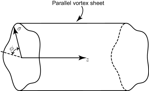
Figure 1: The cylindrical coordinate system: the $z$ axis is parallel to the vortex sheet, the origin is at the centre of the lobed profile and $\phi$ denotes the anticlockwise angle between the radial axis and the horizontal dashed line.

Considering the parallel-flow assumption, we now introduce the cylindrical coordinates $\sigma$, $\phi$ and $z$, as shown in figure 1. In this coordinate frame, the velocity potentials $\psi^{\pm}(\sigma,\phi,z,t)$ satisfy the following Laplace equation:

$$\nabla^{2}\psi^{\pm}(\sigma,\phi,z,t)=0.$$ (9)

Note that we have not yet restricted the profiles of the vortex sheet. It therefore can be of arbitrary geometry, such as rectangular, elliptic or lobed. One can therefore let a general function $\mathcal{R}(\phi)$ denote the radius of the vortex sheet at polar angle $\phi$. Consequently, the profile of the vortex sheet can be specified as

$$\mathcal{F}(\sigma,\phi)=\sigma-\mathcal{R}(\phi)=0.$$ (10)

2.2 The eigenvalue problem

Without losing generality, one may assume

$$\psi^{\pm}=\sum_{m=-\infty}^{\infty}A_{m}E_{m}^{\pm}(\sigma,\phi)\mathrm{e}^{\mathrm{i}\alpha z}e^{-\mathrm{i}\omega t},$$ (11)

where $A_{m}$ are complex constants, $\alpha$ and $\omega$ are the streamwise wavenumber and frequency, respectively. The functions $E_{m}^{\pm}(\sigma,\phi)$ are linearly independent of each other and each pair of them at a given $m$ satisfies both the governing equations and appropriate boundary conditions. The functions $E_{m}^{+}(\sigma,\phi)$ and $E_{m}^{-}(\sigma,\phi)$ are therefore defined in the two-dimensional regions outside ($\sigma>\mathcal{R}(\phi)$) and inside ($\sigma\leq\mathcal{R}(\phi)$) the vortex-sheet profile, respectively, as shown in figure 2.

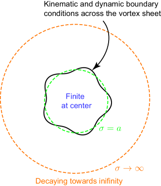
Figure 2: The schematic illustration of the boundary conditions of the stability problem of a parallel lobed vortex sheet.

We choose to normalize the functions $E_{m}^{-}(\sigma,\phi)$ such that for any integer $m$

$$\frac{1}{2\pi}\int_{0}^{2\pi}E_{m}^{-}(a,\phi){E_{m}^{-}}^{\ast}(a,\phi)\mathrm{d}\phi=1,$$ (12)

where $a$, as defined in section 1 and shown in figure 2, is the mean radius of the vortex sheet, which is defined by

$$a=\frac{1}{2\pi}\int_{0}^{2\pi}\mathcal{R}(\phi)\mathrm{d}\phi.$$ (13)

We cannot normalize $E_{m}^{+}(\sigma,\phi)$ according to equation 12, because $E_{m}^{-}(\sigma,\phi)$ and $E_{m}^{+}(\sigma,\phi)$ are not independent. In fact, either the dynamic or the kinematic boundary condition is sufficient to determine $E_{m}^{+}(\sigma,\phi)$ from a given $E_{m}^{-}(\sigma,\phi)$. Therefore, $E_{m}^{+}(\sigma,\phi)$ has to be determined such that for the same mode number $m$, the functions $E_{m}^{+}(\sigma,\phi)$ and $E_{m}^{-}(\sigma,\phi)$ satisfy the boundary conditions. One should note that $E_{m}^{-}(a,\phi)$ are not properly defined within some ranges of $\phi$ (because $E_{m}^{-}(\sigma,\phi)$ is defined for $\sigma\leq\mathcal{R}(\phi)$ and $a>\mathcal{R}(\phi)$ in some ranges of $\phi$, see figure 2 for example). However, they can be naturally defined using analytical continuation, which will become clear at a later stage. Hence, the normalization defined by equation 12 is valid.

Substituting $E_{m}^{\pm}(\sigma,\phi)$ into equation 9 yields the governing equation

$$\left[\frac{\partial^{2}}{\partial\phi^{2}}+\sigma\frac{\partial}{\partial\sigma}\big{(}\sigma\frac{\partial}{\partial\sigma}\big{)}-\alpha^{2}\sigma^{2}\right]E_{m}^{\pm}(\sigma,\phi)=0.$$ (14)

Equation 14 is to be solved subject to appropriate boundary conditions. These are a finite value of $E_{m}^{-}(0,\phi)$, a decay behaviour for $E_{m}^{+}(\sigma,\phi)$ as $\sigma\to\infty$, and the kinematic and dynamic boundary conditions across the vortex sheet (Batchelor & Gill, 1962; Crighton, 1973). Because all the function pairs $E_{m}^{\pm}(\sigma,\phi)$ satisfy both equation 14 and their relevant boundary conditions, they are referred to as the eigenfunctions of this system. The functions $\{E_{m}^{\pm}(\sigma,\phi)\}$ should form a complete set of basis for the Hilbert space determined by the equation 14 and appropriate boundary conditions. The aim of the next section is to calculate these eigenfunctions analytically (without discretizing equation 14 and then solving it numerically).

2.3 The calculation of eigenfunctions

Due to the coupling of $\sigma$ and $\phi$ of the boundary conditions, $E_{m}^{\pm}(\sigma,\phi)$ are not generally expected to be of a separable form. However, in the case of a cylindrical vortex sheet (round jet), the eigenfunctions $E_{m}^{\pm}(\sigma,\phi)$ are known to be separable. Before proceeding to the case of more general vortex sheets, it is instructive to review the characteristics of $E_{m}^{\pm}(\sigma,\phi)$ for a cylindrical vortex sheet.

2.3.1 The solution for a cylindrical vortex sheet

For the cylindrical vortex-sheet flow, the solutions were derived by Batchelor & Gill (1962) and we review them to introduce the notation, and more importantly, these solutions form the basis for analysing more complicated geometries in the following section. The potentials $\psi^{\pm}$ are known to be able to be expanded as

$$\psi^{\pm}=\sum_{n=-\infty}^{\infty}\Psi_{n}^{\pm}(\sigma)\mathrm{e}^{\mathrm{i}n\phi}\mathrm{e}^{\mathrm{i}\alpha z}\mathrm{e}^{-\mathrm{i}\omega t},$$ (15)

where the functions $\Psi_{n}^{\pm}(\sigma)$ satisfy the modified Bessel equation

$$\sigma^{2}\frac{\mathrm{d}^{2}\Psi_{n}^{\pm}}{\mathrm{d}\sigma^{2}}+\sigma\frac{\mathrm{d}\Psi_{n}^{\pm}}{\mathrm{d}\sigma}-\left(\alpha^{2}\sigma^{2}+n^{2}\right)\Psi_{n}^{\pm}=0.$$ (16)

Considering the boundary condition at the centre of the mean flow and at infinity, one can show that

$$\Psi^{-}_{n}(\sigma) =C_{n}^{-}\frac{1}{I_{n}(\alpha a)}I_{n}(\alpha\sigma),$$ (17)

$$\Psi^{+}_{n}(\sigma) =C_{n}^{+}\frac{1}{K_{n}(\alpha a)}K_{n}(\alpha\sigma).$$

where $C_{n}^{-}$ and $C_{n}^{+}$ are arbitrary complex constants and $I_{n}$ and $K_{n}$ are the modified Bessel functions of the first and second kinds, respectively.

Applying the kinematic and dynamic boundary condition on the vortex sheet, one obtains

$$(\omega-\alpha U)\frac{\partial\Psi^{+}_{n}}{\partial\sigma}=\omega\frac{\partial\Psi^{-}_{n}}{\partial\sigma},$$ (18a)

$$\omega\Psi^{+}_{n}=(\omega-\alpha U)\Psi^{-}_{n},$$ (18b)

where use is made of the fact that the function set $\{\mathrm{e}^{\mathrm{i}n\phi}\}$ is orthogonal. For a non-trivial pair of solutions to exist ($C_{n}^{-}C_{n}^{+}\neq 0$), equations 18a and 18b can be rearranged to yield the dispersion relation

$$\Big{(}\frac{\alpha U}{\omega}-1\Big{)}^{2}=\frac{I^{\prime}_{n}(\alpha a)K_{n}(\alpha a)}{I_{n}(\alpha a)K_{n}^{\prime}(\alpha a)}.$$ (19)

In this special case, one can verify that the eigenfunctions, $E_{n}^{+}(\sigma,\phi)$ and $E_{n}^{-}(\sigma,\phi)$, take the separable form of

$$E_{n}^{-}(\sigma,\phi)=\frac{1}{I_{n}(\alpha a)}I_{n}(\alpha\sigma)\mathrm{e}^{\mathrm{i}n\phi},$$ (20)

$$E_{n}^{+}(\sigma,\phi)=\Big{(}1-\frac{\alpha U}{\omega}\Big{)}\frac{1}{K_{n}(\alpha a)}K_{n}(\alpha\sigma)\mathrm{e}^{\mathrm{i}n\phi},$$

where $(1-\alpha U/\omega)$ is obtained from equation 19. Here, $E_{n}^{\pm}(\sigma,\phi)$ take these simple forms because the boundary condition involves no coupling between $\sigma$ and $\phi$ (separable), and therefore these separable solutions are just the eigenfunction of the mathematical problem.

2.3.2 The solution for a vortex sheet of arbitrary geometry

For the case of a non-axisymmetric vortex sheet, the perturbations outside and inside the vortex sheet still remain determined by the Laplace equation. However, the boundary condition is now more complicated. If we were to find an orthogonal coordinate system in which the vortex-sheet profile can be represented by one of the constant coordinate axes, we may be able to find a separable solution. For elliptic profiles, such a coordinate system exists and eigenfunctions of separable form can be obtained (Crighton, 1973). However, it seems rather unlikely to find such a coordinate system for a general profile.

However, in light of the completeness of the orthogonal function set $\{e^{\mathrm{i}n\phi}\}$, we are still able to write the solutions inside and outside the vortex sheet as

$$\psi^{-} =\sum_{-\infty}^{\infty}C^{-}_{n}\frac{1}{I_{n}(\alpha a)}I_{n}(\alpha\sigma)\mathrm{e}^{\mathrm{i}n\phi}\mathrm{e}^{\mathrm{i}\alpha z}\mathrm{e}^{-\mathrm{i}\omega t},$$ (21)

$$\psi^{+} =\sum_{-\infty}^{\infty}C^{+}_{n}\frac{1}{K_{n}(\alpha a)}K_{n}(\alpha\sigma)\mathrm{e}^{\mathrm{i}n\phi}\mathrm{e}^{\mathrm{i}\alpha z}\mathrm{e}^{-\mathrm{i}\omega t},$$

respectively. We must emphasize here that neither the solution $I_{n}(\alpha\sigma)\mathrm{e}^{\mathrm{i}n\phi}/I_{n}(\alpha a)$ nor that $K_{n}(\alpha\sigma)\mathrm{e}^{\mathrm{i}n\phi}/K_{n}(\alpha a)$ is the eigenfunction for this problem, since they do not satisfy the boundary conditions on the vortex sheet (although they satisfy equation 14). However, since they form a complete set, a suitable combination of these separable solutions which satisfies the boundary conditions will be the eigenfunction that we aim to obtain in this section. There may be multiple such combinations, corresponding to eigenfunctions of different orders. For a more compact presentation of the rest of the derivation, let

$$\halign to=0.0pt{\relax\global\advance\@IEEEeqncolcnt by 1\relax\begingroup\csname @IEEEeqnarraycolPREr\endcsname#\relax\relax\relax\relax\relax\relax\relax\relax\relax\relax\csname @IEEEeqnarraycolPOSTr\endcsname\relax\relax\relax\relax\relax\relax\relax\relax\relax\relax\endgroup&\relax\global\advance\@IEEEeqncolcnt by 1\relax\begingroup\csname @IEEEeqnarraycolPREC\endcsname#\relax\relax\relax\relax\relax\relax\relax\relax\relax\relax\csname @IEEEeqnarraycolPOSTC\endcsname\relax\relax\relax\relax\relax\relax\relax\relax\relax\relax\endgroup&\relax\global\advance\@IEEEeqncolcnt by 1\relax\begingroup\csname @IEEEeqnarraycolPREl\endcsname#\relax\relax\relax\relax\relax\relax\relax\relax\relax\relax\csname @IEEEeqnarraycolPOSTl\endcsname\relax\relax\relax\relax\relax\relax\relax\relax\relax\relax\endgroup&\global\advance\@IEEEeqncolcnt by 1\relax\bgroup#\egroup&\global\advance\@IEEEeqncolcnt by 1\relax\hbox to\z@\bgroup\hss#\egroup\cr\hfil$\displaystyle\bar{C}_{n}^{-} $&\hfil$\displaystyle{}={}$\hfil&$\displaystyle C_{n}^{-} \frac{1}{I_{n}(\alpha a)},$\hfil&{{}\vrule width=0.0pt,height=0.0pt,depth=0.0pt}&0.0pt{\hss{\normalcolor(22)}}\cr\penalty 100\vskip 3.0pt\vskip 0.0pt\cr\hfil$\displaystyle\bar{C}_{n}^{+} $&\hfil$\displaystyle{}={}$\hfil&$\displaystyle C_{n}^{+} \frac{1}{K_{n}(\alpha a)}. $\hfil&{\vrule width=0.0pt,height=0.0pt,depth=0.0pt}&0.0pt{\hss{\normalcolor(23)}}\cr}$$

Hence, equation 21 becomes

$$\psi^{-} =\sum_{-\infty}^{\infty}\bar{C}^{-}_{n}I_{n}(\alpha\sigma)\mathrm{e}^{\mathrm{i}n\phi}\mathrm{e}^{\mathrm{i}\alpha z}\mathrm{e}^{-\mathrm{i}\omega t},$$ (24)

$$\psi^{+} =\sum_{-\infty}^{\infty}\bar{C}^{+}_{n}K_{n}(\alpha\sigma)\mathrm{e}^{\mathrm{i}n\phi}\mathrm{e}^{\mathrm{i}\alpha z}\mathrm{e}^{-\mathrm{i}\omega t}.$$

Equation 24 needs to satisfy both the kinematic and dynamic boundary conditions on the vortex sheet, i.e. when $\sigma=\mathcal{R}(\phi)$. The two boundary conditions can be shown to be (see more details in Appendix A),

$$(\omega-\alpha U)\nabla\psi^{+}\cdot\boldsymbol{n}=\omega\nabla\psi^{-}\cdot\boldsymbol{n},$$ (25a)

$$\omega\psi^{+}=(\omega-\alpha U)\psi^{-},$$ (25b)

where $\boldsymbol{n}$ denotes the unit vector normal to the surface of the vortex sheet.

3 Analysis for lobed vortex sheets

Generally, $\mathcal{R}$ can be an arbitrary function of $\phi$. Since we are mostly concerning with the stability of lobed jets, which have a number of identical lobes, it follows that the function $\mathcal{R}$ is a periodic function of $\phi$. This suggests that $\mathcal{R}$ can be readily expanded using Fourier series. As a starting point, we restrict our attention to the simplest case mentioned in section 1, in which case $\mathcal{R}$ is given by

$$\mathcal{R}(\phi)=a\left(1+\epsilon\cos N\phi\right).$$ (26)

For weakly lobed nozzles, $\epsilon\ll 1$, while $\epsilon\sim 0.2$ represents a strongly lobed profile. Figure 3(a) shows some relatively weakly lobed profiles when $\epsilon=0.1$, while figure 3(b) shows some strongly lobed profiles when $\epsilon=0.2$. In either case, we see that $\epsilon$ is a small quantity, and this suggests that the Taylor expansion of a well-behaved function around $\epsilon=0$ should converge sufficiently quickly. For more general lobed profiles, function $\cos N\phi$ can be replaced by a sum over $m$ of terms with $\phi$ dependence $\cos mN\phi$ and $\sin mN\phi$. When $\mathcal{R}$ is given by equation 26, we see that

$$\boldsymbol{n}=\frac{\nabla\mathcal{F}}{\left|\nabla\mathcal{F}\right|},$$ (27)

and

$$\nabla\mathcal{F}=\boldsymbol{e}_{\sigma}+\boldsymbol{e}_{\phi}\frac{a}{\sigma}\epsilon N\sin N\phi,$$ (28)

where $\boldsymbol{e}_{\sigma}$ and $\boldsymbol{e}_{\phi}$ denote the unit vectors in the radial and azimuthal directions, respectively.

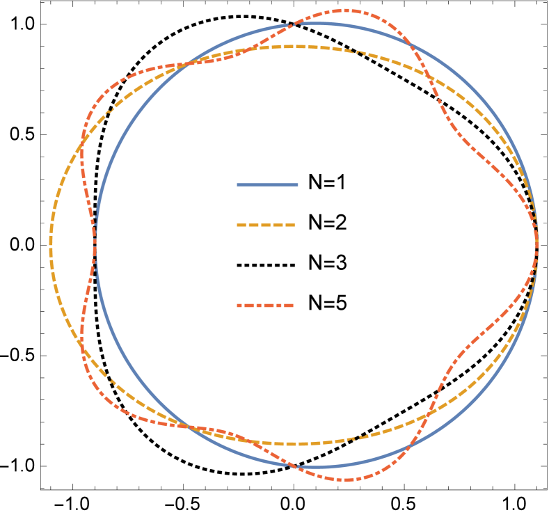
(a) The weakly lobed profiles when $\epsilon=0.1$.

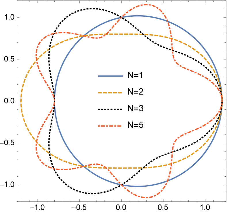
(b) Strongly lobed profiles when $\epsilon=0.2$.

Substituting equations 24, 26 and 27 into equations 25a and 25b yields

$$\begin{dcases}\begin{aligned} \Big{(}1-\frac{\alpha U}{\omega}\Big{)}&\left(\sum_{n=-\infty}^{\infty}\bar{C}_{n}^{+}K_{n}^{\prime}(\alpha a(1+\epsilon\cos N\phi))\mathrm{e}^{\mathrm{i}n\phi}\right.\\ &+\left.\frac{\epsilon N\sin N\phi}{\alpha a(1+\epsilon\cos N\phi)^{2}}\sum_{n=-\infty}^{\infty}\bar{C}_{n}^{+}(\mathrm{i}n)K_{n}(\alpha a(1+\epsilon\cos N\phi))\mathrm{e}^{\mathrm{i}n\phi}\right)=\\ &\left(\sum_{n=-\infty}^{\infty}\bar{C}_{n}^{-}I_{n}^{\prime}(\alpha a(1+\epsilon\cos N\phi))\mathrm{e}^{\mathrm{i}n\phi}\right.\\ &+\left.\frac{\epsilon N\sin N\phi}{\alpha a(1+\epsilon\cos N\phi)^{2}}\sum_{n=-\infty}^{\infty}\bar{C}_{n}^{-}(\mathrm{i}n)I_{n}(\alpha a(1+\epsilon\cos N\phi))\mathrm{e}^{\mathrm{i}n\phi}\right),\end{aligned}\\ \sum_{n=-\infty}^{\infty}\bar{C}_{n}^{+}K_{n}(\alpha a(1+\epsilon\cos N\phi))\mathrm{e}^{\mathrm{i}n\phi}=\Big{(}1-\frac{\alpha U}{\omega}\Big{)}\sum_{n=-\infty}^{\infty}\bar{C}_{n}^{-}I_{n}(\alpha a(1+\epsilon\cos N\phi))\mathrm{e}^{\mathrm{i}n\phi}.\end{dcases}$$ (29)

3.1 Weakly lobed profile

For weakly lobed profile, $\epsilon\ll 1$, therefore we may expand both left and right hand sides of equation 29 around $\epsilon=0$ and keep only the first order without causing too much error. In doing so, the first-order equations can be obtained and, after collecting the terms of the same $\mathrm{e}^{\mathrm{i}n\phi}$, written as

$$\begin{dcases}\begin{aligned} &\sum_{n=-\infty}^{\infty}\left[\bar{C}_{n}^{+}K_{n}^{\prime}(\alpha a)+\bar{C}_{n-N}^{+}\left(K_{n-N}^{\prime\prime}(\alpha a)\frac{\alpha a}{2}+K_{n-N}(\alpha a)\frac{(n-N)N}{2\alpha a}\right)\epsilon\right.\\ &\qquad\qquad\left.\negmedspace{}+C_{n+N}^{+}\left(K_{n+N}^{\prime\prime}(\alpha a)\frac{\alpha a}{2}-K_{n+N}(\alpha a)\frac{(n+N)N}{2\alpha a}\right)\epsilon\right]\mathrm{e}^{\mathrm{i}n\phi}=\\ &\quad\left(\frac{1}{1-\frac{\alpha U}{\omega}}\right)\sum_{n=-\infty}^{\infty}\left[\bar{C}_{n}^{-}I_{n}^{\prime}(\alpha a)+\bar{C}_{n-N}^{-}\left(I_{n-N}^{\prime\prime}(\alpha a)\frac{\alpha a}{2}+I_{n-N}(\alpha a)\frac{(n-N)N}{2\alpha a}\right)\epsilon\right.\\ &\qquad\qquad\quad\left.\negmedspace{}+\bar{C}_{n+N}^{-}\left(I_{n+N}^{\prime\prime}(\alpha a)\frac{\alpha a}{2}-I_{n+N}(\alpha a)\frac{(n+N)N}{2\alpha a}\right)\epsilon\right]\mathrm{e}^{\mathrm{i}n\phi},\end{aligned}\\ \begin{aligned} &\sum_{n=-\infty}^{\infty}\left(\bar{C}_{n}^{+}K_{n}(\alpha a)+\bar{C}_{n-N}^{+}K_{n-N}^{\prime}(\alpha a)\frac{\alpha a}{2}\epsilon+\bar{C}_{n+N}^{+}K_{n+N}^{\prime}(\alpha a)\frac{\alpha a}{2}\epsilon\right)\mathrm{e}^{\mathrm{i}n\phi}=\\ &\quad\Big{(}1-\frac{\alpha U}{\omega}\Big{)}\sum_{n=-\infty}^{\infty}\left(\bar{C}_{n}^{-}I_{n}(\alpha a)+\bar{C}_{n-N}^{-}I_{n-N}^{\prime}(\alpha a)\frac{\alpha a}{2}\epsilon+\bar{C}_{n+N}^{-}I_{n+N}^{\prime}(\alpha a)\frac{\alpha a}{2}\epsilon\right)\mathrm{e}^{\mathrm{i}n\phi}.\end{aligned}\end{dcases}\hphantom{{\normalcolor(30)}}$$ (30)

The above equations can be written in a more compact matrix form, from which the effects of lobed jets can be seen more clearly. Let $\boldsymbol{K}(\alpha a)$ denote the diagonal matrix

$$\boldsymbol{K}(\alpha a)=\textrm{diag}(\cdots K_{-1}(\alpha a),\,K_{0}(\alpha a),\,K_{1}(\alpha a)\cdots),$$ (31)

and let $\boldsymbol{K}_{c}(\alpha a)$ and $\boldsymbol{K}_{s}(\alpha a)$ to be

$$\boldsymbol{K}_{c}(\alpha a)=\begin{bmatrix}[l]\ldots&\ldots\\ \ldots K_{-N-1}(\alpha a)&\ldots K_{N-1}(\alpha a)\ldots\ldots\ldots\\ \ldots\ldots K_{-N}(\alpha a)&\ldots\ldots K_{N}(\alpha a)\ldots\ldots\\ \ldots\ldots\ldots K_{-N+1}(\alpha a)&\ldots\ldots\ldots K_{N+1}(\alpha a)\ldots\\ \ldots\ldots\ldots\ldots&\ldots\ldots\ldots\ldots\\ \end{bmatrix},$$ (32)

and

$$\boldsymbol{K}_{s}(\alpha a)=\begin{bmatrix}[l]\ldots&\ldots\\ \ldots K_{-N-1}(\alpha a)(-N-1)&\ldots-K_{N-1}(\alpha a)(N-1)\ldots\ldots\ldots\\ \ldots\ldots K_{-N}(\alpha a)(-N)&\ldots\ldots-K_{N}(\alpha a)N\ldots\ldots\\ \ldots\ldots\ldots K_{-N+1}(\alpha a)(-N+1)&\ldots\ldots\ldots-K_{N+1}(\alpha a)(N+1)\ldots\\ \ldots\ldots\ldots\ldots&\ldots\ldots\ldots\ldots\\ \end{bmatrix}.$$ (33)

Clearly, each element of the matrices $\boldsymbol{K}(\alpha a)$, $\boldsymbol{K}_{c}(\alpha a)$ and $\boldsymbol{K}_{s}(\alpha a)$ is a function of $\alpha a$, and consequently, these matrices are essentially function matrices with an argument $\alpha a$. We can therefore define the $n$th derivative of a matrix to be the matrix formed by the $n$th derivative of each element function. For example, the first derivative of $\boldsymbol{K}_{c}(\alpha a)$ is

$$\boldsymbol{K}_{c}^{\prime}(\alpha a)=\begin{bmatrix}[l]\ldots&\ldots\\ \ldots K_{-N-1}^{\prime}(\alpha a)&\ldots K_{N-1}^{\prime}(\alpha a)\ldots\ldots\ldots\\ \ldots\ldots K_{-N}^{\prime}(\alpha a)&\ldots\ldots K_{N}^{\prime}(\alpha a)\ldots\ldots\\ \ldots\ldots\ldots K_{-N+1}^{\prime}(\alpha a)&\ldots\ldots\ldots K_{N+1}^{\prime}(\alpha a)\ldots\\ \ldots\ldots\ldots\ldots&\ldots\ldots\ldots\ldots\\ \end{bmatrix}.$$ (34)

If one replaces the modified Bessel function of the second kind $K_{n}(\alpha a)$, in matrices $\boldsymbol{K}(\alpha a)$, $\boldsymbol{K}_{c}(\alpha a)$ and $\boldsymbol{K}_{s}(\alpha a)$, with function $I_{n}(\alpha a)$, the matrices $\boldsymbol{I}(\alpha a)$, $\boldsymbol{I}_{c}(\alpha a)$ and $\boldsymbol{I}_{s}(\alpha a)$ can be similarly defined. Upon defining the vector

$$\boldsymbol{\bar{C}^{\pm}}=\left[\ldots,\bar{C}_{-n}^{\pm},\ldots,\bar{C}_{0}^{\pm},\ldots,\bar{C}_{n}^{\pm},\ldots\right]^{T},$$ (35)

where $[\ \,]^{T}$ denotes the transpose of matrix $[\ \,]$, equation 30 can be readily written as

$$\begin{dcases}&\begin{aligned} \Big{(}1-\frac{\alpha U}{\omega}\Big{)}&\left[\boldsymbol{K}^{\prime}(\alpha a)+\epsilon\left(\boldsymbol{K}^{\prime\prime}_{c}(\alpha a)\frac{\alpha a}{2}+\boldsymbol{K}_{s}(\alpha a)\frac{N}{2\alpha a}\right)\right]\boldsymbol{\bar{C}}^{+}=\\ &\quad\quad\quad\left[\boldsymbol{I}^{\prime}(\alpha a)+\epsilon\left(\boldsymbol{I}^{\prime\prime}_{c}(\alpha a)\frac{\alpha a}{2}+\boldsymbol{I}_{s}(\alpha a)\frac{N}{2\alpha a}\right)\right]\boldsymbol{\bar{C}}^{-},\end{aligned}\\ &\left[\boldsymbol{K}(\alpha a)+\epsilon\boldsymbol{K}_{c}^{\prime}(\alpha a)\frac{\alpha a}{2}\right]\boldsymbol{\bar{C}}^{+}=\Big{(}1-\frac{\alpha U}{\omega}\Big{)}\left[\boldsymbol{I}(\alpha a)+\epsilon\boldsymbol{I}_{c}^{\prime}(\alpha a)\frac{\alpha a}{2}\right]\boldsymbol{\bar{C}}^{-}.\end{dcases}$$ (36)

Equation 36 represents the dispersion relation for the considered lobed jet to the first-order accuracy. It is worth noting that both $\boldsymbol{K}(\alpha a)$ and $\boldsymbol{I}(\alpha a)$ are diagonal matrices. Therefore, in the case of $\epsilon=0$, i.e. the axisymmetric vortex sheet, equation 36 represents a set of decoupled dispersion relation equations. Consequently, stability analysis can be performed for each mode individually and the results are identical to those obtained by Batchelor & Gill (1962), as shown above. When $\epsilon\neq 0$, the equations governing the dispersion relations are coupled equations, hence the equations must be solved together.

Before proceeding to solve these equations, it is informative to examine how lobed vortex-sheet profiles affect the characteristic matrices. Firstly, one can see that the coupling only occurs between modes $n$, $n-N$ and $n+N$. Had we included higher order terms ($\epsilon^{2},\epsilon^{3}\dots$), the coupling would involve modes $n\pm kN$ ($k=0,\pm 1,\pm 2\dots$). This shows that the lobed profile affects the instability waves by modulating them with its own periodicity. Secondly, the modulating effects occur in two ways: modifying the radial length scales and changing the normal directions of vortex sheet. The effects of modifying the radial length scales are represented by the $\boldsymbol{K}_{c}^{(i)}(\alpha a)$ and $\boldsymbol{I}_{c}^{(i)}(\alpha a)$ matrices ($i$ here denotes the $i$th derivative). Take the strongly-lobed profile of $N=2$, as shown in figure 3(b), as an example. At such a large value of $\epsilon$, the lobe profile resembles that of an elliptic vortex sheet. Hence, the radial length scales of the major and the minor axes are different. It is known that this causes different behaviour for instability waves orientated with different axes (Crighton, 1973). In the dynamic boundary conditions shown in equation 36, the $\boldsymbol{K}_{c}^{\prime}(\alpha a)$ and $\boldsymbol{I}_{c}^{\prime}(\alpha a)$ terms account for the different length scales (to the first order accuracy) and ensure pressure is continuous across the vortex sheet. The $\boldsymbol{K}_{s}(\alpha a)$ and $\boldsymbol{I}_{s}(\alpha a)$ matrices, on the other hand, account for changing of the restrictions on the normal perturbation velocities across the vortex sheet. Equation 25a shows that it is the normal (to the vortex sheet) perturbation velocities that have to satisfy the jump condition. From equation 28 it is evident that the use of lobed nozzles can significantly change the local normal directions of the vortex sheet and hence the instability characteristics. Also, it is clear from equation 28 that the normal direction changes more pronouncedly as $N$ increases.

To solve equation 36, we write the two matrix equations in a more compact form as

$$\Big{(}1-\frac{\alpha U}{\omega}\Big{)}\boldsymbol{K}_{k}\bar{\boldsymbol{C}}^{+}=\boldsymbol{I}_{k}\bar{\boldsymbol{C}}^{-},$$ (37a)

$$\boldsymbol{K}_{d}\bar{\boldsymbol{C}}^{+}=\Big{(}1-\frac{\alpha U}{\omega}\Big{)}\boldsymbol{I}_{d}\bar{\boldsymbol{C}}^{-}.$$ (37b)

The definitions of $\boldsymbol{K}_{k}$, $\boldsymbol{I}_{k}$, $\boldsymbol{K}_{d}$ and $\boldsymbol{I}_{k}$ should be obvious when compared with equation 36, and from now on we omit the argument $\alpha a$ of relevant matrices for brevity. Equations 37a and 37b are in terms of $\boldsymbol{\bar{C}^{\pm}}$, it is necessary to obtain an equation in terms of $\boldsymbol{C^{\pm}}$ ($\boldsymbol{C^{\pm}}$ is the column vector with elements $C_{n}^{\pm}$ rather than $\bar{C}_{n}^{\pm}$). This is because $C_{n}^{\pm}$ are the coefficients in front of normalized functions, and hence represent the proper amplitudes of their corresponding eigenfunctions. On the other hand, $\bar{C}_{n}^{\pm}$ denote the non-normalized coefficients, hence their values would depend on the amplitudes of their eigenfunctions. For example, because the value of $I_{n}(\alpha a)$ at a fixed $\alpha a$ decreases exponentially as $n$ increases, $\bar{C}_{n}^{-}$ would have to increase exponentially as $n$ increases in order to ensure a physically meaningful result is obtained. This is clearly not suitable for any numerical evaluations at a later stage. Therefore, it is essential to rewrite the above two equations in terms of $C^{\pm}$. It is straightforward to show $\boldsymbol{C}^{+}=\boldsymbol{K}\boldsymbol{\bar{C}}^{+}$ and $\boldsymbol{C}^{-}=\boldsymbol{I}\boldsymbol{\bar{C}}^{-}$. Since both $\boldsymbol{I}$ and $\boldsymbol{K}$ are diagonal matrices, it is trivial to calculate their inverse matrices $\boldsymbol{I}^{-1}$ and $\boldsymbol{K}^{-1}$. Equations 37a and 37b can be easily changed to

$$\Big{(}1-\frac{\alpha U}{\omega}\Big{)}\widetilde{\boldsymbol{K}}_{k}\boldsymbol{C}^{+}=\widetilde{\boldsymbol{I}}_{k}\boldsymbol{C}^{-},$$ (38a)

$$\widetilde{\boldsymbol{K}}_{d}\boldsymbol{C}^{+}=\Big{(}1-\frac{\alpha U}{\omega}\Big{)}\widetilde{\boldsymbol{I}}_{d}\boldsymbol{C}^{-},$$ (38b)

where $\widetilde{\boldsymbol{K}}_{k}=\boldsymbol{K}_{k}\boldsymbol{K}^{-1}$, $\widetilde{\boldsymbol{K}}_{d}=\boldsymbol{K}_{d}\boldsymbol{K}^{-1}$, $\widetilde{\boldsymbol{I}}_{k}=\boldsymbol{I}_{k}\boldsymbol{I}^{-1}$, $\widetilde{\boldsymbol{I}}_{d}=\boldsymbol{I}_{d}\boldsymbol{I}^{-1}$. These tilde matrices can be calculated quickly since both $\boldsymbol{I}^{-1}$ and $\boldsymbol{K}^{-1}$ are diagonal.

From equation 38b, we see that

$$\boldsymbol{C}^{+}=\Big{(}1-\frac{\alpha U}{\omega}\Big{)}\widetilde{\boldsymbol{K}}_{d}^{-1}\widetilde{\boldsymbol{I}}_{d}\boldsymbol{C}^{-}.$$ (39)

Substituting equation 39 into equation 38a, we have

$$\Big{(}1-\frac{\alpha U}{\omega}\Big{)}^{2}\widetilde{\boldsymbol{K}}_{k}\widetilde{\boldsymbol{K}}_{d}^{-1}\widetilde{\boldsymbol{I}}_{d}\boldsymbol{C}^{-}=\widetilde{\boldsymbol{I}}_{k}\boldsymbol{C}^{-}.$$ (40)

Upon multiplying $\widetilde{\boldsymbol{I}}_{k}^{-1}$ on both sides of equation 40 and defining $\boldsymbol{A}=\widetilde{\boldsymbol{I}}_{k}^{-1}\widetilde{\boldsymbol{K}}_{k}\widetilde{\boldsymbol{K}}_{d}^{-1}\widetilde{\boldsymbol{I}}_{d}$, we obtain the following eigenvalue problem

$$\boldsymbol{A}\boldsymbol{C}^{-}=\lambda\boldsymbol{C}^{-},$$ (41)

where

$$\lambda=\Big{(}1-\frac{\alpha U}{\omega}\Big{)}^{-2}.$$ (42)

The matrix $\boldsymbol{A}$ is of an infinite dimension. In order to calculate its eigenvalues in practical cases, we may drop all the modes higher than $M$ (and less than $-M$). Though we expect results to become inaccurate for large modes close to $M$, it may yield satisfactory results for relatively low-order modes when $M$ is taken to be adequately large. These low-order modes are of our primary interest in this study, since high-order modes vanish sufficiently quickly according to experimental results (Tinney & Jordan, 2008). Besides, the vortex-sheet assumption would fail for high-order modes anyway. By truncating high-order terms, we obtain a matrix of $(2M+1)\times(2M+1)$, and there are $2M+1$ eigenvalues (degenerate eigenvalues are counted more than once) and their corresponding eigenvectors. For each obtained eigenvector $\boldsymbol{C}^{-}$, we can obtain the corresponding $\boldsymbol{C}^{+}$ easily from equation 39. The fact that the non-zero eigenvector $\boldsymbol{C}^{-}$ satisfies equation 41 entails that the non-trivial velocity potential $\psi^{-}$, determined by $\boldsymbol{C}^{-}$, and the corresponding $\psi^{+}$, determined by $\boldsymbol{C}^{+}$, satisfy both the kinematic and dynamic boundary conditions on the vortex sheet. Therefore, each eigenvector represents an eigenfunction of the lobed problem, i.e.

$$E_{n}^{-}(\sigma,\phi)=\sum_{n=-\infty}^{\infty}C_{n}^{-}\frac{1}{I_{n}(\alpha a)}I_{n}(\alpha\sigma)\mathrm{e}^{\mathrm{i}n\phi},$$ (43)

$$E_{n}^{+}(\sigma,\phi)=\sum_{n=-\infty}^{\infty}C_{n}^{+}\frac{1}{K_{n}(\alpha a)}K_{n}(\alpha\sigma)\mathrm{e}^{\mathrm{i}n\phi}.$$

One can readily verify that, when $\boldsymbol{C}^{-}$ is normalized such that $(\boldsymbol{C}^{-})^{\ast T}\boldsymbol{C}^{-}=1$ and $\boldsymbol{C}^{+}$ is obtained from the dynamic boundary conditions shown in equation 39, both $E_{n}^{-}(\sigma,\phi)$ and $E_{n}^{+}(\sigma,\phi)$ are normalized as described in Section 2.2.

3.2 The mode labelling strategy

When $\epsilon=0$, there is a well-defined mode number for each mode. For example, mode $n$ can be defined as the eigenvector

$$\boldsymbol{C}^{-}=\left[\ldots 0,\ldots,0,\ldots,C_{n}^{-}=1,\ldots\right]^{T}.$$ (44)

When $\epsilon\neq 0$, however, the eigenvector does not posses this simple property. Instead, the resulting eigenvector has other non-vanishing elements besides $C_{n}^{-}$. We need to develop an unambiguous strategy to label the eigen-modes.

We can show that the eigenvector $\boldsymbol{C}^{-}$ can be always defined as either symmetric or antisymmetric (with respect to the element of index $0$). This is due to the rotationally symmetric property possessed by the matrix $\boldsymbol{A}$, and for brevity we have placed detailed derivation in Appendix B.

Based on this property, we define an eigenvector to have a mode number $n$ if it is symmetric and

$$||\boldsymbol{C}^{-}-\boldsymbol{G}||=\sqrt{\sum_{j=-M}^{M}(|C_{j}^{-}|-G_{j})^{2}}$$ (45)

yields a minimum value when $n$ varies from $-M$ to $M$ and

$$\boldsymbol{G}=\left[\ldots,g_{-n}=\sqrt{2}/2,\ldots,0,\ldots,g_{n}=\sqrt{2}/2,\ldots\right]^{T},$$ (46)

where $g_{n}$ is the element of the gauge vector $\boldsymbol{G}$. For anti-symmetric eigenvectors we label it as $-n$ in a similar manner. For $n=0$, it is trivial to label its mode number and it can be shown that it is a symmetric vector. By labelling the eigenvectors in this way, equation 43 implies that all nonnegative eigenfunctions are even functions of $\phi$ and negative ones odd.

In the following analysis, the mode number for the obtained eigenfunction is designated according to the above conventions. Then for each mode $n$, we can calculate its corresponding eigenvalue $\lambda_{n}$ at a given value of $\alpha a$. The complex frequency $\omega$ can be directly obtained from $\lambda_{n}$ according to equation 42. This complex number determines both the growth rate and the convection velocity of its corresponding instability wave. Therefore, by varying the values of $\epsilon$ and $N$, one can easily examine how different lobed geometry changes both the growth rate and convection velocity of instability waves of different mode numbers.

3.3 Strongly lobed nozzle

For strongly lobed nozzles, e.g. $\epsilon\sim 0.2$, it is necessary to include high-order terms $\epsilon^{n}$. Luckily this is not a difficult extension, and all the aforementioned procedures used to solve the eigenvalue problem remain the same. It suffices to find the high-order coefficient matrices and add them into equation 36, i.e.

$$\boldsymbol{K}_{k} =\boldsymbol{K}^{\prime}(\alpha a)+\epsilon\Big{(}\boldsymbol{K}^{\prime\prime}_{c}(\alpha a)\frac{\alpha a}{2}+\boldsymbol{K}_{s}(\alpha a)\frac{N}{2\alpha a}\Big{)}+\epsilon^{2}\Big{(}\dots\Big{)}+\cdots,$$ (47)

$$\boldsymbol{I}_{k} =\boldsymbol{I}^{\prime}(\alpha a)+\epsilon\Big{(}\boldsymbol{I}^{\prime\prime}_{c}(\alpha a)\frac{\alpha a}{2}+\boldsymbol{I}_{s}(\alpha a)\frac{N}{2\alpha a}\Big{)}+\epsilon^{2}\Big{(}\dots\Big{)}+\cdots,$$

$$\boldsymbol{K}_{d} =\boldsymbol{K}(\alpha a)+\epsilon\boldsymbol{K}_{c}^{\prime}(\alpha a)\frac{\alpha a}{2}+\epsilon^{2}(\dots)+\cdots,$$

$$\boldsymbol{I}_{d} =\boldsymbol{I}(\alpha a)+\epsilon\boldsymbol{I}_{c}^{\prime}(\alpha a)\frac{\alpha a}{2}+\epsilon^{2}(\dots)+\cdots.$$

It is worth noting that incorporating higher-order terms does not invalidate the matrix $\boldsymbol{A}$ being rotationally symmetric, hence all the previous conclusions about its eigenvectors still remain valid. Due to the nature of higher-order modified Bessel functions, expanding them around $\alpha a$ results in a slow convergence when $\epsilon$ is large. Therefore, the number of high-order terms needed increases quickly as $\epsilon$ increases. It also increases when we increase the value of $M$. However, this problem can be overcome by expanding properly scaled modified Bessel functions. Since in this study we only need a relatively small $M$, and the extension of incorporating more higher-order terms can be promptly automated using computer programming, it is not strictly necessary to expand the scaled modified Bessel functions instead. For example, a MATLAB code has been developed that can automatically incorporate as many orders of terms as needed. Due to its analytical nature, the computation is very fast. For example, a comprehensive eigenvalue analysis of order $10$ with $M=20$ takes less than $50$ milliseconds. All the results shown in the following sections are obtained by incorporating higher-order terms to the order of $10$ ($\epsilon^{10}$) and with $M=20$. A convergence analysis, to be shown in section 4.1, shows that this is much more than necessary.

4 Validation and Results

As mentioned in the preceding section, both the temporal growth rate and convection velocity of the instability waves can be readily obtained from equation 42. In this section, we present the rich results obtained from this procedure.

4.1 Convergence analysis

We first examine the convergence characteristics of this new method when the order of accuracy $m$ ($\epsilon^{m}$) and $M$ change. To separate the effects of $m$ and $M$, we can fix $M$ and vary the values of $m$ and then vice versa. For brevity, we choose to present the convection velocity and temporal growth rate of mode $1$ instability wave and fix the number of lobes $N=2$.

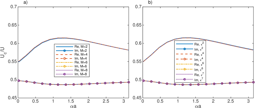
Figure 4: The convergence of the temporal growth rate and convection velocity for the mode $1$ instability wave when $N=2$ and $\epsilon=0.1$: a) the order of accuracy is fixed at $\epsilon^{10}$ while $M$ varies from $2$ to $8$; b) $M$ is fixed to be $20$ while the order of accuracy varies from $\epsilon^{2}$ to $\epsilon^{7}$.

We first show the results for a relatively small penetration ratio, i.e. $\epsilon=0.1$. The results are shown in figure 4. For a compact presentation, we define a complex number $U_{c}\equiv\omega/\alpha$. Therefore, the real part of $U_{c}$ denotes the convection velocity while the imaginary part represents the temporal growth rate. Figure 4 shows the real and imaginary parts of $U_{c}$, respectively.

Figure 4(a) shows the results when $m=10$ and $M$ varies from $2$ to $8$. One can see that both the growth rates and convection velocities are hardly distinguishable. This shows that, for a small value of $\epsilon\approx 0.1$, $M=2$ is essentially sufficient, at least for the mode number $1$. Of course we would need a slightly larger value of $M$ if we were to consider higher-order modes. But this increase in $M$ is likely to be on a small scale, because we are only interested in low-order modes as only those are physically relevant in experiments. Figure 4(b) shows the results when $M$ is fixed at $20$ and $m$ varies from $2$ to $7$. Similar to figure 4(a), the lines are nearly on top of each other. This shows that for $\epsilon\approx 0.1$, a second-order accuracy is sufficient for a good convergence.

As mentioned in section 3.3, due to the nature of the modified Bessel functions, the number of high-order $\epsilon^{n}$ terms needed increases quickly as $\epsilon$ increases. To show that $M=20$ and $m=10$ is also sufficient for a large value of $\epsilon$, we present the convergence characteristics of this analysis when $\epsilon=0.2$ in figure 5.

Figure 5(a) shows the results when $m=10$ and $M$ varies from $2$ to $8$. We can see that there is an observable difference between the convection velocities calculated using $M=2$ and $M=4$. However, there is little change between the results for $M=4$ and $M=8$. This shows that for strongly lobed geometry at $\epsilon\approx 0.2$, $M$ must be at least $4$. On the other hand, it is interesting to see that the temporal growth rate is much less sensitive to the change in $M$ than the convection velocity. Figure 5(b) similarly shows the results for a fixed number $M=20$ and a varying $m$. The observation is similar to figure 5(a), and it shows that for $\epsilon\approx 0.2$, a high order accuracy up to $\epsilon^{4}$ or $\epsilon^{6}$ is recommended. In summary, the results in this section show that $M=20$ and $n=10$ can ensure the obtained eigen-solutions are well converged.

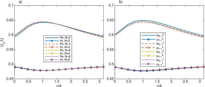
Figure 5: The convergence of the temporal growth rate and convection velocity for the mode $1$ instability wave when $N=2$ and $\epsilon=0.2$: a) the order of accuracy is fixed at $\epsilon^{10}$ while $M$ varies from $2$ to $8$; b) $M$ is fixed to be $20$ while the order of accuracy varies from $\epsilon^{2}$ to $\epsilon^{7}$.

4.2 Validation

Section 4.1 merely shows that $M=20$ and $n=10$ are sufficient for a good convergence. A converged solution, however, does not always imply a correct one. Consequently, before presenting any results, it is necessary to validate this new analysis framework. Luckily, it is very straightforward to do so. Since the entire analysis is devoted to calculating the eigenfunctions that satisfy both the kinematic and dynamic boundary conditions on the vortex sheet, we can examine the obtained eigenfunctions to ensure that they do indeed satisfy the two boundary conditions. More precisely, we can show that for each pair of eigenfunctions obtained above, we have, on the vortex sheet,

$$(1-\alpha U/\omega)\nabla E_{m}^{+}(\sigma,\phi)\cdot\boldsymbol{n}=\nabla E_{m}^{-}(\sigma,\phi)\cdot\boldsymbol{n},$$ (48a)

$$1/(1-\alpha U/\omega)E_{m}^{+}(\sigma,\phi)=E_{m}^{-}(\sigma,\phi).$$ (48b)

The obtained eigen-solution will automatically satisfy the Laplace equation both inside and outside the vortex sheet, because we have chosen to expand the eigen-solution using a set of basis functions which are already the solutions to the Laplace equation. Therefore, it is sufficient to validate the method by only verifying that the boundary conditions are met. In the rest of this paper, we refer to both sides of equation 48a and 48b as the normalized normal perturbation velocity and pressure, respectively. One can first evaluate both sides of the above two equations on the vortex sheet (similar to equation 29) and plot them together. If the results are accurate, the normalized normal perturbation velocity and pressure would collapse. Since the eigenvector of mode $n$ ($n\geq 0$) is symmetric, if it is also real, then it is effortless to show that the imaginary parts of $E_{n}^{-}(\sigma,\phi)$ are strictly zero. Similarly, the real parts of $E_{-n}^{-}(\sigma,\phi)$ also vanish when the eigenvector of mode $-n$ is real. For the results shown in this paper, all the eigenvectors are real. Therefore, for mode $n$ ($n\geq 0$), it suffices to plot only the real parts of equations 48a and 48b. Likewise, for mode $-n$ ($n>0$), one only needs to plot the imaginary parts. For the sake of brevity, we only show the results for modes $-2$ and $2$. All other modes of interest have similar level of agreement. The results are shown in figure 6.

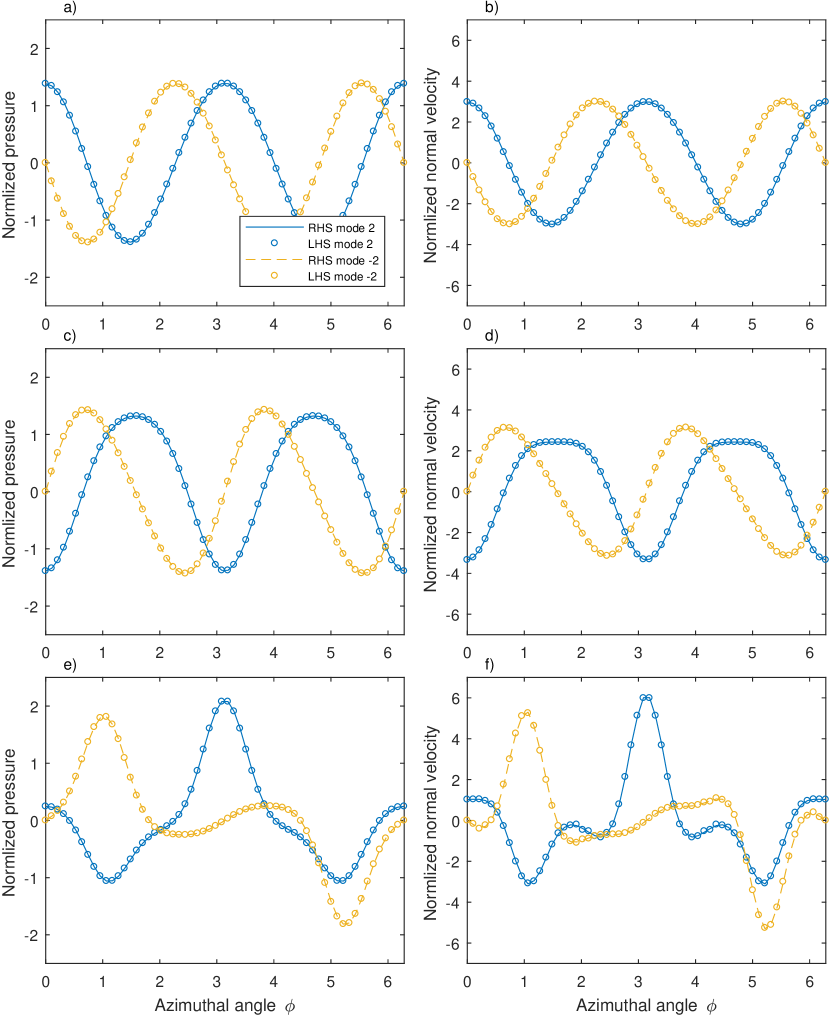
Figure 6: The match validation of the dynamic (left) and kinematic (right) boundary conditions for the eigenfunctions of modes $\pm 2$ when the number of lobes $N$ are different: a, b) $N=1$; c, d) $N=2$; e, f) $N=3$. The normalized wavenumber is $\alpha a=1$ and the lobed profile has a penetration ratio $\epsilon=0.1$.

Figure 6 shows how the boundary conditions are satisfied by the eigenfunctions of modes $\pm 2$. These results are obtained with $\alpha a=1$ and $\epsilon=0.1$. Figures 6(a) and 6(b) show the matches of the left and right sides of equations 48b and 48a, respectively, when the number of lobes is $N=1$. From figure 3(a), one can see that when $N=1$, the lobed profile is not very significantly different from the axisymmetric one. The single lobe merely causes a displacement of the profile centre of the circular vortex sheet. Therefore, one expects that the dynamics of instability waves shall remain largely unchanged. Figure 6(a,b) indeed confirms this. Modes $2$ and $-2$ resemble those of an axisymmetric vortex sheet in every aspect. When $N$ increases to $2$, the effects of lobes are more pronounced, as shown in figure 6(c,d). In particular, the symmetric (with respect to $\phi=0)$ eigenfunction shown in figure 6(d) starts to deviate from the normal $-\cos 2\phi$ function, with its peak somewhat flattened. The mode $-2$, on the other hand, remains largely similar to $\sin 2\phi$. When $N$ increases to $3$, both modes $2$ and $-2$ respond to the change of vortex-sheet geometry and change their shapes significantly.

It is, however, worth noting that, for $N=1$ and $N=2$, the eigenvalues $\lambda_{2}\neq\lambda_{-2}$. Therefore, both $E_{2}^{-}(\sigma,\phi)$ and $E_{-2}^{-}(\sigma,\phi)$ have a standing wave pattern with respect to $\phi$ and they cannot be combined to produce a travelling wave. However, for $N=3$ we find that $\lambda_{2}=\lambda_{-2}$. Therefore, a travelling-wave pattern can be obtained. The important observation is that, for all the six figures, exceptionally good matches of the pressure and normal velocity across the layer of vortex sheet are achieved. The excellent agreement seen from figure  6 shows that the analytical framework developed in this section works exceptionally well, at least for the low-order modes like those we have just shown.

4.3 The effects of lobed profiles on the convection velocity and growth rate of instability waves

Having validated the analytical framework, we are now in a position to examine the effects of lobed profiles on the convection velocity and growth rate of instability waves. In the rest of this section, we plot both quantities versus the normalized frequency $\alpha a$, for lobed profiles of different geometry.

We start from showing results for mode $0$. These are shown in figure 7. Figure 7(a) shows the convection velocity and growth rate for a single-lobe profile. To facilitate a direct comparison to the results of a cylindrical vortex sheet, both quantities are plotted when $\epsilon=0$ first. As can be seen, when the frequency $\alpha a$ increases, the normalized convection velocity ($\Re{U_{c}/U}$) decreases from unity to around $0.5$, whereas the normalized growth rate ($\Im{U_{c}/U}$) increases from $0$ to the same limit value. However, it shows that a single lobe does not cause any observable changes to the characteristics of mode $0$ at all frequencies, no matter what value of $\epsilon$ is used. The same conclusion can be reached for $N=2$, which is shown in figure 7(b). Increasing the number of lobes to $3$, however, starts to cause a slightly larger convection velocity and a marginally lower growth rate. These results are shown in figure 7(c), from which we see that the changes are only observable at high frequencies. However, they become more pronounced when the penetration ratio $\epsilon$ increases. The increase of the convection velocity and the reduction of the temporal growth rate, caused by lobed vortex-sheet profiles, are more evident when the number of lobes is increased to $5$. As shown in figure 7(d), at high frequencies ($\alpha a>1.5$), a large penetration ratio results in an effective rise of the convection velocity and a less effective drop of the growth rate. However, one should note that although these changes are observable, they are not in any way significant.

The fact that serrations increase the convection velocity and reduce growth rates of mode $0$ is in accord with the findings of Lajús Jr. et al. (2015) and Sinha et al. (2016). However, it should be noted that in the work of Sinha et al. (2016), there also exists a low-frequency band where the spatial convection velocity is slightly reduced. Such a difference might be caused by the difference between temporal and spatial analysis, the difference in jet mean flow profiles or the difference in the shear layer thickness.

Figure 7 shows that instability waves of mode $0$ are not very sensitive to either the number of lobes or the penetration ratio. Figure 8, however, shows a different story for mode $1$. The eigenfunctions corresponding to mode $1$ are even functions of $\phi$. Figure 8(a) still indicates that a single lobe does not noticeably change the characteristics of the mode $1$ instability waves. This is somewhat expected. Because, as we observed before, one single lobe merely causes a displacement of the profile’s geometrical centre. Therefore, the physics should more or less stay the same as that of an axisymmetric vortex-sheet. This is consistent with the results shown in figure 8(a).

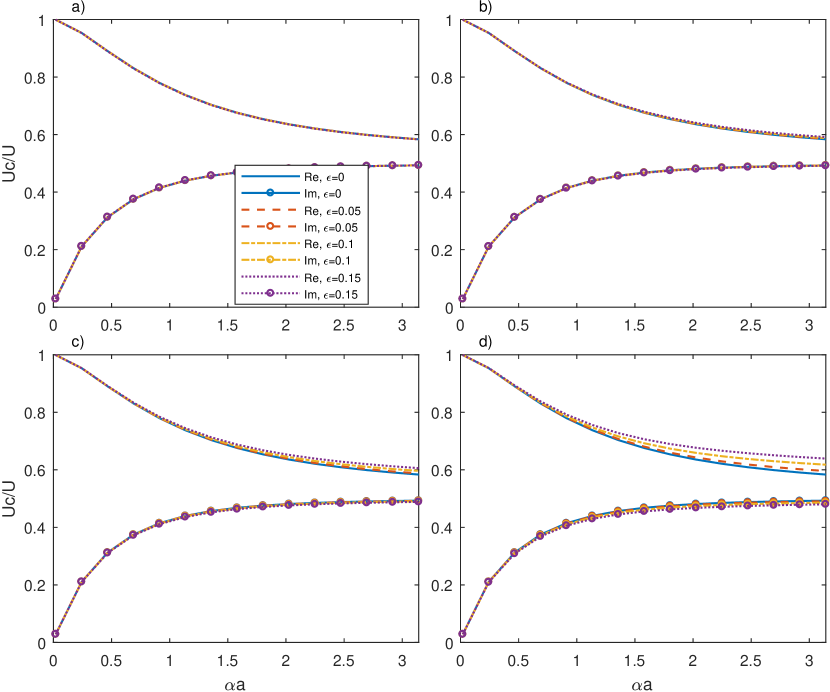
Figure 7: The convection velocity and growth rate of the mode $0$th jet instability waves for vortex sheets of different lobed geometry: a) $N=1$; b) $N=2$; c) $N=3$; d) $N=5$.

However, figure 8(b) shows that the use of $2$ lobes leads to a pronounced increase of the convection velocity, and a slight decrease of the temporal growth rate. In contrast to those shown in figure 7, the increase of the convection velocity is more marked at low frequencies. Similarly, increasing $\epsilon$ results in a stronger rise of the convection velocity. It is very interesting o note that the rise of the convection velocity is nearly linear with respect to $\epsilon$. The decrease of the temporal growth rate, however, is most notable in the intermediate frequency range, and the maximum decrease is very small. Figure 8(c) shows the results for $N=3$. Compared to figure 8(b), the effects of lobes on both the convection velocity and the growth rate appear to be more effective. The most pronounced change, however, occurs when $N$ increases to $5$, as shown in figure 8(d). Again, these results are consistent with the findings of Sinha et al. (2016). The dependence of both the convection velocity and the temporal growth rate on $\epsilon$ appears to linear. But the relative change of the former is significantly larger than that of the latter.

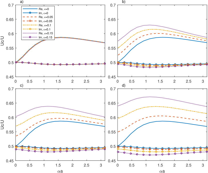
Figure 8: The convection velocity and growth rate of the mode $1$ jet instability waves for vortex sheets of different lobed geometry: a) $N=1$; b) $N=2$; c) $N=3$ d) $N=5$.

Figure 9 presents the results for the mode $-1$. The eigenfunctions are odd functions of $\phi$. Still, figure 9(a) does not show observable changes when $\epsilon$ increases. However, zooming in this figure, one can see that the convection velocity is weakly increasing as $\epsilon$ increases, and this is opposite to that observed in figure 8(a)! This different behaviour is because $\lambda_{1}$ is not identical to $\lambda_{-1}$ any more. Therefore, the odd and even eigenfunctions are now independent of each other and they change in opposite ways as $\epsilon$ increases. If figures 9(a) and 8(a) are too similar to each other to make this trend clear, figure 9(b) makes it much more evident.

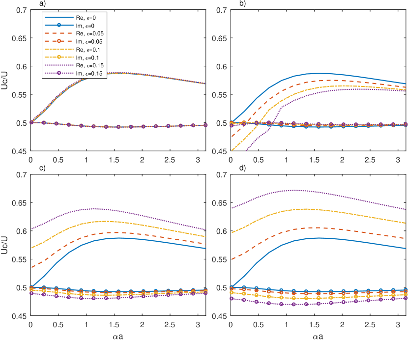
Figure 9: The convection velocity and growth rate of the mode $-1$ jet instability waves for vortex sheets of different lobed geometry: a) $N=1$; b) $N=2$; c) $N=3$; d) $N=5$.

The number of lobes is now $2$, and the lobed profile is approximately elliptic. Instead of obtaining higher convection velocities, increasing $\epsilon$ from $0$ now results in increasingly smaller convection velocities. The temporal growth rate, on the other hand, starts to drop at low frequencies ($\alpha a<0.5$), but gradually changes to increase at high frequencies, although both are on a small scale. The different eigenvalues of modes $\pm 1$, hence distinctive characteristics of instability waves of modes $\pm 1$, are consistent with the analytical results obtained by Crighton (1973) for elliptic vortex sheets and also agree with the findings in the spatial stability analysis carried out by Kopiev et al. (2004) (because the mode number $1$ is a half of the number of lobes $N=2$). Figure 9(c,d) shows the results for $N=3$ and $N=5$, respectively. One can easily verify that they are identical to those shown in figure 8(c, d). This is because, for both $N=3$ and $N=5$, the eigenvalues $\lambda_{n}$ remain identical to $\lambda_{-n}$. As discussed in Section 4.2, this also implies that azimuthally travelling waves can exist, in contrast to the case of $\lambda_{n}\neq\lambda_{-n}$, where only azimuthally standing waves are allowed.

Figure 10 shows results for the instability waves of mode $2$. Figure 10(a) is for $N=1$. We expect little change caused by one single lobe, and this is demonstrated clearly by the figure.

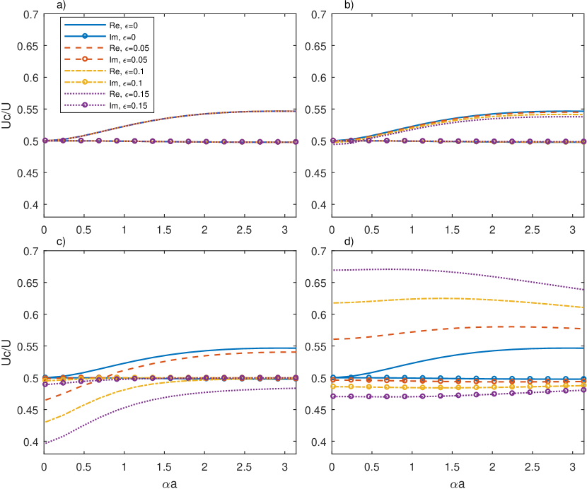
Figure 10: The convection velocity and growth rate of the mode $2$ jet instability waves for vortex sheets of different lobed geometry: a) $N=1$; b) $N=2$; c) $N=3$; d) $N=5$.

The results for $N=2$ are shown in figure 10(b). The mode $2$ instability waves have increasingly lower convection velocities when $\epsilon$ increases. But the changes are very small. The changes of the temporal growth rate are nearly unobservable. However, using $3$ lobes can still effectively reduce the convection velocity while marginally altering the temporal growth rate of the mode $2$ instability waves. Like all the results we have reported, the use of $5$ lobes is the most effective way of increasing the convection velocity and decreasing the temporal growth rate. Figure 11 shows the results for the mode $-2$ instability waves. Figure 11(a) exhibits expected behaviour for a lobed profile of $N=1$. Figure 11(b) shows a very slight increase of the convection velocity and no change to the temporal growth rate. We emphasize again that this is due to $\lambda_{n}\neq\lambda_{-n}$. Figures 11(c) and 11(d) are identical to figures 10(c) and 10(d) respectively because of identical eigenvalues.

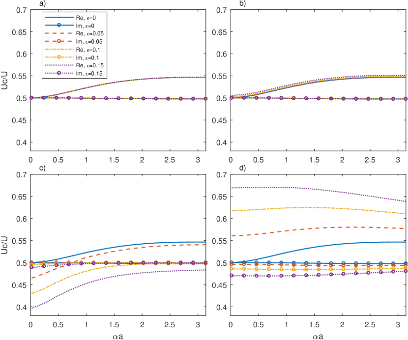
Figure 11: The convection velocity and growth rate of the mode $-2$ jet instability waves for vortex sheets of different lobed geometry: a) $N=1$; b) $N=2$; c) $N=3$; d) $N=5$.

In summary, the stability characteristics of base flows of a lobed vortex-sheet type are different from those of axisymmetric ones. The differences consist of changes to both the convection velocity and the temporal growth rate of instability waves. The changes become more pronounced as the number of lobes $N$ and the penetration ratio $\epsilon$ increase. However, instability waves with different mode numbers are affected differently by the lobed geometry. In particular, little change occurs for mode $0$, no matter how large both $N$ and $\epsilon$ are. On the other hand, an evident alteration of the characteristics of jet instability waves with large mode numbers occurs when $N>1$. For $N=3$ and $N=5$, azimuthally even and odd instability waves demonstrate the same characteristics. However, for $N=2$ and $N=1$, even and odd instability waves of lobed jets exhibit two different types of behaviour, with one having favourable effects on installed jet noise reduction and the other having adverse. Therefore, for the sake of suppressing instability waves, or achieving installed jet noise reduction, it is desired to use a lobed profile of large $N$, such as $N=5$, with a large penetration ratio. Because this results in a larger reduction of the temporal growth rates, and hence may lead to weaker instability waves.

Note that the results discussed above are obtained from a temporal analysis, from which the results of a spatial analysis may be recovered from Gaster’s transformation (Gaster, 1962). Gaster’s transformation provides a straightforward way to connect the temporal and spatial stability analyses. One of the key assumptions used in Gaster’s transformation is that both the spatial and temporal growth rates have to be small, and under this assumption Gaster showed that, to the first-order accuracy, the temporal angular frequency, $\Re(\omega)$, rather than the convection velocity $\Re(\omega)/\alpha$, is the same as the spatial angular frequency, and the temporal growth rate is equal to the product of the spatial growth rate and the temporal group velocity. With the temporal results available, we can therefore obtain the spatial growth rate by using Gaster’s transformation, provided the aforementioned assumption is not violated. Care must be taken for the spatial convection velocity as the $\Re(\omega)$ being identical does not imply the same thing for $\Re(\omega)/\Re(\alpha)$ (see the spatial convection velocity of a round vortex sheet given by Michalke (1970) for example), in which case high-order terms need to be incorporated to improve accuracy.

However, the aim of this study is to investigate the effects of lobes on the growth rates of jet instability waves so as to examine the feasibility of controlling installed jet noise using lobed jets, and these effects are unlikely to be significantly different between the temporal or spatial frameworks. For example, if the lobed geometry slightly reduces the temporal growth rate, we would expect similar behavior for the spatial growth rate. Therefore, in this paper, we focus on the temporal results only. Also note that previous studies mainly focused on chevron jets, and we do not expect their results to be identical to the stability results for the special type of lobed base flow used in this study.

4.4 The change to mode shapes

We have studied the effects of lobed geometries on the convection velocity and temporal growth rate of jet instability waves. In this section, we show their effects on the mode shapes. In the rest of this section, we present the contour plot of the pressure field corresponding to each eigen-mode. The pressure is normalized such that it is equal to the right hand side of equation 48b inside the vortex sheet. We choose to shown the pressure fields for modes $0$, $-1$ and $2$, respectively. When doing so, we fix $\epsilon=0.15$ but let $N$ vary between $1$, $2$, $3$ and $5$, respectively. For each mode at each value of $N$, we show the pressure distribution at a low frequency $\alpha a\approx 0.25$ and then at a high frequency $\alpha a\approx 2.5$. These results are shown from figures 12 to 17. In each figure, the lobed profile is represented by a thick solid black line.

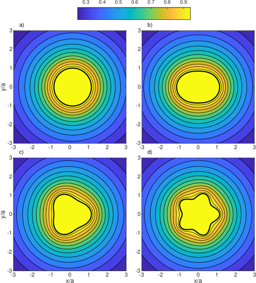
Figure 12: The shapes of mode 0 for some strongly lobed geometries when $\epsilon=0.15$ at a low frequency of $\alpha a\approx 0.25$: a) $N=1$; b) $N=2$; c) $N=3$; d) $N=5$. The thick black solid lines show the lobed vortex sheets.

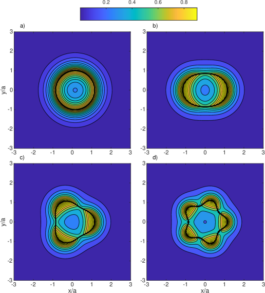
Figure 13: The shapes of mode 0 for some strongly lobed geometries when $\epsilon=0.15$ at a high frequency of $\alpha a\approx 2.5$: a) $N=1$; b) $N=2$; c) $N=3$; d) $N=5$. The thick black solid lines show the lobed vortex sheets.

Figure 12 shows the pressure distributions for mode $0$ at $\alpha a\approx 0.25$. Figure 12(a) is for $N=1$. We have mentioned that when $N=1$ the lobed profile is more or less the same as a displaced circle, and hence its stability characteristics should be nearly the same as a round jet. Figure 12(a) proves this by showing a nearly axisymmetric pressure distribution. The pressure inside the vortex sheet is nearly uniform. This is because the frequency is very low and the modified Bessel function of the first kind approaches to a constant value for a small argument. The pressure outside gradually decays to zero as the distance to the centre of the vortex sheet increases. Note how the pressure is matched continuously across the vortex sheet — another indication for a well-converged eigen-solution. Figure 12(b) shows the result for $N=2$. In this case the lobed profile resembles an ellipse. The effect of the geometry change is to stretch the pressure field inside the vortex sheet to have a distribution similar to the shape of the vortex sheet itself. The pressure outside gradually becomes axisymmetric and decays to zero at a large distance. The behaviours for $N=3$ and $5$, as shown in figures 12(c) and 12(d), respectively, are very similar to $N=2$.

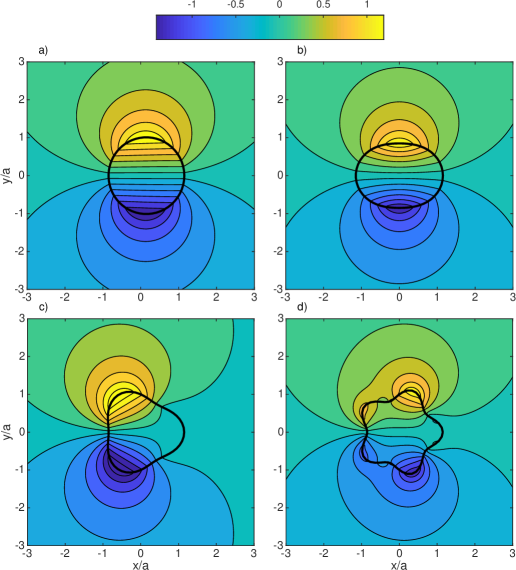
Figure 14: The shapes of mode -1 for some strongly lobed geometries when $\epsilon=0.15$ at a low frequency of $\alpha a\approx 0.25$: a) $N=1$; b) $N=2$; c) $N=3$; d) $N=5$. The thick black solid lines show the lobed vortex sheets.

Figure 13 shows the pressure fields for mode $0$ at a high frequency $\alpha a\approx 2.5$. A striking difference is the much smaller size of contour regions in each sub-figure. This is due to the fact that the pressure decays more quickly outside the vortex sheet at high frequencies. This is in accord with the fact that installed jet noise is only significant at low frequencies. Figure 13(a) again shows the result for $N=1$. One difference from figure 12(a) is that the pressure variation inside the vortex sheet is clear at this high frequency, which is what we would expect. When $N=2$, the lobed geometry has the same stretching effects as those shown in figure 12(b), but with a more marked pressure variation. The same tendencies can be seen from figures 12(c) and 12(d). The relatively insignificant change to the shape of the mode $0$ instability wave, as shown in figures 12 and 13, is consistent with the fact that both the convection velocity and temporal growth rate remain roughly the same as those for an axisymmetric jet.

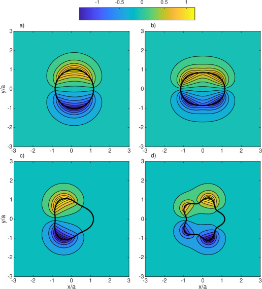
Figure 15: The shapes of mode -1 for some strongly lobed geometries when $\epsilon=0.15$ at a high frequency of $\alpha a\approx 2.5$: a) $N=1$; b) $N=2$; c) $N=3$; d) $N=5$. The thick black solid lines show the lobed vortex sheets.

Figures 14 shows the results for mode $-1$ at $\alpha a\approx 0.25$. From section 3.2, we know that for negative mode numbers the pressure distribution is antisymmetric with respect to $\phi=0$. This is reflected in figure 14. Figure 14(a) very much resembles to that of an axisymmetric jet. When $N=2$, the pressure field still largely resembles to figure 14(a). A clear change in mode shape occurs when $N=3$, as shown in figure 14(c). We can see that a three-lobe profile causes the two lobes of the pressure field to tilt towards two lobes of the vortex sheet. This signifies a potentially large change in the convection velocity and temporal growth rate. The mode shape at $N=5$ shows similar characteristics to that at $N=3$. Moreover, there are some small and locale changes in response to the appearance of local geometry corrugations. We like to point out, however, that although changes are observed, the mode shapes are still bearing the signature of conventional $\sin\phi$ behaviour, suggesting the appropriateness of our earlier mode labelling strategy.

Figure 15 is similar to figure 14 in almost every aspect, apart from the smaller size of the contour regions due to the quicker decay of the instability waves outside the vortex sheet at high frequencies. We therefore omit a repetitive description. Instead, we try to understand the behaviour of non-identical eigenvalues, as discussed in section 4.3, from the perspective of mode shapes.

We have observed that for $N=1$ and $N=2$, the eigenvalue $\lambda_{-1}$ is not degenerate any more, and consequently, only standing modes are allowed, whereas travelling modes (in the azimuthal direction, similar to a behaviour of $e^{\mathrm{i}(m\phi-\omega t)}$) are allowed for $N=3$ and $5$. To understand the difference we can compare figures 15(b) and 15(c). We conclude that, if an eigenvalue is not degenerate, then each of the symmetric plane of the lobe profile must also be a symmetric (or antisymmetric) plane of the eigen-mode. For example, in figure 15(b), the lobed profile has two symmetric planes, namely the horizontal and vertical planes, each of which is also a symmetric or antisymmetric plane of the pressure field. This is consistent with the fact that $\lambda_{1}$ is not degenerate. On the other hand, in figure 15(c), the lobed profile has three symmetric planes, but only one of them is the antisymmetric plane of the pressure field. Hence, $\lambda_{-1}$ must be degenerate. Figure 15(d) is very similar to figure 15(c). For an axisymmetric jet, the vortex sheet profile has infinitely many symmetric planes, however only two of them are the symmetric and antisymmetric planes of mode $-1$ pressure field. Therefore $\lambda_{-1}$ is degenerate for a round jet. Note that the vortex sheet profile in figure 15(a) is close to a displaced circle, but is not strictly one. It has a slight eccentricity and therefore has a non-degenerate eigenvalue.

The connection between the degeneracy and the mode shape can be understood as follows. Take figure 15(c) as an example. We mentioned that only one of three symmetric planes, which are angled by $120^{\circ}$ from each other, is the antisymmetric plane of the pressure field. Now we can rotate the pressure field by $120^{\circ}$, then the resulting pressure field must also be an eigen-solution of the stability problem, with the same eigenvalue. Therefore, the corresponding eigenvalue must be degenerate. The combination of the eigenvectors corresponding to the same eigenvalue creates infinitely many eigen-solutions, and two of them are those obtained by rotating figure 15(c) by $120^{\circ}$ and $240^{\circ}$, respectively.

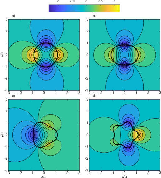
Figure 16: The shapes of mode 2 for some strongly lobed geometries when $\epsilon=0.15$ at a low frequency of $\alpha a\approx 0.25$: a) $N=1$; b) $N=2$; c) $N=3$; d) $N=5$. The thick black solid lines show the lobed vortex sheets.

We expect that the non-degeneracy is likely to occur when the mode number $n$ is equal to $\pm N/2$, $\pm N$ etc. This is because, for mode $n$, the pressure field normally has $2|n|$ lobes, and the symmetric and antisymmetric planes of such a mode can be aligned with all the symmetric planes of the vortex sheet profile. Comparing with the figures shown in section 4.3, we find that this is indeed the case. For example, we see $\lambda_{-1}\neq\lambda_{1}$ when $N=2$ and $\lambda_{-2}\neq\lambda_{2}$ when $N=2$.

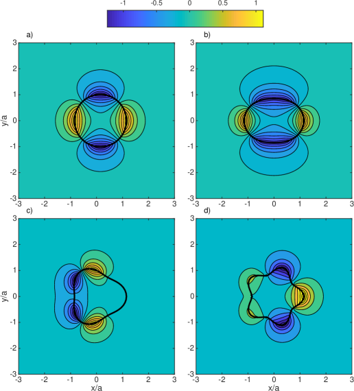
Figure 17: The shapes of mode 2 for some strongly lobed geometries when $\epsilon=0.15$ at a high frequency of $\alpha a\approx 2.5$: a) $N=1$; b) $N=2$; c) $N=3$; d) $N=5$. The thick black solid lines show the lobed vortex sheets.

Figure 16 shows the distributions of the pressure field for mode $2$ at the low frequency $\alpha a\approx 0.25$. Figure 16(a) shows its similarity to that for an axisymmetric vortex sheet while figure 16(b) for an elliptic vortex sheet. Note how the earlier conclusion about non-degeneracy remains valid in figure 16(b-d). Figure 17 shows qualitatively similar results at a higher frequency so we avoid an unnecessary repetition.

5 Conclusion

In the hope of suppressing installed jet noise, an analytical study of the stability characteristics of lobed jets of a vortex sheet type is performed. It is shown that the lobed geometry changes both the convection velocity and the temporal growth rate of the instability waves. The effects are more pronounced as the number of lobes $N$ and the penetration ratio $\epsilon$ increase. However, instability waves of different mode numbers are affected differently by the lobes. For instance, the mode $0$ is particularly insensitive to the geometry changes. Higher modes are more likely to be changed significantly when both $N$ and $\epsilon$ are sufficiently large. An interesting finding is that when $N=1$ and $N=2$ different behaviour occurs between the even and odd instability waves of certain orders, i.e. the corresponding eigenvalue becomes non-degenerate. We show that a necessary condition for a non-degenerate eigenvalue to exist is that each symmetric plane of the lobed vortex sheet must also be a symmetric or antisymmetric plane of the corresponding mode shape. This is likely to occur when the mode number $n$ is $\pm N/2$, $\pm N$ and so on. It is concluded that in order to suppress instability waves for the sake of reducing installed jet noise, a large $N$, such as $N=5$, and a large $\epsilon$ are desirable.

The insensitiveness of the mode $0$ instability waves to the lobed geometry implies that using lobed geometry hardly helps in reducing the installed jet noise due to the scattering of the mode $0$ jet instability waves. The reduction of the total installed jet noise would be somewhat limited. If the modes $0$ and $1$ (including both modes $+1$ and $-1$) instability waves are of equal strength, one would expect an observable sound reduction up to $3$ dB (in the ideal case). It is, however, worth noting that the current analysis is based on a parallel vortex sheet assumption. In realistic jets, the jet mean flow is expected to gradually become axisymmetric downstream the jet exit due to strong jet mixing. To what extent this smoothing of the lobed geometry would affect the jet stability, hence installed jet noise, requires further examination. This constitutes part of our future work.

Appendix A The kinematic and dynamic boundary conditions

The two equations shown in equation 24, together with the kinematic and dynamic boundary conditions on the vortex sheet, need to be combined to obtain the dispersion relation. The kinematic and dynamic boundary conditions can be obtained as follows. As defined above, the vortex sheet profile is given by $\mathcal{F}(\sigma,\phi)=\sigma-\mathcal{R}(\phi)=0$. One can assume that the perturbed profile can be described by the function

$$\mathcal{F}_{p}(\sigma,\phi,z,t)=\mathcal{F}(\sigma,\phi)-\eta^{\prime}(\phi,z,t)=0,$$ (49)

where $\eta^{\prime}(\phi,z,t)$ denotes a small-amplitude perturbation of the radius of the vortex-sheet profile. The kinematic boundary condition states that, on the perturbed vortex sheet,

$$\frac{\mathrm{D}\mathcal{F}_{p}(\sigma,\phi,z,t)}{\mathrm{D}t}=0.$$ (50)

Substituting the velocity on both sides of the vortex sheet to equation 50 and linearising around the unperturbed vortex sheet yields

$$\begin{dcases}\frac{\partial\eta^{\prime}}{\partial t}+U\frac{\partial\eta^{\prime}}{\partial z}-\nabla{\psi}^{-}\cdot\nabla\mathcal{F}=0,\\ \frac{\partial\eta^{\prime}}{\partial t}-\nabla{\psi}^{+}\cdot\nabla\mathcal{F}=0.\end{dcases}$$ (51)

After invoking the harmonic time and $z$ dependence ($\mathrm{e}^{\mathrm{i}\alpha z}\mathrm{e}^{-\mathrm{i}\omega t}$) and eliminating $\eta^{\prime}$, one can show that equation 51 reduces to

$$(\omega-\alpha U)\nabla\psi^{+}\cdot\boldsymbol{n}=\omega\nabla\psi^{-}\cdot\boldsymbol{n},$$ (52)

where $\boldsymbol{n}$ denotes the unit vector perpendicular to the vortex-sheet profile, which can be readily shown to be $\nabla\mathcal{F}/|\nabla\mathcal{F}|$. The dynamic boundary condition requires pressure continuity across the vortex sheet. From the linearized momentum equation, i.e. equation 4, one can readily show that

$$p^{\prime}=-\rho\left(\frac{\partial}{\partial t}+U_{z}\frac{\partial}{\partial z}\right)\psi,$$ (53)

where $U_{z}$ can be either $U$ and $0$ depending on which side of the vortex sheet is considered. Hence substituting the velocity potentials on both sides of the vortex sheet yields that on the unperturbed vortex sheet (after linearising around the unperturbed vortex sheet)

$$\omega\psi^{+}=(\omega-\alpha U)\psi^{-},$$ (54)

Appendix B The properties on rotationally symmetric matrices

Since the eigenvector $\boldsymbol{C}^{-}$ of the matrix $\boldsymbol{A}$ fully determines the eigenfunction $E_{n}^{-}(\sigma,\phi)$, it is important to examine the properties of $\boldsymbol{A}$ and its eigenvectors. In order to do this, we need to define the rotation of any vector $\boldsymbol{C}$ as $\boldsymbol{C}^{R}$, such that

$$(\boldsymbol{C}^{R})_{n}=C_{-n},$$ (55)

where $(\boldsymbol{C}^{R})_{n}$ denotes the $n$th the element of the rotation vector $\boldsymbol{C}^{R}$ and $C_{n}$ is the $n$th element of $\boldsymbol{C}$. Note here the index of the vector $\boldsymbol{C}$ ranges from $-M$ to $M$. Similarly, we can define the rotation of any matrix $\boldsymbol{B}$ as

$$(\boldsymbol{B}^{R})_{ij}=B_{(-i)(-j)},$$ (56)

where $(\boldsymbol{B}^{R})_{ij}$ denotes the element of $\boldsymbol{B}^{R}$ at the $i$th row and the $j$th column, and $B_{ij}$ are the indexed elements of matrix $\boldsymbol{B}$. If a vector $\boldsymbol{C}$ is equal to its rotation, we define it as symmetric. If, on the other hand, $\boldsymbol{C}=-\boldsymbol{C}^{R}$, we define it as antisymmetric. Similarly, if a matrix $\boldsymbol{B}$ is equal to its rotation, we define it as rotationally symmetric. Anti-rotational symmetry follows a self-explanatory definition. One can now show that $(\boldsymbol{BC})^{R}=\boldsymbol{B}^{R}\boldsymbol{C}^{R}$, because

$$\big{(}(\boldsymbol{B}\boldsymbol{C})^{R}\big{)}_{i}=\sum_{j=-M}^{M}B_{(-i)j}C_{j}=\sum_{j=-M}^{M}B_{(-i)(-j)}C_{-j}=\big{(}\boldsymbol{B}^{R}\boldsymbol{C}^{R}\big{)}_{i},$$ (57)

where $i$ can be any number between $-M$ to $M$. Replacing the vector $\boldsymbol{C}$ in the above equations with a matrix $\boldsymbol{B}_{2}$ does not invalidate the formula, i.e. $(\boldsymbol{BB}_{2})^{R}=\boldsymbol{B}^{R}\boldsymbol{B}_{2}^{R}$ also holds. Therefore, if both $\boldsymbol{B}$ and $\boldsymbol{B}_{2}$ are rationally symmetric matrices, then the product of them is also rotationally symmetric. This is because

$$(\boldsymbol{BB}_{2})^{R}=\boldsymbol{B}^{R}\boldsymbol{B}_{2}^{R}=\boldsymbol{BB}_{2}.$$ (58)

We now prove that the inverse of a rotationally symmetric matrix, if exists, is also rotationally symmetric. First, because it is assumed that the inverse of the rotationally symmetric $\boldsymbol{B}$ exists, we denote its column vectors by $\boldsymbol{D}_{i}$ ($i=-M\dots M$), i.e.

$$\boldsymbol{B}^{-1}=[\boldsymbol{D}_{-M}\dots\boldsymbol{D}_{0}\dots\boldsymbol{D}_{M}].$$ (59)

Then according to the definition of the inverse matrix, one has

$$[\boldsymbol{B}\boldsymbol{D}_{-M}\dots\boldsymbol{B}\boldsymbol{D}_{0}\dots\boldsymbol{B}\boldsymbol{D}_{M}]=[\boldsymbol{I}_{-M}\dots\boldsymbol{I}_{0}\dots\boldsymbol{I}_{M}],$$ (60)

where $\boldsymbol{I}_{i}$ is the $i$th column of the identity matrix. Now for any positive number $i$, one has

$$\boldsymbol{B}\boldsymbol{D}_{i}=\boldsymbol{I}_{i}.$$ (61)

If taking the rotation of both sides of equation 61, one obtains

$$\boldsymbol{B}\boldsymbol{D}_{i}^{R}=\boldsymbol{I}_{-i},$$ (62)

where use is made of the fact that $\boldsymbol{I}_{i}^{R}=\boldsymbol{I}_{-i}$ and $\boldsymbol{B}$ is equal to its own rotation. Comparing equation 62 with the $-i$ column of equation 60, we have $\boldsymbol{D}_{i}^{R}=\boldsymbol{D}_{-i}$. This is because $\boldsymbol{B}$ is invertible, its has a full rank and the solution of equation 62 is unique. We have now proved that $\boldsymbol{B}^{-}$ is indeed a rationally symmetric matrix.

Examining the definitions of all the relevant $\boldsymbol{I}$ and $\boldsymbol{K}$ matrices, it is trivial to show that they are all rotationally symmetric. Based on the two conclusions discussed above, because the matrix $\boldsymbol{A}$ can be written as

$$\boldsymbol{A}=\widetilde{\boldsymbol{I}}_{k}^{-1}\widetilde{\boldsymbol{K}}_{k}\widetilde{\boldsymbol{K}}_{d}^{-1}\widetilde{\boldsymbol{I}}_{d},$$

it can be easily shown that $\boldsymbol{A}$ is rotationally symmetric. One important property that follows is that if a vector $\boldsymbol{C}^{-}$ is one of the eigenvectors of $\boldsymbol{A}$, so is $\boldsymbol{C}^{-R}$. This follows naturally after taking the rotation of both sides of the eigenvalue equation $\boldsymbol{A}\boldsymbol{C}^{-}=\lambda\boldsymbol{C}^{-}$. One consequence of this property is that if an eigenvalue $\lambda_{n}$ of matrix $\boldsymbol{A}$ has no multiplicity, its eigenvector $\boldsymbol{C}^{-}$ must be either symmetric or antisymmetric. The second important property is that, for each multiple-folded eigenvalue $\lambda_{n}$, we can always construct both a symmetric (e.g. $\boldsymbol{C}^{-}+\boldsymbol{C}^{-R}$) and an antisymmetric (e.g. $\boldsymbol{C}^{-}-\boldsymbol{C}^{-R}$) eigenvector. These properties are essential when we try to assign an order to each obtained eigenvector in Appendix C.

Appendix C The mode labelling strategy

It is not difficult to show that, when $\epsilon=0$, $\boldsymbol{A}$ is diagonal and its eigenvalues (diagonal elements) are

$$\lambda_{n}=\frac{K_{n}^{\prime}(\alpha a)I_{n}(\alpha a)}{K_{n}(\alpha a)I_{n}^{\prime}(\alpha a)}$$ (63)

and their corresponding normalized eigenvectors are

$$\boldsymbol{C}^{-}=\left[\ldots,0,\ldots,0,\ldots,1,\ldots\right]^{T},$$ (64)

where $1$ appears at the position of $C_{n}^{-}$. The well-known results for the cylindrical vortex-sheet flow are recovered. When $\epsilon$ increases gradually, we expect that the eigenvector gradually changes to

$$\boldsymbol{C}^{-}=\left[\ldots,a_{-n},\ldots,a_{0},\ldots,1-a_{n},\ldots\right]^{T},$$ (65)

where $a_{n}$ are complex numbers and $|a_{n}|\ll 1$. We may use this dominant-component property of $\boldsymbol{C}^{-}$ to label the order of the eigenfunctions. That is, the eigenfunction determined by the eigenvector

$$\boldsymbol{C}^{-}=\left[\ldots,C_{-n}^{-},\ldots,C_{0}^{-},\ldots,C_{n}^{-},\ldots\right]^{T}$$ (66)

has an mode number $n$, if

$$||\boldsymbol{C}^{-}-\boldsymbol{G}||=\sqrt{\sum_{j=-M}^{M}(|C_{j}^{-}|-G_{j})^{2}}$$ (67)

yields a minimum value when

$$\boldsymbol{G}=\left[\ldots,0,\ldots,0,\ldots,g_{n}=1,\ldots\right]^{T},$$ (68)

where $g_{n}$ is the element of the vector $\boldsymbol{G}$.

This strategy, however, hinges on the assumption that there is only one dominant component in the eigenvector $\boldsymbol{C}^{-}$. However, this is not always possible. For example, when $\epsilon\neq 0$, $\lambda_{n}$ and $\lambda_{-n}$ do not necessarily have to be same any more. As we discussed above, the eigenvector must be either symmetric or antisymmetric. Since both symmetric and antisymmetric eigenvectors have two dominant components at $n$ and $-n$ respectively ($\lambda_{n}\neq\lambda_{-n}$, therefore one cannot perform a linear combination of the two corresponding eigenvectors), it is hard to determine whether this mode should be called mode $n$ or $-n$.

To overcome this problem, we force each eigenvector to be either symmetric or antisymmetric. This is always possible, because, as we proved earlier, the eigenvector $\boldsymbol{C}^{-}$ must be either symmetric or antisymmetric if $\lambda_{n}\neq\lambda_{-n}$. And if $\lambda_{n}=\lambda_{-n}(n>0)$, we can always make use the second property of the eigenvectors and redefine one of the two corresponding eigenvectors to be symmetric and the other antisymmetric. In doing so, no matter whether $\lambda_{n}$ and $\lambda_{-n}$ are equal or not, each eigenvector would have two dominant components. Now for the symmetric eignvectors if $||\boldsymbol{C}^{-}-\boldsymbol{G}||$ obtains its minimum when

$$\boldsymbol{G}=\left[\ldots,g_{-n}=\sqrt{2}/2,\ldots,0,\ldots,g_{n}=\sqrt{2}/2,\ldots\right]^{T},$$ (69)

we label the eigenvector as mode $n$. For anti-symmetric eigenvectors we label it as $-n$ in a similar manner. For $n=0$, it is trivial to label its mode number, and because we require $C_{0}^{-}\neq 0$, it can be shown that the eigenvector must be symmetric. By labelling the eigenvectors in this way, from equation 43, this means that all nonnegative eigenfunctions are even functions of $\phi$ and negative ones odd.

References

- Batchelor & Gill (1962) Batchelor, G. K. & Gill, A. E. 1962 Analysis of the stability of axisymmetric jets. Journal of Fluid Mechanics 14, 529–551.
- Baty & Morris (1995) Baty, R. S. & Morris, P. J. 1995 The instability of jets of arbitrary exit geometry. International Journal for Numerical Methods in Fluids 21 (9), 763–780.
- Cavalieri et al. (2014) Cavalieri, A. V. G., Jordan, P., Wolf, W. & Gervais, Y. 2014 Scattering of wavepackets by a flat plate in the vicinity of a turbulent jet. Journal of Sound and Vibration 333, 6516–6531.
- Cavalieri et al. (2013) Cavalieri, A. V. G., Rodríguez, D., Jordan, P., Colonius, T. & Gervais, Y. 2013 Wavepackets in the velocity field of turbulent jets. Journal of Fluid Mechanics 730, 559–592.
- Crighton (1973) Crighton, D. G. 1973 Instability of an elliptic jet. Journal of Fluid Mechanics 59 (4), 665–672.
- Gaster (1962) Gaster, M. 1962 A note on the relation between temporally-increasing and spatially-increasing disturbances in hydrodynamic stability. Journal of Fluid Mechanics 14, 222–224.
- Hu et al. (2002) Hu, H., Saga, T., Kobayashi, T. & Taniguchi, N. 2002 Mixing process in a lobed jet flow. AIAA Journal 40 (7).
- Kawahara et al. (2003) Kawahara, G., Jiménez, J., Uhlmann, M. & Pinelli, A. 2003 Linear instability of a corrugated vortex sheet - a model for streak instability. Journal of Fluid Mechanics 483, 315–342.
- Kopiev et al. (2004) Kopiev, V. F., Ostrikov, N. N., Chernyshev, S. A. & Elliot, J. W. 2004 Aeroacoustics of supersonic jet issued from corrugated nozzle: new approach and prospects. International Journal of Aeroacoustics 3 (3), 199–228.
- Lajús Jr. et al. (2015) Lajús Jr., F. C., Cavalieri, A. V. G. & Deschamps, C. J. 2015 Spatial stability characteristics of non-circular jets. In Proceedings of 21st AIAA/CEAS Aeroacoustics Conference. American Institute of Aeronautics and Astronautics, 2015-2537.
- Li et al. (2001) Li, H., Hu, H., Kobayashi, T., Saga, T. & Taniguchi, N. 2001 Visualization of multi-scale turbulent structure in lobed mixing jet using wavelets. Journal of Visulization 4 (3), 231–238.
- Li et al. (2002) Li, Hui, Hu, Hui, Kobayashi, Toshio, Saga, Tetsuo & Taniguchi, Nobuyuki 2002 Wavelet multiresolution analysis of stereoscopic particle-image-velocimetry measurements in lobed jet. AIAA Journal 40 (6).
- Lyu et al. (2017) Lyu, B., Dowling, A. & Naqavi, I. 2017 Prediction of installed jet noise. Journal of Fluid Mechanics 811, 234–268.
- Lyu & Dowling (2016) Lyu, B. & Dowling, A. P. 2016 Noise prediction for installed jets. In Proceedings of 22nd AIAA/CEAS Aeroacoustics Conference. American Institute of Aeronautics and Astronautics, aIAA 2016-2986.
- Mankbadi & Liu (1984) Mankbadi, R. & Liu, J. T. C. 1984 Sound generated aerodynamically revisited: large-scale structures in a turbulent jet as a source of sound. Philosophical Transactions of the Royal Society of London A 311 (1516), 183–217.
- Miao et al. (2015) Miao, T., Dmitriy, L., Liu, J., Qin, S., Wu, D., Chu, N. & Wang, L. 2015 Study on the flow and acoustic characteristics of submerged exhaust through a lobed nozzle. Acoustics Australia 43, 283–293.
- Michalke (1970) Michalke, A. 1970 A wave model for sound generation in circular jets. Technical report Deutsche Luftund Raumfahrt.
- Morris (1988) Morris, P. J. 1988 Instability of elliptic jets. AIAA Journal 26 (2), 172–178.
- Morris (2010) Morris, P. J. 2010 The instability of high speed jets. International Journal of Aeroacoustics 9 (1-2), 1–50.
- Piantanida et al. (2016) Piantanida, S., Jaunet, V., Huber, J., Wolf, W.R., Jordan, P. & Cavalieri, A.V.G. 2016 Scattering of turbulent-jet wavepackets by a swept trailing edge. Journal of the Acoustical Society of America 140 (6), 4350–4359, cited By 2.
- Sinha et al. (2016) Sinha, A., Gudmundsson, K., Xia, H. & Colonius, T. 2016 Parabolized stability analysis of jets from serrated nozzles. Journal of Fluid Mechanics 789, 36–63.
- Tam & Thies (1993) Tam, C. K. W. & Thies, A. T. 1993 Instability of rectangular jets. Journal of Fluid Mechanics 248, 425–448.
- Tam & Zaman (2000) Tam, C. K. W. & Zaman, K. B. M. Q. 2000 Subsonic jet noise from nonaxisymmetric and tabbed nozzles. AIAA Journal 38 (4), 592–599.
- Tinney & Jordan (2008) Tinney, C. E. & Jordan, P. 2008 The near pressure field of co-axial subsonic jets. Journal of Fluid Mechanics 611, 175–204.
- Zaman et al. (2003) Zaman, K. B. M. Q., Wang, F. Y. & Georgiadis, N. J. 2003 Noise, turbulence and thrust of subsonic free jets from lobed nozzles. AIAA Journal 41 (3), 389–407.