Recent developments in radioactive charged-particle emissions and related phenomena

Abstract

The advent and intensive use of new detector technologies as well as radioactive ion beam facilities have opened up possibilities to investigate alpha, proton and cluster decays of highly unstable nuclei. This article provides a review of the current status of our understanding of clustering and the corresponding radioactive particle decay process in atomic nuclei. We put alpha decay in the context of charged-particle emissions which also include one- and two-proton emissions as well as heavy cluster decay. The experimental as well as the theoretical advances achieved recently in these fields are presented. Emphasis is given to the recent discoveries of charged-particle decays from proton-rich nuclei around the proton drip line. Those decay measurements have shown to provide an important probe for studying the structure of the nuclei involved. Developments on the theoretical side in nuclear many-body theories and supercomputing facilities have also made substantial progress, enabling one to study the nuclear clusterization and decays within a microscopic and consistent framework. We report on properties induced by the nuclear interaction acting in the nuclear medium, like the pairing interaction, which have been uncovered by studying the microscopic structure of clusters. The competition between cluster formations as compared to the corresponding alpha-particle formation are included. In the review we also describe the search for super-heavy nuclei connected by chains of alpha and other radioactive particle decays.

1 Introduction

The process leading to the emission of alpha-particles from nuclei is a subject that has been studied since the beginning of modern physics at the end of the 19th Century [1, 2]. However nearly three decades had to pass before Gamow could explain how an alpha-particle can overcome the Coulomb and centrifugal barriers that trap it inside the nucleus [3]. That was a great breakthrough which can be viewed as a cornerstone of the probabilistic interpretation of quantum mechanics. Gamow explained the decay as the penetration of an already formed alpha particle through the Coulomb and centrifugal barriers. To obtain the proper units, Gamow also introduced the concept of “assault frequency” which is an effective quantity that, due to the Pauli principle, does not carry any quantum mechanics validity. This theory has been extremely successful in explaining relative decay widths, but could not describe absolute decay widths. Yet the calculation of the penetrability is relatively easy and therefore the theory was applied in many situations, trying to get the absolute decay widths by adjusting effective parameters, such as the assault frequency, to fit the corresponding decay width. These effective theories are very useful because they are easy to apply. However, a proper calculation of the decay process needs to address the clustering of the nucleons on the surface of the mother nucleus and the following penetrability of the cluster thus formed through the Coulomb and centrifugal barriers. The evaluation of the cluster formation probability is a challenging undertaking because a proper description of the cluster in terms of its components requires a microscopic framework that is highly complex. This is the reason why effective approaches are used when dealing with clusterization.

Yet, one has to surmise the lack of a firm theoretical foundation for the effective quantities thus introduced. This would require a microscopic treatment of the decay process which includes the degrees of freedom of all nucleons involved in the decay. Microscopic theories are not always famous for their plausibility or accurate predictions. Phenomenological approaches often surpass them in both respects by their simplicity and aptitude, owing largely to their tendency to wrap unknown aspects and even inconsistent ingredients into adjustable parameters. One may wonder how can effective theories, in spite of their obvious shortcomings, be so successful in describing alpha decay. This is due to the efforts of many researches through years of adjustments to new experimental data which resulted in methods or, perhaps more proper, effective formulae which reproduce reasonable well alpha-decay data. In really fundamental microscopic theories, on the contrary, no ad hoc assumptions must be invoked, and the number of free parameters is to be reduced to a minimum, preferably to none. One cannot really understand the underlying mechanism of decay processes without describing them by parameter-free microscopic theories, free of ad hoc elements. To approach this ideal, one has to use dynamical theories in which the states involved are constructed by some (approximate) solution of a model Schrödinger equation.

The study of particle radioactivity have been a primordial interest in nuclear physics. These developments are going on even at present. In this review we will present developments that took place through the many years. Indeed, nuclear physics is undergoing a renaissance from both experimental and theoretical physics point of views with the availability of intense radioactive ion beams and new detecting and supercomputing technologies. The new nuclear facilities have opened up possibilities to investigate highly unstable nuclei. One of the most important aspects in these searches is the possibility of discovering so far unknown superheavy nuclei. Here alpha emission is one of the dominant forms of decay. This decay occurs most often in massive nuclei that have relatively large proton to neutron ratios, where it can reduce the ratio of protons to neutrons in the parent nucleus, bringing it to a more stable configuration in the daughter nucleus. Almost all observed proton-rich or neutron-deficient nuclei starting from mass number $A\sim 150$ decay through alpha-emission channels, as shown in Fig. 1 where we plotted the observed ground state decay modes for nuclei with $Z\geq 50$. The emission of heavy clusters, which is also observed in heavy nuclei, is closely related to spontaneous fission [4, 5, 6]. In fact fission and $\alpha$ emission may compete with similar probabilities as decay modes in heavy and superheavy nuclei.

Besides the decay of clusters from nuclei, we will also report studies on proton and two-proton radioactivity. We use the term “proton radioactivity” to describe the process leading to the decay of a nucleus by emitting a proton. It may seem more natural to call this process “proton decay”, as one calls “alpha decay” the emission of an alpha particle from a nucleus. The problem with the name ”proton decay” is that it may be confused with the hypothetical decay of a proton into lighter particles, such as a neutral pion and a positron. There is no evidence at present that proton decay in this sense exists. In this review we will use indiscriminately the terms “proton radioactivity”, “proton emission” and “proton decay” to describe the emission of a proton from a nucleus. The name used for the proton decay process should not be confusing here, since we refer to nuclear decay only.

Our aim in this review is to present in a clear and pedagogical fashion the most relevant investigations that have been performed during the last couple of decades by outstanding researches in unveiling the difficult but thrilling subject of radioactive particle decay from nuclei. This includes, besides $\alpha$-decay, proton-, two-proton- and heavy-cluster emission, as have been outlined above.

Figure 1: Ground-state decay modes of nuclei with proton number $Z\geq 50$ extracted from Nubase2016 [7] which includes $\alpha$ decay (yellow), $\beta^{+}$ (red), $\beta^{-}$ (green), electron capture (dark orange), fission (green). The more rare cases of proton decays and cluster decays are marked with dark blue and purple colors, respectively. We use triangles to indicate secondary decay modes. The solid lines correspond to the proton shell closures $Z=50$, 82 and neutron shell-closures $N=50$, 82 and 126.

2 General formalism

In this Section we will briefly review theoretical results acquired before the period covered by this report. The resulting formalism is fundamental to understand the decay processes to be included here.

There is an important difference between the decays of clusters and one- and two-proton decays. In the firt case one has to consider the formation of the clusters, including alpha and heavier clusters like ¹⁴C, starting from the nucleons that constitute the decaying mother nucleus. This is an extremely complicated process which requires the knowledge of the mechanisms that induce the cluster formation as well as the description of the motion of the already formed cluster while departing from the daughter nucleus.

The calculation of the decay of the lightest cluster that happens in Nature, that is alpha-decay, is already a difficult undertaking which induced much debate and arguments through the years. A number of theories were proposed which are by now nearly forgotten. For a review on this one can see Ref. [8]. The microscopic treatment of alpha decay required a general framework which was provided by the introduction of the R-matrix theory as formulated by Teichman and Wigner [9]. In this formalism the collision between two nuclei leading to a compound system and its subsequent decay is described by dividing the configuration space of the composite system into an “internal region”, to which the compound state is restricted, and the complementary “external region”. This division is made such that in the external region only the Coulomb interaction is important and the system in the outgoing channel behaves like a two-particle system. This is exactly what occurs in alpha decay, where the outgoing channel consists of two fragments, the alpha particle and the daughter nucleus, interacting through the Coulomb interaction only. The important feature of the formalism is that the residues of the R-matrix is proportional to the decay width of the resonance induced by the decay process. This formalism was applied by Thomas to evaluate the $\alpha$-decay width in a profound but difficult paper [10]. A more accessible derivation of the Thomas expression for the width can be found in Ref. [11].

Thomas classical expression has the form

$$\Gamma_{c}(R)=\hbar/T=\frac{\hbar^{2}k}{\mu}\frac{R^{2}|{\cal F}_{c}(R)|^{2}}{F^{2}_{c}(R)+G^{2}_{c}(R)}$$ (1)

where $c$ labels the decaying channel, $k$ is the linear momentum carried by the $\alpha$-particle, $\mu$ is the reduced mass, $R$ is the distance between the mass centres of the daughter and cluster nuclei, $F_{c}(R)$ ($G_{c}(R)$) is the regular (irregular) Coulomb function corresponding to the two-body system in the outgoing channel and ${\cal F}_{c}(R)$ is the formation amplitude, i. e. the wave function of the mother nucleus at the point R. It is very important to underline that the distance $R$ in Eq. (1) corresponds to the matching distance where the internal and external wave functions coincide.

The way Thomas wrote the width, which, as in Eq. (1), may indicate that it is $R$-dependent, was the origin of much confusion. This confusion may have been strengthened by the name used for $R$, namely the “channel radius”. There have been authors claiming that since all function in Eq. (1) depend exponentially upon $R$ the width itself was strongly $R$-dependent. Therefore the formalism was useless, as indeed it would have been if such dependence existed. The point $R$ should be chosen outside the range of the nuclear central field induced by the daughter nucleus. At this point the $\alpha$-particle is already formed. Therefore the width above is independent of $R$. This property was often used in microscopic calculations to probe that the results were reliable. This was earliest done in Ref. [12].

The width (1) is valid for the decay of any cluster, not only alpha-particles (the subscript $c$ in Eq. (1 refers to ”cluster”). That equation is often written in terms of the penetrability $P_{c}(R)$, i. e. the probability that the already formed cluster penetrates the Coulomb and centrifugal barriers starting at the point $R$. It is given by [10]

$$P_{c}(R)=\frac{kR}{F^{2}_{c}(R)+G^{2}_{c}(R)}$$ (2)

and the width becomes

$$\Gamma_{c}(R)=\frac{\hbar^{2}R}{\mu}P_{c}(R)|{\cal F}_{c}(R)|^{2}.$$ (3)

The penetrability is strongly dependent upon the $Q$-value of the decay channel. It is also strongly dependent upon the distance $R$, a feature which is shared by the formation probability. When the calculation is performed properly, as mentioned above, the two $R$-dependences cancel each other and the evaluated half lives are radius independent. Effective approaches totally ignore the dependence of the formation probability upon the distance. Instead the free parameters are assumed to somehow take care of it. That is the reason why it is often stated that the penetrability is overwhelmingly dominant in the alpha decay process.

The time when Thomas presented his formula, in the 1950s, was the age of the shell model. The shell model is, more than a model, a tool that provides an excellent representation to describe nuclear dynamics. One would then think that the shell model should be capable of taking into account any correlations if the corresponding basis is large enough. This was clear to the pioneers who started to use the shell model for the description of $\alpha$-decay. It aroused optimism at the beginning that very simple shell-model calculations were able to describe the low energy spectra of nuclei [13]. Supported by this result, and due to the poor computing facilities available at that time, only one configuration was included in the first applications of the shell model to the description of the mother nucleus in $\alpha$-decay. The results were discouraging since the theoretical decay rates were significantly smaller than the corresponding experimental values by 4-5 orders of magnitude [14]. This failure arouse doubts about the validity of the shell model itself [15]. It was later found that the inclusion of more configurations in the description of the mother nucleus improved the result dramatically. This, as well as the use of the BCS formalism to describe superfluid and deformed nuclei, was an important theme during a rather long time. A detailed review of these developments can be found in Ref. [16], where even efforts performed to describe the clustering process in heavy nuclei are reviewed. The related subject of clustering in light nuclei is reviewed in e.g. Refs. [17, 18, 19, 20].

It is expected that the decays of the proton, the $\alpha$ particle and heavy clusters can be simultaneously described by a two-step mechanism, as indicted by the Thomas expression for the width, of first formation and then the penetration of the particle through a static Coulomb and centrifugal barriers. This is illustrated in Fig. 2. the charge-particle decay process can be evaluated in two steps in regions divided by the radius $R$: the inner process which describes the dynamic motion of the nucleons composing the emitting-particle inside the nucleus and the possibility for it to be formed and emitted, and the outer process which describes the penetration of the particle through the Coulomb and centrifugal barriers and are independent of nuclear structure effects. The emitting-particle formation amplitude that reflects the overlap between the parent and daughter wave functions and the intrinsic structure of the emitting particle. This scheme avoids the ambiguities of the deduced spectroscopic factor in relation to the surface effects and quantifies in a more precise manner the nuclear many-body structure effects. It is also valid for all charged particle decays. On the other hand, the spectroscopic factor is a model dependent quantity. It makes sense only if the same single-particle wave function are using in both the structure and the decay channel.

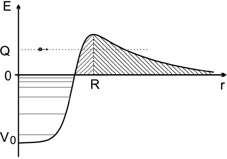
Figure 2: A one-dimensional schematic view of the particle emission process through the Coulomb barrier. Adapted from Ref. [21].

3 Proton radioactivity

We start this theoretical review of the developments in radioactive particle decay during the last couple of decades with the microscopic treatment of proton decay. Among all particle decay processes the simplest one is proton decay since in this case one avoids to deal with the most complicated feature of particle decay, namely the formation and intrinsic structure of the decaying particle. Therefore we start the discussions of the Thomas formula (1) by presenting this case, which is just fitted to understand features like e. g. the independence of the decay width upon the radius $R$. We will briefly present the formalism, for details see Ref. [11].

The proton formation amplitude in Eq. (1) has the form,

$${\cal F}_{p}(R)=\int d{\mathbf{R}}d\xi_{d}[\Psi_{d}(\xi_{d})\chi(\xi_{p})Y_{l}(\mathbf{R})]^{*}_{J_{m}M_{m}}\Psi_{m}(\xi_{d},\xi_{p},\mathbf{R}),$$ (4)

where $d$, $p$ and $m$ label the daughter, proton and mother nuclei, respectively. The variables $\xi$ label the necessary different degrees of freedom. The internal wave function of the daughter nucleus is $\Psi_{d}(\xi_{d})$. The internal proton wave function, $\chi(\xi_{p})$, is the 1/2-spinor corresponding to the emitted proton, which carries an angular momentum $l$. One does not need to consider the intrinsic structure of the emitting-proton when evaluating the formation probability.

For simplicity we will assume that the decaying (mother) nucleus is spherical and that it consists of one proton outside a double closed shell. In this simple case the mother nucleus wave function is

$$\Psi_{m}(\xi_{d},\xi_{p},\mathbf{R})=[\Psi_{d}(\xi_{d})\chi(\xi_{p})Y_{l}(\mathbf{R})]_{J_{m}M_{m}}\psi_{p}(R).$$ (5)

and, therefore, the formation amplitude ${\cal F}_{p}(R)$ is just the single-particle wave function $\psi_{p}(R)$. The index $p$ labels $(nlj)$, where $n$ is the principal quantum number and $(lj)$ the orbital and total angular momenta of the proton moving in the central field induced by the daughter nucleus.

Since the mother nucleus decays, the proton has to move in orbits lying in the continuum part of the spectrum. To be observable, however, the mother nucleus has to live a time long enough for the detector to be able to measure it. The shortest mean time $T$ that one can measure at present is of the order of $10^{-13}$ sec. That implies that the widest resonance one can measure is of the order (with $\hbar=6.6\times 10^{-22}$ Mev sec) $\Gamma=\hbar/T$=6.6$\times 10^{-9}$ MeV. This is an extremely narrow resonance and therefore the proton may be considered to be moving in a bound state. In other words one may consider that the proton wave function vanish at long distances. But for our purpose it is safer to apply the more realistic outgoing boundary condition. There are a number of computer codes that allow one to evaluate outgoing wave functions. One that has proved to be very stable is the code GAMOW [22, 23]. The outgoing boundary condition implies that the calculated energy ${\cal E}_{nlj}$ is complex, i. e. it is ${\cal E}_{nlj}=E_{nlj}-i\Gamma_{nlj}/2$, where $E_{nlj}$ is the position and $\Gamma_{nlj}$ the width of the resonance. The imaginary part (i. e.. the width) vanishes and the real part is negative for bound and antibound states. The evaluation of the wave function ${\cal F}_{nlj}(R)$ is performed by first choosing an appropriate central field, for instance a Woods-Saxon potential. The code provides all possible states, i. e. the resonances, the bound and the antibound states. For details see Ref. [22]. An alternate code has been written by one of us by using the log-derivative method.

Only the Coulomb interaction is important at distances $R$ beyond the central field. Therefore the wave function at those distances has the form

$${\cal F}^{Coul}_{nlj}(R)=N_{nlj}[G_{lj}(R)+iF_{lj}(R)]/R$$ (6)

where $N$ is a normalization constant and $F$ and $G$ are the regular and irregular Coulomb functions, respectively. The constant $N$ is determined by matching at the radius $R$ the wave function evaluated inside the nucleus, i. e. ${\cal F}_{nlj}(R)$ (Eq. (4)) to ${\cal F}^{Coul}_{nlj}(R)$. The constant $N$ becomes

$$|N_{nlj}|^{2}=R^{2}\frac{|{\cal F}_{nlj}(R)]^{2}}{F^{2}_{lj}(R)+G^{2}_{lj}(R)}$$ (7)

Since $N$ is independent upon $R$, one sees that the Thomas expression (1) is also $R$-independent. The constant $|N|^{2}$ is proportional to the width of the resonance [11].

It is not difficult to extend the formalism above to deformed nuclei. Assuming that the daughter nucleus is even-even the angular momentum projected wave function is given by

$$\Psi^{JMK}_{m}=\sqrt{\frac{\hat{J}}{16\pi^{2}}}[{\cal D}^{J}_{MK}\chi_{{}_{K}}+(-1)^{J+K}{\cal D}^{J}_{M-K}\chi_{{}_{\bar{K}}}]$$ (8)

where standard notation was used [11]. The intrinsic single-particle wave function $\chi$ can be expanded in spherical components as,

$$\chi_{K}(r)=\sum_{j\leq K}\alpha_{lj}(r)[Y_{l}(\hat{r})\chi_{1/2}]_{jK}$$ (9)

where the orbital angular momentum $l$ is determined by the parity of the state.

Decays from high lying states are not likely because electromagnetic transitions from excited states are faster than proton decay. But it has to be stressed that proton decay transitions from excited states has also been measured, for instance in Ref. [24]. For simplicity we will consider the most common case of ground state to ground state transitions. Therefore it is $J=K$. Since the daughter nucleus is even-even the corresponding quantum numbers are $J_{d}=M_{d}=K_{d}$=0. As a result the angular momentum of the outgoing proton is $j_{p}=J=K$.

As in the spherical case above, at distance $R$ beyond the deformed mean field only the Coulomb interaction is active. One thus has,

$$R\chi^{ext}_{{}_{K}}(R)=\sum_{lj}N_{lj}[G_{lj}(R)+iF_{lj}(R)][Y_{l}(\hat{r})\chi_{1/2}]_{jK}$$ (10)

and as before the set of constants $N_{lj}$ are determined by matching the external wave function $\chi^{ext}$ to the internal one, Eq. (9).

Considering the angular momentum constraints discussed above and the orthogonality of the partial waves, the partial decay width to the channel $(l_{p}j_{p})$ is

$$\Gamma_{l_{p}j_{p}}(R)=\frac{\hbar^{2}k}{\mu}\frac{R^{2}\alpha^{2}_{l_{p}j_{p}}(R)}{F^{2}_{l_{p}j_{p}}(R)+G^{2}_{l_{p}j_{o}}(R)}$$ (11)

This formalism was applied in Ref. [11] to study the proton decay from the ground state of the deformed nucleus ¹¹³Ce. It was found that proton decay is a powerful tool to probe small components of the deformed wave function which would be difficult to do with other probes.

3.1 Systematic studies of Proton radioactivity and nuclear structure

Proton emission was first observed rather recently in the context of nuclear radioactivity. This happened in 1970 when the decay of ⁵³Co from an excited high-spin isomer was measured [25, 26]. That the mother nucleus was excited is not surprising since the proton is bound to the mother nucleus in its ground state. That is, the proton $Q$-value (which is proportional to the proton kinetic energy at large distance) corresponding to the decay from ⁵³Co(gs) to the ground state of the daughter nucleus is negative. Therefore the proton can be emitted only from a state which is excited enough.

With the improvement of experimental facilities, which allowed one to investigate nuclei lying close to the proton drip line, proton emission from ground states could be measured. But for this to occur more than a decade had to pass [27, 28]. Since then many proton radioactivity cases have been observed. Nearly 50 proton decay events have been successfully observed in odd-$Z$ elements between $Z=53$ and $Z=83$ in the past few decades, leading to an almost complete identification of the proton edge of nuclear stability in this region [29, 30].

Detailed review of the experimental developments leading to the present status of proton radioactivity can be found in Refs. [29, 30, 31]. The first developments in the theoretical treatment of this subject has been reviewed in Refs. [16, 32]. The proton-emission process can be looked as a quantum tunnelling through the Coulomb and centrifugal barriers of a quasi-stationary state. Similar to $\alpha$ and heavy cluster decays that will be discussed below, the proton decay process can be divided into an “internal region”, where the compound state is restricted, and the complementary “external region”. This division is such that in the external region only the Coulomb and centrifugal forces are important and the decaying system behaves like a two-particle system.

In these proton-decaying nuclei one usually does not have information on the binding energies and, therefore, on the $Q$-values. But the prevalent quantity in all particle decay processes is the $Q$-value. It is therefore not surprising that there have been an strong interest in determining the $Q$-values of very unstable nuclei. One of the methods to do that use a linear extrapolation in cases where at least two consecutive values are known. The corresponding $Q$-values uncertainties are calculated from the uncertainties in the individual measured values. The results are astonishingly good. For instance in the heavy isotopes of $Ta$, $Re$, $Ir$ and $Au$ the root-mean-square deviation is of 34 keV from the extrapolated estimates to the corresponding known values [33]. With the Q-values thus obtained one evaluates the half lives by using the WKB approximation.

The WKB approximation was also used to determine the partial half-lives for the proton and $\alpha$-decay branches. One important feature of this work is that one could investigate the structure of the decaying nucleus by determining the orbital from which the decay proceeded. For example, in ¹⁶⁰Re [34], it was thus found that the only possibility for the decay to occur was that the proton was moving on the $d_{3/2}$ orbital. As expected, the decaying single-particle orbitals that have been observed so far from proton-rich neutron between $Z=$ 53 and 83 involve in particular $d_{5/2,3/2}$, $s_{1/2}$, $g_{9/2}$ as well as $h_{11/2}$ and $f_{7/2}$. The decay from the $d_{3/2}$ orbital was expected to be slower than those from the neighbouring $s_{1/2}$ and $h_{11/2}$ orbitals (i.e., with smaller formation probability) [35, 36, 37]. However, recent more precise measurement tend to suggest no such strong hindrance [21, 38]. In Fig. 3 we plotted the $s$, $d$ and $h$ components of the single-particle wave functions in ¹⁵¹Lu as an example, which indeed show similar amplitude at the nuclear surface. That study also indicates that the nucleus may not be of moderate oblate deformation as suggested earlier [39]. The ambiguity here is that, since the proton decay involves the major component of the Nilsson orbital, it will not be sensitive to the change in deformation even if the nucleus is modestly deformed.

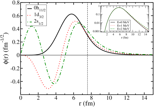
Figure 3: (Color online) Single-proton wave functions in ¹⁵¹Lu for different channels. The inserted plot shows the wave functions of the $0h_{11/2}$ orbital with different energies derived by changing the depth of the potential. Taken from Ref. [40].

Another feature that has to be considered is the influence (if any) of the $Q$ value upon the formation probabilities. The $Q$ value determines the penetrability and, therefore, the radioactive decay process. The question is whether even the spectroscopic quantities are affected by the $Q$ value. To analyse this we show in the inserted plot of Fig. 3 the wave functions of the $0h_{11/2}$ orbital under different energies. These were obtained in Ref. [40] by changing the depth of the potential. As perhaps expected, the tail of the wave function changes dramatically as a function of the energy of the state or the depth of the potential, leading to dramatically different decay rates. On the other hand, the formation amplitude (or more exactly, the single-particle wave function of the emitting particle) at the nuclear surface is not sensitive to changes in the energy, i.e., in the $Q$ values. This is an important conclusion one can also draw from more complex calculations. It is important in particular in the theoretical description of proton-decay half-lives. If the calculated half-life varies as a function of certain inputs like nuclear deformation, one should carefully analyse the reason behind the variance is due to the change in nuclear structure (proton formation amplitude) or simply the decay $Q$ value which is relatively less sensitive to nuclear structure.

There have been extensive theoretical and experimental efforts studying the rotational bands of proton emitters as well as the influence of triaxiality upon proton decay, particularly ¹⁴¹Ho and the triaxially deformed nucleus ¹⁴⁵Tm, as can be found in Refs. [41, 42, 43]. $\gamma$ rays from excited states feeding proton-emitting ground- or isomeric-states have been observed in ¹¹²Cs [44], ¹¹⁷La [45], ¹⁷¹Au [46], and ¹⁵¹Lu [47, 39]. A multiparticle spin-trap $19^{-}$ isomer was discovered in ¹⁵⁸Ta in Ref. [48]. The state is unbound to proton decay but shows remarkable stability. Structure calculations have been carried out for those nuclei. In Ref. [49] the rotational band in ¹⁴¹Ho is described using the projected shell model by taking deformed Nilsson quasi-particle orbitals as bases. The ¹⁴⁵Tm is well described as the coupling of deformed rotational core and the odd proton within the particle-rotor framework in Ref. [50]. In Ref. [51] the Schrödinger equation corresponding to a triaxial potential was solved by using a coupled-channel approach. It was thus shown that the angular distribution corresponding to transitions to the ground state is not sensitive to nuclear structure details, a feature which is at variance with the $\alpha$-decay case. Instead, the decay width is very sensitive to triaxial deformations. It was thus concluded that proton decay is a powerful tool to determine spin, as well as to uncover triaxial shapes in nuclei. These studies reveal the importance of proton decay as a deeper probe for nuclear structure properties.

The proton formation probability can indeed depend upon the deformation of the decaying nucleus. In a well-deformed nucleus the decay can proceed through one of the spherical components of the deformed orbit, which can be very small in the case of large deformations. Therefore the formation probability will be small. As a result, the decay will be very much hindered. On the contrary, in spherical or weakly deformed nuclei the decay proceeds through the only component that is available or the large component and, as a result, the formation probability is large. Therefore proton decay is an important tool to investigate nuclei which cannot be reached otherwise, especially nuclei which are beyond the drip lines. For example, the decay of the $h_{11/2}$ component of the Nilsson orbital $11/2^{-}[505]$ will not be as hindered as the decay from other smaller components.

An interesting case is the proton decay from the nucleus ${}^{109}_{53}$I [52] for which the lowest collective band starting from $7/2^{+}_{1}$ and the inner-band E2 transition properties are observed to be very similar to those of ground state band in the even-even nucleus ¹⁰⁸Te with one less proton [53] as well as those of the $7/2^{+}_{1}$ band in ${}^{109}_{52}$Te [54]. Such a similarity indicates that the odd proton in ¹⁰⁹I, which occupies the $g_{7/2}$ orbital, is weakly coupled to the ¹⁰⁸Te daughter nucleus like a spectator. This simple scheme is also supported by complex large-scale shell-model and pair truncated shell model calculations [55]. The ground state of ¹⁰⁹Te is predicted to be dominated by the coupling of a $d_{5/2}$ neutron to ¹⁰⁸Te. Based on systematics of proton decay half-lives [40] and the level structure of I isotopes from Ref. [56], a similar $5/2_{1}^{+}$ state is also expected to be the ground state of ¹⁰⁹I. However, it was not seen in the life-time measurement of Ref. [52].

Another interesting topic is the competition between $\alpha$ and proton decays from the same nucleus. This has been observed in several nuclei including ¹⁸⁵Ti, ¹⁷⁷Tl and ¹⁷¹Au [57, 58, 46]. There is no microscopic model description of that competition available so far. In addition, the significantly hindered proton decay from the intruder $1/2^{+}$ state in ¹⁸⁵Ti has been observed in Ref. [59].

3.2 Semi-empirical description of proton radioactivity

A simple formula to evaluate the half live of a mother nucleus against proton decay was presented in Refs. [60, 32]. This formula enables the precise assignment of spin and parity for proton decaying states. The only quantities that are needed are the half-life of the mother nucleus and the proton $Q$ value. As a function of these quantities, corrected by the centrifugal barrier, the experimental data of proton emitters with Z$>$ 50 lie along two straight lines which are correlated with two regions of quadrupole deformation. This can be used in experimental searches in a manner similar as the Geiger-Nuttall (GN) law for alpha decay is used.

Within the R-matrix framework, the logarithm of the decay half-life can be approximated by the so-called universal decay law (UDL) as [40]

$$\log T_{1/2} = a\chi^{\prime}+b\rho^{\prime}+dl(l+1)/\rho^{\prime}+c,$$ (12)

where $a$, $b$, $c$ and $d$ are constants determined by fitting available experimental data. $\chi^{\prime}=A_{pd}^{1/2}Z_{p}Z_{d}Q_{p}^{-1/2}$, where $A_{pd}=A_{d}A_{p}/(A_{d}+A_{p})=A_{d}/(A_{d}+1)$ and $Q_{p}$ is the proton Q-value. $\rho^{\prime}=\sqrt{A_{pd}Z_{p}Z_{d}(A_{d}^{1/3}+A_{P}^{1/3})}=\sqrt{A_{pd}Z_{d}(A_{d}^{1/3}+1)}.$ The coefficients $a$ to $d$ can be determined by fitting available experimental data. The UDL was firstly proposed to describe $\alpha$ and cluster decays (see below). It turns out to work well also for proton decays and fission.

The corresponding calculations reproduce well available experimental data, as illustrated in Fig. 4 where the upper panel depicts the quantity $\log T^{{\rm Expt.}}_{1/2}-[b\rho^{\prime}+dl(l+1)/\rho^{\prime}+c]$ as a function of $\chi^{\prime}$. In the lower part of that Figure, the discrepancy between experimental and calculated half lives, i.e., the ratio ${\cal R}=T^{{\rm Expt.}}_{1/2}/T^{{\rm Cal.}}_{1/2}$, is plotted as a function of the emitter charge numbers $Z$. It is seen that most of the data can be reproduced by the calculation within a factor of 4, i.e., with $0.25\leq{\cal R}\leq 4$. Larger discrepancies are seen for emitters between $63\leq Z\leq 67$ and the isomeric $h_{11/2}$ hole state in the $Z=81$ nucleus ¹⁷⁷Tl, where the experimental decay half life is underestimated by the calculation by a factor of about 8.

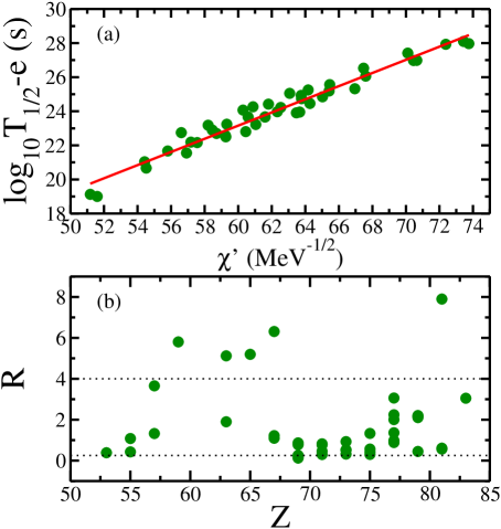
Figure 4: (Color online) Upper: UDL description of proton decay half-lives. Dots are experimental values. $e$ is given by $e=b\rho^{\prime}+dl(l+1)/\rho^{\prime}+c$. Lower: The ratio ${\cal R}=T^{{\rm Expt.}}_{1/2}/T^{{\rm Cal.}}_{1/2}$ as a function of the charge number $Z$. Taken from Ref. [40].

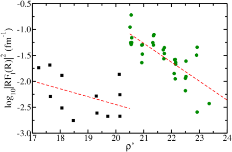
Figure 5: (Color online) The logarithm of the proton-decay formation probabilities $\log_{10}|RF_{l}(R)|^{2}$ extracted from experimental data as a function of $\rho^{\prime}$ from [40]. Squares correspond to nuclei with $N<75(Z\leq 67)$ while circles are for $N\geq 75(Z>67)$.

The proton formation amplitudes $F_{l}(R)$ were extracted from the experimental half lives in Ref. [40] by taking $R=1.2(A_{d}^{1/3}+1)$. They are plotted in Fig. 5 as a function of $\rho^{\prime}$, where one can notice two clearly defined regions. The region to the left of the figure corresponds to the decays of well deformed nuclei where the decay mostly involve small and low $l$ components of the deformed single-particle orbital. The proton formation probabilities decreases for these nuclei as $\rho^{\prime}$ increases. Then, suddenly, a strong transition occurs at the nucleus ${}^{144}_{~{}69}$Tm at $\rho^{\prime}$=20.5. Here the formation probability acquires its maximum value, where the experimental uncertainty regarding the half-life (from where the formation probability is extracted) is still quite large, and then decreases again as $\rho^{\prime}$ increases. The reason of the tendency of the formation probability in the figure is related to the influence of the deformation as discussed above: In the left region of Fig. 5, the decays of the deformed nuclei proceed through small spherical components of the corresponding deformed orbitals and, therefore, the formation probabilities are small. The right region of Fig. 5 involves the decays of spherical orbits as well as major spherical components of deformed orbitals which give large proton formation amplitudes.

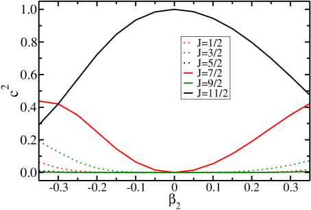
Figure 6: (Color online) The squares of the expansion coefficients $c$ in terms of spherical components for the Nilsson orbit $1/2[550]$ in ¹⁴⁵Tm as a function of deformation $\beta_{2}$ calculated with the deformed Woods-Saxon potential.

The deformed single-particle orbital can be expanded in terms spherical harmonic oscillator single-particle wave functions. As an example, in Fig. 6 we show the expansion of the $\Omega=1/2$ state, i.e., $1/2[550]$ out of $h_{11/2}$, where many orbits with $j\leq\Omega$ contribute. It is seen that the largest components correspond to the $h_{11/2}$ and $f_{7/2}$. The decay of the $f_{7/2}$ component can be favoured due to the smaller centrifugal barrier although the corresponding coefficient is relatively smaller.

In the BCS approach the formation amplitude at a given radius $R$ is proportional to the product of the occupancy $u$ times the single-proton wave function $\psi_{p}(R)$. Therefore the tendencies seen in Fig. 5 may be due to the BCS amplitudes or the radial wave functions. In Fig. 7 the formation probabilities $|F_{l}(R)|$ extracted from experiment for the case of proton decays corresponding to nuclei with $N\geq 75(Z>67)$ are plotted as a function of $u$. The $u$ values were calculated by using a Woods-Saxon potential with the universal and Cherpunov parameters which give similar results. A striking feature is that the values of of the formation probabilities increases with $u$. One can thus conclude that the fluctuations in the experimental formation amplitudes found above for nuclei with $N\geq 75$ are mainly due to fluctuations of the $u$ values. It is also true for cases which departs from the UDL and correspond to the decays of hole states. This occurs in the isomeric state of ¹⁷⁷Tl (as already pointed out above) and also in the ground state of ¹⁸⁵Bi.

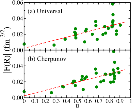
Figure 7: (Color online) The formation amplitudes $|F_{l}(R)|$ extracted from experimental data for proton decays of nuclei $N\geq 75(Z>67)$ as a function of $u$ calculated from BCS calculations using different Woods-Saxon mean fields. From Ref. [40].

4 Two-proton decay

One would expect that the most likely form of two-nucleon decay is the emission of deuterons, which are bound and would be as easy to detect as protons. However that is not the case since so far there is no known nucleus that emit deuterons. In other words, the deuteron Q-value is always negative for all known nuclei. Although proton decay exists the decaying nucleus becomes stable against deuteron decay due to the large binding energy of the added neutron. One may argue that this feature would be even more conspicuous in the decay of $\alpha$-particles, with two neutrons on top of two-protons. The reason why this is not the case is that the binding energy of the $\alpha$-particle is very large, with a value of $B_{\alpha}$ = 28.3 Mev. The deuteron, instead, has a binding energy of $B_{d}$=2.2 MeV. This hughe difference in binding energies explains why $\alpha$-decay is the most likely form of particle radioactivity. As an example one may consider the classical example ²¹²Po(gs) $\rightarrow\alpha$+²⁰⁸Pb(gs). The Q-value in this case is $Q_{\alpha}$=8.95 MeV. Instead for a deuteron decaying from ²¹²Po(gs), i. e. ²¹²Po(gs) $\rightarrow d$+²¹⁰Bi(gs; $1^{-}$) the Q-value is $Q_{d}$=-8.6 MeV. One sees that if the deuteron would have had the same binding energy as the alpha particle, then it would decay from ²¹²Po(gs) with a Q-value of 17.5 MeV, which is nearly double as much as the one carried by the $\alpha$-particle. It is worthwhile to point out that in this hypothetical case the deuteron decay would be somehow hindered by the small $l=1$ centrifugal barrier.

The same mechanisms that forbid the decaying of deuterons also prevent ³H (triton) and ³He decays. This remarkable feature was already noticed in Ref. [61]. In this pioneering paper, in which one- as well as two-proton decay processes were predicted, Goldansky pointed out that a very curious effect emerges, namely that in isotopes which are stable against proton and alpha decay, two-proton decay may be observed. Therefore two-proton radioactivity is a very exotic mode of decay which is energetically possible in some nuclei lying beyond the proton drip line only. The ⁶Be nucleus is the lightest two-proton ground-state emitter with a $Q$ value $Q_{2p}=1.372$ MeV. Moreover, since the Coulomb barrier would hinder the decay of protons one expects that two-proton decay will be possible only in light and medium nuclei [62, 30, 63], including ⁶Be, ⁷B (1.42 MeV), ⁸C (2.11 MeV) and ¹²O (1.638 MeV) where the numbers in the brackets are the corresponding $Q_{2p}$ values extracted from Ref. [64]. On the experimental side, the 2p decay was firstly observed in ⁴⁵Fe [65, 66] and then in ¹⁹Mg[67], ⁴⁸Ni [68, 69] , ⁵⁴Zn [70, 71], and ⁶⁷Kr[72]. The possible observation of two-proton decay from intermediate-mass nuclei was discussed recently in Ref. [73].

As in all forms of radioactive particle decay the two-proton decay rates are expected to be extremely sensitive to the corresponding separation energy (that is to the two-particle Q-value) and therefore a reliable estimate of the Q-values would give a measure of the possibility that the two-proton decay channel is dominant. This was the main theme in one of the first microscopic treatments of two-proton decay [74]. Within the framework of the shell model the process of direct two-proton decay of nuclei with $Z=22-28$ on the proton drip line was considered. On the basis of $0d_{3/2}-0f_{7/2}$ shell-model mass extrapolations the nuclei ³⁹Ti, ⁴²Cr, ⁴⁵Fe, ⁴⁸Ni and ⁴⁹Ni were found to be bound to single-proton decay but unbound to two-proton decay. The spectroscopic factors and lifetimes were evaluated assuming that the decaying two protons are clustered with an internal motion of the two protons (diproton) in a $0s$ state. Using the so-called cluster overlap approximation [75], which essentially consists of the overlap of the two-proton shell-model wave function with the diproton cluster wave function, all spectroscopic factors are near unity. This is not in agreement with experimental data. One failure maybe related to the evaluated binding energies. The diproton approximation may also be incorrect. All these will be important in the developments that follows, as seen below.

A similar calculation was performed in Ref. [76], but with the improvement that the shell model treatment of all nuclei in the study were done coherently. In particular, the Coulomb energy shifts were computed using the same shell model space and interaction for both the “purely” fp-shell and the cross-shell nuclei. This maybe the reason why the results here are more in agreement with experimental data than in [74]. Thus, it was correctly predicted that ⁴⁵Fe was a good candidate to be observed experimentally.

Another similar calculation but performed within the framework of the Hartree-Fock-Bogoliubov and relativistic mean field, including various effective interactions, was performed in Ref. [77]. Here the main conclusion regarding two-proton emission was that diproton emission half-lives depend mainly on the two-proton separation energy and very weakly on the intrinsic structure of diproton emitters. It was also found a very weak dependence of the decay width upon the details of the proton potential. The paper concludes by stating that the results of the calculations justifies the simple estimates of the Refs. [74, 76] mentioned above.

An approach that relies on the properties induced by the pairing interaction upon the ground state of decaying even-even nuclei was introduced in Ref. [78], where the decays of ⁴⁵Fe and ⁵⁸Ni were analysed. The determining variables in this treatment are the distances $r_{1}$ and $r_{2}$ of the protons from the centre of the mother nucleus, and the angle $\theta$ between the corresponding vectors $\vec{r}_{1}$ and $\vec{r}_{2}$. The formalism takes into account that due to the pairing interaction the two protons are clustered on the surface of the mother nucleus. At the same time one uses the property that the protons occupy paired states. Therefore initially they are at the same distance from the centre of the mother nucleus and carry the same energy. The evolution of these three degrees of freedom, i. e. $r_{1}$, $r_{2}$ and $\theta$, are followed according to the dynamics determined by the Schrödinger equation. It was thus found that the half lives are strongly dependent upon the strength of the pairing interaction (see Figs. 7 and 8 of Ref. [78]). That is, two-proton decay is an excellent tool to probe the pairing force. An important prediction is that the decay width is strongly peaked around the symmetric configuration $r_{1}=r_{2}$, in the angle interval $\theta=45^{o}\pm 2^{o}$.

Although these calculations treat correctly the spectroscopic quantities related to the mother nuclei, the decaying process itself, including the relative motion of the decaying two protons, was inadequate. A proper treatment of this starts by noticing that the two-proton decay process may occur through three possible mechanisms: (i) sequential emission of protons via an intermediate state (this was called ”democratic decay” in Ref. [79], a name used by some authors afterwards), (ii) simultaneous emission of protons and (iii) diproton emission, as the one already discussed above, i.e. emission of a ²He cluster with very strong pp correlations.

It is difficult to distinguish experimentally among these decay possibilities. Thus, one of the first observation of two-proton emission was the decay from a narrow resonance at 7.77 MeV in ¹⁴O [80]. In Fig. 4 of that paper the two-proton decay is seen to proceed as a sequential emission. Instead, in the two-proton decay of ³¹Ar [81] the simultaneous emission of the two protons fits the data well. But sequential decays might also describe the experimental data. The $\beta$-delayed two-proton emission from ²²Al was observed recently in Ref. [82]. Based on Monte Carlo simulations, they claim that the involved two-proton decay (from the excited states of ²²Mg to ²⁰Ne) can be explained as a mixture of di-proton and sequential decays.

Another example is the decay of ¹⁸Ne($1^{-}$), which is a resonance lying at 6.15 MeV [83]. As clearly seen in Fig. 4 of this paper the experimental data does not differentiate between diproton ²He emission and direct three-body decay (which here is called ”democratic decay”). The possible diproton decay from ¹⁷Ne was studied in Ref. [84] where an upper limit for the decay width is provided. The two-proton decay from the first excited state of ¹⁶Ne($2^{+}$) was reported in Ref. [85, 86], which again showed patterns of both sequential and prompt two-proton decays. The sequential decay from that nucleus was calculated in a simple potential model in Ref. [87] and in Ref. [88]. The unbound ¹⁵Ne was observed in Ref. [89].

The prominent feature in these examples is that the experiments guide the theoretical undertakings carried out to describe this complicated decay mode. An example of this is the decay from ⁴⁵Fe, which was measured at Ganil [65] and GSI [66]. The decay from ⁵⁴Zn was also measured at Ganil [70] were even the previous results corresponding to ⁴⁵Fe could be confirmed [90]. A detailed report of the experimental efforts can be found in Ref. [91]. In order to describe these decays in Ref. [92] a diproton emission was assumed, which from a theoretical viewpoint is the simplest form of decay among the three cases mentioned above. The results of the calculation agree well with the experimental data if some reasonable assumptions are fulfilled. In Ref. [72], the 2p decay from ⁶⁷Kr was observed. The decay energy was determined to be 1690(17) keV, the 2p decay branching ratio is 37(14)%, and the half-life is 7.4(30) ms which is considerably below earlier theoretical expectations. The observation of prompt 2p decay in that experiment was questioned in Ref. [93]. Meanwhile, in Ref. [94] it was argued that 2p decay can be significantly increased by the deformation effect which leads to a deformed $Z=36$ subshell and large $l=1$ proton components at large oblate deformation. Such expectations should be compared with nuclear structure model calculations.

A more rigorous treatment of the decay should consider the two-proton emission within a realistic three-body model. This was proposed in Ref. [95]. In this model the hyper-spherical harmonic method formulated in Ref. [96] is used. Within this formalism, which includes all two-proton decay modes, the “diproton” model is compared with the three-body calculation corresponding to the decay from the ground states of ¹⁹Mg and ⁴⁸Ni. It was found that the decay width provided by the diproton model is much larger than the one predicted by the three-body calculation, as seen in Fig. 2 of Ref. [95]. As we will see below, this limitation of the diproton model is not seen in all cases. This three-body model was used to analyse a large number of two-proton decay cases in the past [97, 98, 99, 100] and even at present (see Ref. [101] and references therein). This is because the formalism contains all ingredients determining the decay process. However its application is not easy, which explains why mainly only one group uses it, as can be gathered from the references regarding this method.

A number of other approaches have been proposed. In Ref. [102] a time-dependent method was employed to analyse the role played by diproton correlation in two-proton decay from the proton reach isotope ⁶Be. The two-proton emission is described as a time evolution of a three-body metastable state. Introducing a realistic model Hamiltonian which reproduces well experimental two-proton decay widths it was shown that a strongly correlated diproton emission is a dominant process in the early stage of the two-proton emission. When the diproton correlation is absent, the sequential two-proton emission competes with the diproton emission, and the decay width is underestimated. This feature shows that the diproton model may not be as limited as indicated by the three-body model mentioned above. In Ref. [103] the same time-dependent treatment of ⁶Be is applied to analyse the influence of a schematic density dependent pairing force. It is found that with such simple pairing force it is impossible to describe simultaneously the two-proton decay width, the two-proton Q-value and the two-nucleon scattering length. It is concluded that to achieve a complete agreement with all those experimental quantities the pairing force has to be elaborated farther. But this would harm considerably the simplicity of the model and no additional development took place.

Since the two protons in the decay process may be trapped within the mother nucleus during a long time, one may expect that long-lived mother nuclei should show a halo corresponding to the two protons orbiting the daughter nuclei before decaying. This was analysed in Ref. [104].

Another related subject is the possible existence of two-neutron decay and even tetra-neutron resonance. Those states can be analysed in principle in the same framework as mentioned above but influence of the continuum may become more important there.

Concluding this Section one sees that two-proton decay has shown to be a powerful tool to study properties of nuclei lying on and beyond the proton drip line.

5 $\alpha$ decay

There have been long-standing experimental interest in conducting nuclear alpha decay studies which not only carry important information on nuclear structure but are also very useful even today for isotope identification via $\alpha$-decay tagging [105, 106, 107, 108, 109, 110, 111, 112, 113]. Moreover, the importance of $\alpha$ particle capture reactions (or the inversed $\alpha$-decay process) for nucleosynthesis has been investigated during a long time. One of the most prominent cases in this line is the famous ${\alpha}$-capture to the so-called Hoyle state in ¹²C, which is essential to the nucleosynthesis of carbon. The direct 3$\alpha$ decay or breakup from ¹²C has been measured recently in Refs. [114, 115], which provides constraints for the many theoretical models, both microscopic and empirical, that have been applied to study the clustering property of the nucleus.

Most $\alpha$ emitters concern proton-rich or neutron-deficient nuclei. In principle, it can also be relevant for the astrophysical rapid neutron capture process (r-process) in actinides like Pb and Bi [116] and in superheavy nuclei [117]. The competition between fission and $\alpha$ decay under typical r-process conditions was studied recently in Refs. [118, 119]. The relevance of $\alpha$ decay of ²¹⁰Po in the termination of the slow neutron capture process (s process) was re-measured recently in Ref. [120].

As already pointed out in the Introduction $\alpha$-decay is not only the most common of all particle decay processes but it is also, through the understanding of the penetration of the $\alpha$-particle through the coulomb and centrifugal barriers, the most important event that confirmed the probabilistic interpretation of quantum mechanics. The amount of work related to this subject is huge but there have also been many reviews describing that work. Among the latest of these is Ref. [16]. Here we will only report the advances that took place in this field since that time. There have been significant developments during this period, in the microscopic as well as in the effective approaches to this problem. We will first report the microscopic developments.

5.1 The microscopic description of $\alpha$ decay

Before entering into the developments of this difficult and fascinating subject during the last decades we will very briefly describe the background upon which those developments are founded.

The microscopic treatment of $\alpha$-decay started with the study of scattering processes where a compound nucleus may decay into channels $c$ and $c^{\prime}$. For our purposes the main feature of these studies was the parametrization of the corresponding S-matrix as formulated in Ref. [121]. The resulting Breit-Wigner formula reads,

$$S_{cc^{\prime}}=\delta_{cc^{\prime}}-i\frac{\Gamma_{c}^{1/2}\Gamma_{c^{\prime}}^{1/2}}{{\cal E}-E+i\Gamma/2}$$ (13)

where $E$ and $\Gamma$ are the position and width of the resonance induced by the trapping of the compound nucleus before decaying into the various open channels. The decay into channel $c$ is characterized by the partial decay width $\Gamma_{c}$. Therefore the total width is $\Gamma=\sum_{c}\Gamma_{c}$.

The poles of the S-matrix are the complex energies ${\cal E}=E-i\Gamma/2$. At these energies the compound nucleus lives a mean time $T=\hbar/\Gamma$. Since the nucleus decays the corresponding incoming wave is negligible compared with the outgoing wave. At the limit of an infinite value of $T$ the width vanishes and the compound nucleus is bound.

Eq. (13) was based on an intuitive argument. A strict quantum mechanics derivation of this formula was performed within the framework of the R-matrix theory in Ref. [9]. As pointed out in the Introduction, this formalism was used by Thomas to derive the expression of the $\alpha$-decay width given by Eq. (1).

For the case of $\alpha$-decay the formation amplitude of the alpha particle is given by

$${\cal F}_{c}(R)=\int d{\mathbf{R}}d\xi_{d}d\xi_{\alpha}[\Psi_{d}(\xi_{d})\phi(\xi_{\alpha})Y_{l}(\mathbf{R})]^{*}_{J_{m}M_{m}}\Psi_{m}(\xi_{d},\xi_{\alpha},\mathbf{R}),$$ (14)

where $\xi_{d}$ and $\xi_{\alpha}$ are the internal degrees of freedom determining the dynamics of the daughter nucleus and the $\alpha$-particle respectively. The wave functions $\Psi_{d}(\xi_{d})$ and $\Psi_{m}(\xi_{d},\xi_{\alpha},\mathbf{R})$ correspond to the daughter and mother nuclei. The $\alpha$-particle wave function has the form of a $n=l=0$ harmonic oscillator wave function in the neutron-neutron relative distances $r_{nn}$, as well as in the proton-proton distance $r_{pp}$ and in the distance between the mass centres of the $nn$ and $pp$ pairs $r_{np}$, i. e. [122],

$$\phi(\xi_{\alpha})=\sqrt{\frac{1}{8}}(\frac{\nu_{\alpha}}{\pi})^{9/4}exp[-\nu_{\alpha}(r_{nn}^{2}+r_{pp}^{2}+2r_{pn}^{2})/4]\xi_{\alpha}$$ (15)

where $\xi_{\alpha}$ is the $\alpha$-spinor corresponding to the lowest harmonic oscillator wave functions. That is the orbital angular momenta are $l_{nn}$=$l_{pp}$= $l_{np}$=0 and the same for the spin part. Therefore the total angular momenta are $L=S=0$. The quantity $\nu_{\alpha}$ is the $\alpha$-particle harmonic oscillator parameter.

The calculation of the formation amplitude (14) is the most difficult task in the evaluation of the width. From a microscopic point of view one has to be able to describe the mother wave function well outside the nuclear surface, where at the matching point $R$ only the Coulomb interaction is present. During a time in the early 1970’s there was a long argument about the importance of the Pauli principle acting upon nucleons in the $\alpha$-cluster and those in the daughter nucleus [123]. But eventually it was shown that the influence of Pauli exchanges is negligible at these long distances. For details see e. g. Ref. [16].

The most difficult challenge in the calculation of the formation amplitude is to describe properly the small but crucial daughter times $\alpha$-cluster component in the mother wave function $\Psi_{m}(\xi_{d},\xi_{\alpha},\mathbf{R})$. As seen from Eq. (14) it is this component that contributes to the formation amplitude. In other words one should be able to describe at the point $R$ the clustering of the four nucleons that eventually becomes the $\alpha$-particle. This task was pursued by many researches [16]. While struggling with this problem a number of other important nuclear properties where found. Below we will present these developments which occur through studies performed within the two most current microscopic frameworks, namely the shell model and the BCS theory.

5.2 Shell model treatment of the formation amplitude

The shell model provides an excellent representation to describe nuclear properties. In the case of the $\alpha$-formation amplitude the main region that such representation should describe is at the matching point $R$, as discussed above. Therefore the representation should include states which are not negligible at such distances. One thus sees from the beginning that high lying single-particle states, which extend far out in space, should be an important part of the shell-model representation. But this representation should also be able to describe the clustering of the four nucleons that constitute the $\alpha$-particle. Here is the core of the problem facing microscopic calculations of cluster decay.

The problem of describing processes on the nuclear surface is old. At the beginning of two-particle transfer studies one faced the same problem. The calculation of the two-particle transfer cross section required a precise knowledge of the corresponding form factor on the target nuclear surface. Since the asymptotic behaviour of the form factor is determined by the two-particle separation energy one chose as binding energy for all single particle states half that energy [124, 125]. This gave rise to the introduction of the Sturm-Liouville representation to describe processes occurring on the nuclear surface. In this representation one uses eigenstates of a realistic central potential, e. g. Woods-Saxon, which has eigenvalues with proper asymptotic behaviour. But all these eigenstates are evaluated at the same bound energy, for instance at half the energy of the pair of nuclei to be transferred. Details about the Sturm-Liouville representation can be found in Ref. [126]. Although this representation is well suited to describe the asymptotic behaviours of nuclear functions, its application is not very convenient as compared with harmonic oscillator (ho) representations. Besides the easiness of dealing with ho eigenfunctions, they allow one to evaluate the $\alpha$ formation amplitude analytically. This is because the $\alpha$-cluster function itself is a product of ho functions. Therefore most microscopic calculations of $\alpha$-decay have been performed by using ho representations. We will see this below. We will also see the advantage of other representations introduced in order to describe processes in the continuum part of nuclear spectra.

The most simple case in the calculation of the formation amplitude (14) is when the numbers of neutrons and protons in the daughter nucleus are both magic numbers. This implies within the shell model that the daughter nucleus has no effect in the formation amplitude if, as it is usually the case, no core excitations are considered. The shell model description of the mother nucleus can be performed in terms of uncorrelated two neutron and two proton states or in term of correlated (physical) ones. This is possible because the uncorrelated and correlated states are related by a unitary (rotational) transformation in the Hilbert space. The preferred decaying nucleus fulfilling these condition is ²¹²Po(gs). The corresponding wave function can then be written within the shell model as,

$$|^{212}{\rm Po}(gs)\rangle=\sum_{\alpha_{2}\beta_{2}}X(\alpha_{2}\beta_{2};gs)|^{210}{\rm Pb}(\alpha_{2})\otimes^{210}{\rm Po}(\beta_{2})\rangle$$ (16)

where $\alpha_{2}$ ($\beta_{2}$) labels two-neutron (two-proton) states. Due to the pairing correlation one expects that in the above expression the components with $\alpha_{2}=gs$ and $\beta_{2}=gs$ are overwhelmingly dominant. Therefore one may write,

$$|^{212}{\rm Po}(gs)\rangle=|^{210}{\rm Pb}(gs)\otimes^{210}{\rm Po}(gs)\rangle$$ (17)

We will give a brief introduction to calculations based in the expansion (17). A review, including references, can be found in [16].

In the first alpha-decay evaluation of ²¹²Po(gs) using this expression was found that the inclusion of many configurations increased the width by many orders of magnitude. This can be understood since on the surface of the nucleus, where the $\alpha$-particle is formed, the continuum part of the single-particle representation (or very high lying shells in a bound representation) is important. But even including up to 16 major harmonic oscillator shells the absolute decay width was smaller than the experimental one in spherical nuclei [122].

It was also found that the huge increase of the decay width with increasing number of configurations was mainly due to the clustering of the two neutrons and two protons induced by the valence shells. The pioneers in $\alpha$-decay [127] already suspected that the increase of the decay width with the number of configurations was due to the clusterization thus described. But it has to be noticed that higher lying shells contribute to the clustering to a lesser extent [128].

Yet with all shells included, that is the valence plus the high lying shells, the decay width was still too small by one order of magnitude. Taken into consideration only one configuration in Eq. (17) implies that the neutron-proton interaction is neglected. To correct this deficiencies other configurations (such as $|^{210}{\rm Pb}(2^{+}_{1})\otimes^{210}{\rm Po}(2^{+}_{1})\rangle$) were also taken into account, but the corresponding calculations did not improve significantly. This is expected since neutrons and protons occupy different major shells with different parity and the neutron-proton interaction matrix elements are therefore hampered. In view of these drawbacks it was assumed that the only possibility left to increase the calculated value of the width was to include the nuclear continuum, and the neutron-proton clustering, in a more realistic fashion than the one provided by the bound ho states. This we will review below.

The evaluation of $\alpha$ formation amplitude involves the evaluation of the overlap between the corresponding proton and neutron radial functions in the laboratory framework with the $\alpha$-particle intrinsic wave function as defined in the centre of mass framework (see, e.g., Ref. [129]). The transformation can be relatively easily handled if the radial wave functions are defined within the harmonic oscillator basis due to its intrinsic simplicity. This is also the season that the harmonic oscillator representation is used in most ab initio and shell-model configuration interaction calculations. More realistic calculations have been based on phenomenological Woods-Saxon and Nilsson single-particle single-particle states. A single particle basis consisting of two different harmonic oscillator representations was introduced in Ref. [130]. An additional attractive pocket potential of a Gaussian form was introduced on top of the Woods-Saxon potential in Ref. [131] in order to correct the asymptotic behaviour of the $\alpha$ formation amplitude. The mixture of shell model and cluster wave functions was considered in Ref. [132] and was applied to describe the decay of the ground state of ²¹²Po. the amount of core + clustering in the parent state and the corresponding spectroscopic factor that can reproduce experimental decay half-life are found to be 0.30 and 0.025, respectively.

Figure 8: The square of the two-boday wave function $|\Psi_{2}(r_{1},r_{2},\theta)|^{2}$ with $r_{1}=9$ fm for the two protons in ²¹⁰Po calculated within one orbital (left) and with all shells (right). Taken from Ref. [133].

The fundamental role of configuration mixing was only confirmed by actual large-scale calculations [122, 134, 133]. The physics behind the enhancement induced by configuration mixing is that, with the participation of high-lying configurations, the pairing interaction clusters the two neutrons and the two protons on the nuclear surface, as can be seen from Fig. 8 where the calculated two-body wave function $|\Psi_{2}(r_{1},r_{2},\theta)|^{2}$ for the two protons in ²¹⁰Po within model spaces containing one orbital and all the orbitals above $Z=82$ are compared. This wave function has the form,

$$\Psi_{2}(r_{1},r_{2};\theta_{12})=\frac{1}{4\pi}\sum_{p\leq q}\sqrt{\frac{2j_{p}+1}{2}}X(pq;{\rm gs})\varphi_{p}(r_{1})\varphi_{q}(r_{2})P_{l_{p}}(\cos\theta_{12}),$$ (18)

where $\varphi$ is the single-particle wave function and $P_{l}$ is the Legendre polynomial of order $l$ satisfying $P_{l}(\cos 0)=1$ (notice that for the ground states studied here it is $l_{p}=l_{q}$). The two-neutron and two-proton wave-function terms add up constructively in the surface region when many shells are involved. It was found that the mechanism that induces clustering is the same that produces the pairing collectivity, which is manifested in an strong increase in the form factor corresponding to the corresponding transfer cross section. This property gives rise to a giant pairing resonances (see below), which corresponds to the most collective of the pairing states lying, as the standard (particle-hole) giant resonances, high in the spectrum.

Figure 9: The square of the two-boday wave function $|\Psi_{2}(r_{1},r_{2},\theta)|^{2}$ with $r_{1}=9$ fm for the two neutrons in ²¹⁰Pb (left) and two neutron holes in ²⁰⁶Pb (right). Taken from Ref. [133].

For non-degenerate systems the pairing collectivity manifests itself through the correlated contribution from many configurations, which is induced by the non-diagonal matrix elements of the pairing interaction in a shell-model context. For two particles in a non-degenerate system with a constant pairing, the energy can be evaluated through the well known relation [135],

$$G\sum_{i}\frac{2j_{i}+1}{2\varepsilon_{i}-E_{2}}=2.$$ (19)

The corresponding wave function amplitudes are given by

$$X_{i}=N_{n}\frac{2j+1}{2\varepsilon_{i}-E_{2}}$$ (20)

where $N_{n}$ is the normalization constant. All amplitudes $X_{i}$ contribute to the two-particle clustering with the same phase due to the strongly attractive nature of the pairing interaction. The correlation energy induced by the monopole pairing corresponds to the difference

$$\Delta^{(3)}_{C}=\varepsilon_{\delta}-\frac{1}{2}E_{2},$$ (21)

where $\delta$ denotes the lowest orbital. As the gap $\Delta$ increases the amplitude $X_{i}$ becomes more dispersed, resulting in stronger two-particle spatial correlation. This difference, or more exactly $\Delta-1/2G$ with the self energy removed, is an important measure of the two-particle spatial correlation at the surface, reflected in a corresponding clustering of the two nucleons forming the pair (see, e.g., Ref. [133]). This clustering induces an increase in the strength of the corresponding pair-transfer reaction.

In Fig. 9 we compared the two-neutron wave functions of ^210,206Pb. A striking feature thus found is that the two-neutron correlation is significantly larger in ²⁰⁶Pb than in ²⁰⁶Pb in relation to the larger pairing gap in the former case.

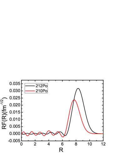
Figure 10: (Color online) The $\alpha$-formation amplitudes $R\mathcal{F}_{\alpha}(R)$ corresponding to the nuclei ²¹²Po(gs) and ²¹⁰Po(gs). Taken from Ref. [133].

Within the shell model The amplitudes $X$ of the four-particle state $\alpha_{4}$ in ²¹²Po vanish if this interaction is neglected. Then only one of the configurations in Eq. (16) would appear. This is done, for instance, in cases where the correlated four-particle state is assumed to be provided by collective vibrational states. The corresponding formation amplitude acquires the form,

$${\cal F}_{\alpha}(R;^{212}{\rm Po(gs)})=\int d\mathbf{R}d\xi_{\alpha}\phi_{\alpha}(\xi_{\alpha})\Psi(\mathbf{r_{1}}\mathbf{r_{2}};^{210}{\rm Pb(gs)})\Psi(\mathbf{r_{3}}\mathbf{r_{4}};^{210}{\rm Po(gs)}),$$ (22)

where $\mathbf{r_{1}},\mathbf{r_{2}}$ ($\mathbf{r_{3}},\mathbf{r_{4}}$) are the neutron (proton) coordinates and $\mathbf{R}$ is the centre of mass of the $\alpha$ particle.

The decay of the nucleus ²¹⁰Po(gs) leads to the daughter nucleus ²⁰⁶Pb(gs), which is a two-hole state. The formation amplitude becomes,

$${\cal F}_{\alpha}(R;^{210}{\rm Po(gs)})=\int d\mathbf{R}d\xi_{\alpha}\phi_{\alpha}(\xi_{\alpha})\Psi(\mathbf{r_{1}}\mathbf{r_{2}};^{206}{\rm Pb(gs)})\Psi(\mathbf{r_{3}}\mathbf{r_{4}};^{210}{\rm Po(gs)}).$$ (23)

With this expression for the formation amplitude, the experimental half-life can be reproduced if a large number of high-lying configurations is included. The calculated formation amplitude for ^210,212Po are plotted in Fig. 10.

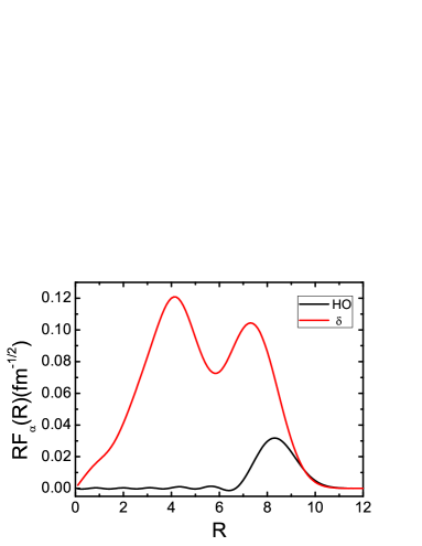
Figure 11: (Color online) Comparison of the $\alpha$ formation amplitude $RF_{\alpha}(R)$ of ²¹²Po calculated from the $\delta$ function approximation and the Gaussian form of the $\alpha$ intrinsic wave function.

If we assume that the intrinsic wave function of the $\alpha$ particle can be approximated by a $\delta$ function, a even simpler expression exist for the $\alpha$ formation amplitude which reads,

$$F_{\alpha}(R)=\frac{16\pi^{2}}{R^{4}}\left(\frac{s_{\alpha}^{3}}{3}\right)^{3/2}\Phi_{2\pi}(R,R,0)\Phi_{2\nu}(R,R,0),$$ (24)

where $S_{\alpha}=\sqrt{20}/3R_{\alpha}$ and we take $\mathbf{\hat{r}_{1}}=\mathbf{\hat{r}_{3}}=\mathbf{\hat{z}}$. In Fig. 11 we plotted the formation amplitude evaluated with this approximation, in comparison with that calculated with the realistic $\alpha$ intrinsic wave function. The $\delta$-function approximation ignores the fact that the four nucleons forming the $\alpha$ particle only strongly clustered at the nuclear surface and overestimates strongly the $\alpha$ particle formation probability inside the nucleus. It may be interesting to point out here that the result from the simple calculation in Fig. 11 indicates clearly the four body spatial/clustering correlation inside does not necessary mean that $\alpha$ or $\alpha$-like clustering has occurred inside the nucleus. This is one confusion we often see in theoretical studies of nuclear clustering.

5.2.1 Limitations of the shell-model

The shell model has been extremely successful to explain and predict nuclear properties. Features like the structure of nuclear spectra, particularly high-spin states, nuclear reactions, processes in the continuum part of the spectrum, nuclear deformations and so on, could be well explained by the shell model. For a review see Ref. [136]. Even $\alpha$-decay processes, including half lives of excited states and relative decay widths, could be well understood through the shell model as seen in Subsection 5.8. For an early importance of the shell model in $\alpha$-decay see Ref. [16]. Yet, the absolute decay with of the heavy nucleus ²¹²Po(gs) could be calculated only within an order of magnitude. More striking is that the clustering properties of neutrons and protons that constitute the alpha-particle can be explained by the shell-model.

One may argue that it is the difference of neutron and proton numbers in ²¹²Po which is responsible for the shortcomings of the shell-model in explaining the absolute decay width. This is not the case, as shown in the next subsection.

The first experimental indication that the shell model alone could not describe properties in ²¹²Po did not come from $\alpha$-decay probes but rather from electromagnetic transitions. This was done in Ref. [137], where excited states in that nucleus were populated by $\alpha$-transfer using the ²⁰⁸Pb(¹⁸O,¹⁴C) reaction. Their de-excitation $\gamma$-rays were studied and several levels were found to decay by an unique low energy $E1$ transition populating the yrast state with the same spin value. Their lifetimes were measured and it was discovered that the transitions were very enhanced. These results, which could no be explained within the standard shell-model, were found to be consistent with an alpha cluster structure. This gives rise to states with non-natural parity.

As we have described above it had been known for a long time that a necessary requirement to properly describe particle emission and transfer processes is that the basis wave functions follow correct asymptotic values. In $\alpha$-decay this feature seems to be even more remarkable and it is in fact at the origin of the deficient description of the decay process by using the standard shell model. A successful solution of this problem was presented in Ref. [138], where the decaying state was described as a combination of a shell-model wave function plus a cluster component. The important feature of this approach is that the cluster component is expected to take care of the high-lying shell-model configurations and, therefore, the shell-model component is evaluated within a major shell only. The cluster component is expanded in terms of shifted Gaussian, and the coefficients are found by diagonalizing the residual two-body interaction.

This method was applied in Ref. [139] to describe the experimental features of Ref. [137]. By using a shifted Gaussian component in the single-particle wave functions it was possible to describe the $\alpha$-decay process, while the shell-model part of the wave function explained well the corresponding $B(E2)$ transitions.

This deviation of the pure shell model is a disadvantage which would make the shell model less appealing if the mixing of shell model and cluster components should be a general trait. Fortunately it is not. However, attempts were done trying to include the effects induced by the cluster component within a pure shell-model representation. This implies that the standard (e. g. Woods-Saxon) central potential has to be modified. The modification consists in adding an attractive pocket potential of a Gaussian form localized on the nuclear surface. The eigenvectors of this new mean field provides a representation which retains all the benefits of the standard shell model while at the same time reproducing well the experimental absolute $\alpha$-decay widths from heavy nuclei [140]. Although one can in this way obtain results similar to the ones provided by the shell-model plus cluster representation, the application of the method is cumbersome and no farther application was reported. But this confirms the limitations of the shell model in explaining absolute decay widths in $\alpha$-decay.

5.3 Significance and outcome of the Continuum treatment

The study of the influence of the continuum upon alpha decay gave rise to the appearance of new features which are apparently unrelated to the alpha decay process. We will analyze these features case by case.

5.3.1 Giant pairing resonances

The first attempt to consider the continuum in $\alpha$-decay was related to the inclusion of the neutron-proton interaction. As discussed above, the most important states in the formation of the $\alpha$-particle are the isovector $0^{+}$ pairing states, which in our case are ²¹⁰Pb(gs) and ²¹⁰Po(gs), due to their neutron-neutron and proton-proton clustering features. It was therefore assumed that the neutron-proton clustering should also proceed through an isovector pairing neutron-proton state. Such a state cannot be built upon the valence shells in this case, since they correspond to the principal quantum number N=5 for protons and N=6 for neutrons carrying opposite parities. Therefore the lowest isovector pairing neutron-proton state should be formed by protons and neutrons moving in the N=6 shell. This state had not been observed but was assumed to lie at 5 MeV above the ground state, i. e. above the state ²¹⁰Bi($1^{-}$;gs). The corresponding wave function was obtained by using a pairing force, adjusting the pairing strength to fit the energy of the lowest $0^{+}$ state thus calculated to lie at 5 MeV. This wave function showed to have strong clustering features, as expected. Including this state in the basis of Eq. (17) one obtained the alpha clustering as well as the experimental value of the decay width. However, this was accomplished by adjusting the components of the wave function in an unrealistic fashion [141]. But the idea that there should exist a neutron-proton isovector pairing state at high energy in nuclei with proton number differing from the neutron number prompted the possibility of considering this neutron-proton state as the isobaric analog to the neutron-neutron ground state. In our case the state ²¹⁰Bi($0^{+}_{1}$) should be analog to the state ²¹⁰Pb($0^{+}_{1}$;gs). As a result there should be another isobaric analog state corresponding to two-proton excitations. In our case this should be an state lying at about 10 MeV (the gap corresponding to two major shells) above the ground state of ²¹⁰Po(gs). The same should be valid in the nucleus ²¹⁰Pb. Here there should be a collective isovector pairing state at about 10 MeV. This is analog to the particle-hole collective excitations, were e. g. the isovector dipole giant resonance in ²⁰⁸Pb lies at about 10 MeV (the real figure is 13.5 MeV).

To verify the existence of the high lying collective pairing state a calculation was performed by using a pairing interaction and a large single-particle representation [142]. The three isobaric states discussed above were evaluated. The ones in ²¹⁰Bi and in ²¹⁰Po show strong clustering features, even more than in ²¹⁰Pb(gs). They are built mainly upon high lying single-particle states and are strongly excited in two-particle transfer reactions. Therefore they can be considered pairing giant resonances (GPR). In fact this state had been predicted before just as an analogue to the particle-hole giant resonance [143].

The state ²¹⁰Pb(GPR) was also found to be strongly pairing collective lying at an energy 0f 11.4 MeV. This prompted an intense experimental activity looking for this GPR, but without any success [144]. However the calculation of this GPR was later confirmed in an independent work [145]. To probe the importance of the continuum in this very high lying two-neutron state a calculation using the Berggren representation was performed. As will be seen in the next item below, the Berggren representation was also introduced in relation to alpha decay. It is very well fitted to take into account the escape process of particles lying high in the continuum. It was thus found that in the state ²¹⁰Pb(GPR) the neutrons tend to scape the nucleus since there is no Coulomb barrier to trap them. As a result that state is a very wide resonance. Therefore it can be considered a part of the continuum background rather than an observable state [146].

Yet the GPR was still been sought but in lighter nuclei. It was thus proposed that it should exist in the nucleus ¹³²Sn [147]. Finally, signatures of the GPR were found in ¹⁴C and in ¹⁵C [148].

5.3.2 The Berggren representation

The failure of bound representations to explain the width of $\alpha$-decay resonances brought up the question whether the continuum should be included explicitly. An important step in the study of the continuum in many-body problems was given by the introduction of the Gamow resonances [149, 150]. These are solutions of the time-independent Schroedinger equation with purely outgoing waves at large distances. These resonances, together with the proper continuum and bound states, were used by Berggren as a representation to write the single-particle Green function [151]. However the first time that the Berggren representation was applied did not concern alpha-decay but rather particle-hole giant resonances [152]. This was because at that time there were a large amount of experimental data and open questions related to giant resonances and the continuum. But the introduction of the Berggren representation was followed by many applications. It was the origin of what eventually would be called ”Shell model in the complex energy plane” or ”Gamow shell model”. A review of this development can be found in Ref. [153].

This representation was used to evaluate the alpha formation amplitude corresponding ´to the $\alpha$-decay of ²¹²Po(gs) [154]. One thus succeed in describing the clustering up to large distances. For this a large number of configurations had to be included in the representation. However, the maximum value of the formation amplitude was about the same as the one obtained by using a bound representation. As a result, the disagreement between the calculated and experimental alpha decay width persisted.

Yet, in Ref. [155] a similar calculation provided a good agreement with experiment. But this paper was strongly criticized, as incorrect, in Ref. [156]. The authors of [155] answered in [157]. This in fact left the question open on whether the shell model is indeed able to describe absolute decay widths. It seemed that a more radical solution to this problem was needed, as described in the next item below.

5.4 The Geiger-Nuttall law and its generalizations

The huge range of $\alpha$ decay half-lives can be modelled through the Geiger-Nuttall law [158, 159], which shows a striking correlation between the half-lives of radioactive decay processes and the decay $Q_{\alpha}$ values. The decay half life is predicted by this law to be,

$$\log T_{1/2}=\mathcal{A}Q_{\alpha}^{-1/2}+\mathcal{B},$$ (25)

where $\mathcal{A}$ and $\mathcal{B}$ are constants that can be determined by fitting to experimental data. The Gamow theory reproduced the Geiger-Nuttall law very well by describing the $\alpha$ decay as the tunnelling through the Coulomb barrier.

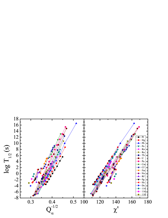
Figure 12: Systematics of $\alpha$ decays from even-even nuclei with $Z=78-118$. The $Q_{\alpha}$ values are in unit MeV. The quantity $\chi^{\prime}$ (in MeV^-1/2) is defined as $\chi^{\prime}=Z_{c}Z_{d}\sqrt{A/Q_{c}}$ (see text). Taken from Ref. [160].

The Geiger-Nuttall law in the form of Eq. (25) has limited prediction power since its coefficients change for the decays of each isotopic series, see Fig. 12. Intensive work have been done trying to generalize the Geiger-Nuttall law for a universal description of all detected $\alpha$ decay events [161, 162]. One of the most known generalization is the Viola-Seaborg law [163] which for even-even nuclei reads

$$\log T_{1/2}=(aZ_{d}+b)Q_{\alpha}^{-1/2}+bZ_{d}+d$$ (26)

where $a$, $b$ and $d$ are constants and $Z_{d}$ the charge number of the daughter nucleus.

The importance of a proper treatment of $\alpha$ decay was attested in Refs. [160, 164] which shows that the different lines can be merged into a single line. In this generalization the penetrability is still a dominant quantity where $H^{+}_{0}(\chi,\rho)$ can be well approximated by an analytic formula

$$H^{+}_{0}(\chi,\rho)\approx(\cot\beta)^{1/2}\exp\left[\chi(\beta-\sin\beta\cos\beta)\right].$$ (27)

By defining the quantities $\chi^{\prime}=Z_{\alpha}Z_{d}\sqrt{A_{\alpha d}/Q_{\alpha}}$ and $\rho^{\prime}=\sqrt{A_{\alpha d}Z_{\alpha}Z_{d}(A_{d}^{1/3}+A_{\alpha}^{1/3})}$ where $A_{\alpha d}=A_{d}A_{\alpha}/(A_{d}+A_{\alpha})$, one gets, after some simple algebra,

$$\log T_{1/2}=a\chi^{\prime}+b\rho^{\prime}+c,$$ (28)

where $a$, $b$, $c$ are constants to be determined.

One thus obtained a generalization of the Geiger-Nuttall law (called UDL) which holds for all isotopic chains and all cluster radioactivities. Eq. (28) reproduces well most available experimental $\alpha$ decay data on ground-state to ground-state radioactive decays.

The UDL works not only for alpha decay but also for proton decay (see above) and heavier cluster decays (see below).

5.4.1 Extraction of the formation probability from experimental half-lives

The success of the Geiger-Nuttall law and UDL is mainly due to the small variations of the $\alpha$-particle formation probability when going from a nucleus to its neighbours, as compared to the penetrability. In the logarithm scale of the Geiger-Nuttall law, the differences in the formation probabilities are usually small fluctuations along the straight lines predicted by that law.

The formation amplitude ${\cal F}_{\alpha}(R)$ can be extracted from the experimental half-lives $T^{{\rm Expt.}}$ corresponding to ground state to ground state transitions

$$\log|R{\cal F}_{\alpha}(R)|=\frac{1}{2}\log\left[\frac{\ln 2}{\nu}|H^{+}_{0}(\chi,\rho)|^{2}\right]-\frac{1}{2}\log T^{{\rm Expt}}_{1/2}.$$ (29)

This was done in Refs. [133, 160, 164, 165, 166]. In Fig. 13 we plotted the formation probability for known alpha decays. They follow roughly a linear behaviour as a function of $\rho^{\prime}$ which is the key for the success of UDL.

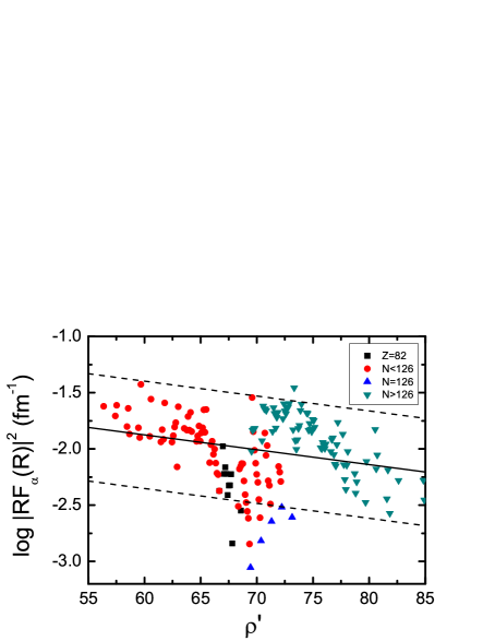
Figure 13: The $\alpha$ decay formation amplitudes $\log|RF(R)|^{-2}$ as a function of the charge number of the mother nucleus $Z$ (left) and $\rho^{\prime}$. Right plot from Ref. [133].

It was found that although the UDL reproduces nicely most available experimental $\alpha$ decay data, as expected, there is a case where it fails by a large factor. This corresponds to the $\alpha$ decays of nuclei with neutron numbers equal to or just below $N=126$ [133, 167], as can be seen from the left panel of Fig. 14 where we plotted the discrepancy between experimental and calculated $\alpha$ half-lives. The reason for this large discrepancy is that in $N\leq 126$ nuclei the $\alpha$ formation amplitudes are much smaller than the average quantity predicted by the UDL. The case that shows the most significant hindrance corresponds to the $\alpha$ decay of the nucleus ²¹⁰Po. It was found that the formation amplitude in ²¹⁰Po is hindered with respect to the one in ²¹²Po due to the hole character of the neutron states in the ²¹⁰Po case. This is a manifestation of the pairing mechanism that induces clusterization, which is favoured by the presence of high-lying configurations (see Sec. 5.6 below). Such configurations are more accessible in the neutron-particle case of ²¹²Po than in the neutron-hole case of ²¹⁰Po. As a result, the neutron pairing correlation and eventually the two-neutron and $\alpha$ clustering are significantly enhanced in ²¹²Po in comparison with those in ²¹⁰Po.

Figure 14: Left: Discrepancy between experimental decay half-lives and UDL calculations as a function of the neutron number of the mother nucleus N.

Figure 15: $log_{10}|RF(R)|^{2}$ for Po (circle) and Rn (triangle) isotopes with $N<126$ (closed symbols) and with $N>126$ (open symbols) as a function of $Q_{\alpha}^{-1/2}$. The dashed lines are to guide the eye. From Ref. [166].

5.4.2 Limitations of the Geiger-Nuttall law

The origin and physical meaning of the coefficients $\mathcal{A}$ and $\mathcal{B}$ in the Geiger-Nuttall law can be deduced by comparing Eq. (25) and (28). These coefficients are determined from experimental data and show a linear dependence upon $Z$. The need for a different linear $Z$ dependence of the coefficients $\mathcal{A}$ and $\mathcal{B}$ in different regions of the nuclear chart was discussed in Ref. [166], which is related to the generic form of the $\alpha$ formation probability as will be discussed just below. When the dependence of $log_{10}|R{\cal F}_{\alpha}(R)|^{2}$ on the neutron number is not linear or constant, the Geiger-Nuttall law is broken. This also explains why the Geiger-Nuttall law works so well for nearly all $\alpha$ emitters known today, as the data within each isotopic chain are limited to a region where $log_{10}|R{\cal F}_{\alpha}(R)|^{2}$ is roughly a constant or behaves linearly with $N$.

We notice that, for the $\alpha$ decays of nuclei with neutron numbers equal to or just below $N=126$, the UDL fails by a large factor but,on the other hand, the normal GN law seems to work, as illustrated in Fig. 16. The fact that the GN law is not “broken” at the first glance, is simply related to the $Q_{\alpha}$ (as well as $Q_{\alpha}^{-1/2}$) values exhibit a quasi linear pattern as a function of rising neutron number when approaching the $N=126$ shell closure. Therefore $log_{10}|RF(R)|^{2}$ and $log_{10}(T_{1/2})$ will still depend linearly on $Q_{\alpha}^{-1/2}$. This is shown in Fig. 15 where the logs of the $\alpha$ formation probabilities $|RF(R)|^{2}$ for polonium and radon isotopes are plotted as a function of $Q_{\alpha}^{-1/2}$. Thus the GN law can still hold. However, it should be pointed out that the linear patten seen in the figure does not necessary mean that there is any correlation between the two quantity.

In Fig. 16, the values of the coefficients ${\cal A}$ and ${\cal B}$ change for the decays of each isotopic series, given rise to the different lines seen in the Figure. The coefficients may also change within a single isotopic chain when magic numbers are crossed.

Figure 16: (Color online) The logarithms of experimental partial half-lives (in sec) corresponding to the $\alpha$ decay of heavy nuclei as a function of $Q_{\alpha}^{-1/2}$, where $Q_{\alpha}$ is the alpha-decay $Q$-value (in MeV). The solid lines are determined by fitting the GN law to data. Only cases with $N<126$ are presented.

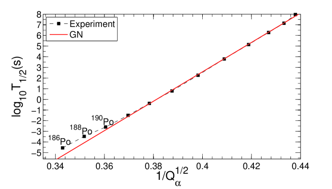
Figure 17: (Color online) The logarithms of the $\alpha$ decay half-lives of neutron-deficient Po isotopes as a function of $Q_{\alpha}^{-1/2}$.

For the polonium isotopic chain with $N<126$, as can be seen from Figs. 15 & 17, the linear behaviour of $log_{10}|R{\cal F}_{\alpha}(R)|^{2}$ breaks down below ¹⁹⁶Po. As a result, the Geiger-Nuttall law is broken in the light polonium isotopes. In ¹⁸⁶Po, the width difference between the experimental result and that predicted by the GN Law is as large as one order of magnitude [165]. This violation is induced by the strong suppression of the $\alpha$ formation probability due to the fact that the deformations (or shell-model configurations) of the ground states of the lightest $\alpha$-decaying neutron-deficient polonium isotopes ($A<196$) are very different from those of the daughter lead isotopes (see Sec. 5.8). One may say that the decay from ¹⁸⁶Po is strongly hindered that the “average” behaviour predicted by the GN law. On the other hand, we emphasize here that it is important to have an overall understanding of all alpha decay properties using UDL before one can draw conclusions on the enhancement or hindrance of the alpha formation probability of specific alpha decay processes. If one just look at the GN description of light Po isotopes, one may draw to the wrong conclusion that the alpha decay from light Po isotopes should be much hindered than heavier ones which, however, is not the case as can be seen from the figure. This is related to the fact that the generic behaviour of the alpha formation is washed out in the GN law description which is essentially a local theory with parameters fitted to each certain isotopic chain.

5.4.3 Generic form of the $\alpha$ formation probability

A generic form for the $\alpha$-particle formation amplitude as a function of nucleon (proton or neutron) number was proposed in Refs. [165, 166] based on experimental values [56] and calculations performed within the framework of the seniority scheme. This is shown in Fig. 18: When the nucleons are filling a new major closed shell (e.g. $N$ between 82 and 126) the $\alpha$-particle formation amplitude is nearly constant as high-$j$ orbitals are filled first. As soon as the low-$j$ orbitals are filled, the formation probability smoothly reduces until one reaches again a closed proton or neutron configuration, i.e. the upper boundary of the major shell. Here a minimum is reached. Crossing the closed shell induces a steep increase and the approximately constant trend mentioned above continues. However, when strong particle-hole excitations across closed shells are encountered, this ’generic’ form of the $\alpha$-particle formation probability is altered as one clearly sees in the light polonium isotopes. Such effects, however, do not invoke a disappearance of the influence of the $Z=82$ shell gap on the $\alpha$-decay probability.

Figure 18: A generic representation of the generic form of the evolution of the $\alpha$ formation probabilities $|RF(R)|^{2}$. Thick solid lines are for isotopes, where experimental data are available and dashed lines are extrapolations to the regions with the yet unavailable data. Taken from Ref. [166].

Guided by recent experimental findings, the $\alpha$-decaying nuclei was divided into four regions:
I) $N\leq 126$, $Z\leq 82$;
II) $N\leq 126$, $Z>82$;
III) $N>126$, $Z>82$;
IV) $N>126$, $Z\leq 82$.
Except for ²¹⁰Pb, $\alpha$ decay has not yet been observed for nuclei in region IV. The need for a different linear $Z$ dependence of the coefficients $A$ and $B$ of Eq. (25) in the four regions of the nuclear chart is obvious.

In comparison with those in region III for which the formation probabilities are nearly constant or only weakly depend on $Q_{\alpha}^{-1/2}$, the data in region II show an exponential dependence. The other isotopic chains in region II show a similar linearly decreasing behaviour of $log_{10}|RF(R)|^{2}$ as a function of $Q_{\alpha}^{-1/2}$, however, with different slopes. As a result, the GN law remains valid for isotopic chains in region II. However, the corresponding values of ${\cal A}$ and $|{\cal B}|$ will increase with $Z$ beyond the trend observed in regions I and III, as can be seen in Fig. 19. In regions I and III, Both ${\cal A}$ and $|{\cal B}|$ show a linear behaviour as a function of $Z$.

Approaching the $N=126$ shell closure with increasing neutron number, a strong and exponential decrease of the formation probability is observed. In spite of a variation of $|RF_{\alpha}(R)|^{2}$ over one order of magnitude, the GN law and the ${\cal A}$ and $|{\cal B}|$ linear dependence upon $Z$ are still valid. This has no real physical meaning, but is a consequence of the specific dependence of the $|RF_{\alpha}(R)|^{2}$ on $Q_{\alpha}$.

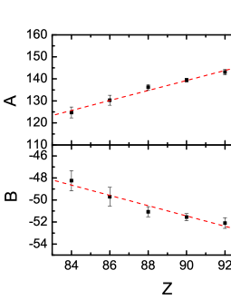
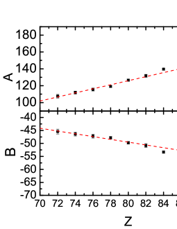
Figure 19: (Color online) The coefficients ${\cal A}$ and $|{\cal B}|$ of the GN law as a function of $Z$ for $\alpha$ decays in the Pb region corresponding to neutron numbers $N>126$(left, Region II) and $N<126$ (right, Region I& II).

5.5 $\alpha$ decays of $N\sim Z$ nuclei

One would expect that the influence of the neutron-proton (np) interaction upon alpha decay would be better taken into account in nuclei with the number of neutrons close to the number of protons. In such a case the shell model predicts that neutrons and protons move in the same shells and, therefore, the isovector monopole np interaction would not be hindered by constraints like parity restrictions. As we have seen, in heavy nuclei the neutron-neutron and proton-proton interaction, when treated properly, induce the nn and pp clustering [133]. Yet the decay width evaluated by including many configurations and even the proper continuum was too small. One may think that the reason of this failure is that the np interaction is not treated properly in the cases where the number of neutrons differs much from the number of protons. Therefore, the $\alpha$ decays from $N\sim Z$ nuclei can provide an ideal test ground for our understanding of the np correlations. This includes the isovector as well as the isoscalar pairing mode. The intense efforts to elucidate this problem can be attested by the long list of references, e. g. Refs. [168, 169, 170, 171, 172].

The many undertakings on the pn interaction in $N\sim Z$ nuclei and its effect upon $\alpha$-decay were hindered by the lack of experimental data. Finally an experiment was performed in which the isotopes ¹⁰⁹Xe and ¹⁰⁵Te were identified [173] through the detection of the $\alpha$-decay chain ${}^{109}Xe\rightarrow^{105}Te\rightarrow^{101}Sn$. The half-lives of the two $\alpha$-decays were determined to be $13\pm 2$ ms and $620\pm 70$ ns for ¹⁰⁹Xe and ¹⁰⁵Te, respectively. It was also found that the reduced $\alpha$-decay widths relative to ²¹²Po was enhanced in the two cases, which prompted the name of “superallowed $\alpha$-decay transitions”. This was aptly applied in this region of $N\sim Z$ where such a feature was expected. The authors of that experiment stated that and attempt to measure the $\alpha$-decay chain ${}^{108}Xe\rightarrow^{104}Te\rightarrow^{100}Sn$ were to be expected. This was indeed observed very recently in Ref. [174]. In addition, the $\alpha$ decays of ¹¹⁴Ba [175, 176] and light Xe and Te isotopes have also been observed [177, 178, 179]. An experimental search for ¹¹³Ba was presented recently in Ref. [180].

Figure 20: (Color online) $\alpha$-decay formation amplitudes $|RF_{\alpha}(R)|^{2}$ extracted from experimental data [56, 181] as a function $N$ for neutron-deficient Te (circle) and Xe (square) above ¹⁰⁰Sn. Open symbols correspond to the decays of $\alpha$ particles carrying orbital angular momentum $l=2$. The figure was taken from Ref. [182]. The new data on ¹⁰⁸Xe from Ref. [174] is added and highlighted in green.

In Fig. 20 is compared the $\alpha$ formation probabilities of nuclei just above ¹⁰⁰Sn. The $\alpha$ formation probabilities of those nuclei follows the general average mass-dependence trend of $\alpha$ formation probability systematics but shows rather large fluctuations and uncertainties. Contrary to what is stated in Ref. Ref. [174], it is still difficult to determine whether there is indeed an extra enhancement in those transitions. Further experimental investigation is essential in clarifying the issue. It may be useful to mention here that the systematics of formation probabilities for available $\alpha$ decays shows an increasing trend as the mass number decreases. This is related to the fact that the size of the nucleus also gets smaller, which favours the formation of $\alpha$ particles on the surface.

The robustness of the $N=Z=50$ shell closures has fundamental influence on our understanding of the structure of nuclei around the presumed doubly magic nucleus ¹⁰⁰Sn. It was argued that ¹⁰⁰Sn may be a soft core in analogy to the soft $N=Z=28$ core ⁵⁶Ni. It seems that such a possibility can be safely ruled out based on indirect information from recent measurements in this region [53, 183, 184, 185, 186]. It is still difficult to measure the single-particle states outside the ¹⁰⁰Sn core. The neutron single-particle states $d_{5/2}$ and $g_{7/2}$ orbitals in ¹⁰¹Sn, which have been expected to be close to each other, were observed by studying the $\alpha$-decay chain ¹⁰⁹Xe$\rightarrow$ ¹⁰⁵Te $\rightarrow$ ¹⁰¹Sn [173]. In Ref. [177], the nucleus ¹⁰⁵Te was also populated and one $\alpha$ transition was observed. A prompt 171.7 keV $\gamma$-ray transition was observed in Ref. [187] and was interpreted as the transition from the $g_{7/2}$ to the $d_{5/2}$ orbital, which was assumed to be the ground state. On the other hand, two $\alpha$ decay events from ¹⁰⁵Te were observed in Ref. [181] with the branching ratios (energies) of 89% (4711 keV) and 11% (4880 keV). Based on those observations and on the assumption that the ground state of ¹⁰⁵Te has spin-parity $5/2^{+}$, a flip between the $g_{7/2}$ and $d_{5/2}$ orbitals was suggested. This information was used in the optimization of the effective shell-model Hamiltonian for this region [188].

The influence of np correlation upon the formation of $\alpha$ particles in ²²⁰Ra and ^116,108Xe was studied in Ref. [189] within the framework of a generalized BCS approach in an axially deformed Woods-Saxon potential. Only diagonal terms between proton and neutron orbitals with the same angular-momentum projections were considered and a modest enhancement of the clustering was found in ^116,108Xe. In Ref. [172] the nn and pp two-body clustering in ¹⁰²Sn and ¹⁰²Te was analysed within the framework of the shell-model. The correlation angle between the clustered nucleons was investigated by switching on and off the np correlation . It was found that when a large number of configurations is included there is a significant enhancement of the four-body clustering at zero angle when the np interaction is switch on. This is an indication of the importance of the np interaction in the clustering process.

One would have expected an intense theoretical activity dealing with the superallowed $\alpha$-decay region. But this was not the case. In Ref. [190] an empirical Gamow inspired calculation was performed analysing $\alpha$-emitters close to the $N=Z$ line. As usual in this type of calculations the novel ingredient introduced as compared with previous like calculations was the $\alpha$-daughter interaction. Here a double folded potential was used. The calculations were found to be close to the experimental data. Also the half-lives of some of the neutron-deficient I, Cs, and Ba isotopes were predicted to be longer than 1 ms.

Another theoretical paper concerned with this region is Ref. [191]. Here the structure and the $\alpha$-formation probability corresponding to the nuclei ²¹²Po and ¹⁰⁴Te were studied using a full microscopic formalism within the shell-model. It was found that the proton-neutron correlations are much more important in $Te$ than in $Po$. This is expected, since the active neutrons and protons move in the same orbits in $Te$, but in different ones in $Po$. As a result the state ²¹²Po(gs) becomes a near pure monopole isovector state, while the state ¹⁰⁴Te(gs) presents strong mixing with other (multipole) states. Another consequence of the proton-neutron correlations is that the $\alpha$-particle formation probability in ¹⁰⁴Te is 4.85 times larger than that in ²¹²Po, thus attesting that in the Te region there is a superallowed $\alpha$-decay transition. Yet the $\alpha$-decay width is too small as compared with the expected experimental value. This is another strong indication that the standard shell model representation needs some additional ingredient. On the other hand, the proton-neutron BCS calculations presented recently in Ref. [192] tend to argue that the proton-neutron pairing correlations have a small influence on the alpha particle formation in $N=Z$ nuclei above ¹⁰⁰Sn.

5.6 BCS treatment of alpha decay and pairing correlation

The BCS approach was introduced just in the beginning of the microscopic studies of $\alpha$-decay [127, 193, 194, 195]. The great appealing of this approach resides in its ability to transform the wave function of a correlated system into a pure quasiparticle configuration. This is a consequence of the dominant isovector pairing force in nuclei. A many-nucleon superconducting nucleus is controlled by very few quasiparticle degrees of freedom. This made it possible to evaluate nuclei with nucleon number lying between magic numbers even with limited computing facilities, as those available five decades ago. An early and detailed calculation of decay widths using this formalism was presented in Ref. [196]. Hundreds of transitions were calculated and the empirical trends were well reproduced.

The isovector pairing correlation is behind the success of the BCS theory in nuclei. As already mentioned above, this correlation manifests itself through the coherent contribution of a large number of shell-model configurations. The isovector pairing correlation highly enhances the calculated $\alpha$-decay width and is indeed the mechanism governing the formation of $\alpha$ particles at the nuclear surface. This feature is also responsible for the two-particle clustering, which is manifested in a strong increase in the form factor of the two-particle transfer cross section in transfer reactions between collective pairing states. As we have seen, this also gives rise to giant pairing resonances, which correspond to the most collective of the isovector pairing states.

Figure 21: (color online). Upper panel: $\alpha$-particle formation probabilities for the decays of the even-even isotopes as a function of the neutron numbers $N$ of the mother nuclei. Lower panel: Neutron pairing gaps in even-even lead to Thorium nuclei extracted from experimental binding energies. From Ref. [165].

Fig. 21a shows the formation probabilities $|RF_{\alpha}(R)|^{2}$ extracted from the experimental half-lives from known ground state to ground state $\alpha$-decay transitions in even-even isotopes from $N=92$ to 140. From the trend of $|R{\cal F}_{\alpha}(R)|^{2}$ around the neutron shell closure at $N=126$, one can deduce a global trend. Below the shell closure, $|R{\cal F}_{\alpha}(R)|^{2}$ decreases as a function of rising neutron number, reaching its lowest values at the shell closure. When the shell closure is crossed, a sudden increase in $|R{\cal F}_{\alpha}(R)|^{2}$ is observed. It is followed by an additional but smaller increase and finally saturation occurs. The $\alpha$-particle formation amplitudes for nuclei ¹⁶²W, ¹⁶²Hf [197] and ¹⁹³At [198] are systematically larger than those of neighbouring nuclei, which is not understood and needs further investigation.

Within the BCS approach the two-particle formation amplitude is proportional to $\sum_{k}u_{k}v_{k}$ where $u_{k}$ and $v_{k}$ are the standard occupation numbers. To this one has to add the overlaps of the corresponding proton and neutron radial functions with the $\alpha$-particle wave function on the nuclear surface, which do not differ strongly from each other for neighbouring nuclei. The BCS pairing gap is given by $\Delta=G\sum_{k}u_{k}v_{k}$, where $G$ is the pairing strength. It indicates that the $\alpha$ formation amplitude is proportional to the product of the proton and the neutron pairing gaps which can serve as a signature of the change in clusterization as a function of the nucleon numbers. To probe this conjecture one may compare the formation probabilities extracted from the experimental half-lives to the corresponding pairing gaps. The latter can readily be obtained from the experimental binding energies as [165, 199, 135, 200, 201, 200, 202]

$$\Delta_{n}(Z,N)=\frac{1}{2}\left[B(Z,N)+B(Z,N-2)-2B(Z,N-1)\right].$$ (30)

The empirical pairing gaps are shown as a function of the neutron number in Fig. 21b. One indeed sees a striking similarity between the tendency of the pairing gaps in this figure with the $\alpha$-particle formation probabilities. This similarity makes it possible to draw conclusions on the tendencies of the formation probabilities. The near constant value of $|R{\cal F}_{\alpha}(R)|^{2}$ for neutron numbers $N\leq 114$ is due to the influence of the $i_{13/2}$ and other high-$j$ orbitals. As these highly degenerate shells are being filled the pairing gap and the formation probability should remain constant, as indeed they do in Fig. 21. A quite sharp decrease of formation probability and pairing gap happens as soon as the low-$j$ orbitals like $2p_{3/2}$, $1f_{7/2}$ and $2p_{1/2}$ start to be filled. Finally, when we reach $N=126$, the pairing gap reaches its lowest value. The possible influence of the $Z=82$ shell closure on the $\alpha$ formation probability and the robustness of the shell was also discussed in Ref. [165], which was questioned based on earlier measurements on the $\alpha$ decays of neutron-deficient Pb isotopes [203].

The role of the pairing interaction in multi-quasiparticle isomeric states and the reduction of pairing in those states on $\alpha$-decay half-lives was examined in Ref. [204].

Primary time-dependent Hartree-Fock calculations for $\alpha$ decay and $\alpha$ capture were already carried out in Ref. [205] with a simplified Skyrme plus Yukawa potential. No spin-orbital field was considered in that paper. Significant progress has been made in the development of nuclear energy density functional approaches which are now able to provide a reasonable description of ground state binding energies and densities throughout the nuclear chart, even though the description of the single-particle spectroscopy is still less satisfactory. The Skyrme-Hartree-Fock single-particle wave functions were applied to calculate the $\alpha$ formation amplitudes in even-even nuclei in Refs. [206, 207] and even-odd nuclei [208]. However, the calculated formation amplitude is still several of orders of magnitude too small in comparison to experimental data. The application of the recently refined functional seems to make the discrepancy even worse [207]. Further investigation along this line would be interesting to understand the origin of the discrepancy, which may shed additional light on the constraint of the density functional.

5.7 Nuclear deformation and $\alpha$-decay

The treatment of $\alpha$-decay processes from deformed nuclei began soon after Bohr and Mottelson proposed the rotational model [209]. In contrast to the case of spherical nuclei the WKB approximation as used by Gamow [3] and most other calculations of alpha decay since then, cannot be applied. This is because only when there is no interference between two degrees of freedom one can perform the integration on one variable independently of the other. Instead, in the case of deformed potentials the Hamiltonian includes terms where the radial and angular variables interfere with each other. This difficulty was overcome by generalizating the WKB approximation to deformed systems, as done by Bohr and Mottelson [210] and described in detail in Ref. [211]. In this theory the formation amplitude enters in a more complicated fashion than in the Thomas formulation described above. For a comprehensive presentation of the theory and its application see Ref. [12]. This method was used extensively [196, 209, 129, 212], in particular to describe anisotropy in $\alpha$-decay [213, 214, 215, 216, 217].

The exact treatment of the $\alpha$-decay process in deformed nuclei requires a coupled channel (CC) approach. A CC as well as a WKB calculation of the decay width in the transition ¹⁵²Dy $\rightarrow\alpha$+¹⁴⁸ Gd was performed in Ref. [218]. As seen in Table I of this reference the WKB width coincides with the exact one for small deformations, but already for $\beta$=0.3 the WKB width, $\Gamma_{WKB}$, is nearly double the exact one, $\Gamma_{cc}$. For $\beta$=0.8 it is $\Gamma_{WKB}/\Gamma_{cc}$=65.3. This is a drawback which, together with the difficulties of the method, prompted the proposal of other approaches, like the one in Refs. [219, 220, 221] where, in addition, a critical assessment of the WKB approximation is presented.

The coupled-channel approach provides a microscopic foundation to study the multi-dimensional decay and reaction processes. Usually, the wave function is propagated numerically starting with proper initial conditions. The coupled-channel equations can be written in matrix notation as

$$\Psi^{\prime\prime}(r)=\left[\frac{2\mu}{\hbar^{2}}V(r)-k^{2}I\right]\Psi(r).$$ (31)

Here $V(r)$ denotes the potential matrix with the dimension $N$. The radial wave function $\Psi(r)$ is a $N\times N$ square matrix with each column being a linearly independent solution of the equations. Usually the wave functions are propagated starting with $N$ initial conditions (through, e.g., the Numerov procedure). However, this propagation is numerically quite unstable since at the classically forbidden region the propagation of the corresponding exponentially growing components destroys the independence of the solutions.

Instead, one can propagate the set of coupled equations for the logarithmic derivative $Y(r)=\Psi^{\prime}(r)\Psi(r)^{-1}$,

$$Y^{\prime}(r)=\left[\frac{2\mu}{\hbar^{2}}V(r)-k^{2}I\right]-Y^{2}(r).$$ (32)

The log derivative matrix in above Ricatti-type equation can be propagated directly without the stability problem met in the integration of the coupled-channel equation. We have developed an invariant embedding procedure to solve above log-derivative equation. In the CC formulation one expands the deformed wave function in terms of its spherical components $g_{c}$, where the index $c$ labels the quantum numbers of the spherical wave, including the angular momentum $l$. Therefore the asymptotic form of these radial components is as in the spherical case, i. e.,

$$\lim_{r\rightarrow\infty}g_{c}(r)=N_{c}H^{(+)}_{l}(\chi,K_{c}r)$$ (33)

where, as in the spherical case, $\chi$ and $K_{c}$ are the Coulomb parameter and the wave number, respectively. Also as in the spherical case, the constant $N_{c}$ is obtained by matching the external and internal wave functions. A detailed presentation of the CC method can be found in Ref. [222].

In spite of the shortcomings of the WKB approach it was found that a simplification of its formulation provides decay widths which are very close to the coupled-channel values in the laboratory frame [223]. This has an influence in recent developments in modern laser facilities. Such facilities will allow one to probe nuclear properties by using strong electromagnetic fields [224, 225]. This prompted an intense research activity trying to find means to exploit these facilities in the pursue of yet unknown nuclear features. The most relevant of these inquiries so far is the study of the nuclear behaviour under strong laser fields. Those studies use the modified WKB approximation of Ref. [223]. Thus, in Ref. [226] it is found the remarkable property that as a consequence of the laser field the penetrability of the $\alpha$-particle through the Coulomb barrier may be reduced by many orders of magnitude. Due to this property one may treat nuclear wastes in dedicated facilities by exposing them to strong laser fields. The resulting decay of alpha particles through the weak Coulomb barrier would transform the dangerous isotopes contained in the waste into lighter short living nuclei, thus eliminating one of the major hinders in the use of nuclear power. This conclusion was confirmed by an independent study [227]. Moreover, in another recent publication it is shown that besides alpha-decay proton- and cluster-emission may be important modes of decay under strong magnetic fields and, therefore, as a means of reducing nuclear wastes [228]. In this paper it is even found that proton-decay may become the main form of decay even when normally alpha-decay would be dominant. This is an important point which may trigger new inquiries in the old subject of radioactive particle decay.

5.8 Alpha decay as a probe to nuclear shape changes and shape coexistence

The $\alpha$ decays from ground states to excited states (fine structure) as well as the decays from excited states are usually less favoured than ground-state to ground-state decays. Already in the beginning of microscopic studies of $\alpha$-decay the concept of reduced width, and the ratio between reduced widths for transitions to ground and excited states, was introduced to estimate the strength of a transition [229]. The usefulness of these early notions can be pondered by their importance and use even today, as e. g. in Ref. [34],

Similar early studies were performed in relation to transitions to vibrational states [230] and, more recently, in [231, 232, 233]. There have also been a large amount of work dealing with transitions to and from rotational states [196, 234, 235, 236]. A recent review on the application of the coupled channel approach to the $\alpha$ decay fine structure can be found in Ref. [237].

Usually the ground state to ground state (gs to gs) alpha-decay transitions in even-even nuclei are much more probable than the corresponding transitions to excited states. This feature depends strongly upon the Q-value, i. e. upon the penetrability of the alpha-particle. The Q-value contains no information on the structure of the nuclei involved in the transition, like pairing collectivity. This information pertains to the formation probability, as we have seen in Subsection 5.2. To extract information about the characteristics of the nuclei connected by the $\alpha$-decay process a quantity called ”hindrance factor” (HF) was defined in Ref. [238]. The HF is the ratio of the formation probabilities corresponding to the gs to gs divided by the gs to excited state transitions. In that reference the HF were evaluated microscopically without including continuum configurations. Yet the results agree well with the corresponding experimental data. One may argue that this good agreement is because the continuum affects equally all states. Therefore in the ratio of the HF the contribution of the continuum is cancelled. However, that is not the case in the calculations of Ref. [231] where absolute transitions were studied without including the continuum either. Yet the results also agree well with experiment. One therefore concludes that the shortcomings of the shell model mentioned in Subsection 5.2 affects only $0^{+}_{1}$ collective pairing states.

Systematic evaluations of the $\alpha$-decay fine structure were also done recently in Refs. [239, 240]. It was found that the $\alpha$ decays to excited states also follow the Viola-Seaborg law discussed above (see Eq. (26)).

The $\alpha$ decay transitions of neutron-deficient nuclei around $Z=82$ are of particular interest because through such transitions one can uncover features like the co-existence of states with different shapes [241]. Thus, three low-lying $0^{+}$ states in ¹⁸⁶Pb were observed following the $\alpha$ decay of ¹⁹⁰Po(gs) [242]. These three states have been found to be of quite different shapes, namely spherical, oblate and prolate. The transition ¹⁸⁷Po(gs)$\rightarrow\alpha$+¹⁸³Pb(gs), where ¹⁸³Pb(gs) is spherical, was observed to be strongly hindered [243] whereas the decay to a low-lying excited state at 286 keV was favoured. Based upon a potential energy surface calculations, the ¹⁸⁷Po ground state and the 286 keV excited state in ¹⁸³Pb were interpreted as of prolate shape. The decay to the ¹⁸³Pb ground state is hindered since this state has a spherical shape which is different from that of the ground state. The difference in the shapes indicates that the configurations of the mother and daughter nuclear wave functions are very different. As a result, the $\alpha$ formation amplitude is significantly reduced.

In another experiment the HF corresponding to the $\alpha$ decay of the isomeric state in ¹⁹¹Po was shown to have the same origin, i. e. the mother and daughter nuclei have different shapes [244]. The HF corresponding to the $\alpha$ decays of neutron-deficient even-even nuclei around $Z=82$ was measured in Ref. [245]. The $\alpha$ decays to and from the excited $0^{+}_{2}$ states in Po, Hg and Rn isotopes were studied in Refs. [238, 246, 247]. These states are described as the minima in the potential energy surface provided by the standard deformed Woods-Saxon potential. A simple approach was also presented in Ref. [248] to evaluate the HF by taking the ratio between the wave function amplitudes for the transitions to the ground and excited $0^{+}$ states of the daughter nucleus obtained from potential energy surface calculations.

In a recent experiment, the fine structure has been observed in the $\alpha$ decay of the high spin isomeric states in nuclei ¹⁵⁵ Lu($25/2^{-}$) and ¹⁵⁶Hf($8^{+}$) [249]. A significantly strong hindrance is seen for the decay to the seniority $v=3$ and 2 states in the corresponding daughter nuclei. These lighter nuclei can be evaluated within the framework of large-scale shell model [250]. The main configuration of the $25/2^{-}$ isomer in ¹⁵⁵ Lu has been assigned as $\pi(h_{11/2})^{3}\otimes\nu f_{7/2}h_{9/2}$. The decay of such a configuration to the ground state ($11/2^{-}$) of ¹⁵¹Tm is hindered by a factor of nearly 20 in comparison with the g.s. to g.s. transition in relation to the broken neutron pair in the decay state. The decay to other $v=3$ states is hindered by factors upto 300.

In conclusion of this Subsection, the study of fine structure in nuclei has shed new light on nuclear structure studies. It has provided a decisive evidence of shape coexistence in nuclei and, also very important, has shown that the shell model representation is able to properly describe $\alpha$-decay transitions in nuclei.

6 Heavy cluster decay

In 1977 W. Greiner and A. Sandulescu analysed in detail the mass and charge distributions of fission fragments as a function of the positions of the fragmentation valleys [251]. They found that asymmetric shapes are generated mainly by the minima in the potential and that there might occur a new and highly asymmetric fission in which one of the fragments is close to the double magic nucleus ²⁰⁸Pb. This would correspond to a new form of spontaneous particle emission where the decaying particle would be much heaver than ⁴He.

And indeed this spontaneous emission of clusters heavier than the $\alpha$ particle was observed seven years later from a systematic study of the properties of nuclei heavier than lead [252]. The decaying cluster was identify as the nucleus ¹⁴C. It was observed in competition with $\alpha$-decay from the mother nucleus ²²³Ra leaving behind the daughter nucleus ²⁰⁹Pb, as predicted in Ref. [251]. The branching ratio for emission of ¹⁴C relative to $\alpha$-particles was about $10^{-9}$. The corresponding relative decay widths was measured to be $\Gamma(^{14}C)/\Gamma(\alpha)=(6.1\pm 1.0)\times 10^{-10}$ [253, 254]. This was an outstanding experimental feat and was claimed as the greatest achievement in radioactive decay since Becquerel [255]. Since then the emission of heavier clusters including ²⁰O, ²³F,^22-26Ne, ^28,30Mg, and ^32,34Si have been observed.

Many calculations were done soon afterwards trying to understand the mechanisms that induce the decay of heavy clusters as well as to explore the possibility of finding by-products of the decay process. Thus, a calculation performed by using Eq. (3) for the decay width from ²²²Ra showed that the relative formation probability of ¹²C with respect to the formation of $\alpha$-clusters is $|{\cal F}(^{12}C/{\cal F}(\alpha)|^{2}=3.3\times 10^{-3}$ [256]. It was also found that this ratio diminishes strongly with the size of the cluster. For example, in the decay ${}^{216}Rn\rightarrow^{8}Be+^{208}Pb$ it is $\Gamma(^{8}Be)/\Gamma(\alpha)=3.8\times 10^{-15}$, $|{\cal F}(^{8}Be/{\cal F}(\alpha)|^{2}=5.7\times 10^{-3}$, while for the decay ${}^{247}Bk\rightarrow^{46}Ar+^{201}Au$ it is $\Gamma(^{46}Ar)/\Gamma(\alpha)=6.6\times 10^{-19}$ and $|{\cal F}(^{46}Ar/{\cal F}(\alpha)|^{2}=3.0\times 10^{-9}$.

Microscopic calculations as those performed in $\alpha$-decay have not been possible in the case of heavy cluster-decay. There was an attempt to evaluate the emission of ¹⁴C from $Ra$ isotopes [257]. In order to make the calculation feasible crude approximations had to be applied. As a result the evaluated quantities disagreed greatly from experiment and no attempt to perform such calculations was attempted afterwards. Thereafter the calculations were done within effective frameworks, as those discussed in the previous Section.

The fission-like approach of cluster decay which, as discussed above, is at the origin of cluster decay processes, has been very successful in describing cluster decay. There are many works performed within this framework. The most recent ones are in [258, 259, 260]. In the references therein one can find the developments in this subject during the last years. In this context it is important to underline that a recent and important example which uses the Gamow approach is in [261]. The importance of this paper is that it shows that in superheavy nuclei the dominant decay mode is $\alpha$-decay, in contradiction of the fission-like study of cluster decay performed in Ref. [262].

Cluster states in nuclei were investigated since a long time [263]. One of these investigations had an impact in future studies of cluster decay [264]. The model proposed in this reference was first applied in $\alpha$-decay [265] and then in clusterization in general [266] and references therein.

6.1 Description of the cluster decay with generalized GN law

There have been a number of papers dealing with generalizations of the Geiger-Nuttall law which includes cluster decay. One advantage of these generalizations is that if reliable values of decay $Q$ values can be obtained, it is easy to extrapolate to all kinds of cluster decays throughout the nuclear chart. Systematic calculations of the decays of clusters heavier than ⁴He were done in Refs. [160, 162, 164, 267]. In particular, as mentioned before, the UDL works well for all proton, alpha and heavy cluster decays. This is because the cluster formation probability, as shown in Fig. 22, follows roughly a linear behaviour as a function of $\rho^{\prime}$. Therefore, all those decays can be described consistently within the same framework. Such calculations were extrapolated to the decays of even heavier clusters from superheavy nuclei to daughter nuclei around ²⁰⁸Pb in Ref. [262] and later in Refs. [268, 269]. Although these efforts have been very fruitful there are uncertainties behind the extrapolation which requires further analysis. This is an open task.

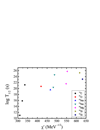
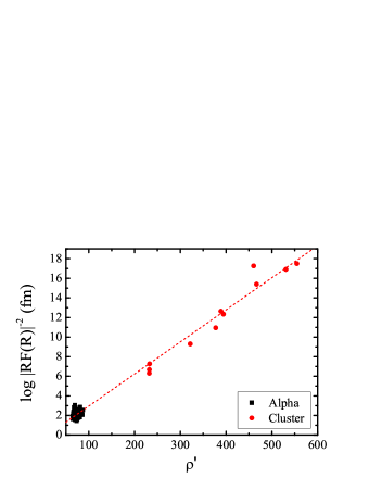
Figure 22: Upper: Systematics of cluster decay half-lives for even-even nuclei as function of $\chi^{\prime}$. Lower left: The heavy cluster decay formation probabilities $\log|RF(R)|^{-2}$ as a function of the charge number of the mother nucleus $Z$. Lower right: The formation probabilities $\log|RF(R)|^{-2}$ for both $\alpha$ and heavy cluster decays as a function of $\rho^{\prime}$. Taken from Ref. [160].

There are a plethora of effective calculations of cluster decay performed within the framework of the Gamow theory. We will here mention a few, although the interested reader can also consult the references therein, corresponding to the latest years. In Ref. [267] the width is evaluated by using Eq. (34) with $F_{{\rm eff}}=P_{c}F_{c}$, where $P_{c}$ is the preformation factor of the cluster $c$ in the mother nucleus and $F_{c}$ is obtained through the so-called normalization factor, leading to Eq. (14) of that reference. This is actually based in Eq. (15) of Ref. [270]. Essentially what is done is to use an effective cluster-nucleus interaction which can be obtained using the double folding model. For example, in Ref. [271], it is obtained from the double folding integral of the renormalized $M3Y$ nucleon-nucleon interaction and of the density distributions of the $\alpha$- particle and daughter nucleus. The model reproduces fairly well the half lives corresponding to the decays of clusters in the region $(^{14}C-^{34}Si$).

Another similar but much more simpler example is to take $F_{{\rm eff}}=\nu P_{c}$, where $\nu$ is the Gamow ”assault frequency” and $P_{c}$ is, as above, the preformation probability. This very traditional and simple Gamow approach gives, by using suitable values of the parameters, a reasonable account of the half lives of 26 experimentally known cluster decay half lives.

We notice that a quite common practice is to extract or define the effective cluster preformation factor empirically based on the discrepancy between the calculated and experimental half-lives of the cluster emitters.

In the same fashion as trans-lead nuclei decay into daughters around the doubly magic nucleus ²⁰⁸Pb, a second island of cluster radioactivities is expected in trans-tin nuclei decaying into daughters close to ¹⁰⁰Sn (see, for example, Ref. [160]). Such studies can be easily done within the generalization of the Geiger-Nuttall law to cluster decays. In particular, there have been tremendous efforts trying to detect the possible ¹²C emission from ¹¹⁴Ba [272, 273] and even ¹¹²Ba but so far there has been no success. That decay process from ¹¹⁴Ba was calculated in Ref. [274] with different models.

7 Effective approaches

The great success of the Gamow theory can be measured by its wide acceptance even today. In this theory, and many other similar ones, the decaying $\alpha$ particle is assumed to be a preformed particle which is trapped inside the mother nucleus by the nuclear, Coulomb and centrifugal potential. It is assumed that this particle has no intrinsic structure and that the decay width $\Gamma$ is just proportional to the penetrability, i. e.

$$\Gamma=F_{{\rm eff}}\exp\left[-2\int^{R_{2}}_{R_{1}}k(r)dr\right],$$ (34)

where $F_{{\rm eff}}$ is an unknown quantity that is taken as a free parameter to be fitted to experimental data. Different authors give different interpretations to this quantity. In the first effective theory of alpha-decay [3] Gamow introduced the concept of hitting frequency. That is, he assumed that the $\alpha$-particle moves freely inside the mother nucleus. It would escape the nuclear and Coulomb barriers when hitting the wall of the nucleus from inside. The hitting frequency, i. e. the coefficient $F_{{\rm eff}}$, is given by $F_{{\rm eff}}=v/R$, where $R$ is the nuclear radius and $v$ the velocity of the $\alpha$-particle. This, and the wave number $k$ in the equation above, are given by $v=\sqrt{2Q_{\alpha}/\mu}$ and $k(r)=\sqrt{2\mu|Q_{\alpha}-V(r)|}/\hbar$ where $\mu$ is the effective mass and $V(r)$ the effective potential between the cluster and the daughter nucleus, including the Coulomb field. The radii $R_{1}$ and $R_{2}$ are turning points, i. e. the points $r$ that satisfies $V(r)=Q_{\alpha}$.

A different kind of effective model was proposed in Ref. [275], where the $\alpha$-cluster is assumed to be an inert particle moving in orbits with large values of a global quantum number. This alpha-cluster model was actually proposed long before [276]. In this paper it was found that an $\alpha$-cluster model with parameters values which optimize the fit to $\alpha$-decay lifetimes for a wide range of nuclei, results in good agreement with the $\alpha$-and $\gamma$-decay properties of states belonging to the ground state band of ²¹²Po. The reliability of this model was strengthened by the work in Ref. [275], where the $\alpha$-particle-core potential is taken to be of squared-well form, with fixed depth, and radius given by the Bohr-Sommerfeld condition. This rather simple model reproduces well all the $\alpha$-decay half-lives for heavy even-even nuclei. This result can be considered farther evidence that the wave functions dealing with alpha-decay has to include cluster components, as discussed above.

In spite of the accurate results of this model its use is difficult in comparison with the effective procedures based upon the Gamow model, where the calculations can be performed by using a simple pocket calculator and its predictive power is good enough to guide experimental searches. That is the reason why variations of the Gamow model are mostly used when dealing with alpha-decay studies. One sees that in the simple and outstanding Gamow theory there is only one free parameter, namely the nuclear radius $R$, which is well determined within less than an order of magnitude. In radioactive decay studies this is a rather small error. And even more impressive is that only the inverse of $R$ (and not the exponential) enters in Eq. (34). Instead, the exponential is very sensitive to $R_{1}$ and $R_{2}$, but that is the usual limitation of the WKB approximation. The problem with this beautiful theory is that it is too simple and that it violates crudely the Pauli principle, although when the theory was presented this was compensated by the great breakthrough introduction of the concept of quantum penetrability,

Similar empirical approaches, even for cluster decays, were developed through the years. Most of these applications consist of various versions of the nuclear potential in Eq. (34). This is odd since one expects that the value of the short range nuclear potential should be negligible in the integration range, i. e. between $R_{1}$ and $R_{2}$, in Eq. (34). In this context it is worthwhile to point out that this nearly independence upon the nuclear potential in $\alpha$-decay effective theories is not shared by the exact treatment of the Thomas decay width [10]. Here the internal wave function ${\cal F}_{c}(R)$ is mainly determined by the nuclear interaction, although the Coulomb part plays also a role.

In spite of this weak dependence upon the nuclear interaction, different effective theories provide different values of the width. We will not go into these details for all the large number of effective $\alpha$-decay models introduced in the past. Instead we will refer to some of the recent publications, and references therein, on this subject. Thus, in Refs. [190, 277, 278, 279, 280, 281, 282, 283] the width is evaluated according to Eq. (34) with different potentials and different values of $F_{{\rm eff}}$. Among these theories we will briefly describe, as a typical example, the one in Ref. [284] which is valid for all sort of clusters, including $\alpha$-clusters.

The nuclear-cluster potential is approximated by the relation

$$V_{N}(r)=\lambda(N_{c}v_{n}(r)+Z_{c}v_{p}(r))$$ (35)

where $\lambda$ is a folding factor, $N_{c}$ and $Z_{c}$ are neutron and proton numbers in the cluster, $v_{n}(r)$ and $v_{p}(r)$ are single neutron and proton fields (excluding the Coulomb potential). For the single-particle potentials a square well form was adopted. The folding factor $\lambda$ was determined by using the Bohr-Sommerfeld condition with the Wildermuth rule as,

$$\int_{0}^{R_{1}}\sqrt{\frac{2\mu}{\hbar^{2}}[Q_{\alpha}-V(r)]}\text{d}r=(G+1)\frac{\pi}{2}=(2N+L+1)\frac{\pi}{2},$$ (36)

where $G$ is the global quantum number and $N$ the number of nodes. $R_{1}$, $R_{2}$ and $R_{3}$ below are turning points obtained by $V(r)=Q_{\alpha}$.

There is no microscopic approach to define a unique value for the quantum number $G$. Since it is expected that the $\alpha$ cluster should be built upon valence nucleons occupying orbits just above the Fermi surface, the value of quantum number $G$ is usually taken from the Wildermuth rule as,

$$G=(2N+L)=\sum_{i=1}^{4}(2n_{i}+l_{i})=\sum_{i=1}^{4}g_{i}.$$ (37)

$g$, $n$ and $l$ are corresponding quantum numbers of the nucleons in the $\alpha$ cluster. The decay width is given as

$$\Gamma=F\frac{\hbar^{2}}{4\mu}\text{exp}\left[-2\int_{R_{1}}^{R_{2}}drk(r)\right],$$ (38)

where $k(r)$ the wave number,

$$k(r)=\sqrt{\frac{2\mu}{\hbar^{2}}|V(r)-Q_{\alpha}|}.$$ (39)

$F$ is the normalization factor determined by

$$F\int_{0}^{R_{1}}dr\frac{1}{k(r)}\cos^{2}\left[\int_{0}^{r}dr^{\prime}k(r^{\prime})-\frac{\pi}{4}\right]=1.$$ (40)

The decay width is as in Eq. (34) with $F_{{\rm eff}}=PF$ where $P$ is the cluster preformation probability and the normalization factor F is determined by a normalization condition. The preformation probability was assumed to be $P=1$. This and the normalization condition were also taken from [275]. Notably, this simple method reproduces the widths of a large number of alpha-decay data within a factor of about 2.

An effective $\alpha$-particle decay equation was derived for the $\alpha$ particle on top of the ²⁰⁸Pb core in Refs. [285, 286], where an attractive pocket-like potential appears around the nuclear surface. That is related to the sharp disappearance of the nucleon density in the Thomas-Fermi model employed in those works. Using the separation point $r_{sep}$ between the $\alpha$-particle and the daughter nucleus at the rather large distance of $r_{sep}$= 15 fm good agreement with experiment is obtained.

An effective method which does not rely upon the Gamow theory was developed in the 1970s. This formalism treats radioactive decay as an extension of the one corresponding to nuclear fission [251]. This is not surprising, since decay and fission are similar processes which are determined by the Coulomb and centrifugal barriers. This method had some success in predicting alpha-decay processes, but its great breakthrough occurs when it predicted cluster decays which were later confirmed experimentally, as seen in the next Section.

In spite of its shortcomings effective theories have been very successful in evaluating with reasonable accuracy and in a very simple and fast fashion $\alpha$- and cluster decay widths.

7.1 The cluster formation probability versus the preformation factor

The cluster formation probability $|F_{c}(R)|^{2}$ (or the formation amplitude $F_{c}(R)$) can be extracted from the experimental half-lives data and is a model-independent quantity. As shown above, in practice we also often use the quantity $|RF_{c}(R)|^{2}$ indiscriminately as the formation probability since it is easier to extract from data. On the other hand, the so-called preformation factor, given as the difference between the calculation and the experimental datum, is often introduced in many effective models. This preformation factor depends strongly on the shape of the effective potential employed [275]. Particularly, it is not a physical quantity that can be calculated microscopically. The reduced width introduced in Ref. [287] is also a similar effective quantity that depends on the effective optical potential. We suggest that it is the formation amplitude or formation probability that should be calculated and compared with those extracted from experimental data. On the other hand, the barrier penetration probability has been well understood since 1920s and contains on information on the nuclear structure property. Another model independent quantity is the ratio $N_{0}\equiv RF(R)/H_{0}^{+}(\chi,\rho)$ which can also be extracted from the experimental data.

The classical expression for the decay width $\Gamma_{c}$ (Eq. (1)) can be rewritten written as

$$\Gamma_{c}=\hbar\nu\left|\frac{R{\cal F}_{c}(R)}{H_{l}^{+}(\chi,\rho)}\right|^{2}=2P_{l}(R)\frac{\hbar^{2}}{2\mu R}|{\cal F}_{c}(R)|^{2},$$ (41)

where $l$ is the angular momentum carried by the outgoing $\alpha$-particle, ${P}$ is the penetration probability. The combination of regular and irregular Coulomb functions $F$ and $G$ is proportional to the Hankel function $H^{+}$. The quantities $\rho$ and $\chi$ are $\rho=\mu\nu R/\hbar$ and $\chi=2Z_{c}Z_{d}e^{2}/\hbar\nu$. $\mu$ is the reduced mass and $Z_{d}$ is the charge number of the daughter nucleus. $R$ should be chosen that the nuclear potential has vanishing value and the cluster and the daughter nucleus has already been fragmented. Although we have discussed it already, it is convenient for the presentation to emphasize that the quantity ${\cal F}_{c}(R)$ is the formation amplitude of the cluster at distance $R$ where only the Coulomb interaction is relevant. At this point the internal wave function ${\cal F}_{c}(R)$ is matched with the wave function of the outgoing particle. The decay width is independent upon $R$, which implies that the strongly R-dependent Hankel function is balanced by the equally strongly dependent formation amplitude.

Here we show how the two-step mechanism is manifested in effective models that the formation process is not explicitly taken into account. In the semiclassical approach, the decay width is given as

$$\Gamma=S_{{\rm eff}}F_{{\rm eff}}\exp\left[-2\int^{R_{2}}_{R_{1}}k(r)dr\right],$$ (42)

where $S_{{\rm eff}}$ is the effective preformation factor, $F_{{\rm eff}}$ a proper normalization factor [275] and $R_{1}$ and $R_{2}$ the classical turning points. Since the radius $R$ should satisfy the relation of $R_{1}<R<R_{2}$, we have

$$\Gamma=S_{{\rm eff}}F_{{\rm eff}}\exp\left[-2\int^{R}_{R_{1}}k(r)dr\right]P(R),$$ (43)

where $k(r)=\sqrt{2\mu|Q_{c}-V(r)|}/\hbar$ with $V(r)$ being the effective potential between the cluster and the daughter nucleus. The integration from $R_{1}$ to $R$ mimics the cluster formation probability in an effective way. For convenience we have defined a penetration factor $P$ that is given as

$$P(R)=\exp\left\{-2\int^{R_{2}}_{R}\sqrt{\frac{2\mu}{\hbar^{2}}|V_{{\rm C}}(r)-Q_{c}|}dr\right\},$$ (44)

where $V_{{\rm C}}(r)=Z_{d}Z_{c}e^{2}/r$ is the Coulomb potential. Above equation can be integrated exactly, giving,

$$P = \exp\left\{-2Z_{c}Z_{d}e^{2}\sqrt{\frac{2\mu}{Q_{c}\hbar^{2}}}\right.\left.\left[\arccos\sqrt{\frac{R}{R_{2}}}-\sqrt{\frac{R}{R_{2}}}\sqrt{1-\frac{R}{R_{2}}}\right]\right\}.$$

Inserting $\chi=Z_{c}Z_{d}e^{2}\hbar\sqrt{{2\mu}/{Q_{c}}}$, $R_{2}=Z_{c}Z_{d}e^{2}/Q_{c}$ and

$$\frac{R}{R_{2}}=\frac{\rho}{\chi}=\frac{Q_{c}}{V_{{\rm C}}(R)},$$ (45)

one immediately recognized that the penetration factor in the effective approach is related to the Coulomb function as,

$$P=\frac{[H^{+}_{0}(\chi,\rho)]^{-2}}{\tan\beta}=\exp\left[-2\chi(\beta-\sin\beta\cos\beta)\right].$$ (46)

Similarly, the decay width in the fission model can be given as [288],

$$\Gamma = F_{{\rm f}}\exp\left[\frac{-2}{\hbar}\int^{R_{2}}_{R_{f}}\sqrt{2B(r)E(r)}dr\right]$$ (47)

$$= F_{{\rm f}}\exp\left[\frac{-2}{\hbar}\int^{R}_{R_{f}}\sqrt{2B(r)E(r)}dr\right]P(R),$$

where $F_{{\rm f}}$ is the frequency of assaults, $B(r)$ the nuclear inertia, $E(r)$ the deformation energy from which the $Q$ value has been subtracted. The relation above holds because one should have $B(r)=\mu$ and $E(r)=V_{{\rm C}}(r)-Q_{c}$ beyond the radius $R$. Again, the inner side of the integration, which itself has no physical meaning, describes effective the cluster formation process.

To conclude this section, we would like to point out that it is more meaning even for effective approaches to calculate the cluster formation probability instead of the final half life value in relation to the fact that the half life is so sensitive to the barrier penetration which, however, is very well understood and does not contain any nuclear structure information.

8 Superheavy nuclei

In the 1960’s emerged a keen interest in as yet undetected nuclei with large nucleon numbers. All elements with an atomic number above Z=92 (U isotopes) are unstable, as can be seen from Fig. 1. It is those isotopes beyond uranium, also known as transuranium elements, which are called “superheavy”. It was thus predicted that stable nuclei would exist in the vicinity of the double magic nucleus $Z=110$ and $N=184$ (see, also, Ref. [289] for a recent overview). This region of the nuclear table of isotopes was named ”island of stability” [290]. The method used to reach this conclusion consisted of evaluating the minima of nuclear potential energy surfaces as a function of deformations by using the liquid drop model and the Strutinsky procedure. This method was used to investigate the existence of superheavy nuclei under the name macroscopic-microscopic (macro-micro) approach. In particular, in Ref.[291] the half lives of nuclei in the vicinity of Z=108, N=162, also expected to form an island of stability, was properly predicted using the macro-micro method. However, no island of stability was ever found in spite of intense efforts [292]. Fundings to reach islands of stability were abundant in the 1960’s and even afterwards. In the United States this was partly due to the Project Plowshare, which was a program for the development of techniques to use nuclear explosives for peaceful purposes. A review on the experimental techniques and alpha decay properties of superheavy nuclei is presented recently in Ref. [293].

The production of superheavy nuclei is attained through heavy-ion reactions leading to fused superheavy nuclei [294, 295, 296, 297, 298, 299]. A recent example of this is the fusion reactions of ⁴⁸Ca on ²³⁸U-²⁴⁹Cf targets [292]. In this reference one can also find a qualified review of the production cross sections and a summary of the decay properties, including the results of experiments performed in a number of facilities worldwide. Even a comparison with theoretical calculations, performed within the framework of the macro-micro approach, is presented.

Fission and $\alpha$ decay are the dominant decay modes for available superheavy nuclei which are all on the proton-rich side. Those nuclei may also undergo $\beta$-decay (electron capture) as well as heavy cluster emissions which have not been observed so far. The detection of emitted $\alpha$ particles has been the principal method of identifying superheavy nuclei as well as their excited states (see, e.g., Ref. [300]).

The stability of the superheavy elements generally decreases with rising atomic numbers. Yet, there are some of them that live a very long time. The most striking example is ²⁰⁹Bi with a half life of $2\times 10^{19}$ years, i. e. $10^{9}$ times the age of the Universe!. The heaviest known element, Oganesson, has a proton number Z=118 and ²⁹⁴Og has a half life of 0.69 milliseconds.

Seaborgium (Z=116, with ²⁶⁹Sg half life of 3.1 minutes) was the first element ever to have been officially named after a living person (G. T. Seaborg). The second isotope to be so named occurred in 2016 when Oganesson was discovered. This name was chosen to honor Yuri Oganessian, who is one of the authors of Ref. [292].

An extensive account of the research done on production and properties of superheavy nuclei during the last decades was published in a special issue of Nuclear Physics A [301]. Here various articles written by active researchers in the field are presented. In particular Ref. [292] belongs to this issue. One can also find here an account of recent research on the production of transuranium elements by the r-process in nucleosynthesis [302]. More to the aim of this review is the discussion and comparison between macro-micro and microscopic models performed in another article of that issue [303]. The microscopic models include self-consistent mean-field approaches that use realistic effective nuclear interactions or energy density functional. It is concluded in this paper that fission is not the dominant decay mode, but rather $\alpha$-decay.

Within the microscopic models one can investigate details of the wave function which illuminates processes that are determined by special wave function components. One such processes in alpha-decay is the hindrance factor corresponding to an excited state in the mother nucleus. The value of the hindrance factor is given by the ground state to ground state formation probability divided by the excited state to ground state state formation probability. This quantity was studied within a microscopic framework in Ref. [304]. It was found that the hindrance factor from a two-quasiparticle state (2qp) in the mother nucleus is very sensitive to the deformation, and thus can be a powerful tool to determine the structure of superheavy nuclei. They are in all cases very large but they can be divided into two sets. For 2qp states that form an aligned configuration, the hindrance factors are between 10 and 100. For nonaligned configurations they are larger than 100. This indicates that the decay of the nucleus may be strongly hindered. If in the decay path the nucleus ends in such a 2qp state then it will not decay by $\alpha$-particle emission to the ground state of the daughter nucleus but rather to an excited state having a structure similar to that of the parent 2qp state. In this case the $\alpha$-decay chain will not proceed through gs to gs channels but rather from excited state to excited state. However, if such daughter state does not exist then the parent nucleus will remain in the 2qp state a long time, becoming an isomer.

Although these studies are important to understand decay processes occurring in superheavy nuclei, the most important task at present is to find a reliable formalism which would predict with acceptable accuracy the widths of the different decay channels. Since the widths are strongly dependent on the Q-values, as discussed above in relation to Eq. (2), the first quantity which has to be reliable is the binding energy corresponding to each of the nuclei involved in the decay process. This, which in fact is not related to the formalism one uses to evaluate the decay width, is a task which has been pursued in nuclear physics since a long time. The problem is more involved at present because old formulas and methods that provided accurate binding energies in the past did not consider the very unstable isotopes that one encounter when evaluating decay widths of superheavy nuclei. This maybe the reason why different calculations predict quite different results. We will present this contradiction starting with a calculation already mentioned in the previous Chapter. That is the evaluation of decay widths corresponding to different clusters, including $\alpha$-clusters, by applying a formalism which is as an extension of the one corresponding to nuclear fission [251]. The first time that this formalism was used to perform a systematic search of cluster decay probability was in Ref. [262]. The fission probability is also extremely dependent upon the Q-values. In this reference one compares experimental binding energies which are available for large N-values with the corresponding ones predicted using the procedure of Ref. [305] (called KTUY05 in [262]). It is found that the agreement between theory and experiment is good. One then proceeds to evaluate the branching ratios $B_{\alpha}$=$T_{\alpha}/T_{c}$, where $T_{\alpha}$ ($T_{c}$) is the half live of the $\alpha$ (cluster) decay channel. One sees that if $B_{\alpha}$ is large then the nucleus will decay by emitting a cluster, since the cluster-decay half life would be much smaller than the one corresponding to $\alpha$-decay. It was found in [262] that for nuclei with experimentally known binding energies the value of $B_{\alpha}$ is very small (see Fig. 4 of Ref. [262]). But then the extrapolation to heavier isotopes produces a notable result. For values of the mother neutron number N lying between N=190 and N=200 the superheavy nucleus with Z=124 would decay by emitting a heavy cluster with a branching ratio $B_{\alpha}\approx 10^{10}$. This result implies that the superheavy nucleus can be experimentally confirmed by just measuring the presence of the emitted cluster. This feature went against what one had expected at that time, namely that $\alpha$-decay would be the dominant form of decay of superheavy nuclei. Moreover, one did not consider the significantly large uncertainties in the binding energy predictions for super-heavy nuclei [306, 307].

There were a very large number of publications since then claiming opposite views on this subject. We will not go into details of all these investigations, which would add to the general confusion which already exists. Instead we will refer to two recent publications in order to illustrate the nature of the problem. Thus, in Ref. [261] different decay modes such as spontaneous fission, ternary fission and cluster decay of super heavy nuclei are studied. The authors conclude that (sic) ”The comparison of half lives for different decay modes reveals that alpha decay is having smaller half lives than the other studied decay modes. A detailed study of branching ratio of alpha decay with respect to other decay modes also confirms that alpha decay is most dominant decay mode for the super heavy nuclei ³¹⁸126, ³¹⁹126, ³²⁰126 and ^323-326126 and hence these nuclei can be detected through the alpha decay mode only.”. Which is just the opposite conclusion reached in [262]. The confusion about the decay modes of superheavy nuclei can perhaps best be illustrated by the conclusions reached in Ref. [308]. It is stated that ”From the entire study of odd superheavy elements, it is seen that among 1051 nuclei, 233 nuclei exhibit proton emission and 18 nuclei exhibit neutron emission. 56 nuclei are stable against alpha decay with negative value for the decay. 92 nuclei show alpha decay followed by spontaneous fission and 9 nuclei show alpha decay followed by proton emission. 39 nuclei decay through full alpha chain and 595 nuclei decay through spontaneous fission.”.

It thus seems that in the decay process of super heavy nuclei a survey of all available procedures to evaluate binding energies as well as models used to calculate half lives are needed. One would thus hope to find a combination of the best of these two schemes in order to predict with confidence the main decay channels.

The stability of superheavy nuclei may be enhanced from the high-spin K-isomerism phenomenon [309]. The alpha decay from such states can also be expected to be significantly hindered [310, 311, 312]. In Ref. [312], the pairing gap had to be reduced in order to reproduce the long alpha decay of the high-K isomer ($10^{-1}$) in ²⁷⁰Ds for which the alpha decay half life is 20 times longer than that of the ground state. The reduction of the pairing parameter in that calculation dramatically reduced the formation probability of the $\alpha$ particle by about two orders of magnitude.

9 Summary and outlook

Understanding how nuclear many-body systems can self-organize in simple and regular patterns is a long-standing challenge in modern physics. The first case where this was realized is the Geiger-Nuttall law in $\alpha$ radioactivity which shows striking linear correlations between the logarithm of the decay half-life and the kinetic energy of the outgoing particle. Since that law was formulated the study of particle radioactive decay has leaped forward and other forms of decay were found, including proton, two-proton, cluster, as well as $\alpha$-decay from rare nuclei. The origin and properties of these transitions have been investigated by many authors during the years, a process that still continues actively at present. In this review we have gone through the developments that took place in this subject during the last couple of decades. We have shown that in all cases a proper explanation of the decay process requires the microscopic description which started to be formulated just at the beginning of quantum mechanics.

Proton decay is also an excellent tool to investigate and understand the intrinsic structure of deformed single- (or quasi-) particle orbitals. This development resulted in the presentation of a simple formula relating the half-life of a proton decaying mother nucleus with the proton Q-value. This formula enables the precise assignment of spin and parity of the decaying state, a property which is of great value in experimental searches. Similar developments, including the formulation of Geiger-Nuttal type laws, were found in cluster decay. But in this case the formation of the decaying cluster within the mother nucleus has been exhaustively studied within the framework of macroscopic formalisms. However, only for the case of alpha-decay these microscopic studies has provided fruitful results. The shell model has been very successful in this endeavour. Thus, its application in its quasiparticle representation showed that in an $\alpha$-decaying isotope chain the $\alpha$-formation probability is proportional to the corresponding pairing gap (see Figure 21).

It was also found within the shell model that the clusterization of the protons and neutrons in the $\alpha$-particle is induced by high-lying single particle configurations, i. e. the continuum part of the spectrum. This is needed in order to properly describe the influence of the strong pairing correlation upon the clusterization process. Yet, even including very high-lying configurations the evaluated decay width is too small by about one order of magnitude. Even the explicitly introduction of the proper continuum through the Berggren (complex) representation did not substantially affected the results. This, and other decay features (related to both particle as well as electromagnetic decays) showed that the representation has to contain cluster components.

In nuclei with $N\sim Z$, where neutrons and proton move in the same shells and, therefore, the influence of the neutron-proton (np) correlation is expected to be strongest, particle radioactive decay may illuminate the role played by np pairing degrees of freedom in nuclear spectroscopy. This includes isoscalar pairing modes and, specially important in this review, nuclear clusterization. Experiments in this direction are being performed at present and also are planned to be carried out in the near future.

Systematics of the $\alpha$ formation probabilities revealed interesting local fluctuations which can provide invaluable information on the pairing correlation as well as on the structure of the shells determining the clustering. Thus, the reduction of the pairing gap at $Z=82$ and $N=126$ and the changes in the nuclear shapes in neutron-deficient nuclei around $Z=82$ induce suppression of the $\alpha$ clusterization.

The emission of heavy clusters has provided an excellent tool in the understanding of isotope formation in nucleosynthesis. But the thrilling subject which is being pursued at present in relation to heavy cluster decay from superheavy nuclei is whether such decay is relevant. Usually the overwhelming form of decay from superheavy nuclei is $\alpha$-decay. But is was found that in some cases heavy-cluster decay is more likely, by many orders of magnitude, than $\alpha$-decay. Therefore by detecting the decaying cluster one can identify the otherwise elusive emitting superheavy nucleus.

It will be possible in the near future to upgrade radioactive been facilities to reach rare nuclei and their emitting particles. This will provide invaluable information on neutron deficient nuclei as well as on nuclear shell structures far from the stability line. One may even hope that if this experimental breakthrough is achieved then the old aim of reaching a nuclear island of stability may be fulfilled.

We have included in this review an investigation related to $\alpha$-decay which may lead to outstanding practical applications. Namely that under the influence of strong electromagnetic fields, as those to be reached in coming laser facilities, the $\alpha$-decay half life may be shortened by many orders of magnitude. One may thus treat nuclear wastes in dedicated facilities by exposing them to strong laser fields.

We also commented on the application of the effective theories or phenomenological Gamow models to $\alpha$ and cluster decays as well as proton decays. The success of those models in reproducing the decay half-lives is simply related to the fact that the decay process is dominated by the well understood penetration process which sensitively depends on the $Q$ value but does not carry any nuclear structure information. On the other hand, we recommend that the decay formation probability should be calculated and compared with those extracted from experimental data. The formation probability removes the sensitivity to decay $Q$ value and is solely determined by nuclear structure effects.

A generalized fully microscopic description of nuclear particle radioactivity (including e. g. clusters) is still lacking and more progress on the theoretical side is required to fully describe the fascinating process of particle decaying atomic nuclei.

Finally, it is important to underline that we have carefully included here a large number of references in order to guide interested readers in the search of specific subjects.

References

- [1] Rutherford E 1899 Phil. Mag. 47 109
- [2] Rutherford E 1901 Nature 64 157
- [3] Gamow G 1928 Z. Phys. 51 204
- [4] Armbruster P 1999 Rep. Prog. Phys. 62 465
- [5] Andreyev A N, Huyse M and Van Duppen P 2013 Rev. Mod. Phys. 85 1541–1559
- [6] Schunck N and Robledo L M 2016 Rep. Prog. Phys. 79 116301
- [7] Audi G, Kondev F, Wang M, Huang W and Naimi S 2017 Chin. Phys. C 41 030001
- [8] Jackson D and Rhoades-Brown M 1977 Ann. Phys. (N.Y.) 105 151
- [9] Teichmann T and Wigner E 1952 Phys. Rev. 87 123
- [10] Thomas R 1954 Prog. Theor. Phys. 12 253
- [11] Maglione E, Ferreita L and Liotta R J 1998 Phys. Rev. Lett. 81 538
- [12] Insolia A, Curutchet P, Liotta R J and Delion D S 1991 Phys. Rev. C 44 545–547
- [13] Bayman B F, Reiner A S and Sheline R K 1959 Phys. Rev. 155 1627
- [14] Mang H 1960 Phys. Rev. 119 1069
- [15] D.H. Wilkinson, in: J.B. Birks (Ed.), Proc. Rutherford Jubilee Int. Conf., Heywood & Co., London, 1961, p 339.
- [16] Lovas R G, Liotta R J, Insolia A, Varga K and Delion D S 1998 Phys. Rep. 294 265–362
- [17] Freer M 2014 Lecture Notes in Physics 879 1–37
- [18] Beck C (ed) 2010 Clusters in Nuclei, Volumes 1,2,3 (Berlin: Springer Verlag)
- [19] von Oertzen W, Freer M and Kanada-En’yo Y 2006 Phys. Rep. 432 43 – 113
- [20] Freer M, Horiuchi H, Kanada-En’yo Y, Lee D and Meiner U G 2018 Rev. Mod. Phys. 90 035004
- [21] Wang F et al. 2017 Phys. Lett. B 770 83 – 87
- [22] Vertse T, Pal K and Balogh Z 1982 Comput. Phys Commun. 27 309
- [23] Baran A, Noszaly C and Vertse T 2018 Comput. Phys Commun. 228 185 – 191
- [24] Sobotka L G et al. 2013 Phys. Rev. C 87 054329
- [25] Jackson K P et al. 1970 Phys. Lett. B 33 281
- [26] Cerny J et al. 1970 Phys. Lett. B 33 284
- [27] Hofmann S et al. 1982 Z. Phys. A 305 111
- [28] Klepper O et al. 1982 Z. Phys. A 305 125
- [29] Woods P J and Davids C N 1997 Annu. Rev. Nucl. Part. Sci. 47 541–590
- [30] Blank B and Borge M J G 2008 Prog. Part. Nucl. Phys. 60 403–483
- [31] Page R D 2016 EPJ Web of Conferences 123 01007
- [32] Delion D, Liotta R and Wyss R 2006 Phys. Rep. 424 113 – 174
- [33] Page R D 2011 Phys. Rev. C 83(1) 014305
- [34] Darby I G et al. 2011 Phys. Rev. C 83 064320
- [35] Davids C N et al. 1997 Phys. Rev. C 55 2255–2266
- [36] Robinson A P, Davids C N, Mukherjee G, Seweryniak D, Sinha S, Wilt P and Woods P J 2003 Phys. Rev. C 68 054301
- [37] Aberg S, Semmes P B and Nazarewicz W 1997 Phys. Rev. C 56 1762–1773
- [38] Wang F et al. 2017 Phys. Rev. C 96 064307
- [39] Taylor M J et al. 2015 Phys. Rev. C 91 044322
- [40] Qi C, Delion D S, Liotta R J and Wyss R 2012 Phys. Rev. C 85 011303
- [41] Yu C H et al. 1998 Phys. Rev. C 58 R3042
- [42] Seweryniak D et al. 2001 Phys. Rev. Lett. 86 1458–1461
- [43] Seweryniak D et al. 2007 Phys. Rev. Lett. 99 082502
- [44] Wady P T et al. 2012 Phys. Rev. C 85 034329
- [45] Liu Z, Seweryniak D, Woods P, Davids C, Carpenter M, Davinson T, Janssens R, Page R, Robinson A, Shergur J, Sinha S, Tang X, Xu F and Zhu S 2011 Phys. Lett. B 702 24 – 27
- [46] Back T et al. 2003 Eur. Phys. J. A 16 489–494
- [47] Procter M et al. 2013 Phys. Lett. B 725 79 – 84
- [48] Carroll R J, et al. 2014 Phys. Rev. Lett. 112 092501
- [49] Bian B A, Sun Y and Yang Y C 2014 Phys. Rev. C 89(1) 014317
- [50] Arumugam P, Ferreira L S and Maglione E 2008 Phys. Rev. C 78(4) 041305
- [51] Delion D S, Wyss R, Kalgren D and Liotta R J 2004 Phys. Rev. C 70 061301
- [52] Procter M G et al. 2011 Phys. Lett. B 704 118 – 122
- [53] Bäck T et al. 2011 Phys. Rev. C 84 041306
- [54] Procter M G et al. 2012 Phys. Rev. C 86 034308
- [55] Jiang H, Qi C, Lei Y, Liotta R, Wyss R and Zhao Y M 2013 Phys. Rev. C 88(4) 044332
- [56] URL http://www.nndc.bnl.gov/nudat2/
- [57] Poli G L et al. 2001 Phys. Rev. C 63 044304
- [58] Poli G L et al. 1999 Phys. Rev. C 59 R2979–R2983
- [59] Davids C N et al. 1996 Phys. Rev. Lett. 76 592–595
- [60] Delion D S, Liotta R J and Wyss R 2006 Phys. Rev. Lett. 96 072501
- [61] Goldansky V I 1960 Nucl. Phys. 19 482
- [62] Pfützner M, Karny M, Grigorenko L V and Riisager K 2012 Rev. Mod. Phys. 84 567–619
- [63] Blank B and Ploszajczak M 2008 Rep. Prog. Phys. 71 046301
- [64] Wang M, Audi G, Kondev F, Huang W, Naimi S and Xu X 2017 Chin. Phys. C 41 030003
- [65] Giovinazzo J et al. 2002 Phys. Rev. Lett. 89 102501
- [66] Pftzner M et al. 2002 Eur. Phys. J. A 14 279
- [67] Mukha I et al. 2007 Phys. Rev. Lett. 99 182501
- [68] Dossat C et al. 2005 Phys. Rev. C 72 054315
- [69] Pomorski M et al. 2011 Phys. Rev. C 83 061303
- [70] Blank B et al. 2005 Phys. Rev. Lett. 94 232501
- [71] Ascher P et al. 2011 Phys. Rev. Lett. 107 102502
- [72] Goigoux T et al. 2016 Phys. Rev. Lett. 117 162501
- [73] Joss D et al. 2017 Phys. Lett. B 772 703 – 707
- [74] Brown B A 1991 Phys. Rev. C 43 R1513
- [75] Chung W et al. 1978 Phys. Lett. B 79 381
- [76] Ormand W E 1996 Phys. Rev. C 53 214
- [77] Nazarewicz W et al. 1996 Phys. Rev. C 53 740
- [78] Delion D S, Liotta R J and Wyss R 2013 Phys. Rev. C 87 034328
- [79] Bochkarev O V et al. 1989 Nucl. Phys. A 505 215
- [80] Bain C R et al. 1996 Phys. Lett. B 373 35
- [81] Axelsson L et al. 1998 Nucl. Phys. A 628 345
- [82] 2018 Phys. Lett. B 784 12 – 15
- [83] Gómez del Campo J et al. 2001 Phys. Rev. Lett. 86 43–46
- [84] Sharov P G et al. 2017 Phys. Rev. C 96 025807
- [85] Brown K W et al. 2014 Phys. Rev. Lett. 113 232501
- [86] Brown K W, et al. 2015 Phys. Rev. C 92 034329
- [87] Fortune H T 2017 Phys. Rev. C 96 064313
- [88] Golubkova T, Xu X D, Grigorenko L, Mukha I, Scheidenberger C and Zhukov M 2016 Phys. Lett. B 762 263 – 270
- [89] Wamers F et al. 2014 Phys. Rev. Lett. 112 132502
- [90] Dossat C et al. 2005 Phys. Rev. C 72 054315
- [91] Giovinazzo J et al. 2013 J. Phys.: Conference Series 436 012057
- [92] Brown B A, Barker F C et al. 2003 Phys. Rev. C 67 041304
- [93] Grigorenko L V, Golubkova T A, Vaagen J S and Zhukov M V 2017 Phys. Rev. C 95 021601
- [94] Wang S M and Nazarewicz W 2018 Phys. Rev. Lett. 120 212502
- [95] Grigorenko L V et al. 2000 Phys. Rev. Lett. 85 22
- [96] Zhukov M V et al. 1993 Phys. Rep. 231 153
- [97] Grigorenko L V et al. 2002 Phys. Rev. Lett. 88 042502
- [98] Grigorenko L V, Mukha I G and Zhukov M 2003 Nucl. Phys. A 713 372
- [99] Grigorenko L V and Mukha I G 2003 M.V. Zhukov. Nucl. Phys. A 714 425
- [100] Grigorenko L V and Zhukov M 2003 Phys. Rev. C 68 054005
- [101] Grigorenko L V et al. 2017 Phys. Rev. C 95 021601
- [102] Oishi T, Hagino K and Sagawa H 2014 Phys. Rev. C 90 034303
- [103] Oishi T, Kortelainen M and Pastore A 2017 Phys. Rev. C 96 044327
- [104] Saxena G et al. 2017 Phys. Lett. B 775 126
- [105] P. Van Duppen, A. N. Andreyev, 2018, The Euroschool on Exotic Beams - Vol. 5 pp 65-116
- [106] Devaraja H et al. 2015 Phys. Lett. B 748 199 – 203
- [107] Huang T H et al. 2017 Phys. Rev. C 96 014324
- [108] Sun M et al. 2017 Phys. Lett. B 771 303 – 308
- [109] Yang H et al. 2018 Phys. Lett. B 777 212 – 216
- [110] Badran H et al. 2016 Phys. Rev. C 94 054301
- [111] Badran H et al. 2017 Phys. Rev. C 96 064314
- [112] Wuenschel S et al. 2018 Phys. Rev. C 97 064602
- [113] Khuyagbaatar J et al. 2015 Phys. Rev. Lett. 115 242502
- [114] Dell’Aquila D et al. 2017 Phys. Rev. Lett. 119 132501
- [115] Smith R, Kokalova T, Wheldon C, Bishop J E, Freer M, Curtis N and Parker D J 2017 Phys. Rev. Lett. 119 132502
- [116] Horowitz C J et al. 2018 ArXiv e-prints (Preprint 1805.04637)
- [117] Zagrebaev V I, Karpov A V, Mishustin I N and Greiner W 2011 Phys. Rev. C 84 044617
- [118] Erler J, Langanke K, Loens H P, Martínez-Pinedo G and Reinhard P G 2012 Phys. Rev. C 85 025802
- [119] Giuliani S A, Martínez-Pinedo G and Robledo L M 2018 Phys. Rev. C 97 034323
- [120] Shor A, Weissman L, Aviv O, Eisen Y, Brandis M, Paul M, Plompen A, Tessler M and Vaintraub S 2018 Phys. Rev. C 97 034303
- [121] Breit G and Wigner E 1936 Phys. Rev. 49 519
- [122] Tonozuka T and Arima A 1979 Nucl. Phys. A 323 45
- [123] Fliessbach T 1975 Z. Physik A 272 39
- [124] Bayman B and Kallio A 1967 Phys. Rev. 156 1121
- [125] Ibarra R H and Bayman B 1970 Phys. Rev. C 1 1786
- [126] Bang J M, Gareev F G, Pinkston W T and Vaagen J S 1985 Phys. Rep. 125 253
- [127] J. O. Rasmussen, in K. Siegbahn (Ed.) Alpha-, Beta- and Gamma-Ray Spectroscopy, vol. I, North-Holland, Amsterdam, 1965, p. 701.
- [128] Janouch F and Liotta R 1983 Phys. Rev. C 27 896
- [129] Delion D S, Sandulescu A and Greiner W 2004 Phys. Rev. C 69 044318
- [130] Delion D S, Insolia A and Liotta R J 1996 Phys. Rev. C 54 292–301
- [131] Delion D S and Liotta R J 2013 Phys. Rev. C 87 041302
- [132] Varga K, Lovas R and Liotta R 1992 Nucl. Phys. A 550 421 – 452
- [133] Qi C, Andreyev A N, Huyse M, Liotta R J, Van Duppen P and Wyss R A 2010 Phys. Rev. C 81 064319
- [134] Janouch F A and Liotta R J 1979 Phys. Lett. 82B 329
- [135] Changizi S, Qi C and Wyss R 2015 Nucl. Phys. A 940 210 – 226
- [136] Caurier E, Martinez-Pinedo G, Nowacki E, Poves A and Zuker A P 2005 Rev. Mod. Phys. 77 427
- [137] Astier A et al. 2010 Phys. Rev. Lett. 104 042701
- [138] Varga K, Lovas R G and Liotta R J 1992 Phys. Rev. Lett. 69 37
- [139] Delion D S et al. 2012 Phys. Rev. C 85 064306
- [140] Delion D S and Liotta R J 2013 Phys. Rev. C 87 041302
- [141] Dodig-Crnkovic G, Janouch F and Liotta R J 1984 Phys. Lett. B 139 143
- [142] Herzog M W et al. 1986 Nucl. Phys. A 448 441
- [143] Broglia R A and Bes R 1977 Phys. Lett. B 69 129
- [144] L. Zybert, Nuclear Structure, Daresburry Annual Report 1987-1988 (unpublished).
- [145] Fortunato L, von Oertzen W, Sofia H M and Vitturi A 2002 Eur. Phys. J. A 14 37
- [146] Dussel G G, Betam R I, Liotta R J and Vertse T 2009 Phys. Rev. C 80 064311
- [147] Laskin M et al. 2016 Phys. Rev. C 93 034321
- [148] Cappuzzello F et al. 2015 Nat. Commun. 6 6743
- [149] Zeldovich Y B 1961 Sov. Phys. JETP 12 542
- [150] Gyarmati B and Vertse T 1971 Nucl. Phys. A 160 523
- [151] Berggren T 1968 Nucl. Phys. A 109 265
- [152] Curutchet P, Vertse T and Liotta R J 1989 Phys. Rev. C 39 1020
- [153] Michel N, Nazarewicz W, Ploszajczak M and Vertse T 2009 J. Phys. G: Nucl. Part. Phys. 36 13101
- [154] Lenzi S M et al. 1993 Phys. Rev. C 48 1463
- [155] Betan R I and WNazarewicz 2012 Phys. Rev. C 86 034338
- [156] Lovas R G 2016 Phys. Rev. C 93 069801
- [157] Betan R I and WNazarewicz 2016 Phys. Rev. C 93 069802
- [158] Geiger H and Nuttall J M 1911 Philos. Mag. 22 613
- [159] Geiger H 1922 Z. Phys. 8 45
- [160] Qi C, Xu F R, Liotta R J, Wyss R, Zhang M Y, Asawatangtrakuldee C and Hu D 2009 Phys. Rev. C 80 044326
- [161] Delion D S 2009 Phys. Rev. C 80 024310
- [162] Poenaru D N, Gherghescu R A and Greiner W 2012 J. Phys. G: Nucl. Part. Phys. 39 015105
- [163] Viola V and Seaborg G 1966 Journal of Inorganic and Nuclear Chemistry 28 741 – 761
- [164] Qi C, Xu F R, Liotta R and Wyss R 2009 Phys. Rev. Lett. 103 072501
- [165] Andreyev A N et al. 2013 Phys. Rev. Lett. 110 242502
- [166] Qi C, Andreyev A, Huyse M, Liotta R, Duppen P V and Wyss R 2014 Phys. Lett. B 734 203 – 206
- [167] Qi C, Liotta R and Wyss R 2011 J. Phys.: Conf. Ser. 321 012048
- [168] Cederwall B et al. 2011 Nature 469 68–71
- [169] Frauendorf S and Macchiavelli A 2014 Prog. Part. Nucl. Phys. 78 24 – 90
- [170] Qi C, Blomqvist J, Bäck T, Cederwall B, Johnson A, Liotta R J and Wyss R 2011 Phys. Rev. C 84 021301
- [171] Xu Z X, Qi C, Blomqvist J, Liotta R J and Wyss R 2012 Nucl. Phys. A 877 51–58
- [172] Qi C and Wyss R 2016 Physica Scripta 91 013009
- [173] Liddick S N, et al. 2006 Phys. Rev. Lett. 97 082501
- [174] K. Auranen, to be published in Phys. Rev. Lett.
- [175] 2002 Phys. Lett. B 532 29 – 36
- [176] Capponi L et al. 2016 Phys. Rev. C 94 024314
- [177] Seweryniak D et al. 2006 Phys. Rev. C 73 061301
- [178] Janas Z et al. 2005 Eur. Phys. J. A 23 197–200
- [179] Liddick S N et al. 2006 Phys. Rev. Lett. 97 082501
- [180] Xiao, Yongchi, ”Search for the decays of 113Ba. ” PhD diss., University of Tennessee, 2017.
- [181] Darby I G et al. 2010 Phys. Rev. Lett. 105 162502
- [182] Qi C 2016 Reviews in Physics 1 77 – 89
- [183] Back T, Qi C, Cederwall B, Liotta R, Moradi F G, Johnson A, Wyss R and Wadsworth R 2013 Phys. Rev. C 87 031306
- [184] Hinke C B et al. 2012 Nature 486 341–345
- [185] Guastalla G et al. 2013 Phys. Rev. Lett. 110 172501
- [186] Doncel M et al. 2015 Phys. Rev. C 91 061304
- [187] Seweryniak D et al. 2007 Phys. Rev. Lett. 99 022504
- [188] Qi C and Xu Z X 2012 Phys. Rev. C 86 044323
- [189] Delion D, Insolia A and Liotta R 1992 Nucl. Phys. A 549 407
- [190] Maharana J P, Bhagwat A and Gambhir Y K 2015 Phys. Rev. C 87 047301
- [191] Patial M, Liotta R J and Wyss R 2016 Phys. Rev. C 93 054326
- [192] Baran V V and Delion D S 2016 Phys. Rev. C 94 034319
- [193] Mang H, Rasmussen J and Selskab K D V 1962 Mat.-Fys. Skifter 2 No
- [194] Mang H J 1964 Annu. Rev. Nucl. Sci. 14 1–26
- [195] Soloviev V 1962 Phys. Lett. 1 202 – 205
- [196] Poggenburg J K, Mang H J and Rasmussen J O 1969 Phys. Rev. 181 1697–1719
- [197] Li H J et al. 2015 Phys. Rev. C 92 014326
- [198] Kettunen H et al. 2003 Eur. Phys. J. A 17 537–558
- [199] Satula W, Dobaczewski J and Nazarewicz W 1998 Phys. Rev. Lett. 81 3599–3602
- [200] Changizi S A and Qi C 2015 Phys. Rev. C 91 024305
- [201] Qi C 2012 Phys. Lett. B 717 436–440
- [202] Changizi S and Qi C 2016 Nucl. Phys. A 951 97 – 115
- [203] Toth K S et al. 1999 Phys. Rev. C 60 011302
- [204] Rissanen J, Clark R M, Macchiavelli A O, Fallon P, Campbell C M and Wiens A 2014 Phys. Rev. C 90 044324
- [205] Sandulescu A, Cusson R and Greiner W 1983 Lettere al Nuovo Cimento 36 321–324
- [206] Ward D E, Carlsson B G and Aberg S 2013 Phys. Rev. C 88 064316
- [207] Ward D E, Carlsson B G and Aberg S 2014 Physica Scripta 89 054027
- [208] Ward D E, Carlsson B G and Aberg S 2015 Phys. Rev. C 92 014314
- [209] Rasmussen J O and Segall B 1956 Phys. Rev. 103 1298–1308
- [210] Bohr A and Mottelson B R 1998 Nuclear structure vol 2 (Singapore: World Scientific Publishing)
- [211] Fröman P O 1957 Mat. Fys. Skr. Dan. Vid. Selsk. 1 No. 3
- [212] Chasman R R and Rasmussen J O 1958 Phys. Rev. 112 512–518
- [213] Delion D, Insolia A and Liotta R 1994 Phys. Rev. C 49 3024
- [214] Hanauer S H, Dabbs J W T, Roberts L D and Parker G W 1961 Phys. Rev. 124 1512–1517
- [215] Soinski A J, Frankel R B, Navarro Q O and Shirley D A 1970 Phys. Rev. C 2 2379–2390
- [216] Severijns N et al. 2005 Phys. Rev. C 71 044324
- [217] Stewart T L, Kermode M W, Beachey D J, Rowley N, Grant I S and Kruppa A T 1996 Phys. Rev. Lett. 77 36
- [218] Delion D S and Liotta R J 1998 Phys. Rev. 58 2073
- [219] Berggren T and Olanders P 1987 Nucl. Phys. A 473 189
- [220] Berggren T and Olanders P 1987 Nucl. Phys. A 473 221
- [221] Berggren T 1994 Phys. Rev. 50 2494
- [222] Delion D S 2010 Theory of Particle and Cluster Emission (Berlin: Springer Verlag)
- [223] Delion D S, Liotta R J and Wyss R 2015 Phys. Rev. C 92(5) 051301
- [224] H. Schwoerer, J. Magill, and B. Beleites, editors, Lasers and Nuclei (Berlin: Springer Verlag) (2006).
- [225] Zamfir N V 2014 Eur. Phys. J. Spec. Top. 223 1221
- [226] Delion D S and Ghinescu S A 2017 Phys. Rev. Lett. 119 202501
- [227] Kis D P and Szilvasi R 2018 J. Phys. (London) G45 045103
- [228] Bai D, Deng D and Ren Z 2018 Nucl. Phys. A 976 23
- [229] Rasmussen J O 1959 Phys. Rev. 113 1593–1598
- [230] Sandulescu A and Dumitrescu O 1965 Phys. Lett. 19 404 – 407
- [231] Peltonen S, Delion D S and Suhonen J 2005 Phys. Rev. C 71 044315
- [232] Peltonen S, Delion D S and Suhonen J 2007 Phys. Rev. C 75 054301
- [233] Delion D S and Suhonen J 2001 Phys. Rev. C 64 064302
- [234] Peltonen S, Delion D S and Suhonen J 2008 Phys. Rev. C 78 034608
- [235] Delion D S, Peltonen S and Suhonen J 2006 Phys. Rev. C 73 014315
- [236] Ni D and Ren Z 2010 Phys. Rev. C 81 064318
- [237] Delion D S, Ren Z, Dumitrescu A and Ni D 2018 J. Phys. G 45 053001
- [238] Delion D S, Florescu A, Huyse M, Wauters J, Van duppen P, Insolia A and Liotta R J 1995 Phys. Rev. Lett. 74 3939
- [239] Delion D S and Dumitrescu A 2015 Phys. Rev. C 92 021303
- [240] Delion D and Dumitrescu A 2015 Atomic Data and Nuclear Data Tables 101 1 – 40
- [241] Heyde K and Wood J L 2011 Rev. Mod. Phys. 83 1467–1521
- [242] Andreyev A N et al. 2000 Nature 405 430–433
- [243] Andreyev A N et al. 2006 Phys. Rev. C 73 044324
- [244] Andreyev A N, Huyse M, Van Duppen P, Cocks J F C, Helariutta K, Kettunen H, Kuusiniemi P, Leino M, Trzaska W H, Eskola K and Wyss R 1999 Phys. Rev. Lett. 82 1819–1822
- [245] Wauters J, Bijnens N, Dendooven P, Huyse M, Hwang H Y, Reusen G, von Schwarzenberg J, Van Duppen P, Kirchner R and Roeckl E 1994 Phys. Rev. Lett. 72 1329–1332
- [246] Delion D S, Florescu A, Huyse M, Wauters J, Van Duppen P, Insolia A and Liotta R J 1996 Phys. Rev. C 54 1169
- [247] Delion D S, Liotta R J, Qi C and Wyss R 2014 Phys. Rev. C 90 061303
- [248] Karlgren D, Liotta R J, Wyss R, Huyse M, Van de Vel K and Van Duppen P 2006 Phys. Rev. C 73
- [249] Parr E et al. 2018 Phys. Rev. C 98 024321
- [250] Carroll R J et al. 2016 Phys. Rev. C 94 064311
- [251] Sandulescu A and Greiner W 1977 J. Phys. G: Nucl. Part. Phys. 3 L189
- [252] Rose H and Jones G A 1984 Nature 307 245
- [253] Price P B, others et al. 1985 Phys. Rev. Lett. 54 297
- [254] Hourani E et al. 1985 Phys. Lett. B 160 375
- [255] Madox J 1984 Nature 307 207
- [256] Iriondo M, Jerrestam D and Liotta R J 1986 Nucl. Phys. A 454 252
- [257] Delion D S, Insolia A and Liotta R J 1993 J. Phys. G: Nucl. Part. Phys. 19 L189
- [258] Joseph D M, Ashok N and Joseph A 2018 Eur. Phys. J. A 54 8
- [259] Poenaru D N, Stocker H and Gherghescu R A 2018 Eur. Phys. J. A 54 14
- [260] Poenaru D N and Gherghescu R A 2018 Phys. Rev. C 97 044621
- [261] Manjunatha H C and Sowmya N 2018 Nucl. Phys. A 969 68
- [262] Poenaru D N, Gherghescu R A and Greiner W 2011 Phys. Rev. Lett. 107 062503
- [263] Brink D M and edited by C Bloch 1966 (Academic, New York) p 247
- [264] Buck B, Dover C B and Vary J P 1975 Phys. Rev. C 11 1803
- [265] Ibrahim T T, Perez S M, Wyngaardt S M, Buck B and Merchant A C 2012 Phys. Rev. C 85 044313
- [266] Buck B, Johnson J C, Merchant A C and Perez S M 1996 Phys. Rev. C 53 2841
- [267] Ren Z, Xu C and Wang Z 2004 Phys. Rev. C 70 034304
- [268] Poenaru D N, Gherghescu R A and Greiner W 2012 Phys. Rev. C 85 034615
- [269] Bao X J, Zhang H F, Dong J M, Li J Q and Zhang H F 2014 Phys. Rev. C 89 067301
- [270] Gurvitz S A and Kalberman G 1987 Phys. Rev. Lett. 59 262
- [271] Xu C and Ren Z 2005 Int. J Mod. Phys. E 19 2365
- [272] Oganessian Y T, Lazarev Y A, Mikheev V L, Muzychka Y A, Shirokovsky I V, Tretyakova S P and Utyonkov V K 1994 Zeitschrift für Physik A Hadrons and Nuclei 349 341–342
- [273] Guglielmetti A et al. 1997 Phys. Rev. C 56 R2912–R2916
- [274] Poenaru D N, Greiner W and Hourani E 1995 Phys. Rev. C 51 594–600
- [275] Buck B, Merchant A C and Perez S M 1990 Phys. Rev. Lett. 65(24) 2975–2977
- [276] Buck B, Merchant A C and Perez S M 1994 Phys. Rev. Lett. 72 1326
- [277] Royer G 2000 J. Phys. G: Nucl. Part. Phys. 26 1149
- [278] Poenaru D N, Plonski I H and Greiner W 2006 Phys. Rev. C 74 014312
- [279] Denisov V Y and Khudenko A 2009 Atomic Data and Nuclear Data Tables 95 815 – 835
- [280] Singh B, Sharma M K, K R and Gupta 2008 Phys. Rev. C 77 054613
- [281] Ni D and Ren Z 2010 J. Phys. G: Nucl. Part. Phys. 37 105107
- [282] Xu C and Ren Z 2008 Phys. Rev. C 78 057302
- [283] Kumar R, Sandhu K, Sharma M K, K R and Gupta 2013 Phys. Rev. C 87 054610
- [284] Xu F and Pei J 2006 Phys. Lett. B 642 322 – 325
- [285] Röpke G, Schuck P, Funaki Y, Horiuchi H, Ren Z, Tohsaki A, Xu C, Yamada T and Zhou B 2014 Phys. Rev. C 90 034304
- [286] Xu C, Ren Z, Röpke G, Schuck P, Funaki Y, Horiuchi H, Tohsaki A, Yamada T and Zhou B 2016 Phys. Rev. C 93 011306
- [287] Rasmussen J O 1969 Phys. Rev. 113 1593
- [288] Poenaru D, Nagame Y, Gherghescu R and Greiner W 2002 Phys. Rev. C 65 054308
- [289] Nazarewicz W 2018 Nature Physics 14 537–541
- [290] Nilsson S G et al. 1969 Nucl. Phys. A 131 1
- [291] Patyk Z and Sobiczewski A 1991 Nucl. Phys. A 533 132
- [292] Oganessian Y T and Utyonkov V K 2015 Nucl. Phys. A 944 62
- [293] Asai M, Heßberger F and Lopez-Martens A 2015 Nuclear Physics A 944 308–332
- [294] Oganessian Y 2007 J. Phys. G: Nucl. Part. Phys. 34 R165
- [295] Oganessian Y T and Rykaczewski K P 2015 Physics Today 68 32–38
- [296] Hofmann S 2015 J. Phys. G: Nucl. Part. Phys. 42 114001
- [297] Munzenberg G and Morita K 2015 Nuclear Physics A 944 3 – 4
- [298] Oganessian Y T and Utyonkov V K 2015 Rep. Prog. Phys. 78 036301
- [299] Ackermann D and Theisen C 2017 Physica Scripta 92 083002
- [300] Rudolph D et al. 2013 Phys. Rev. Lett. 111 112502
- [301] Dullmann C, Herzberg R D, Nazarewicz W and Oganessian Y 2015 Nucl. Phys. A 944 1
- [302] Goriely S and Pinedo G M 2015 Nucl. Phys. A 944 158
- [303] Heenen P H, Skalski J, Staszczak A and Vretenar D 2015 Nucl. Phys. A 944 415
- [304] Delion D S, Liotta R J and Wyss R 2007 Phys. Rev. C 76 044301
- [305] Koura H, Tachibana T, Uno M and Yamada M 2005 Prog. Theor. Phys. 113 305
- [306] Wu Z Y, Qi C, Wyss R and Liu H L 2015 Phys. Rev. C 92 024306
- [307] Qi C 2015 J. Phys. G: Nucl. Part. Phys. 42 045104
- [308] Santosh K P and Nithya C 2018 At. Data Nucl. Data Tables 216 121
- [309] Xu F R, Zhao E G, Wyss R and Walker P M 2004 Phys. Rev. Lett. 92 252501
- [310] Jachimowicz P, Kowal M and Skalski J 2018 Phys. Rev. C 98 014320
- [311] Heenen P H, Skalski J, Staszczak A and Vretenar D 2015 Nuclear Physics A 944 415 – 441
- [312] Clark R M and Rudolph D 2018 Phys. Rev. C 97 024333